Large-Scale Hyperspectral Image-Projected Clustering via Doubly Stochastic Graph Learning

Abstract

Hyperspectral image (HSI) clustering has drawn more and more attention in recent years as it frees us from labor-intensive manual annotation. However, current works cannot fully enjoy the rich spatial and spectral information due to redundant spectral signatures and fixed anchor learning. Moreover, the learned graph always obtains suboptimal results due to the separate affinity estimation and graph symmetry. To address the above challenges, in this paper, we propose large-scale hyperspectral image-projected clustering via doubly stochastic graph learning (HPCDL). Our HPCDL is a unified framework that learns a projected space to capture useful spectral information, simultaneously learning a pixel–anchor graph and an anchor–anchor graph. The doubly stochastic constraints are conducted to learn an anchor–anchor graph with strict probabilistic affinity, directly providing anchor cluster indicators via connectivity. Meanwhile, when using label propagation, pixel-level clustering results are obtained. An efficient optimization strategy is proposed to solve our HPCDL model, requiring monomial linear complexity concerning the number of pixels. Therefore, our HPCDL has the ability to deal with large-scale HSI datasets. Experiments on three datasets demonstrate the superiority of our HPCDL for both clustering performance and the time burden.

1. Introduction

Hyperspectral images (HSIs) enjoy the rich information underlying hundreds of spectral bands, having demonstrated a strong discrimination ability to divide land covers, particularly for those that show extremely similar signatures in color space [1]. As a result, HSIs have been widely used for some high-level Earth observation tasks like mineral analysis, mineral exploration, precision agriculture, military monitoring, etc. However, in practical applications, annotating a large number of pixels is cumbersome and intractable [2], which forces us to consider classifying land covers in an unsupervised way, i.e., clustering. Clustering is a classic topic in data mining; it partitions pixels into different groups by specific distance (or similarity) criteria such that similar pixels are assigned to the same group. HSI clustering is a pixel-level clustering task that can be roughly divided into the centroid-based method, density-based method, subspace-based method, deep-based method, and graph-based method. The centroid-based method forces pixels close to the nearest centroid during iterations. Classic methods include K-means [3], fuzzy C-means [4], and kernel K-means [5]. It is well known that the centroid-based method is extremely sensitive to the initialization of the centroid, resulting in unstable performance [6]. The density-based method achieves clustering via the density differences of pixels in a particular space. A basic assumption is that highly dense pixels belong to the same cluster, and sparse pixels are outliers or boundary points. For this branch, the representative method DBSCAN [7] has demonstrated a strong clustering ability for arbitrary shapes of data, but it may fail to address relatively balanced data distribution. The subspace-based method assumes that all the data can be presented in a self-expressed way. Classic algorithms include diffusion-subspace-based clustering [8], sparse-subspace-based clustering [9], and dictionary-learning-based subspace clustering [10]. These methods often suffer from a heavy computational burden, limiting their scalability to large-scale data. Inspired by cluster hierarchical building, HESSC [11] proposed a sparse subspace clustering method that has a lower calculation burden. Moreover, thanks to the rapid development of deep learning, many deep-learning-based methods have been proposed for HSI clustering. Recent deep-learning-based works have studied graph neural networks (GNNs) [12] and the Transformer architecture [13] for HSI clustering. More recently, a lightweight contrast learning deep model [14] was proposed, which requires fewer model parameters than most backbones. However, current deep-learning-based methods still have poor theoretical explainability.

The graph-based method, as an important branch of HSI clustering, has been widely studied in recent years. The graph-based method learns a graph representation to model the paired relations between any two pixels and then partitions the clusters based on the learned graph [15]. Some classic methods [16,17] involve learning a symmetrical pixel–pixel graph, which needs $\mathcal{O}(n^2)$ memory complexity and, in general, $\mathcal{O}(n^3)$ computational complexity, where n denotes the number of pixels. 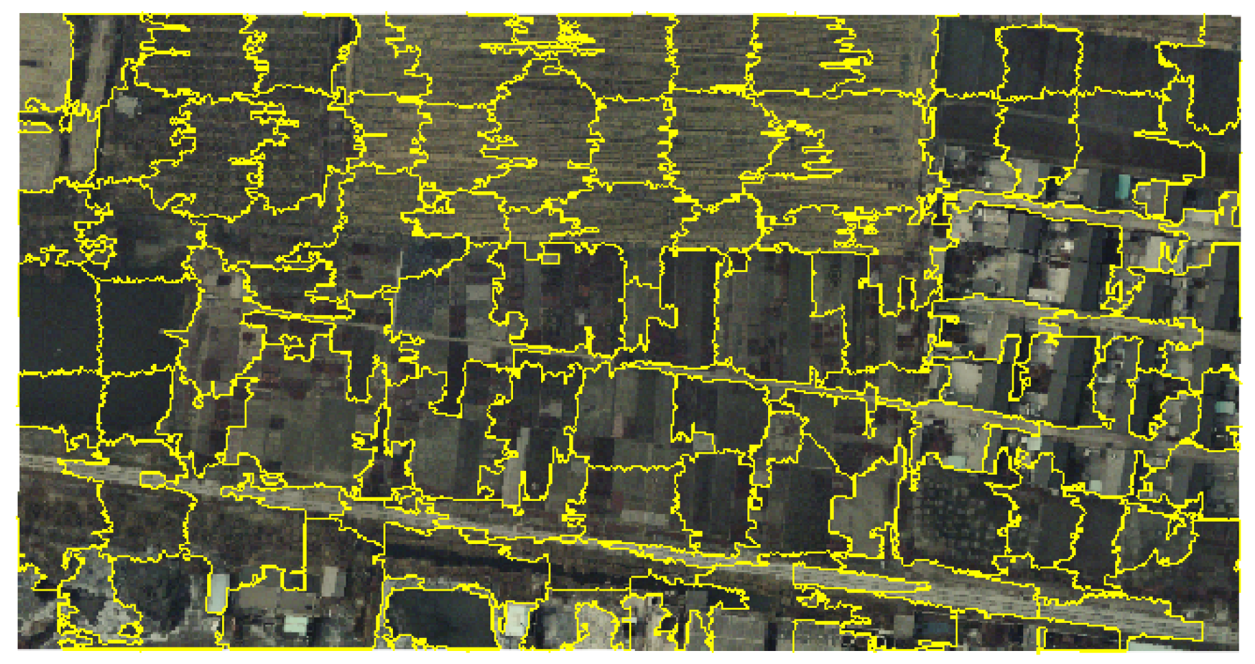Therefore, the high storage and calculation burden means that these methods can only handle small-scale HSI datasets, and they become much slower as the number n of pixels increases. To solve the problem, large-scale HSI clustering has become the key study direction, which can be roughly divided into superpixel-based methods and anchor-based methods. Superpixel-based methods use classic superpixel segmentation models like entropy rate superpixel (ERS) [18] or simple linear iterative clustering (SLIC) [19] to group similar pixels located in local neighborhoods. Pixels in the same group are generally linearly weighted as a representative pixel termed a superpixel. These superpixels are built as a symmetrical superpixel–superpixel graph to achieve clustering. Therefore, the superpixel-based method drops memory complexity to $\mathcal{O}(M^2)$ and computational complexity to $\mathcal{O}(M^3)$, where M is the number of superpixels. As $M\ll n$, it can be extended to large-scale HSI datasets. For this line, some representative works have been proposed. SGLSC [20] proposed a superpixel-level graph-learning method from both global and local aspects. The global graph is built in a self-expressed way, while the local graph is built by using the Manhattan distance to retain the nearest four superpixels. After fusing global and local graphs, spectral clustering is used to obtain the final results. More recently, EGFSC [21] simultaneously learned a superpixel-level graph and spectral-level graph for fusion. As EGFSC is a multistage model free of iterations, it is much faster than SGLSC. However, superpixel-based models have an internal limitation, i.e., they regard all the pixels in one superpixel as the same cluster. Therefore, these models cannot obtain high-quality pixel-level clustering results, and their performance is highly sensitive to the number of superpixels.

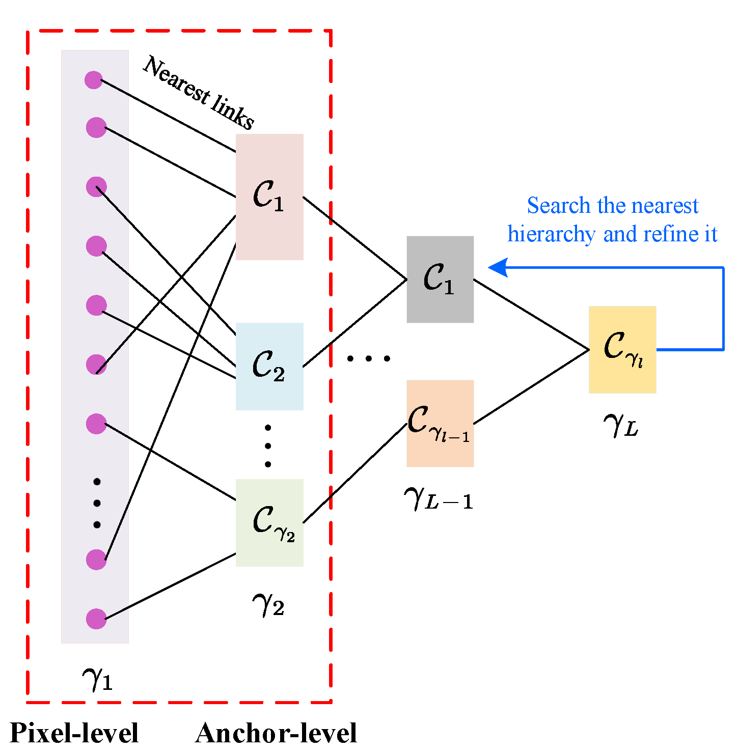
The anchor-based method is more popular for large-scale HSI clustering, which selects m representative anchors ($m\ll n$) to learn a pixel–anchor graph for clustering, and, thus, both memory and computational complexity are dropped as a linear relation to n. Some works [22,23] have used random sampling or K-means to generate anchors for pixel–anchor graph learning and then partition the clusters by conducting singular value decomposition (SVD) and extra discretization operations. To generate more reasonable anchors, a recent model, SAGC [24], used ERS to obtain superpixels and regarded the center of each superpixel as an anchor. By this way, the selected anchors reflect the spatial context, unveiling exact pixel–anchor relations. However, the multistage process and the instability of postprocessing still limit the clustering performance. More efforts have been spent to design a one-step paradigm. For example, SGCNR [25] proposed a non-negative and orthogonal relaxation method to directly obtain the cluster indicator from low-dimensional embeddings. GNMF [26] proposed a unified framework that conducts non-negative matrix factorization to yield the soft cluster indicator. SSAFC [27] proposed a joint learning framework of self-supervised spectral clustering and fuzzy clustering to directly generate the soft cluster indicator. By learning an anchor–anchor graph to provide cluster results, SAPC [28] achieves large-scale HSI clustering via label propagation. Moreover, a structured bipartite-graph-based HSI clustering model termed BGPC [29] is proposed, which conducts low-rank constraint to bipartite graphs, directly providing cluster results via connectivity. Although many efforts have been made, current works confront two problems: First, performing SVD on an $n\times m$ pixel–anchor graph leads to $\mathcal{O}(m^{2}n+m^3)$ complexity, which is still a little high. Second, many current works are based on the graph learning mode of CAN [30]. However, CAN ignored the symmetry condition of graph during the process of affinity estimation, which always generates a suboptimal graph with poor clustering results. Moreover, although some doubly stochastic graph learning methods (like DSN [31]) have been proposed to solve the problem, they rely on predefined graph inputs due to the difficulty of optimization design.

To address the issues, this paper introduces a large-scale hyperspectral image projected clustering model (abbreviated as HPCDL) via doubly stochastic graph learning. The main contributions of this paper are as follows:

• We introduce HPCDL (Code has been published at https://github.com/NianWang-HJJGCDX/HPCDL.git) (accessed on 18 February 2025), a unified framework that learns a projected feature space to simultaneously build a pixel–anchor graph and an anchor–anchor graph. The doubly stochastic constraints (symmetric, non-negative, row sum being 1) are applied to the anchor–anchor graph, combining affinity estimation and graph symmetry into one step, which ultimately produces a better graph with strict probabilistic affinity. The learned anchor–anchor graph directly derives anchor cluster indicators via its connectivity and propagates labels to pixel-level clusters through nearest-neighbor relationships in the pixel–anchor graph.
• We analyze the relationship between the proposed HPCDL and existing hierarchical clustering models from a theoretical perspective while also providing in-depth insights.
• We design an effective optimization scheme. Specifically, we first deduce a key equivalence relation and propose a novel method for optimizing the subproblem with doubly stochastic constraints. Unlike the widely used von Neumann successive projection (VNSP) lemma, our method does not require decomposition of the doubly stochastic constraints for alternating projections. Instead, it optimizes all constraints simultaneously, thereby guaranteeing convergence to a globally optimal solution.
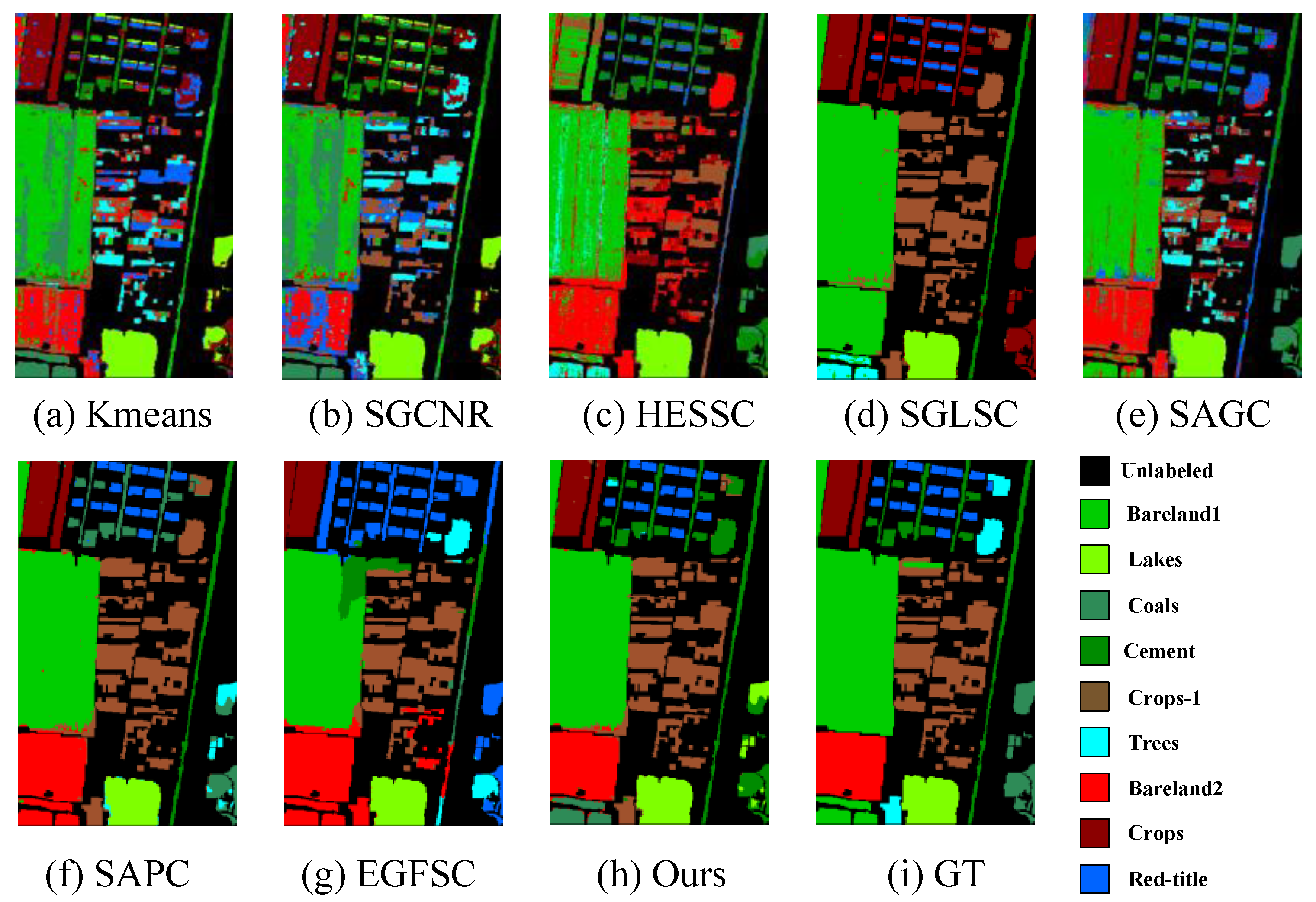
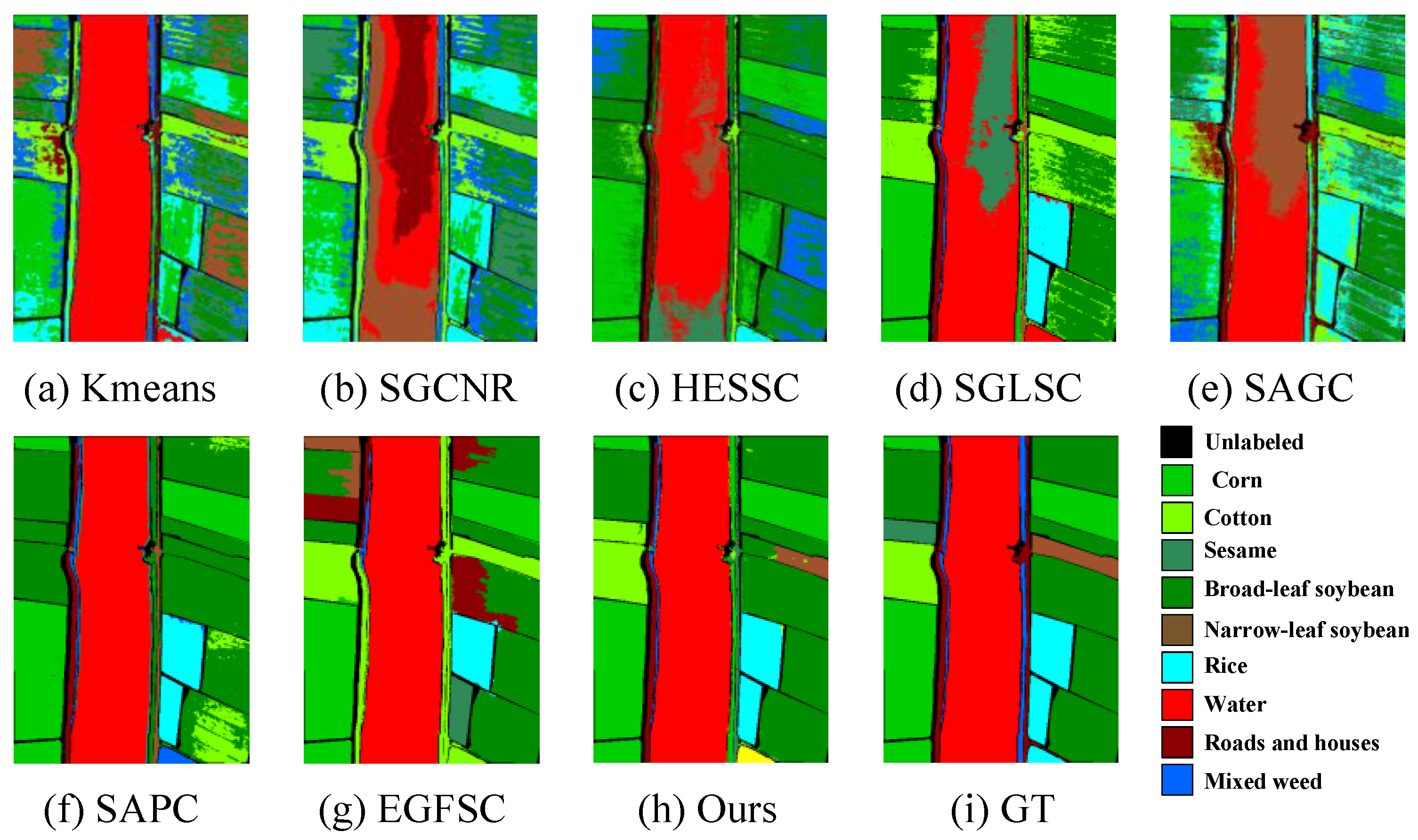
• The experiments on three widely used HSI datasets demonstrate that our method achieves state-of-the-art (SOTA) clustering performance while maintaining low computational costs, making it easily extensible to large-scale datasets.

Organization: Section 2 introduces related works. Section 3 illustrates the proposed HPCDL and then designs an effective optimization scheme. Section 4 conducts experiments to verify the merits of our proposed model. Section 5 discusses the motivation, parameters, and limitations. Section 6 concludes the paper with future research directions.

2. Related Work

2.1. Clustering with Adaptive Neighbor (CAN)

CAN [30] is a classical graph learning method that constructs a graph with probabilistic affinities, where the neighborhood relationships of each sample are adaptively determined. Formally, the model of CAN is defined as

$$\begin{array}{cc}\hfill & \underset{\mathit{W}}{min}\sum _{i,j=1}^n\left({∥{\mathbf{x}}_i-{\mathbf{x}}_j∥}_2^2{w}_{ij}+\Gamma w_{ij}^2\right)\hfill \\ & s.t.{\mathbf{1}}^T{\mathit{w}}_i=1,w_{ij}\ge 0,\hfill \end{array}$$

(1)

where $\mathit{W}$ denotes the affinity matrix of the graph. The term ${∥{\mathbf{x}}_i-{\mathbf{x}}_j∥}_2^2{w}_{ij}$ decides the affinities, which implies that any pixel ${\mathbf{x}}_j$ can be a neighbor of the $i\text{-}\mathrm{th}$ pixel ${\mathbf{x}}_i$ with probabilistic affinity $w_{ij}$. This follows the assumption that pixels with smaller Euclidean distance ${∥{\mathbf{x}}_i-{\mathbf{x}}_j∥}_2^2$ have higher connection probability $w_{ij}$. The second term $w_{ij}^2$ with a hyperparameter $\Gamma$ is used to avoid trivial solution, i.e, only the nearest pixel becomes the neighbor with probability being 1. ${\mathit{w}}_i$ denotes the i-th row of $\mathit{W}$, and $\mathbf{1}$ is a column vector with all the entries being 1. Therefore, ${\mathbf{1}}^T{\mathit{w}}_i=1$ is the row sum constraint and $w_{ij}\ge 0$ is the non-negative constraint, which bind all affinities to [0–1]. Let $d_{ij}^x={∥{\mathbf{x}}_i-{\mathbf{x}}_j∥}_2^2$. To avoid parameter tuning, [30] we set $\Gamma$ as

$$\Gamma ={\displaystyle \frac{1}{n}}{\sum }_{i=1}^n({\displaystyle \frac{c}{2}}{d}_{i,c+1}^x-{\displaystyle \frac{1}{2}}{\sum }_{j=1}^c{d}_{ij}^x),$$

(2)

where c denotes the number of neighbors. Consequently, a closed-form solution for $\mathit{W}$ can be derived as

$$w_{ij}={\displaystyle \frac{d_{i,c+1}^x-d_{ij}^x}{k{d}_{i,c+1}^x-{\sum }_{j=1}^c{d}_{ij}^x}}.$$

(3)

Furthermore, [30] proposed to use a rank constraint $rank({\mathit{L}}_{\mathit{W}})=n-k$ to Problem (1), where n denotes the number of pixels and k denotes the number of clusters. Therefore, we obtain

$$\begin{array}{cc}\hfill \underset{\mathit{W}}{min}& \sum _{i,j=1}^n\left({∥{\mathbf{x}}_i-{\mathbf{x}}_j∥}_2^2{w}_{ij}+\Gamma w_{ij}^2\right)\hfill \\ \hfill s.t.& {\mathbf{1}}^T{\mathit{w}}_i=1,w_{ij}\ge 0,rank({\mathit{L}}_{\mathit{W}})=n-k,\hfill \end{array}$$

(4)

where $rank({\mathit{L}}_{\mathit{W}})=n-k$ makes the learned $\mathit{W}$ structured, directly providing cluster indicators via connectivity. Like Problem (1), a similar optimization scheme can be used for Problem (4). Although Problem (4) succeeds in avoiding the postprocessor of discretization, it still requires manmade symmetry $\mathit{W}={\displaystyle \frac{\mathit{W}+{\mathit{W}}^T}{2}}$ as the symmetry condition of $\mathit{W}$ is ignored during affinity estimation. Such a separate process changes the affinities and always generates a suboptimal graph with fluctuating degrees.

2.2. Doubly Stochastic Graph Learning

A doubly stochastic graph is characterized as the affinity matrix $\mathit{W}$ to be ${\mathit{w}}_i={\mathit{w}}^i,{\mathbf{1}}^T{\mathit{w}}_i=1,w_{ij}\ge 0$ for all i, where ${\mathit{w}}_i={\mathit{w}}^i$ is the symmetry condition, meaning that the ith row ${\mathit{w}}_i$ and column ${\mathit{w}}^i$ of $\mathit{W}$ are equal. As recent works have learned a probabilistic graph with constraints ${\mathbf{1}}^T{\mathit{w}}_i=1,w_{ij}\ge 0$, it in essence combines the graph symmetry and affinity estimation into one step. Doubly stochastic graph learning has been studied through a long period. An early work DSN [31] proposed a doubly stochastic approximation problem as

$$\underset{\mathit{W}}{min}{\parallel \mathit{W}-\mathit{S}\parallel }_F^2,s.t.{\mathit{w}}_i={\mathit{w}}^i,{\mathbf{1}}^T{\mathit{w}}_i=1,w_{ij}\ge 0,$$

(5)

where $\mathit{S}$ is the affinity matrix of the input graph, $\mathit{W}$ is the learned doubly stochastic matrix, and ${\parallel ·\parallel }_F$ denotes the Frobenius norm.

The optimization of Problem (1) is designed by using VNSP lemma, which separates the doubly stochastic constraints and obtains two subproblems as

$$\underset{\mathit{W}}{min}{\Vert \mathit{W}-\mathit{S}\Vert }_F^2\mathrm{s}.\mathrm{t}.{\mathit{w}}_i={\mathit{w}}^i,{\mathbf{1}}^T{\mathit{w}}_i=1,$$

(6)

$$\underset{\mathit{W}}{min}{\Vert \mathit{W}-\mathit{S}\Vert }_F^2\mathrm{s}.\mathrm{t}.{\mathit{w}}_{ij}\ge 0.$$

(7)

The solutions of Problems (6) and (7) are, respectively,

$${\mathit{W}}_1=\mathit{S}+({\displaystyle \frac{1}{n}}\mathit{I}+{\displaystyle \frac{{\mathbf{1}}^{\top }\mathit{S}\mathbf{1}}{n^2}}\mathit{I}-{\displaystyle \frac{1}{n}}\mathit{S})\mathbf{1}{\mathbf{1}}^{\top }-{\displaystyle \frac{1}{n}}\mathbf{1}{\mathbf{1}}^{\top }\mathit{S},$$

(8)

$${\mathit{W}}_2={\mathit{S}}_{+},$$

(9)

where ${\mathit{S}}_{+}$ means $s_{ij}=max(s_{ij},0)$.

For each iteration, we first solve Problem (6) to obtain ${\mathit{W}}_1$, and substitute $\mathit{S}$ in Problem (7) with ${\mathit{W}}_1$. Next, we solve Problem (7) and use its solution ${\mathit{W}}_2$ to replace $\mathit{S}$ in Problem (6). The above process repeats until $\mathit{W}$ converges under the constraints of both Problems (6) and (7), at which point $\mathit{W}$ becomes a doubly stochastic matrix. Such graphs have been widely verified to clarify data structure by maintaining must-links while alleviating cannot-links (see Figure 1) [32,33,34]. Consequently, many works learned a doubly stochastic graph to improve clustering [35,36,37,38,39,40,41,42]. However, all of them followed the paradigm of DSN, which involves a doubly stochastic graph approximation problem with the VNSP-based optimization. Directly building a doubly stochastic graph from a data matrix is still an open area of investigation.

Figure 1. An example to explain the merit of doubly stochastic graph learning. (a) An ideal affinity matrix with 4 blocks, where the connections within the main diagonal are “must-links” that provide necessary connectivity, while the connections not located in the main diagonal are “cannot-links”, which denote the false similarities between different clusters. (b) A perturbed affinity matrix by adding noise to (a). (c) Doubly stochastic approximation of (b).

3. Materials and Methods

3.1. Model Definition

Despite significant progress, current graph-based HSI clustering approaches still face three critical challenges: (1) Spectral–spatial signature redundancy: The high-dimensional spectral features coupled with spatial correlations often lead to mixed and redundant representations, compromising feature discriminability. (2) Computational complexity limitations: While anchor-based methods have achieved linear complexity for large-scale HSI clustering, the subsequent cluster assignment through matrix decomposition or structured graph learning still incurs substantial computational overhead. (3) Graph construction suboptimality: Most approaches suffer from performance degradation due to the disjoint optimization of affinity estimation and graph symmetry. To solve the problems simultaneously, inspired by [28], we propose a unified framework termed HPCDL as follows:

$$\begin{array}{cc}\hfill & \underset{\mathit{P},\mathit{Z},\mathit{A},\mathit{W}}{min}\sum _{i=1}^n\sum _{j=1}^m{∥{\mathit{P}}^T{\mathbf{x}}_i-{\mathit{P}}^T{\mathit{a}}_j∥}_2^2{z}_{ij}+\gamma z_{ij}^2\hfill \\ \hfill & +\alpha (\sum _{i,j=1}^m({∥{\mathit{P}}^T{\mathit{a}}_i-{\mathit{P}}^T{\mathit{a}}_j∥}_2^2{w}_{ij}+\beta w_{ij}^2))\hfill \\ \hfill s.t.& {\mathit{P}}^T\mathit{X}{\mathit{X}}^T\mathit{P}=\mathit{I};{\mathbf{1}}^T{\mathit{z}}^i=1,{\mathit{z}}_i>0,\hfill \\ \hfill & {\mathit{w}}_i={\mathit{w}}^i,{\mathbf{1}}^T{\mathit{w}}^i=1,w_{ij}>0,rank({\mathit{L}}_{\mathit{W}})=m-k,\hfill \end{array}$$

(10)

where $\mathit{P}$ is the projected matrix and $\mathit{A}$ is the anchor matrix. Problem (10) simultaneously learns a pixel–anchor graph $\mathit{Z}$ and an anchor–anchor graph $\mathit{W}$ in a projected space based on the adaptive neighbor theory. A hyperparameter $\alpha$ is used to balance the importance of these two kinds of graphs. Moreover, $\gamma$ and $\beta$ are two hyperparameters used for the building of $\mathit{Z}$ and $\mathit{W}$, respectively, which can be set by Equation (2) to avoid parameter tuning according to the theory of CAN [30]. Therefore, only hyperparameter $\alpha$ needs to be tuned, which has an important influence for the performance of our model. As the learned pixel–anchor graph $\mathit{Z}$ does not provide clustering results, we only use ${\mathbf{1}}^T{\mathit{z}}^i=1,{\mathit{z}}_i>0$ to obtain probabilistic affinities. Moreover, the rank constraint $rank({\mathit{L}}_{\mathit{W}})=m-k$ enforces the learned affinity matrix $\mathit{W}$ to exhibit an ideal block-diagonal structure, where connected components correspond to distinct clusters. Therefore, the symmetry of $\mathit{W}$ is necessary, and we directly learn a symmetrical probabilistic graph with doubly stochastic constraints ${\mathit{w}}_i={\mathit{w}}^i,{\mathbf{1}}^T{\mathit{w}}^i=1,w_{ij}>0$. We detail the internal mechanism and merits of Problem (10) as follows:

(1) Effective spatial–spectral feature extraction. The constraint ${\mathit{P}}^T\mathit{X}{\mathit{X}}^T\mathit{P}=\mathit{I}$ reduces original d spectral bands to r orthogonal ones, eliminating redundancy and enhancing spectral feature learning. Inspired by [24], we use the ERS method to obtain local segmentations and initialize anchors as ${\mathit{a}}_i={\displaystyle \frac{1}{j}}{\sum }_j{\mathbf{x}}_j$, where i denotes the index of segmentation (see Figure 2) and j denotes the index of pixels within current segmentation. This approach ensures that the anchors effectively encode spatial information. During optimization, the projected matrix $\mathit{P}$ and anchor matrix $\mathit{A}$ are collaboratively updated to refine both spectral band selection and anchor placement, enabling effective spatial–spectral feature extraction.

Figure 2. The segmentation results from using ERS on the Xuzhou dataset. The yellow line marks the partition boundaries.

(2) Low calculation burden. Instead of using Eigen decomposition to an $n\times n$ pixel–pixel graph or an $n\times m$ pixel–anchor graph, we achieve cluster assignment on an $m\times m$ anchor–anchor graph, reducing the calculation complexity to $\mathcal{O}(m^3)$, independent of the number of pixels n. Moreover, we use the strategy in [43] to adaptively decide the number of anchors m, which stably controls m to a small but reasonable value in [100–200] across datasets of varying scales. For HSIs with hundreds of thousands of pixels, such a compact anchor set dramatically accelerates the processing speed of our HPCDL framework.

(3) Doubly stochastic graph learning. Problem (10) is a unified framework used to cooperatively optimize the projected matrix $\mathit{P}$, anchor matrix $\mathit{A}$, pixel–anchor graph $\mathit{Z}$, and anchor–anchor graph $\mathit{W}$. While exact cluster assignment on a reduced graph $\mathit{W}$ remains challenging, our approach learns a doubly stochastic anchor–anchor graph that simultaneously addresses both affinity estimation and graph symmetry. This formulation explicitly enhances the block-diagonal structure of $\mathit{W}$, thereby improving clustering accuracy. By searching for the connectivity of $\mathit{W}$, we obtain the anchor-level clusters. Subsequently, we can directly obtain the pixel-level clusters by the nearest pixel–anchor relationships encoded in $\mathit{Z}$.

For convenience, we introduce $\mathit{U}={\mathit{P}}^T\mathit{A}$ and obtain the final target function of our HPDCL as

$$\begin{array}{cc}\hfill & \underset{\mathit{P},\mathit{Z},\mathit{U},\mathit{W}}{min}\sum _{i=1}^n\sum _{j=1}^m{∥{\mathit{P}}^T{\mathbf{x}}_i-{\mathit{u}}_j∥}_2^2{z}_{ij}+\gamma z_{ij}^2\hfill \\ \hfill & +\alpha (\sum _{i,j=1}^m({∥{\mathit{u}}_i-{\mathit{u}}_j∥}_2^2{w}_{ij}+\beta w_{ij}^2))\hfill \\ \hfill s.t.& {\mathit{P}}^T\mathit{X}{\mathit{X}}^T\mathit{P}=\mathit{I};{\mathbf{1}}^T{\mathit{z}}^i=1,{\mathit{z}}_i>0,\hfill \\ \hfill & {\mathit{w}}_i={\mathit{w}}^i,{\mathbf{1}}^T{\mathit{w}}^i=1,w_{ij}>0,rank({\mathit{L}}_{\mathit{W}})=m-k.\hfill \end{array}$$

(11)

From a macro-level perspective, our proposed HPDCL is related to recent hierarchical clustering models, particularly the FINCH [44]. As shown in Figure 3, FINCH builds the cluster hierarchy $\mathit{{\rm Y}}=\left\{{\gamma }_1,{\gamma }_2,\cdots {\gamma }_L\right\}$ by constantly merging the nearest clusters. For each partition ${\gamma }_l=\left\{{\mathcal{C}}_1,{\mathcal{C}}_2,\cdots {\mathcal{C}}_{{\gamma }_l}\right\}$, it is a valid cluster assignment only when the condition ${\mathcal{C}}_{{\gamma }_l}>{\mathcal{C}}_{{\gamma }_{l+1}}$ is always satisfied. This means that the number of clusters is gradually reduced until it converges (in some cases, all the pixels are converged to one cluster). Therefore, hierarchical clustering models are fundamentally unconstrained clustering methods that do not require predefined cluster numbers. If a specific cluster number k is required, hierarchical clustering models must first identify the cluster hierarchy ${\gamma }_l$ that is closest to but exceeds k. Subsequently, a refinement strategy iteratively merges the most similar cluster pairs until ${\gamma }_l=k$ is achieved during hierarchy reorganization. In contrast, our proposed HPDCL operates as a two-hierarchy framework with the pixel-level and anchor-level hierarchies (illustrated in the red dotted box). Specifically, by imposing a rank constraint on the anchor–anchor graph, our HPCDL framework directly enforces the formation of exactly k anchor-level clusters during the hierarchy construction phase. Consequently, pixel-level clusters are simultaneously obtained through nearest-neighbor propagation based on the pixel–anchor associations encoded in $\mathit{Z}$, eliminating the need for additional hierarchy search or iterative refinement procedures.

Figure 3. An illustration to show the relation of our proposed HPDCL and recent hierarchical clustering models.

3.2. Optimization

As Problem (11) contains four variables ($\mathit{P}$, $\mathit{Z}$, $\mathit{U}$, and $\mathit{W}$), we propose an effective alternating optimization approach to iteratively update each variable until convergence.

3.2.1. Update $\mathit{P}$ with Others Fixed

Problem (11) becomes

$$\begin{array}{cc}\hfill & \underset{\mathit{P}}{min}\sum _{i=1}^n\sum _{j=1}^m{∥{\mathit{P}}^T{\mathbf{x}}_i-{\mathit{u}}_j∥}_2^2{z}_{ij}\hfill \\ \hfill & s.t.{\mathit{P}}^T\mathit{X}{\mathit{X}}^T\mathit{P}=\mathit{I}.\hfill \end{array}$$

(12)

Considering $\mathit{U}={\mathit{P}}^T\mathit{A}$, we have

$$\begin{array}{cc}\hfill & \sum _{i=1}^n\sum _{j=1}^m{∥{\mathit{P}}^T{\mathbf{x}}_i-{\mathit{P}}^T{\mathit{a}}_j∥}_2^2{z}_{ij}\hfill \\ \hfill & =2tr(\left[{\mathit{P}}^T\mathit{X}{\mathit{P}}^T\mathit{A}\right]\hfill \\ \hfill & \left.(\left[\begin{array}{cc}{\mathit{I}}_n& \mathbf{0}\\ \mathbf{0}& {\mathit{D}}_m\end{array}\right]-\left[\begin{array}{cc}\mathbf{0}& \mathit{Z}\\ {\mathit{Z}}^T& \mathbf{0}\end{array}\right]\right)\left[\begin{array}{c}{\mathit{X}}^T\mathit{P}\hfill \\ {\mathit{A}}^T\mathit{P}\hfill \end{array}\right])\hfill \\ \hfill =& 2tr\left({\mathit{P}}^T\left(\mathit{X}{\mathit{X}}^T-2\mathit{X}\mathit{Z}{\mathit{A}}^T+\mathit{A}{\mathit{D}}_m{\mathit{A}}^T\right)\mathit{P}\right).\hfill \end{array}$$

(13)

Let $\Phi =\mathit{X}{\mathit{X}}^T-2\mathit{X}\mathit{Z}{\mathit{A}}^T+\mathit{A}{\mathit{D}}_m{\mathit{A}}^T$. Problem (13) is equal to

$$\underset{{\mathit{P}}^T\mathit{X}{\mathit{X}}^T\mathit{P}=\mathit{I}}{min}Tr\left({\mathit{P}}^T\Phi \mathit{P}\right).$$

(14)

According to the generalized Rayleigh quotient, Problem (14) is equal to an eigen decomposition problem of inv($\mathit{X}{\mathit{X}}^T$)$\Phi$, where inv(·) denotes the matrix inversion operation. Therefore, the optimal solution is constructed by the eigenvectors corresponding to the r smallest eigenvalues, where r is the number of reduced spectral dimensions.

3.2.2. Update $\mathit{Z}$ with Others Fixed

Problem (11) becomes

$$\begin{array}{cc}\hfill & \underset{\mathit{Z}}{min}\sum _{i=1}^n\sum _{j=1}^m{∥{\mathit{P}}^T{\mathbf{x}}_i-{\mathit{P}}^T{\mathit{a}}_j∥}_2^2{z}_{ij}+\gamma z_{ij}^2\hfill \\ \hfill & s.t.{\mathbf{1}}^T{\mathit{z}}^i=1,{\mathit{z}}_i>0.\hfill \end{array}$$

(15)

Problem (15) is similar to Problem (1). If we set $d_{ij}^x=\parallel {{\mathit{P}}^T{\mathbf{x}}_i-{\mathit{P}}^T{\mathit{a}}_j\parallel }_2^2$, the closed-form solution of $\mathit{Z}$ can be obtained by Equation (3).

3.2.3. Update $\mathit{W}$ with Others Fixed

Problem (11) becomes

$$\begin{array}{cc}\hfill & \underset{\mathit{W}}{min}\sum _{i,j=1}^m({∥{\mathit{u}}_i-{\mathit{u}}_j∥}_2^2{w}_{ij}+\beta w_{ij}^2)\hfill \\ \hfill & s.t.{\mathit{w}}_i={\mathit{w}}^i,{\mathbf{1}}^T{\mathit{w}}^i=1,w_{ij}>0,\hfill \\ \hfill & rank({\mathit{L}}_{\mathit{W}})=n-k,\hfill \end{array}$$

(16)

which contains both the doubly stochastic constraint and rank constraint about variable $\mathit{W}$. As the rank constraint $rank({\mathit{L}}_{\mathit{W}})=n-k$ is not easy to solve, we introduce Theorem 1.

Theorem 1.

Let ${\sigma }_i({\mathit{L}}_{\mathit{W}})$ be the $i\text{-}\mathrm{th}$ smallest eigenvalue of ${\mathit{L}}_{\mathit{W}}$. We know that $\forall i\in 1,2,\cdots ,n,{\sigma }_i({\mathit{L}}_{\mathit{W}})\ge 0$ due to the semi-definite property of Laplace matrix ${\mathit{L}}_{\mathit{W}}$. Therefore, minimizing ${\sum }_{i=1}^k{\sigma }_i\left({\mathit{L}}_{\mathit{W}}\right)$ will drop the smallest k eigenvalues to be zero, and, thus, the constraint $rank({\mathit{L}}_{\mathit{W}})=n-k$ is satisfied spontaneously.

By using Theorem 1, if $\eta$ is large enough, we obtain an equivalent transformation of Problem (16) as

$$\begin{array}{cc}\hfill \underset{\mathit{W}}{min}& \sum _{i,j=1}^m\left({∥{\mathit{u}}_i-{\mathit{u}}_j∥}_2^2{w}_{ij}+\beta w_{ij}^2\right)+2\eta \sum _{i=1}^k{\sigma }_i({\mathit{L}}_{\mathit{W}})\hfill \\ \hfill s.t.& {\mathit{w}}_i={\mathit{w}}^i,{\mathbf{1}}^T{\mathit{w}}^i=1,w_{ij}>0.\hfill \end{array}$$

(17)

In practical use, following the recommendation of [30], we set $\eta =\beta$ to avoid parameter tuning. Moreover, according to Ky Fan’s theorem [45], we know that

$$\sum _{i=1}^k{\sigma }_i({\mathit{L}}_{\mathit{W}})=\underset{{\mathit{F}}^T\mathit{F}=\mathit{I}}{min}Tr({\mathit{F}}^T{\mathit{L}}_{\mathit{W}}\mathit{F}).$$

(18)

Denote a vector ${\mathit{d}}_i\in {\mathbb{R}}^{n\times 1}$ whose j-th element is $d_{ij}={∥{\mathit{u}}_i-{\mathit{u}}_j∥}_2^2$. We obtain the matrix form of Problem (17) as

$$\begin{array}{cc}\hfill \underset{\mathit{W},\mathit{F}}{min}& Tr({\mathit{D}}^T\mathit{W})+\beta {∥\mathit{W}∥}_F^2+2\eta Tr({\mathit{F}}^T{\mathit{L}}_{\mathit{W}}\mathit{F})\hfill \\ \hfill s.t.& \mathit{W}={\mathit{W}}^T,\mathit{W}\mathbf{1}=\mathbf{1},\mathit{W}\ge \mathbf{0},{\mathit{F}}^{\mathbf{T}}\mathit{F}=\mathit{I},\hfill \end{array}$$

(19)

where $\mathit{D}\in {\mathbb{R}}^{n\times n}$ is a distance matrix consisting of the vectors ${\mathit{d}}_i$.

As Problem (19) contains two variables, $\mathit{W}$ and $\mathit{F}$, an alternative optimization approach should be used.

(1) Update $\mathit{W}$ when $\mathit{F}$ is fixed. Problem (19) becomes

$$\begin{array}{cc}\hfill \underset{\mathit{W}}{min}& Tr({\mathit{D}}^T\mathit{W})+\beta {∥\mathit{W}∥}_F^2+2\eta Tr({\mathit{F}}^T{\mathit{L}}_{\mathit{W}}\mathit{F})\hfill \\ \hfill s.t.& \mathit{W}={\mathit{W}}^T,\mathit{W}\mathbf{1}=\mathbf{1},\mathit{W}\ge \mathbf{0}.\hfill \end{array}$$

(20)

This problem involves doubly stochastic constraints, which are challenging to solve due to the presence of symmetry conditions. Previous methods, such as those based on VNSP lemma, struggle to optimize this problem effectively because of the polynomial form with respect to $\mathit{W}$. To address this issue, we propose a novel approach. Firstly, by using augmenting Lagrange method ALM [46], we obtain

$$\begin{array}{cc}\hfill \underset{\mathit{W}}{min}& Tr({\mathit{D}}^T\mathit{W})+\beta {∥\mathit{W}∥}_F^2+2\eta Tr({\mathit{F}}^T{\mathit{L}}_{\mathit{W}}\mathit{F})\hfill \\ \hfill & +{\displaystyle \frac{\mu }{2}}{\parallel \mathit{W}-{\mathit{W}}^T+{\displaystyle \frac{1}{\mu }}\Lambda \parallel }_F^2\hfill \\ \hfill s.t.& \mathit{W}\mathbf{1}=\mathbf{1},\mathit{W}\ge \mathbf{0},\hfill \end{array}$$

(21)

where $\Lambda \in {\mathbb{R}}^{n\times n}$ is the Lagrange multiplier and $\mu$ is a hyperparameter of the ALM method, which is named penalty factor and should be set as a positive constant. Problem (21) embeds the symmetric condition of $\mathit{W}$ into the objective function. During the iterations, $\mu$ is magnified by the expansion coefficient $\rho$ (another hyperparameter of ALM), which speeds up to meet the symmetry condition $\mathit{W}-{\mathit{W}}^T=0$. Therefore, owing to the convex property, Problem (21) optimizes all doubly stochastic constraints simultaneously to the globally optimal solution. The remaining challenge lies in efficiently solving Problem (21), which we address by using Theorem 2.

Theorem 2.

Assume a variable $\mathit{H}$, for a problem with matrix form as

$$\begin{array}{c}\hfill \underset{\mathit{H}}{min}{\parallel \mathit{H}-{\mathit{H}}^T+\Theta \parallel }_F^2\\ \hfill s.t.\mathit{H}\mathbf{1}=\mathbf{1},\mathit{H}\ge \mathbf{0},\end{array}$$

(22)

whose objective function depends on both the variable $\mathit{H}$ and its transposed matrix ${\mathit{H}}^T$, where $\Theta$ is a matrix polynomial independent of $\mathit{H}$. As the constraints about $\mathit{H}$ are row-separable (e.g., $\mathit{H}\mathbf{1}=\mathbf{1}$, $\mathit{H}\ge 0$), it can be solved row by row, thus obtaining a set of vector-form problems as follows:

$$\begin{array}{cc}\hfill & \underset{{\mathit{h}}_{(i)}}{min}\parallel {\mathit{h}}_{(i)}-{\mathit{h}}^{(i)}+{\theta }_{(i)}{\parallel }_2^2+\parallel {\mathit{h}}^{(i)}-{\mathit{h}}_{(i)}+{\theta }^{(i)}{\parallel }_2^2\hfill \\ \hfill & s.t.\forall i,{\mathbf{1}}^T{\mathit{h}}_{(i)}=1,{\mathit{h}}_{(i)}\ge 0,\hfill \end{array}$$

(23)

where ${\mathit{h}}_{(i)}$ and ${\mathit{h}}^{(i)}$ denote the i-th row and column of $\mathit{H}$, and ${\theta }_{(i)}$ and ${\theta }^{(i)}$ denote the i-th row and column of $\Theta$. Therefore, ${\mathit{h}}_{(i)}-{\mathit{h}}^{(i)}+{\theta }_{(i)}$ and ${\mathit{h}}^{(i)}-{\mathit{h}}_{(i)}+{\theta }^{(i)}$ denote the i-th row and column of matrix $\mathit{H}-{\mathit{H}}^T+\Theta$, respectively.

An illustration is provided in Figure 4. When $i=1$, the row constraint ${\mathbf{1}}^T{\mathit{h}}_{(1)}=1,{\mathit{h}}_{(1)}\ge 0$ means that all the elements $h_{11},h_{12},\cdots ,h_{1n}$ in the first row of $\mathit{H}$ should be restricted. However, as Problem (22) contains both the variable $\mathit{H}$ and its transposed matrix ${\mathit{H}}^T$, some elements (blue in Figure 4) in the first row of $\mathit{H}$ are not restricted if we only update the first row of matrix $\mathit{H}-{\mathit{H}}^T+\Theta$ (red in Figure 4). Therefore, the terms ${\parallel {\mathit{h}}_{(i)}-{\mathit{h}}^{(i)}+{\theta }_{(i)}\parallel }_2^2$ and ${\parallel {\mathit{h}}^{(i)}-{\mathit{h}}_{(i)}+{\theta }^{(i)}\parallel }_2^2$ simultaneously restrict the i-th row and column of matrix $\mathit{H}-{\mathit{H}}^T+\Theta$ to ensure that, for any i, all the elements in constraints ${\mathbf{1}}^T{\mathit{h}}_{(i)}=1,h_{ij}\ge 0$ participate in the calculation.

Figure 4. An illustration to show the theory of Theorem 2.

By using Theorem 2, we can transform the last term of Problem (21) to the vector form. Moreover, according to the property of Laplacian matrix, we know that $2Tr({\mathit{F}}^T{\mathit{L}}_{\mathit{W}}\mathit{F})={\sum }_{i=1,j=1}^n\parallel {{\mathit{f}}_i-{\mathit{f}}_j\parallel }_2^2{w}_{ij}={\sum }_{i=1}^n{\mathit{\tau }}_{(i)}^T{\mathit{w}}_{(i)}$, where ${\mathit{\tau }}_{(i)}\in {\mathbb{R}}^{n\times 1}$ is a vector with its j-th element being ${\mathit{\tau }}_{ij}=\parallel {{\mathit{f}}_i-{\mathit{f}}_j\parallel }_2^2$. Therefore, we arrive at

$$\begin{array}{cc}\hfill \underset{{\mathit{w}}_{(i)}}{min}& {\mathit{d}}_{(i)}^T{\mathit{w}}_{(i)}+\beta {\mathit{w}}_{(i)}^2+\eta {\mathit{\tau }}_{(i)}^T{\mathit{w}}_{(i)}\hfill \\ \hfill & +{\displaystyle \frac{\mu }{2}}\parallel {\mathit{w}}_{(i)}-{\mathit{w}}^{(i)}+{\displaystyle \frac{1}{\mu }}{\mathit{\lambda }}_{(i)}{\parallel }_2^2+{\displaystyle \frac{\mu }{2}}\parallel {\mathit{w}}^{(i)}-{\mathit{w}}_{(i)}+{\displaystyle \frac{1}{\mu }}{\mathit{\lambda }}^{(i)}{\parallel }_2^2\hfill \\ \hfill s.t.& \forall i,{\mathbf{1}}^T{\mathit{w}}_{(i)}=1,w_{ij}\ge 0,\hfill \end{array}$$

(24)

where ${\mathit{w}}_{(i)}-{\mathit{w}}^{(i)}+{\displaystyle \frac{1}{\mu }}{\mathit{\lambda }}_{(i)}$ and ${\mathit{w}}^{(i)}-{\mathit{w}}_{(i)}+{\displaystyle \frac{1}{\mu }}{\mathit{\lambda }}^{(i)}$ denote the i-th row and column of matrix $\mathit{W}-{\mathit{W}}^T+{\displaystyle \frac{1}{\mu }}\Lambda$, respectively. By simple algebraic manipulation, we further obtain

$$\underset{\forall i,{\mathbf{1}}^T{\mathit{w}}_{(i)}=1,w_{ij}\ge 0}{min}\parallel {\mathit{w}}_{(i)}-{\mathit{\vartheta }}_{(i)}{\parallel }_2^2,$$

(25)

where ${\mathit{\vartheta }}_{(i)}={\displaystyle \frac{2\mu {\mathit{w}}^{(i)}-{\mathit{\lambda }}_{(i)}+{\mathit{\lambda }}^{(i)}-{\mathit{d}}_{(i)}^T-\eta {\mathit{\tau }}_{(i)}^T}{2(\beta +\mu )}}$. Problem (25) is a common problem having closed-form solution.

(2) Update $\mathit{F}$ when $\mathit{W}$ is fixed. Problem (19) becomes

$$\underset{{\mathit{F}}^T\mathit{F}=\mathit{I}}{min}Tr\left({\mathit{F}}^T{\mathit{L}}_{\mathit{W}}\mathit{F}\right).$$

(26)

Based on the Rayleigh quotient, the solution of Problem (26) is a matrix consisting of the eigenvectors corresponding to the $\mathit{k}$ smallest eigenvalues of ${\mathit{L}}_{\mathit{W}}$.

Acceleration: The optimal doubly stochastic matrix ${\mathit{W}}^{*}$ can be obtained through an alternating optimization procedure, where we iteratively update $\mathit{F}$ and $\mathit{W}$ by solving Problem (25) and Problem (26), respectively. In practice use, we can accelerate the process. Supposing that the number of connectivity for current $\mathit{W}$ is $\varpi$, after each iteration, we can decrease $\eta$ to ${\displaystyle \frac{1}{2}}\eta$ if $\varpi >k$ or increase $\eta$ to $2\eta$ if $\varpi <k$, where k is the wanted number of clusters. When $\varpi =k$ (i.e., $\mathit{W}$ is a structured matrix) and ${\mathit{D}}_{\mathit{W}}=\mathit{I}$ (i.e., $\mathit{W}$ is a doubly stochastic matrix), where ${\mathit{D}}_{\mathit{W}}$ is the degree matrix of $\mathit{W}$, we output current $\mathit{W}$ in advance. To clear the process, the optimization of Problem (19) is summarized in Algorithm 1.

Algorithm 1: Algorithm to solve Problem (19).

Input: $\mathrm{cluster}\mathrm{number}\mathit{k},\mathrm{data}\mathrm{matrix}\mathit{X};$ Output: $\mathrm{Structured}\mathrm{doubly}\mathrm{stochastic}\mathrm{matrix}\mathit{W};$ Set $1<\rho <2,$ $\mu >0;$ Initialize $\Lambda \mathrm{as}\mathrm{a}\mathrm{zero}\mathrm{matrix},\mathrm{initialize}\eta ,\mathrm{and}\mathrm{initialize}$         $\mathrm{matrix}\mathit{W}\mathrm{randomly}$;     $\mathbf{While}\mathrm{not}\mathrm{converge}\mathbf{do}$       $(1)\mathrm{Update}$$\mathit{W}\mathrm{by}\mathrm{solving}\mathrm{Problem}(25);$       $(2)\mathrm{Update}\mathit{F}\mathrm{by}\mathrm{solving}\mathrm{Problem}(26);$       $(3)\mathrm{Update}\Lambda \mathrm{by}\Lambda =\Lambda +\mu (\mathit{W}-{\mathit{W}}^T);$       $(4)\mathrm{Update}\mu \mathrm{by}\mu =\rho \mu ;$       $(5)\mathrm{Calculate}\varpi ;$       $(6)\mathrm{if}\varpi =k\mathrm{and}{\mathit{D}}_{\mathit{W}}=\mathit{I}:$            $\mathrm{Output}\mathit{W}\mathrm{in}\mathrm{advance}.$     $\mathbf{end}\mathbf{While}$

3.2.4. Update $\mathit{U}$ with Others Fixed

$$\begin{array}{c}\hfill \underset{\mathit{U}}{min}\sum _{i=1}^n\sum _{j=1}^m{∥{\mathit{P}}^T{\mathbf{x}}_i-{\mathit{u}}_j∥}_2^2{z}_{ij}+\alpha (\sum _{i,j=1}^m{∥{\mathit{u}}_i-{\mathit{u}}_j∥}_2^2{w}_{ij}).\end{array}$$

(27)

According to the deduction in Equation (13), we know that the first term is $-2Tr({\mathit{P}}^T\mathit{X}\mathit{Z}\mathit{U}+\mathit{U}{\mathit{D}}_m{\mathit{U}}^T)$ after removing the independent terms. Moreover, we know that ${∥{\mathit{u}}_i-{\mathit{u}}_j∥}_2^2{w}_{ij}=2Tr(\mathit{U}{\mathit{L}}_{\mathit{W}}{\mathit{U}}^T)$, where ${\mathit{L}}_{\mathit{W}}$ denotes the Laplace matrix of the anchor–anchor graph $\mathit{W}$. Combining with them, we transfer Problem (27) as

$$\begin{array}{c}\hfill \underset{\mathit{U}}{min}Tr(\mathit{U}(2\alpha {\mathit{L}}_{\mathit{W}}+{\mathit{D}}_m){\mathit{U}}^T-2{\mathit{P}}^T\mathit{X}\mathit{Z}\mathit{U}).\end{array}$$

(28)

By taking the derivative with respect to $\mathit{U}$ and setting it to zero, we obtain the optimal solution of Problem (28) as

$$\mathit{U}={\mathit{P}}^T\mathit{X}\mathit{Z}{({\mathit{D}}_m+2\alpha {\mathit{L}}_{\mathit{W}})}^{-1}.$$

(29)

At this point, we have completed the updates of all variables. The whole optimization process is summarized in Algorithm 2.

Algorithm 2: Algorithm to solve Problem (11).

Input: $\mathrm{data}\mathrm{matrix}\mathit{X},\mathrm{cluster}\mathrm{number}\mathit{k};$ Output: $\mathrm{Pixel}-\mathrm{level}\mathrm{clustering}\mathrm{results}$; Initialize $\mathrm{anchor}\mathrm{matrix}\mathit{A}\mathrm{and}\mathrm{pixel}--\mathrm{anchor}\mathrm{matrix}\mathit{Z};$     $\mathbf{While}\mathrm{not}\mathrm{converge}\mathbf{do}$       $(1)\mathrm{Update}$ $\mathit{P}\mathrm{by}\mathrm{solving}\mathrm{Problem}(14);$       $(2)\mathrm{Update}$ $\mathit{Z}\mathrm{by}\mathrm{solving}\mathrm{Problem}(15);$       $(3)\mathrm{Update}$ $\mathit{W}\mathrm{by}\mathrm{Algorithm}1;$       $(4)\mathrm{Update}$ $\mathit{U}\mathrm{by}\mathrm{Equation}(29);$     $\mathbf{end}\mathbf{While}$     $\mathrm{Obtain}\mathrm{anchor}-\mathrm{level}\mathrm{clusters}\mathrm{via}\mathrm{the}\mathrm{connectivity}\mathrm{of}\mathit{W}$     $\mathrm{and}\mathrm{propagate}\mathrm{it}\mathrm{to}\mathrm{pixel}-\mathrm{level}\mathrm{results}.$

3.3. Computational Complexity Analysis

In the preprocessing stage, superpixel segmentation of HSI data by using ERS requires $\mathcal{O}\left(nlog(n)\right)$ complexity, where n is the number of pixels. Notably, this is necessary for large-scale HSI clustering models that use superpixel segmentation to drop the complexity. For our model, four variables should be updated during the iterations. First, updating $\mathit{Z}$ requires $\mathcal{O}\left(nmd\right)$, where m and d denote the number of anchors and spectral signatures, respectively. Moreover, updating projected matrix $\mathit{P}$ requires $\mathcal{O}\left(d^3\right)$. To update the structured doubly stochastic matrix $\mathit{W}$, we need to impose eigen decomposition on a $m\times m$ anchor–anchor graph, which requires $\mathcal{O}\left(m^3\right)$ complexity. Finally, updating projected anchor matrix $\mathit{U}$ needs $\mathcal{O}\left(m^3\right)$ due to the matrix inversion operation. As $n\gg d$ and $n\gg m$, the overall complexity of our model is mainly caused by $\mathcal{O}\left(nmd\right)$, which is less than recent works that impose eigen decomposition on an $n\times n$ graph or an $n\times m$ graph, causing $\mathcal{O}\left(n^3+nmd\right)$ or $\mathcal{O}\left(n{m}^2+nmd\right)$ complexity in the iterations. After the iterative process, the label propagation from anchor-level to pixel-level incurs a computational complexity of $\mathcal{O}(nm)$. However, this cost becomes negligible when compared to the computational overhead of the iteration process itself. Therefore, our proposed model requires less computational complexity than recent works.

4. Experimental Results

4.1. Comparative Methods and Experimental Setting

Comparative methods include K-means [3], SGCNR [25], HESSC [11], SGLSC [20], SAGC [24], SAPC [28], and EGFSC [21]. K-means is a classic centroid-based method and HESSC is a subspace-based method. All other methods are recent graph-based models designed for large-scale HSI data. For these graph-based methods, we construct the graph using five nearest neighbors. Moreover, for SGCNR, SGLSC, SAGC, AOPL, and our proposed HPCDL, they request to initialize the anchor matrix. As aforementioned, we use the center of each superpixel as the anchor; thus, the anchor number is strictly equal to the number of superpixels. For all the methods, the hyperparameters are set to the optimal values stated in the original paper. The experiments are conducted on a Windows 10 computer with 2.3 GHz Intel Xeon Gold 5218 CPU, 128 GB RAM, MATLAB 2020b.

4.2. Data Description

Three publicly available HSI datasets are used to verify the clustering ability of our proposed method. These datasets vary in scale, allowing us to simultaneously evaluate the method’s scalability to large-scale data.

The Xuzhou dataset was published in 2014, and captures the scene of the peri-urban region in Xuzhou City, Jiangsu Province, China, having 130,000 pixels (500 × 260) and 436 spectral bands. The image was captured by an airborne hyperspectral camera and there are nine diverse categories in total. For details, see Table 1.

Table 1. Description of Xuzhou dataset.

No.	Class Name	Samples
1	Bareland1	26,396
2	Lakes	4027
3	Coals	2783
4	Crops-1	5214
5	Cement	13,184
6	Trees	2436
7	Bareland2	6990
8	Crops	4777
9	Red-title	3070
Total		68,877

The Longkou dataset was published in 2018, which is a scene of Longkou Town, Hubei Province, China. This image was captured by UAVborne system, having 220,000 pixels ($550\times 400$) and 270 bands to describe nine land-cover materials. For details, see Table 2.

Table 2. Description of Longkou dataset.

No.	Class Name	Samples
1	Corn	34,511
2	Cotton	8374
3	Sesame	3031
4	Broad-leaf soybean	63,212
5	Narrow-leaf soybean	4151
6	Rice	11,854
7	Water	67,056
8	Roads and houses	7124
9	Mixed weed	5229
Total		204,542

The Pavia Centor (PaviaC for short) dataset was published in 2003, which captures in the city of Pavia, Italy, having 783,640 pixels (1096 × 715) and 102 spectral bands. The image is captured by a reflective optics system imaging spectrometer sensor and there are nine diverse categories in total. For details, see Table 3.

Table 3. Description of PaviaC dataset.

No.	Class Name	Samples
1	Water	65,971
2	Trees	7598
3	Asphalt	3090
4	Self-blocking bricks	2685
5	Bitumen	6584
6	Tiles	9248
7	Shadows	7287
8	Meadows	42,826
9	Bare Soil	2863
Total		148,152

4.3. Metrics

We utilize user accuracy to evaluate the performance of each land-cover category. Moreover, to clearly define all the used overall metrics, we first introduce the concept of the confusion matrix. Assuming the total number of classes as k, the confusion matrix can be defined as a k-dimensional square matrix as follows:

$$\mathit{M}=\left[\begin{array}{ccccc}{m}_{11}& m_{12}& m_{13}& \cdots & m_{1k}\\ m_{21}& m_{22}& m_{23}& \cdots & m_{2k}\\ m_{31}& m_{32}& m_{33}& \cdots & m_{3k}\\ ⋮& ⋮& ⋮& \ddots & ⋮\\ m_{k1}& m_{k2}& m_{k3}& \cdots & m_{kk}\end{array}\right],$$

where $m_{ij}$ denotes the number of pixels that belong to cluster i but are assigned to cluster j. Thus, the diagonal elements $m_{ii}$ ( $i\in 1,2,\cdots ,k$) represent the number of correctly clustered pixels in the i-th land-cover category. Furthermore, the sum of all elements ${\sum }_{i,j}^k{m}_{ij}$ must equal the total number of pixels n.

Overall accuracy (OA) represents the proportion of correctly clustered pixels to the total number of pixels, which can be defined as

$$\mathrm{OA}={\displaystyle \frac{{\sum }_{i=1}^k{m}_{ii}}{n}}.$$

Kappa is another commonly used metric, which considers the influence of random factors when evaluating the accuracy of classification results. The mathematical definition is

$$Kappa={\displaystyle \frac{n{\sum }_{i=1}^k{m}_{ii}-{\sum }_{i=1}^k(m_{i,:}\times m_{:,i})}{n^2-{\sum }_{i=1}^k(m_{i,:}\times m_{:,i})}},$$

where $m_{i,:}$ and $m_{:,i}$ denote the sum of the ith row or the ith column of the confusion matrix $\mathit{M}$, respectively.

Normalized mutual information (NMI) reveals the degree of shared mutual information between a pair of clusterings. The mathematical definition is

$$NMI={\displaystyle \frac{{\displaystyle \sum _{i=1}^k}{\displaystyle \sum _{j=1}^k}{m}_{ij}log\frac{n{m}_{ij}}{m_{i,:}{m}_{:,j}}}{\sqrt{{\displaystyle \sum _{i=1}^k}{m}_{i,:}log\frac{m_{i,:}}{n}}\sqrt{{\displaystyle \sum _{j=1}^k}{m}_{:,j}log\frac{m_{:,j}}{n}}}}.$$

Purity aims to estimate the degree to which every cluster covers the pixels from one class. The mathematical definition is

$$Purity={\displaystyle \frac{1}{n}}\sum _j^k\underset{i}{max}{m}_{ij}.$$

Adjusted Rand Index (ARI) is a metric for evaluating the similarity between clustering results, which corrects for bias introduced by random label assignments to enhance comparability. The mathematical definition is

$$ARI={\displaystyle \frac{{\sum }_{i,j=1}^k{m}_{ij}^2-{\displaystyle \frac{{\sum }_{i=1}^k{m}_{i,:}^2{\sum }_{j=1}^k{m}_{:,j}^2}{n^2}}}{{\displaystyle \frac{{\sum }_{i=1}^k{m}_{i,:}^2+{\sum }_{j=1}^k{m}_{:,j}^2}{2}}-{\displaystyle \frac{{\sum }_{i=1}^k{m}_{i,:}^2{\sum }_{j=1}^k{m}_{:,j}^2}{n^2}}}}.$$

4.4. Experiments on Benchmarks

To comprehensively evaluate clustering performance and time cost across datasets of different scales, we selected Xuzhou, Longkou, and Pavia as small-, medium-, and large-scale datasets, respectively, based on their total pixel counts. We compare both of the quantitative metrics and visual maps. As the comparative methods contain both iteration-based models and non-iteration-based models, we report the average time cost per iteration for fair comparison.

(1) Results of Small-Scale Dataset Xuzhou: We first report the performance on Xuzhou, which is a small-scale dataset containing 130,000 pixels. For our method, we set r and $\alpha$ as $2d/5$ and 1 to ensure the optimal performance, where d is the total number of spectral dimensions. Table 4 reports the quantitative results. As can be seen, none of the models can ensure high accuracy for each land-cover. Our HPCDL fails to recognize Coals and Trees, which is mainly caused by the anchor strategy. As mentioned earlier, we use the mean value of all pixels within a segmentation as an anchor, which inevitably leads to information loss and complicates precise classification. More importantly, as all the pixels within a segmentation are assigned to the same cluster, a misclassified anchor can result in large-scale pixel misclassification, severely degrading accuracy (even to zero) for certain land-cover types. Nevertheless, our HPCDL obtains high metrics for OA, kappa, NMI, purity and ARI, demonstrating the excellent clustering performance. Moreover, thanks to the lower calculation complexity, our HPCDL needs lower time cost than most other methods, except for K-means. The visual maps are provided in Figure 5. As can be seen, K-means, SGCNR, HESSC, and SAGC obtain a very non-smooth clustering map, which shows that these methods cannot effectively retain the consistency of local regions. Moreover, SGLSC, SAPC, and EGFSC obtain smoother maps and show strong local capabilities in some land-covers like Bareland2 and Red-title, demonstrating their excellent classification performance for some categories. However, for certain land-covers (e.g., Cement), our proposed model performs better and well recognizes related regions, which ensures that our model achieves the best values for five overall metrics. The results show that the doubly stochastic property of anchor–anchor graphs improves clustering to some extent.

Table 4. Quantitative comparison on small-scale dataset Xuzhou. Numbers in bold denote the best results.

No.	Type	K-means	SGCNR	HESSC	SGLSC	SAGC	SAPC	EGFSC	Ours
1	Bareland1	0.5919	0.4448	0.9983	0.8975	0.8009	0.8733	0.7550	0.8788
2	Lakes	0.9650	0.9647	0.9939	0.9637	0.9434	0.9516	0.9933	0.9816
3	Coals	0.0000	0.0000	0.0000	0.0000	0.7923	0.6493	0.0000	0.0000
4	Cement	0.5084	0.5198	0.7948	0.4208	0.7236	0.4503	0.1437	0.9933
5	Crops-1	0.2855	0.4279	0.0022	0.9980	0.3108	0.9980	0.8824	0.9992
6	Trees	0.0000	0.4754	0.8761	0.0000	0.0000	0.0000	0.4823	0.0000
7	Bareland2	0.7136	0.5326	0.7194	0.0000	0.8169	0.9850	1.0000	0.9854
8	Crops	0.9525	0.9510	0.5278	0.9979	0.9860	0.9937	0.7279	0.9849
9	Red-title	0.4326	0.0007	0.2777	0.5384	0.6111	0.9225	1.0000	0.9228
OA		0.5342	0.4850	0.5803	0.7164	0.6869	0.8517	0.7408	0.8701
Kappa		0.4464	0.4042	0.4767	0.6282	0.6197	0.8135	0.6832	0.8368
NMI		0.5176	0.5268	0.5347	0.7138	0.6246	0.8251	0.6809	0.8369
Purity		0.7247	0.7267	0.6643	0.7376	0.7422	0.8806	0.7723	0.8968
ARI		0.4064	0.3962	0.4111	0.6158	0.5992	0.7884	0.6362	0.8187
Time cost		1.9759	5.5613	106.3162	43.3164	9.4736	2.4362	2.8475	2.2453

Figure 5. The visual maps for the clustering outputs on the Xuzhou dataset.

(2) Results of Medium-Scale Dataset Longkou: We then evaluated the performance on Longkou, which is a medium-scale dataset containing 220,000 pixels. For our method, we set r and $\alpha$ as $d/5$ and 100, respectively, to ensure the optimal performance. Examining the results in Table 5, our method obtains much better results for all the five metrics: OA, kappa, NMI, purity, and ARI. For the accuracy of each land-cover, our method obtains high accuracy for most of them, and for five out of nine, it obtains the best values. Moreover, our method achieves the second-lowest time cost, outperforming other graph-based methods while remaining only slightly higher than that of K-means. Figure 6 presents the visual maps. As shown, while K-means achieves accurate classification for most Water regions, it produces significant misclassification for other land-cover types. The methods SGCNR, HESSC, and SAGC exhibit patchy misclassification in Water areas along with scattered noise in other regions. In comparison, SAPC and EGFSC generate visually smoother clustering results, though they completely misclassify certain Narrow-leaf soybean and Rice areas. Our proposed model demonstrates superior performance by correctly classifying most of these challenging regions.

Table 5. Quantitative comparison on medium-scale dataset Longkou. Numbers in bold denote the best results.

No.	Type	K-means	SGCNR	HESSC	SGLSC	SAGC	SAPC	EGFSC	Ours
1	Corn	0.6433	0.5184	0.9119	0.9983	0.5947	0.9973	0.9387	0.9993
2	Cotton	0.5515	0.8360	0.1222	0.9939	0.5252	0.0000	0.9694	0.9904
3	Sesame	0.3425	0.1363	0.0000	0.0000	0.6674	0.0000	0.0000	0.0000
4	Broad-leaf soybean	0.2788	0.3546	0.7226	0.7948	0.3792	0.8713	0.7531	0.9940
5	Narrow-leaf soybean	0.0007	0.0000	0.0000	0.0022	0.0000	0.0000	0.0000	0.6018
6	Rice	0.3382	0.6435	0.0862	0.8761	0.7760	0.8827	0.6022	0.9963
7	Water	0.9978	0.3436	0.7682	0.7194	0.6065	0.9579	0.9995	0.9997
8	Roads and houses	0.3984	0.0000	0.4910	0.5278	0.9214	0.5268	0.1165	0.5284
9	Mixed weed	0.4343	0.4808	0.0522	0.2777	0.0029	0.3033	0.1320	0.2855
OA		0.5941	0.3955	0.6574	0.7669	0.5249	0.8288	0.8008	0.9400
Kappa		0.5074	0.3169	0.5545	0.7079	0.4480	0.7713	0.7442	0.9204
NMI		0.6235	0.5916	0.6148	0.7730	0.6302	0.7999	0.8085	0.9121
Purity		0.8023	0.7988	0.8157	0.8884	0.8171	0.8920	0.8882	0.9518
ARI		0.6317	0.3605	0.5125	0.6911	0.4643	0.7547	0.8220	0.9521
Time cost		3.4823	16.6532	206.4234	122.5439	74.4623	5.6463	6.9392	4.9642

Figure 6. The visual maps for the clustering outputs on the Longkou dataset.

(3) Results of Large-Scale Dataset PaviaC: We finally evaluate the performance on PaviaC, which is a large-scale dataset with 783,640 pixels. For our method, r and $\alpha$ are set as $2d/5$ and 10 to ensure optimal performance. Table 6 and Figure 7 present the quantitative results and visual clustering maps, respectively. The results demonstrate that our method achieves the highest accuracy for Water, Bitumen, and Meadows among all land-cover categories. While showing competitive performance for other land-cover types, it exhibits relatively lower accuracy only for Asphalt and Self-blocking bricks. Significantly, our method outperforms all comparative approaches across five metrics (OA, kappa, NMI, purity, and ARI), with marginal improvement over the recent SAPC method and substantial gains over other baselines, demonstrating its robust clustering capability.

Table 6. Quantitative comparison on large-scale dataset PaviaC. Numbers in bold denote the best results.

No.	Type	K-means	SGCNR	HESSC	SGLSC	SAGC	SAPC	EGFSC	Ours
1	Water	0.9936	0.9719	0.9705	0.9449	0.9942	1.0000	0.9895	1.0000
2	Trees	0.6490	0.8094	1.0000	0.4435	0.9156	0.9763	0.1640	0.9902
3	Asphalt	0.1748	0.0000	0.0000	0.0000	0.3201	0.0000	0.0243	0.0000
4	Self-blocking bricks	0.0369	0.7520	0.0000	0.1192	0.0108	0.1210	0.8104	0.2534
5	Bitumen	0.3171	0.2482	0.5556	0.0002	0.4550	0.7167	0.7075	0.8408
6	Tiles	0.8915	0.4531	0.1851	0.9976	0.6377	0.9670	0.3248	0.9524
7	Shadows	0.1772	0.5108	0.7596	0.7830	0.0008	0.7834	0.8666	0.8124
8	Meadows	0.5004	0.5357	0.9530	0.9841	0.9519	0.9979	0.6596	0.9982
9	Bare Soil	0.0010	1.0000	0.4013	0.0000	0.9511	0.8631	0.3929	0.8557
OA		0.7032	0.7265	0.8403	0.8309	0.8501	0.9334	0.7568	0.9378
Kappa		0.5917	0.6312	0.7630	0.7632	0.7845	0.9055	0.6667	0.9163
NMI		0.6906	0.7278	0.7012	0.8082	0.7762	0.9097	0.6567	0.9190
Purity		0.8314	0.8611	0.8440	0.8595	0.8624	0.9351	0.8276	0.9399
ARI		0.7653	0.7999	0.7291	0.8644	0.8693	0.9743	0.8161	0.9778
Time cost		9.2943	19.8293	489.6434	256.5431	34.4723	20.6463	22.2648	17.4592

Figure 7. The visual maps for the clustering outputs on the PaviaC dataset.

5. Discussion

5.1. Motivation Verification

This subsection verifies whether learning a doubly stochastic graph can lead to a better graph with improved connectivity and clustering performance. To achieve this, we set a Variant A that removes the symmetry condition of our HPCDL model and manually makes $\mathit{W}$ symmetrical after each iteration. Therefore, like many other graph-based models, Variant A separately conducts affinity estimation and graph symmetry. Figure 8 reports the results. As can be seen, Variant A learns a graph with fluctuating degrees, causing some “cannot-links” that influence the connectivity of the graph. Therefore, such a graph cannot provide exact anchor clusters and then obtain suboptimal pixel clustering results with lower overall accuracy (OA). By learning a doubly stochastic graph, our HPCDL combines the affinity estimation and graph symmetry into one step, generating strict probabilistic affinities with the degrees of all pixels being 1. Such a doubly stochastic graph provides clearer block-diagonal structures and more exact cluster relations. By searching for the connectivity, better clustering results are obtained.

Figure 8. The learned anchor–anchor graph on different HSI datasets. The first row and second row report the results of Variant A and HPCDL, respectively. Below each graph, the overall accuracy is shown. The third row visualizes the degrees of learned anchor–anchor graph; our HPCDL generates strict probabilistic affinities with all the degrees being 1.

We further show that our doubly stochastic graph learning method can effectively improve recent works. Two baselines, termed SAPC and EGFSC, are used. SAPC learns the graph via the adaptive neighbor theory of CAN. Therefore, after affinity estimation, a manmade symmetry operation is needed. EGFSC uses the heat kernel to build the graph and then constrains the neighbors by sorting the Euclidean distance. Our doubly stochastic graph learning method has obvious theoretical merit as it combines affinity estimation, neighbor decision, and graph symmetry into one step. To verify the effectiveness, we use our method to replace the graph learning method in SAPC and EGFSC, and then test it on the Longkou dataset. Table 7 reports the results. Our proposed method significantly improves the performance of SAPC and EGFSC as it solves the limitation of artificial intervention and multistage design. Moreover, by examining the results of SAPC and EGFSC, we observe that if the learned graph directly provides clustering results based on its connectivity (as in SAPC), the improvement achieved by our method is more significant, as it eliminates the need for K-means postprocessing. The results demonstrate that our method has the potential to enhance the performance of related works.

Table 7. The results on the Longkou dataset when using our doubly stochastic graph (DSG) learning method compared to recent graph-based clustering works.

	OA	Kappa	NMI	Purity	ARI
SAPC	0.8288	0.7713	0.7999	0.8920	0.7547
SAPC + DSG	0.8672	0.8231	0.8349	0.9212	0.7986
EGFSC	0.8008	0.7442	0.8085	0.8882	0.8220
EGFSC + DSG	0.8213	0.7634	0.8164	0.9047	0.8274

5.2. Parameter Study

First, following [30], hyperparameters $\gamma$, $\beta$, and $\eta$ are automatically determined by the number of neighbors; thus, they do not need to be tuned. Moreover, we use the ALM method to optimize Problem (20) with three more hyperparameters, $\rho$, $\mu$, and $\Lambda$. $\Lambda$ only needs to be initialized as an all-zero matrix. Penalty factor $\mu$ and expansion coefficient $\rho$ do not need to be tuned as they are suggested as $\mu =1$ and $\rho =1.1$ to ensure the stability of the ALM method [46]. Therefore, for the proposed HPCDL model, only $\alpha$ and r should be studied. $\alpha$ weighs the important of pixel–anchor and anchor–anchor graphs. r denotes the reduced spectral dimension, which avoids redundant information. We study their influence by setting $\alpha \in \{0.01,0.1,1,10,100\}$ and $r\in \{d/5,2d/5,3d/5,4d/5,d\}$, where d is the total spectral dimension. The results of overall accuracy (OA) are reported in Figure 9. As can be seen, our HPCDL obtains better results when $\alpha \in$ [1–100]. This is theoretically explainable. As the learned anchor–anchor graph directly provides cluster indicators, our model requests to underline its importance to ensure accuracy. Moreover, we notice that using both a small or large spectral dimension r drops the performance of our proposed HPCDL, which shows that a too-large r introduces some redundant and mixed spectral signatures, while a too-small r limits the richness of feature dimensions.

Figure 9. Parameter sensitivity experiment for reduced spectral dimension r and balancing hyperparameter $\alpha$.

5.3. Limitations

Our HPCDL simultaneously learns both the pixel–anchor graph and anchor–anchor graph, which is sensitive to the value of $\alpha$. Experimental results demonstrate that $\alpha$ values within the range [1–100] typically yield better performance. Moreover, it is a tractable problem to decide the specific number of reduced spectral dimension. Therefore, although we have proposed some strategies to reduce manually set hyperparameters, our proposed model still requires slight parameter tuning and is sensitive to these parameters.

6. Conclusions

This paper proposes a large-scale HSI clustering model, termed HPCDL, by a unified framework for learning a pixel–pixel graph and an anchor–anchor graph in a projected space. A novel and effective optimization method for the subproblem with doubly stochastic constraints is proposed, which can be widely used in related graph-based clustering works. Experiments on three HSI datasets showed that our method achieves SOTA clustering performance and needs lower time cost than most of the other comparatives. In the future, we will extend the current framework to deal with multitemporal data, and explore its potential adaptation to multimodal data (e.g., HSI and LiDAR) fusion-based clustering.

References

- Zhang, Z.; Cai, Y.; Gong, W.; Ghamisi, P.; Liu, X.; Gloaguen, R. Hypergraph Convolutional Subspace Clustering With Multihop Aggregation for Hyperspectral Image. IEEE J. Sel. Top. Appl. Earth Obs. Remote Sens. 2022, 15, 676–686. [Google Scholar] [CrossRef]
- Wang, N.; Yang, A.; Cui, Z.; Ding, Y.; Xue, Y.; Su, Y. Capsule Attention Network for Hyperspectral Image Classification. Remote Sens. 2024, 16, 4001. [Google Scholar] [CrossRef]
- Ranjan, S.; Nayak, D.R.; Kumar, K.S.; Dash, R.; Majhi, B. Hyperspectral image classification: A k-means clustering based approach. In Proceedings of the 2017 4th International Conference on Advanced Computing and Communication Systems (ICACCS), Coimbatore, India, 6–7 January 2017; pp. 1–7. [Google Scholar] [CrossRef]
- Yang, X.; Zhu, M.; Sun, B.; Wang, Z.; Nie, F. Fuzzy C-Multiple-Means Clustering for Hyperspectral Image. IEEE Geosci. Remote Sens. Lett. 2023, 20, 1–5. [Google Scholar] [CrossRef]
- Zhang, F.; Yan, H.; Zhao, J.; Hu, H. Euler Kernel Mapping for Hyperspectral Image Clustering via Self-Paced Learning. Remote Sens. 2024, 16, 4097. [Google Scholar] [CrossRef]
- Pei, S.; Chen, H.; Nie, F.; Wang, R.; Li, X. Centerless Clustering. IEEE Trans. Pattern Anal. Mach. Intell. 2023, 45, 167–181. [Google Scholar] [CrossRef]
- Cariou, C.; Chehdi, K.; Le Moan, S. Improved Nearest Neighbor Density-Based Clustering Techniques with Application to Hyperspectral Images. In Proceedings of the ICASSP 2020—2020 IEEE International Conference on Acoustics, Speech and Signal Processing (ICASSP), Barcelona, Spain, 4–8 May 2020; pp. 4127–4131. [Google Scholar] [CrossRef]
- Nie, F.; Liu, C.; Wang, R.; Li, X. A Novel and Effective Method to Directly Solve Spectral Clustering. IEEE Trans. Pattern Anal. Mach. Intell. 2024, 46, 10863–10875. [Google Scholar] [CrossRef]
- Zhang, H.; Zhai, H.; Zhang, L.; Li, P. Spectral–Spatial Sparse Subspace Clustering for Hyperspectral Remote Sensing Images. IEEE Trans. Geosci. Remote Sens. 2016, 54, 3672–3684. [Google Scholar] [CrossRef]
- Huang, S.; Zhang, H.; Pižurica, A. Subspace Clustering for Hyperspectral Images via Dictionary Learning with Adaptive Regularization. IEEE Trans. Geosci. Remote Sens. 2022, 60, 1–17. [Google Scholar] [CrossRef]
- Rafiezadeh Shahi, K.; Khodadadzadeh, M.; Tusa, L.; Ghamisi, P.; Tolosana-Delgado, R.; Gloaguen, R. Hierarchical sparse subspace clustering (HESSC): An automatic approach for hyperspectral image analysis. Remote Sens. 2020, 12, 2421. [Google Scholar] [CrossRef]
- Chen, J.; Liu, S.; Wang, H. Dual smooth graph convolutional clustering for large-scale hyperspectral images. IEEE J. Sel. Top. Appl. Earth Obs. Remote Sens. 2024, 17, 6825–6840. [Google Scholar] [CrossRef]
- Luo, F.; Liu, Y.; Duan, Y.; Guo, T.; Zhang, L.; Du, B. SDST: Self-supervised double-structure transformer for hyperspectral images clustering. IEEE Trans. Geosci. Remote Sens. 2024, 62, 1–14. [Google Scholar] [CrossRef]
- Yang, A.; Li, M.; Ding, Y.; Xiao, X.; He, Y. An Efficient and Lightweight Spectral-Spatial Feature Graph Contrastive Learning Framework for Hyperspectral Image Clustering. IEEE Trans. Geosci. Remote Sens. 2024. [Google Scholar] [CrossRef]
- Cai, Y.; Zhang, Z.; Cai, Z.; Liu, X.; Jiang, X.; Yan, Q. Graph convolutional subspace clustering: A robust subspace clustering framework for hyperspectral image. IEEE Trans. Geosci. Remote Sens. 2020, 59, 4191–4202. [Google Scholar] [CrossRef]
- Liu, S.; Wang, H. Graph convolutional optimal transport for hyperspectral image spectral clustering. IEEE Trans. Geosci. Remote Sens. 2022, 60, 1–13. [Google Scholar] [CrossRef]
- Cai, Y.; Zhang, Z.; Ghamisi, P.; Ding, Y.; Liu, X.; Cai, Z.; Gloaguen, R. Superpixel contracted neighborhood contrastive subspace clustering network for hyperspectral images. IEEE Trans. Geosci. Remote Sens. 2022, 60, 1–13. [Google Scholar] [CrossRef]
- Liu, M.Y.; Tuzel, O.; Ramalingam, S.; Chellappa, R. Entropy rate superpixel segmentation. In Proceedings of the CVPR 2011, Colorado Springs, CO, USA, 20–25 June 2011; pp. 2097–2104. [Google Scholar]
- Achanta, R.; Shaji, A.; Smith, K.; Lucchi, A.; Fua, P.; Süsstrunk, S. SLIC superpixels compared to state-of-the-art superpixel methods. IEEE Trans. Pattern Anal. Mach. Intell. 2012, 34, 2274–2282. [Google Scholar] [CrossRef]
- Zhao, H.; Zhou, F.; Bruzzone, L.; Guan, R.; Yang, C. Superpixel-level global and local similarity graph-based clustering for large hyperspectral images. IEEE Trans. Geosci. Remote Sens. 2021, 60, 1–16. [Google Scholar] [CrossRef]
- Zhang, Y.; Wang, X.; Jiang, X.; Zhang, L.; Du, B. Elastic Graph Fusion Subspace Clustering for Large Hyperspectral Image. IEEE Trans. Circuits Syst. Video Technol. 2025. [Google Scholar] [CrossRef]
- Wang, R.; Nie, F.; Yu, W. Fast spectral clustering with anchor graph for large hyperspectral images. IEEE Geosci. Remote Sens. Lett. 2017, 14, 2003–2007. [Google Scholar] [CrossRef]
- Wang, Q.; Miao, Y.; Chen, M.; Yuan, Y. Spatial-Spectral Clustering With Anchor Graph for Hyperspectral Image. IEEE Trans. Geosci. Remote Sens. 2022, 60, 1–13. [Google Scholar] [CrossRef]
- Chen, X.; Zhang, Y.; Feng, X.; Jiang, X.; Cai, Z. Spectral-spatial superpixel anchor graph-based clustering for hyperspectral imagery. IEEE Geosci. Remote Sens. Lett. 2023, 20, 1–5. [Google Scholar] [CrossRef]
- Wang, R.; Nie, F.; Wang, Z.; He, F.; Li, X. Scalable graph-based clustering with nonnegative relaxation for large hyperspectral image. IEEE Trans. Geosci. Remote Sens. 2019, 57, 7352–7364. [Google Scholar] [CrossRef]
- Huang, N.; Xiao, L.; Xu, Y.; Chanussot, J. A bipartite graph partition-based coclustering approach with graph nonnegative matrix factorization for large hyperspectral images. IEEE Trans. Geosci. Remote Sens. 2021, 60, 1–18. [Google Scholar] [CrossRef]
- Wu, C.; Zhang, J. One-Step Joint Learning of Self-Supervised Spectral Clustering With Anchor Graph and Fuzzy Clustering for Land Cover Classification. IEEE J. Sel. Top. Appl. Earth Obs. Remote Sens. 2024, 16, 11178–11193. [Google Scholar] [CrossRef]
- Jiang, G.; Zhang, Y.; Wang, X.; Jiang, X.; Zhang, L. Structured Anchor Learning for Large-Scale Hyperspectral Image Projected Clustering. IEEE Trans. Circuits Syst. Video Technol. 2024, 35, 2328–2340. [Google Scholar] [CrossRef]
- Zhang, Y.; Jiang, G.; Cai, Z.; Zhou, Y. Bipartite graph-based projected clustering with local region guidance for hyperspectral imagery. IEEE Trans. Multimed. 2024, 26, 9551–9563. [Google Scholar] [CrossRef]
- Nie, F.; Wang, X.; Huang, H. Clustering and Projected Clustering with Adaptive Neighbors. In Proceedings of the 20th ACM SIGKDD International Conference on Knowledge Discovery and Data Mining, New York, NY, USA, 24–27 August 2014; pp. 977–986. [Google Scholar]
- Zass, R.; Shashua, A. Doubly Stochastic Normalization for Spectral Clustering. In Proceedings of the Neural Information Processing Systems, Vancouver, BC, Canada, 3–6 December 2007; pp. 1569–1576. [Google Scholar]
- Wang, N.; Cui, Z.; Li, A.; Lu, Y.; Wang, R.; Nie, F. Structured doubly stochastic graph-based clustering. IEEE Trans. Neural Networks Learn. Syst. 2025. [Google Scholar] [CrossRef]
- Ding, T.; Lim, D.; Vidal, R.; Haeffele, B.D. Understanding Doubly Stochastic Clustering. In Proceedings of the 2022 14th International Conference on Machine Learning and Computing, Guangzhou, China, 18–21 February 2022; pp. 5153–5165. [Google Scholar]
- Yuan, J.; Zeng, C.; Xie, F.; Cao, Z.; Wang, R.; Nie, F.; Li, X. Doubly Stochastic Adaptive Neighbors Clustering via the Marcus Mapping. arXiv 2024, arXiv:2408.02932. [Google Scholar]
- Wang, X.; Nie, F.; Huang, H. Structured Doubly Stochastic Matrix for Graph Based Clustering. In Proceedings of the 22nd ACM SIGKDD International Conference on Knowledge Discovery and Data Mining, San Francisco, CA, USA, 13–17 August 2016; pp. 1245–1254. [Google Scholar]
- Lim, D.; Vidal, R.; Haeffele, B.D. Doubly Stochastic Subspace Clustering. arXiv 2021, arXiv:2011.14859. [Google Scholar]
- Chen, M.; Gong, M.; Li, X. Robust Doubly Stochastic Graph Clustering. Neurocomputing 2022, 475, 15–25. [Google Scholar] [CrossRef]
- Yang, Z.; Oja, E. Clustering by Low-Rank Doubly Stochastic Matrix Decomposition. In Proceedings of the 29th International Conference on Machine Learning (ICML 2012), Edinburgh, Scotland, 26 June 26–1 July 2012; pp. 707–714. [Google Scholar]
- Wang, F.; Li, P.; König, A.C.; Wan, M. Improving Clustering by Learning a Bi-Stochastic Data Similarity Matrix. Knowl. Inf. Syst. 2012, 32, 351–382. [Google Scholar] [CrossRef]
- Park, J.; Kim, T. Learning Doubly Stochastic Affinity Matrix via Davis-Kahan Theorem. In Proceedings of the 2017 IEEE International Conference on Data Mining (ICDM), New Orleans, LA, USA, 18–21 November 2017; pp. 377–384. [Google Scholar]
- He, L.; Zhang, H. Doubly stochastic distance clustering. IEEE Trans. Circuits Syst. Video Technol. 2023, 33, 6721–6732. [Google Scholar] [CrossRef]
- Wang, Q.; He, X.; Jiang, X.; Li, X. Robust Bi-stochastic Graph Regularized Matrix Factorization for Data Clustering. IEEE Trans. Pattern Anal. Mach. Intell. 2022, 44, 390–403. [Google Scholar] [CrossRef] [PubMed]
- Jiang, J.; Ma, J.; Liu, X. Multilayer spectral–spatial graphs for label noisy robust hyperspectral image classification. IEEE Trans. Neural Netw. Learn. Syst. 2020, 33, 839–852. [Google Scholar] [CrossRef]
- Sarfraz, S.; Sharma, V.; Stiefelhagen, R. Efficient Parameter-Free Clustering Using First Neighbor Relations. In Proceedings of the 2019 IEEE/CVF Conference on Computer Vision and Pattern Recognition (CVPR), Long Beach, CA, USA, 15–20 June 2019; pp. 8926–8935. [Google Scholar]
- Fan, K. On a theorem of weyl concerning eigenvalues of linear transformations. Proc. Natl. Acad. Sci. USA 1949, 35, 652–655. [Google Scholar] [CrossRef]
- Bertsekas, D.P. Constrained Optimization and Lagrange Multiplier Methods; Academic Press: Cambridge, MA, USA, 1982. [Google Scholar]
Disclaimer/Publisher’s Note: The statements, opinions and data contained in all publications are solely those of the individual author(s) and contributor(s) and not of MDPI and/or the editor(s). MDPI and/or the editor(s) disclaim responsibility for any injury to people or property resulting from any ideas, methods, instructions or products referred to in the content. |
© 2025 by the authors. Licensee MDPI, Basel, Switzerland. This article is an open access article distributed under the terms and conditions of the Creative Commons Attribution (CC BY) license (https://creativecommons.org/licenses/by/4.0/).