Hyperspectral Image Classification Using a Multi-Scale CNN Architecture with Asymmetric Convolutions from Small to Large Kernels

Abstract

Deep learning-based hyperspectral image (HSI) classification methods, such as Transformers and Mambas, have attracted considerable attention. However, several challenges persist, e.g., (1) Transformers suffer from quadratic computational complexity due to the self-attention mechanism; and (2) both the local and global feature extraction capabilities of large kernel convolutional neural networks (LKCNNs) need to be enhanced. To address these limitations, we introduce a multi-scale large kernel asymmetric CNN (MSLKACNN) with the large kernel sizes as large as $1\times 17$ and $17\times 1$ for HSI classification. MSLKACNN comprises a spectral feature extraction module (SFEM) and a multi-scale large kernel asymmetric convolution (MSLKAC). Specifically, the SFEM is first utilized to suppress noise, reduce spectral bands, and capture spectral features. Then, MSLKAC, with a large receptive field, joins two parallel multi-scale asymmetric convolution components to extract both local and global spatial features: (C1) a multi-scale large kernel asymmetric depthwise convolution (MLKADC) is designed to capture short-range, middle-range, and long-range spatial features; and (C2) a multi-scale asymmetric dilated depthwise convolution (MADDC) is proposed to aggregate the spatial features between pixels across diverse distances. Extensive experimental results on four widely used HSI datasets show that the proposed MSLKACNN significantly outperforms ten state-of-the-art methods, with overall accuracy (OA) gains ranging from 4.93% to 17.80% on Indian Pines, 2.09% to 15.86% on Botswana, 0.67% to 13.33% on Houston 2013, and 2.20% to 24.33% on LongKou. These results validate the effectiveness of the proposed MSLKACNN.

1. Introduction

Hyperspectral images (HSI) consist of hundreds of narrow spectral bands captured by hyperspectral remote sensors, containing rich spectral–spatial information. Compared with RGB and multispectral images, HSI provides more advantages in classifying land cover types. Therefore, hyperspectral image classification (HSIC) offers crucial technical support for extensive application in domains such as urban planning [1], agriculture [2], mineral exploration [3], atmospheric sciences [4], environmental monitoring [5], and object tracking [6].

A multitude of HSI classification methods primarily focus on traditional machine learning (ML) models [7] and deep learning (DL) models [8,9,10]. Compared with traditional ML methods that depend on handcrafted feature engineering [11], DL approaches have shown significantly more potential in dealing with various fields, such as HSI classification, due to their ability to automatically learn features in an end-to-end manner. Typical DL approaches include stacked autoencoders (SAEs) [12], recurrent neural networks (RNNs) [13], convolutional neural networks (CNNs) [14,15], capsule networks (CapsNets) [16], graph convolutional networks (GCNs) [17,18], Transformers [10,19], and Mamba [20]. Among these models, CNN-, GCN-, Transformer-, and Mamba-based models have gained more interest. CNN-based models [14,21] utilize shape-fixed small kernel convolutions to extract local contextual information from fixed-size image patches. Subsequently, researchers explore multi-scale CNN architectures [22,23] and attention-based CNN models [8,24,25] to enhance the ability of capturing local spatial–spectral features, thereby improving HSI classification performance. However, owing to the limited receptive field of their small kernels, they encounter challenges in identifying the relationships between land covers over medium and long distances.

Compared to CNNs with shape-fixed kernels, graph convolutional networks (GCNs) [26] and their variant methods can perform flexible convolutions across irregular land cover regions. Consequently, many works introduce superpixel-based GCNs to classify HSI data [9,27,28,29]. These superpixel GCNs are capable of establishing long-range spatial dependencies and capture global information by leveraging superpixels as graph nodes. While the aforementioned superpixel-based GCN models enhance the classification capabilities of HSI, they suffer from two limitations: (1) the construction of their adjacency matrices necessitates significant computational resources, thereby diminishing classification efficiency; and (2) these adjacency matrices solely aim to model spatial relationships between pixels, overlooking the crucial spectral correlations.

Recently, driven by the outstanding achievements of vision Transformers (ViTs) [30] in natural image processing, Transformer-based models [10,19,31,32,33] have been proposed for identifying land cover types. These models have demonstrated remarkable classification outcomes, attributed to their robust capability in capturing and modeling remote dependencies among pixels. Nevertheless, they suffer from computational inefficiency due to the quadratic computational complexity driven by the self-attention mechanism in the Transformer. This complexity poses challenges when dealing with large HSI datasets containing numerous labeled pixels. To address these limitations, several studies [20,34] are devoted to developing Mamba [35] frameworks for HSI classification. Although these Mamba-based models show strong long-range modeling ability and achieve linear computational complexity, their local feature extraction capabilities need to be enhanced.

In recent years, large kernel CNNs (LKCNNs) [36,37,38] have garnered considerable attention. Unlike traditional CNNs, which stack a series of small-kernel layers to enlarge the receptive field, LKCNNs employ a few large spatial convolutions to increase the size of the receptive field, demonstrating a promising capability in natural visual tasks. This capability inspires the limited number of studies [39,40,41] that leverage LKCNNs for HSI classification. These studies, such as SSLKA [41], typically employ the classical large kernel attention (LKA) [37] (decomposing $k\times k$ large kernel convolution into a $(2d-1)\times (2d-1)$ depthwise convolution (DWC) [42], a ${\displaystyle \frac{k}{d}}\times {\displaystyle \frac{k}{d}}$ depthwise dilation convolution (DDC) with a dilation factor of d, and a $1\times 1$ convolution) to capture global features. However, they face three issues: (1) The LKA primarily focuses on modeling long-range dependencies while overlooking the extraction of local features. (2) Their number of parameters and computational complexity significantly increase when the value of k is large, thus increasing the risk of overfitting. (3) Their capability to learn global features needs to be enhanced when the value of k is not large.

To tackle these limitations of CNN-, GCN-, Transformer-, Mamba-, and LKCNN-based models, we propose a multi-scale large kernel asymmetric CNN (MSLKACNN) for HSI classification. This architecture scales up the large kernel sizes to $1\times 17$ and $17\times 1$ as illustrated in Figure 1. Specifically, we first develop a spectral feature extraction module (SFEM) to eliminate noise, reduce spectral bands, and extract spectral features. Subsequently, to capture the spatial features of different scales, we construct a novel multi-scale large kernel asymmetric convolution (MSLKAC) comprising two parallel multi-scale asymmetric convolution components: a multi-scale large kernel asymmetric depthwise convolution (MLKADC) and a multi-scale asymmetric dilated depthwise convolution (MADDC). MLKADC consists of parallel DWCs with kernels ranging from $1\times 3$ and $3\times 1$ to $1\times m$ and $m\times 1$, which is designed to learn short-range (small local), medium-range (larger local), and long-range (global) spatial features. Since these depthwise kernels are non-square and the m is set to a large value of 17, we refer to our MLKADC as large kernel asymmetric depthwise convolution (ADC). MADDC captures spatial relationships among pixels at varying distances through an integration of multi-scale learning, dilated convolutions [43], DWCs, and asymmetric convolutions. Lastly, an average fusion pooling (AFP) is introduced to fuse these spatial features extracted by various components. The main contributions of this article are summarized as follows.

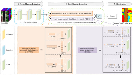
Figure 1. Overview illustration of the proposed MSLKACNN, which consists of two primary blocks, i.e., a spectral feature extraction module (SFEM) and a multi-scale large kernel asymmetric convolution (MSLKAC) block. MSLKAC includes three key components: MLKADC, MADDC, and an average fusion pooling (AFP).

(1) We introduce a novel MLKADC to extract local-to-global spatial features. The MLKADC utilizes a series of asymmetric DWCs with small to large kernels, addressing the limitations of existing DL models. Notably, it extends the non-square kernel sizes to $1\times 17$ and $17\times 1$, thus enhancing the global feature extraction capabilities while reducing the number of parameters compared to SSLKA, which relies on standard square kernels.

(2) We propose a new MADDC to model the spatial relationships between land covers at different distances by combining ADC with dilated convolution.

(3) By combining the proposed MLKADC and MADDC in parallel, we develop a novel MSLKAC for improving the ability to extract spatial features across small to large ranges. Based on our MSLKAC, we introduce an architecture termed MSLKACNN to jointly learn both spectral and spatial features through the SFEM and MSLKAC.

The rest of the paper is organized as follows. In Section 2, we present the related works of HSI classification models. The proposed MSLKACNN is introduced in Section 3. In Section 4, we evaluate and discuss the performance of MSLKACNN. We summarize the paper in Section 5.

2. Related Work

HSI classification methods are typically categorized into traditional ML-based approaches and DL-based approaches. DL-based approaches mainly comprise five types of models: CNN-based models, GCN-based models, Transformer-based models, Mamba-based models, and LKCNN-based models.

(1) ML-based models: In early studies, traditional ML methods, such as Markov random fields [7] and morphological profiles [44], tend to be applied in HSI classification. These models heavily rely on manual design and exhibit limited learning ability in extracting deep semantic features from HSI [31].

(2) CNN-based models: Many CNN-based models, ranging from 1D-CNN [45] to 2D-CNN [46] and 3D-CNN [14], have been applied to capture features from HSI in an end-to-end manner. Additionally, channel-based CNN frameworks, including single-channel CNN [46], dual-channel CNN [47], and multi-channel CNN [48], have been employed to learn spatial–spectral features. Zhong et al. [49] and Wang et al. [21] respectively introduce residual connections [50] and dense connections [51] into their CNNs to significantly deepen their models, addressing the degradation [50] of deep CNNs. Nevertheless, the majority of these models are limited to extracting features at a single scale from fixed-size image patches, resulting in suboptimal and unstable results under complex HSI with limited training samples [52,53]. To tackle these issues, numerous works establish multi-scale CNN architectures to capture multi-scale features. For instance, Gong et al. [54] design a novel multi-scale CNN to more effectively learn features compared with single-scale CNN methods. MMFN [22] combines the complementary and related features at different scales to achieve optimal results. To boost the learning capability for extracting spatial–spectral features, attention-based CNN models have been explored. Li et al. [8] introduce a new double-branch dual-attention approach termed DBDA, which designs a channel attention block and a spatial attention block to enhance classification performance. Roy et al. [24] introduce efficient feature recalibration (EFR) into improved 3D residual blocks to adjust the size of the receptive field and enhance cross-channel relationships. Furthermore, Wang et al. [23] develop a novel attention-based multi-scale CNN architecture to better capture pixel-level discriminative features. These CNN-based models typically contain multiple small convolutional kernels, thus excelling at extracting local spatial–spectral features. However, they have difficulty in modeling the long-range dependencies between land covers because of the inherent locality of their small kernel convolutions.

(3) GCN-based models: Leveraging the capability of GCNs to capture spatial relationships ranging from short range to long range, they have been extensively utilized in HSI classification tasks. Qin et al. [17] present a spectral–spatial GCN by establishing each pixel of HSI as a graph node. Subsequently, Bai et al. [18] propose attention GCN frameworks to capture the non-Euclidean features of HSI. The aforementioned GCN models treat each pixel in HSI as a graph node, leading to tremendous computations. To overcome the limitation, many works explore superpixel-based GCNs that use superpixels instead of pixels as graph nodes [55,56]. For example, Wang et al. [56] significantly reduce the computational complexity by constructing a superpixel graph, which facilitates GCNs to deal with large HSI data. Nevertheless, for these superpixel-based networks, the features of pixels are shared among each superpixel, thereby inevitably overlooking the individual characteristics of these pixels. This neglects the results with limited classification accuracy. To address these limitations, CNN and GCN fusion-based frameworks have been introduced [28,29,57]. These fusion models fully leverage the advantages of their CNNs and GCNs, jointly mining features at both the pixel level and superpixel level to achieve complementary feature extraction. However, these models struggle with classifying large-scale HSI data, due to the complex computations and memory costs incurred by graph construction.

(4) Transformer-based models: Researchers have successfully applied Transformer to HSI classification. For instance, He et al. [58] and Hong et al. [19] propose Transformer-based approaches, employing the multi-head self-attention (MHSA) [59] mechanism to model long-range relationships across different land cover types. In addition to these single Transformer structures, several fusion architectures have been developed. SSFTT [10] captures low-level and high-level features through two convolutional layers and a Gaussian weighted feature tokenizer, respectively, before establishing global information with a Transformer. Subsequently, Zhao et al. [32] present a lightweight groupwise separable convolutional vision Transformer network (GSCViT), utilizing groupwise separable convolutions and groupwise separable MHSA blocks to extract both local and global features. Furthermore, several works, such as MVAHN [60] and GTFN [31], explore the fusion of Transformers with GCNs to leverage the strengths of both models, thereby enhancing classification performance. Although these models effectively model long-term dependencies, they suffer from challenges in terms of speed and memory usage in large-scale HSI, owing to the quadratic computational complexity of Transformer.

(5) Mamba-based models: Recently, several Mamba models [20,34,61] have been explored for HSI classification. SpectralMamba [34] adopts Mamba to capture global information and model long-range relationships, achieving linear computational complexity. Zhou et al. [61] present Mamba-in-Mamba architecture to extract global features, which is more efficient in computation than Transformer-based models. Furthermore, Li et al. [20] design spatial and spectral Mamba blocks to extract spatial and spectral features. Although these models excel in long-range modeling and maintain linear computational complexity, they necessitate enhanced local feature extraction capabilities.

(6) LKCNN-based models: Motivated by the success of LKCNN models in natural visual tasks, several works utilize LKCNNs to extract the long-range features of HSI [39,40,41]. LiteCCLKNet [39] employs the criss-cross large kernel module to learn global information. LKSSAN [40] and SSLKA [41] apply large kernel attention (LKA) [37], which consists of depthwise convolution (DWC), depthwise dilation convolution (DDC), and pointwise convolution (PWC), to extract long-range features. To enhance the both local and global feature extraction capabilities of these large kernel networks while significantly reducing their parameter size and computational complexity, we design a new multi-scale large kernel asymmetric CNN (MSLKACNN). Unlike LKSSAN and SSLKA that use a sequence of DWC, DDC, and PWC to capture global features, our MSLKACNN captures both local and global spatial features while improving computational efficiency and reducing the number of parameters by employing two parallel multi-scale asymmetric convolution components: (1) the proposed MLKADC that constructs asymmetric DWCs ranging from a sequence of two DWCs with $1\times 3$ and $3\times 1$ kernels to a sequence of two DWCs with $1\times m$ and $m\times 1$ kernels, for extracting small local, larger local, and global spatial features; and (2) the proposed MADDC, which extracts spatial information among pixels at varying distances via multi-scale learning and asymmetric dilated DWCs.

3. Proposed Method

The flowchart of the proposed MSLKACNN architecture is depicted in Figure 1, comprising two blocks and a classifier: (1) a spectral feature extraction module (SFEM), designed to eliminate noise, reduce the dimensionality of bands, and learn spectral features in raw HSI data; (2) a multi-scale large kernel asymmetric convolution (MSLKAC), which utilizes two parallel multi-scale asymmetric convolutions with small to large kernels to capture both local and global spatial features; and (3) a Softmax classifier that assigns labels to individual pixels.

3.1. SFEM

The original HSI data incorporate superfluous spectral information and are prone to being influenced by noise. To circumvent these issues and extract spectral features, we design the SFEM. Unlike principal component analysis (PCA), which applies linear transformations to hyperspectral data for dimensionality reduction, our SFEM automatically performs nonlinear operations to reduce the dimensionality of HSI through three consecutive identical convolutional blocks equipped with a limited number of filters, suppressing noise and learning the spectral features of the hyperspectral data. Each block in the proposed SFEM consists of a $1\times 1$ convolution, a batch normalization (BN), and a ReLU6 function.

Let $X^l$ be the input feature map of the l-th convolutional layer, and the output feature map of the convolutional layer, denoted as $X^{l+1}$, can be expressed as

$$X^{l+1}=\mathrm{ReLU}6\left(\mathrm{BN}\left({\mathrm{Conv}1}^l\left(X^l\right)\right)\right),$$

(1)

where ${\mathrm{Conv}1}^l$ represents the l-th convolutional layer with a $1\times 1$ kernel.

3.2. MSLKAC

In this section, we introduce the innovative MSLKAC, which enlarges the large kernel sizes to $1\times 17$ and $17\times 1$ as illustrated in Figure 1. The MSLKAC consists of two convolutions and a fusion operation: (1) a multi-scale large kernel asymmetric depthwise convolution (MLKADC), which employs techniques such as multi-scale learning and asymmetric depthwise convolutions with small to large kernels, to extract spatial features from HSI data across various ranges; (2) a multi-scale asymmetric dilated depthwise convolution (MADDC) that captures spatial information among pixels at varying distances by combining these techniques, including multi-scale learning, dilated convolutions, depthwise convolutions, and asymmetric convolutions; and (3) an average fusion pooling (AFP) that integrates the features learned by the two convolutions. The details of these three components will be described in the following sections.

(1) Multi-Scale Large Kernel Asymmetric Depthwise Convolution (MLKADC): Compared with an ordinary convolution, DWC considerably reduces the computational complexity and the number of parameters by convolving each channel of the input feature map separately. Due to these advantages of DWC, Gao et al. [62] use DWCs instead of ordinary convolutions to learn spectral features from HSI. For the further reduction in the number of computations and parameters, we design a new asymmetric depthwise convolution (ADC) as illustrated in Figure 2b. In the proposed ADC, we decompose a $3\times 3$ DWC (with a kernel size of $3\times 3$, as shown in Figure 2a) into a $1\times 3$ DWC and a $3\times 1$ DWC, with the goal of improving the computational efficiency and reducing the number of parameters. To extract small local, larger local, and global spatial features from HSI, we present a novel MLKADC by constructing ADCs ranging from a sequence of two DWCs with $1\times 3$ and $3\times 1$ kernels to a sequence of two DWCs with $1\times m$ and $m\times 1$ kernels as depicted in Figure 2c. The proposed MLKADC comprises $(m-1)/2$ parallel ADCs. These ADCs take the same input information as captured by SFEM, perform convolution operations in an equal-width manner, maintain a consistent topology, and adhere to two rules: (i) these hyperparameters (filter numbers, strides) remain the same across these ADCs, except for their varying kernel sizes; and (ii) the kernel sizes are distributed in an arithmetic progression with a common difference of 2. Following these two rules, we merely need to design the first template ADC and establish the scale numbers, and our MLKADC can be determined accordingly. Consequently, these two rules significantly streamline the design space, allowing us to concentrate on optimizing a few hyperparameters.

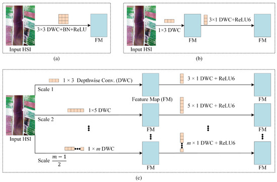
Figure 2. Different depthwise convolutions. (a) Depthwise convolution. (b) Proposed asymmetric depthwise convolution. (c) Proposed multi-scale large kernel asymmetric depthwise convolution (MLKADC).

For the proposed MLKADC, we utilize DWCs with various kernels ranging from $1\times 3$ to $1\times m$ to extract spatial features along the width of HSI, followed by DWCs and ReLU6 functions with diverse kernels ranging from $3\times 1$ to $m\times 1$ to learn spatial features along the height of HSI, where $1\times m$ and $m\times 1$ represent the largest kernel sizes in the width and height directions, respectively. As m is set to a large value of 17 in our experiments, we refer to our MLKADC as a large kernel convolution. We take the feature map $X_p$ learned by our SFEM as the input, then its output feature map $H_{\mathrm{MLKADC}}$ can be defined as

$$H_{\mathrm{MLKADC}}=\mathrm{MLKADC}\left(X_p\right)=\{{\tilde{H}}_3,{\tilde{H}}_5,\dots ,{\tilde{H}}_m\},$$

(2)

where ${\tilde{H}}_m$ represents the extracted features from $X_p$ through a sequence consisting of a DWC with a $1\times m$ kernel, a DWC with an $m\times 1$ kernel, and a ReLU6 activation function.

In our MLKADC, we employ a sequence of asymmetric convolutions with small kernels (e.g., $1\times 3$ and $3\times 1$) to learn local spatial features, utilize asymmetric convolutions with medium-sized kernels (such as $1\times 7$ and $7\times 1$) for the extraction of larger local spatial features, and use a sequence of asymmetric convolutions with large kernels (like $1\times 17$ and $17\times 1$) to capture global spatial features.

(2) Multi-Scale Asymmetric Dilated Depthwise Convolution (MADDC): Dilated convolution can effectively enlarge the receptive field of ordinary convolutions while avoiding the introduction of additional parameters. Owing to these advantages, dilated convolution has been explored and achieved competitive classification performance in HSI classification [63]. This inspires us to introduce dilated convolution into our model. To simultaneously employ the benefits of dilated convolution and DWC, we construct a $3\times 3$ dilated depthwise convolution (DDC) with a dilation factor $d=2$ by combining these two convolutions (Figure 3a). To improve the computational efficiency and achieve reduction in the parameters, we design an asymmetric dilated depthwise convolution (ADDC) comprising three consecutive components: a $1\times 3$ DDC with $d=2$, a $3\times 1$ DDC with $d=2$, and a ReLU6 function as shown in Figure 3b. To enhance the capability of spatial feature extraction, we propose a novel MADDC by utilizing $(k-1)/2$ ADDCs with kernels ranging from $1\times 3$ and $3\times 1$ to $1\times k$ and $k\times 1$ as depicted in Figure 3c. These ADDCs carry out convolution operations in an equal-width manner, maintaining a similar structure. They are simplified by two rules: (i) apart from varying kernel sizes and dilation factors, the other hyperparameters (filter numbers and strides) are set to be the same; and (ii) the spatial sizes and dilation factors are arranged in arithmetic progressions with common differences of 2 and 1, respectively. Analogous to our MLKADC, according to the two rules, we only need to design the first template ADDC and set the scale numbers, and they can be determined accordingly. Hence, our MADDC avoids complicated design.

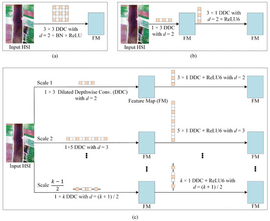
Figure 3. Various dilated depthwise convolutions. (a) Proposed dilated depthwise convolution. (b) Proposed asymmetric dilated depthwise convolution. (c) Proposed multi-scale asymmetric dilated depthwise convolution (MADDC).

As illustrated in Figure 3c, these DDCs with different kernels ranging from $1\times 3$ to $1\times k$, are used to learn spatial information across the width of HSI. Then, these DDCs with diverse kernels ranging from $3\times 1$ to $k\times 1$, combined with ReLU6 functions, are designed to capture spatial features along the height of HSI, where $1\times k$ and $k\times 1$ denote the largest kernel sizes in the width and height directions for the proposed MADDC, respectively. Let $H_{\mathrm{MADDC}}$ denote the output features of MADDC, then we have

$$H_{\mathrm{MADDC}}=\mathrm{MADDC}\left(X_p\right)=\{{\widehat{H}}_3,{\widehat{H}}_5,\dots ,{\widehat{H}}_k\},$$

(3)

where ${\widehat{H}}_k$ represents the learned features from $X_p$ through a sequence of three operations: a $1\times k$ DDC with $d=(k+1)/2$, a $k\times 1$ DDC with $d=(k+1)/2$, and a ReLU6 function.

In our MADDC, we employ parallel ADDCs with various kernels and dilation factors to capture spatial features and model the relationships between pixels at diverse distances.

(3) Average Fusion Pooling (AFP): The proposed MSLKAC consists of two parallel asymmetric convolutions: (1) MLKADC that is utilized to learn small local, larger local, and global spatial features; and (2) MADDC that is used to extract spatial information at various distances. To integrate these features learned by the two convolutions, we explore a fusion scheme named average fusion pooling (AFP). Let $H_{\mathrm{MSLKAC}}$ represent the output features of AFP. With Equations (2) and (3), the AFP can be expressed as

$$\begin{array}{cc}\hfill H_f& =\mathrm{AFP}(H_{\mathrm{MLKADC}};H_{\mathrm{MADDC}})\hfill \\ \hfill & ={\displaystyle \frac{1}{s}}\left({\tilde{H}}_3+{\tilde{H}}_5+\cdots +{\tilde{H}}_m+{\widehat{H}}_3+{\widehat{H}}_5+\cdots +{\widehat{H}}_k\right),\hfill \end{array}$$

(4)

where $s=(m+k-2)/2$ is the total number of scales in the proposed MSLKAC. In HSI classification tasks, common fusion schemes typically include column concatenation [9] and sum [60]. Under the large value s, our AFP offers the following advantages: (1) In contrast to column concatenation fusion, the number of parameters in AFP is significantly reduced, thus mitigating the risk of overfitting; and (2) AFP effectively addresses the potential issue of large features resulting from sum operation, thereby preventing the concern of gradient explosion.

3.3. Softmax Classification

After AFP, to determine the label of each pixel, we utilize a Softmax classifier to classify the fused feature map $H_{\mathrm{MSLKAC}}$. We have

$$Y={\displaystyle \frac{e^{W_i{H}_{\mathrm{MSLKAC}}+b_i}}{{\sum }_i^c{e}^{W_i{H}_{\mathrm{MSLKAC}}+b_i}}},$$

(5)

where c represents the number of land cover categories, and $W_i$ and $b_i$ denote the trainable parameter and bias. We adopt a cross-entropy error as the loss function to train our model, namely,

$$\mathcal{L}=-\sum _{Z\in O_{\mathrm{label}}}\sum _{j=1}^c{O}_{zj}ln{Y}_{zj},$$

(6)

where O represents the label matrix, and $Y_{zj}$ denotes the probability of the z-th pixel belonging to the j-th category.

4. Experiment

In this section, we first describe four publicly available benchmark HSI datasets. Then, we introduce the evaluation metrics, compared methods, and implementation details. Next, we qualitatively and quantitatively assess the performance of the proposed MSLKACNN and state-of-the-art methods. Subsequently, we compare different training samples and fusion schemes, as well as training and testing times across various methods. Finally, we conduct several ablation studies to analyze the impacts of key components and hyperparameters.

4.1. Dataset Description

In our experiments, the four HSI datasets are Indian Pines, Botswana, Houston 2013, and WHU-Hi-LongKou (LongKou), respectively. We summarize the details of these datasets in Table 1 and Table 2.

Table 1. Summary of Indian Pines and Botswana datasets. No. denotes number. Train., Val., and Test. represent the number of training samples, validation samples, and test samples, respectively.

Dataset	Indian Pines				Botswana
Wavelength	0.4–2.5 μm				0.4–2.5 μm
Data Size	145 × 145 × 200				1476 × 256 × 145
Time	1992				2001
Class No.	Class Name	Train.	Val.	Test.	Class Name	Train.	Val.	Test.
C1	Alfalfa	2	5	39	Water	2	5	263
C2	Corn-notill	2	5	1421	Hippo Grass	2	5	94
C3	Corn-mintill	2	5	823	Floodplain Grasses 1	2	5	244
C4	Corn	2	5	230	Floodplain Grasses 2	2	5	208
C5	Grass-pasture	2	5	476	Reeds	2	5	262
C6	Grass-trees	2	5	723	Riparian	2	5	262
C7	Grass-pasture-mowed	2	5	21	Fires Car	2	5	252
C8	Hay-windrowed	2	5	471	Island Interior	2	5	196
C9	Oats	2	5	13	Acacia Woodlands	2	5	307
C10	Soybean-notill	2	5	965	Acacia Shrub Lands	2	5	241
C11	Soybean-mintill	2	5	2448	Acacia Grasslands	2	5	298
C12	Soybean-clean	2	5	589	Short Mopane	2	5	174
C13	Wheat	2	5	198	Mixed Mopane	2	5	261
C14	Woods	2	5	1258	Exposes Soils	2	5	88
C15	Buildings-Grass-Trees-Drives	2	5	379	-	-	-	-
C16	Stone-Steel-Towers	2	5	86	-	-	-	-
Total	-	32	80	10,137	-	28	70	3150

Table 2. Summary of Houston 2013 and LongKou datasets. No. denotes number. Train., Val., and Test. represent the number of training samples, validation samples, and test samples, respectively.

Dataset	Houston 2013				LongKou
Wavelength	0.38–1.05 μm				0.4–1.0 μm
Data Size	349 × 1905 × 144				550 × 400 × 270
Time	2013				2018
Class No.	Class Name	Train.	Val.	Test.	Class Name	Train.	Val.	Test.
C1	Healthy Grass	2	5	1244	Corn	2	5	34,504
C2	Stressed Grass	2	5	1247	Cotton	2	5	8367
C3	Synthetic Grass	2	5	690	Sesame	2	5	3024
C4	Tree	2	5	1239	Broad-Leaf Soybean	2	5	63,205
C5	Soil	2	5	1235	Narrow-Leaf Soybean	2	5	4144
C6	Water	2	5	318	Rice	2	5	11,847
C7	Residential	2	5	1261	Water	2	5	67,049
C8	Commercial	2	5	1237	Roads and Houses	2	5	7117
C9	Road	2	5	1245	Mixed Weed	2	5	5222
C10	Highway	2	5	1220	-	-	-	-
C11	Railway	2	5	1228	-	-	-	-
C12	Parking Lot 1	2	5	1226	-	-	-	-
C13	Parking Lot 2	2	5	462	-	-	-	-
C14	Tennis Court	2	5	421	-	-	-	-
C15	Running Track	2	5	653	-	-	-	-
Total	-	30	75	14,924	-	18	45	204,479

(1) Indian Pines: The Indian Pines dataset was acquired by the Airborne Visible Infrared Imaging Spectrometer sensor in 1992. It contains 10,249 labeled pixels with 16 ground-truth classes, consisting of $145\times 145$ pixels in the wavelength range from 0.4 to 2.5 μm. After removing these noisy and water absorption bands of 104–108, 150–163, and 220, 200 spectral bands are retained.

(2) Botswana: The Botswana dataset was captured by using the NASA EO-1 satellite over the Okavango Delta region in Botswana. The whole image comprises $1476\times 256$ pixels with 242 spectral bands, 14 land cover categories, and wavelengths ranging from 0.4 to 2.5 μm. We retain 145 spectral bands by removing 97 noise bands.

(3) Houston 2013: The Houston 2013 dataset was provided by the National Center for Airborne Laser Mapping (NCALM) over the University of Houston in 2013 [64]. The dataset contains 15,029 labeled pixels with 16 land cover categories, comprising $349\times 1905$ pixels with 144 spectral bands ranging from 0.38 to 1.05 μm.

(4) WHU-Hi-LongKou (LongKou): The LongKou dataset was gathered by using an 8 mm focal length Headwall Nano-Hyperspec imaging sensor over the town of LongKou, Hubei Province, China in 2018 [65]. The HSI consists of $550\times 400$ pixels with 9 land cover classes and 240 spectral bands in the wavelength range from 0.4 to 1.0 μm.

4.2. Experimental Setup

(1) Evaluation Metrics: To quantitatively analyze the effectiveness of the proposed MSLKACNN, four evaluation metrics are introduced: per-class accuracy, overall accuracy (OA), average accuracy (AA), and Kappa coefficient (KAPPA). Furthermore, the classification maps produced by various models are visualized to enable a qualitative assessment.

(2) Comparison Methods: To demonstrate the strengths of the proposed MSLKACNN, ten comparison methods are selected and evaluated. These comparison methods are divided into four categories, including (a) CNN-based methods: the double-branch dual-attention network (DBDA) [8], and the attention-based adaptive spectral–spatial kernel ResNet ($A^2{S}^{2}K-\mathrm{Res}$) [24]; (b) GCN-based methods: the CNN-enhanced GCN (CEGCN) [9], the fast dynamic graph convolutional network and CNN parallel network (FDGC) [27], and the GCN and transformer fusion network (GTFN) [31]; (c) Transformer-based methods: the spectral–spatial feature tokenization transformer (SSFTT) [10], the groupwise separable convolutional vision Transformer (GSC-ViT) [32], and the double branch convolution-transformer network (DBCTNet) [33]; (d) Mamba-based method: the spatial–spectral Mamba (MambaHSI) [20]; and (e) LKCNN-based method: the spectral–spatial large kernel attention network (SSLKA) [41].

(3) Implementation Details: All experiments are implemented on a Silver 4210 CPU, Python 3.10, and a GTX-3090 GPU. We adopt the Adam optimizer with a learning rate of 0.001 on the Pytorch platform. In the proposed MSLKACNN, the number of filters for all convolutional layers is set to 64. For our MSLKAC, we set the large kernel size m in MLKADC to 17 while setting the kernel size k in MADDC to 5. We train our model for 200 epochs on the Botswana, for 120 epochs on the Houston 2013, and for 150 epochs on the other datasets. All experiments of our MSLKACNN and the comparison methods are repeated twenty times with various random initializations, and the average results are reported across each evaluation metric.

4.3. Comparison with State-of-the-Art Methods

In this section, we conduct a quantitative and qualitative evaluation between the proposed MSLKACNN and existing state-of-the-art baselines on the Indian Pines, Botswana, Houston 2013, and LongKou datasets. These baselines are implemented using the optimal parameters as described in their respective references.

(1) Results on Indian Pines: Table 3 shows the quantitative comparison of all methods on the Indian Pines dataset. From the table, we observe that our MSLKACNN outperforms almost all baselines (except for MambaHSI in KAPPA) in terms of OA, AA, and KAPPA, as well as seven out of sixteen land cover categories. Specifically, MSLKACNN improves over CNN approaches by at least 7.92%, improves over GCN approaches by at least 24.06%, improves over Transformer approaches by at least 21.15%, improves over the Mamba approach by 24.56%, and improves over the LKCNN approach by 15.84% in terms of OA, respectively. These improvements highlight the superiority of the proposed MSLKACNN.

Table 3. Quantitative comparison of all methods on the Indian Pines dataset using two labeled samples per class for training.

Class	CNNs		GCNs			Transformers			Mamba	LKCNN
	DBDA	${\mathit{A}}^{\mathbf{2}}{\mathit{S}}^{\mathbf{2}}\mathit{K}$-Res	CEGCN	FDGC	GTFN	SSFTT	GSC-ViT	DBCTNet	MambaHSI	SSLKA	MSLKACNN
	RS 2020	TGRS 2021	TGRS 2021	TGRS 2022	TGRS 2023	TGRS 2022	TGRS 2024	TGRS 2024	TGRS 2024	TGRS 2024	Ours
1	98.46 ± $2.05$	96.67 ± $4.14$	68.21 ± $19.30$	95.38 ± $8.79$	90.91 ± $9.14$	100.0 ± 0.00	78.72 ± $21.24$	87.18 ± $13.37$	93.59 ± $3.85$	95.38 ± $3.20$	98.97 ± $2.35$
2	38.99 ± $16.71$	30.61 ± $15.52$	36.74 ± $17.84$	29.58 ± $12.94$	40.86 ± $9.80$	32.78 ± $2.93$	27.34 ± $13.12$	27.97 ± $12.00$	33.53 ± $11.29$	25.38 ± $4.92$	51.97 ± 10.84
3	37.40 ± $13.27$	25.82 ± $12.87$	38.31 ± $20.29$	35.39 ± $8.48$	35.58 ± $12.17$	54.46 ± 6.46	42.24 ± $13.92$	31.19 ± $9.49$	41.04 ± $16.68$	30.52 ± $8.23$	43.24 ± $16.59$
4	88.13 ± $11.79$	59.87 ± $22.14$	37.61 ± $16.95$	83.83 ± $17.19$	73.49 ± $20.01$	82.70 ± $3.67$	64.43 ± $16.30$	65.70 ± $19.72$	67.87 ± $21.62$	90.17 ± 8.96	85.78 ± $9.92$
5	53.24 ± $23.30$	61.87 ± $21.49$	56.24 ± $15.79$	59.79 ± $12.01$	52.37 ± $23.34$	13.51 ± $3.95$	60.29 ± $19.49$	53.38 ± $15.82$	50.74 ± $26.73$	60.27 ± $3.57$	64.37 ± 16.78
6	95.44 ± $2.64$	90.22 ± $10.40$	78.42 ± $24.16$	74.27 ± $12.94$	82.18 ± $9.98$	93.13 ± $2.49$	82.70 ± $9.54$	83.42 ± $9.86$	81.42 ± $13.89$	98.70 ± 1.16	95.39 ± $3.52$
7	100.0 ± 0.00	100.0 ± 0.00	87.14 ± $11.08$	100.0 ± 0.00	99.23 ± $1.54$	100.0 ± 0.00	100.0 ± 0.00	100.0 ± 0.00	97.62 ± $4.39$	100.0 ± 0.00	100.0 ± 0.00
8	73.14 ± $24.93$	53.50 ± $20.03$	59.34 ± $20.98$	83.29 ± $8.50$	80.86 ± $12.69$	96.41 ± 2.50	74.48 ± $26.43$	65.50 ± $18.60$	77.88 ± $16.75$	55.56 ± $14.88$	91.66 ± $15.30$
9	100.0 ± 0.00	93.85 ± $9.61$	82.31 ± $17.22$	96.92 ± $7.05$	93.89 ± $5.24$	100.0 ± 0.00	99.23 ± $2.31$	98.46 ± $4.62$	99.23 ± $2.31$	100.0 ± 0.00	100.0 ± 0.00
10	45.23 ± $22.16$	30.60 ± $22.23$	60.52 ± $22.12$	48.41 ± $17.60$	49.87 ± $11.87$	53.14 ± $7.20$	48.41 ± $15.12$	43.23 ± $19.43$	50.39 ± $14.95$	47.84 ± $5.56$	70.15 ± 9.87
11	57.99 ± 12.34	49.24 ± $15.66$	35.97 ± $20.93$	40.69 ± $17.78$	39.32 ± $13.68$	38.74 ± $7.85$	48.30 ± $14.92$	40.11 ± $18.04$	39.87 ± $18.54$	51.56 ± $7.04$	55.35 ± $13.16$
12	48.40 ± $10.22$	41.14 ± $20.58$	26.55 ± $13.50$	34.78 ± $13.61$	42.74 ± $15.98$	40.44 ± $4.29$	31.38 ± $4.68$	25.67 ± $6.40$	32.80 ± $8.55$	60.60 ± 5.63	52.95 ± $12.02$
13	99.90 ± 0.30	89.90 ± $24.37$	97.93 ± $5.07$	97.02 ± $3.80$	94.93 ± $2.86$	96.21 ± $2.27$	99.39 ± $0.87$	96.36 ± $5.42$	98.69 ± $3.13$	97.88 ± $2.81$	99.75 ± $0.61$
14	93.24 ± 4.90	63.80 ± $17.90$	69.27 ± $20.21$	76.45 ± $11.01$	74.20 ± $11.66$	79.89 ± $5.39$	70.36 ± $10.35$	82.98 ± $9.96$	80.78 ± $9.62$	91.34 ± $2.36$	83.37 ± $10.49$
15	75.20 ± $17.41$	47.92 ± $13.91$	36.52 ± $15.49$	61.08 ± $16.07$	63.15 ± $19.46$	71.13 ± $4.97$	48.89 ± $15.77$	65.59 ± $14.67$	73.03 ± $21.86$	56.73 ± $7.67$	89.60 ± 12.70
16	100.0 ± 0.00	97.67 ± $4.85$	98.26 ± $2.81$	95.93 ± $8.16$	96.70 ± $5.96$	100.0 ± 0.00	99.19 ± $2.08$	98.95 ± $1.51$	97.79 ± $3.47$	100.0 ± 0.00	99.88 ± $0.35$
OA	62.21 ± $5.90$	49.75 ± $3.02$	49.34 ± $4.72$	52.52 ± $5.77$	54.12 ± $4.28$	55.42 ± $2.27$	52.98 ± $5.22$	50.87 ± $4.05$	53.90 ± $4.61$	57.96 ± $1.50$	67.14 ± 2.50
AA	75.30 ± $4.19$	64.54 ± $3.96$	60.58 ± $3.64$	69.55 ± $2.62$	69.39 ± $4.18$	72.03 ± $1.06$	67.21 ± $2.72$	66.61 ± $2.45$	69.77 ± $4.08$	72.62 ± $1.44$	80.15 ± 1.70
KAPPA	57.47 ± $6.52$	43.78 ± $3.85$	43.64 ± $4.70$	47.78 ± $5.92$	49.33 ± $4.52$	50.58 ± $2.31$	47.57 ± $5.29$	45.44 ± $3.86$	68.13 ± 5.25	52.90 ± $1.15$	63.30 ± $2.64$

Figure 4 illustrates a qualitative evaluation through the visualization of classification maps obtained by various methods on the Indian Pines dataset. These maps clearly show that the proposed MSLKACNN exhibits fewer misclassifications in many classes, such as “Corn-notill” and “Soybean-notill”, in comparison to other methods.

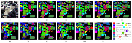
Figure 4. False-color image, ground truth, and classification maps on the Indian Pines dataset. (a) False-color image. (b) Ground truth. (c) DBDA (OA = 62.21%). (d) $A^2{S}^{2}K\text{-}\mathrm{Res}$ (OA = 49.75%). (e) CEGCN (OA = 49.34%). (f) FDGC (OA = 52.52%). (g) GTFN (OA = 54.12%). (h) SSFTT (OA = 55.42%). (j) GSC-ViT (OA = 52.98%). (k) DBCTNet (OA = 50.87%). (l) MambaHSI (OA = 53.90%). (m) SSLKA (OA = 57.96%). (i) MSLKACNN (OA = 67.14%).

(2) Results on Botswana: The comparative results of various approaches on the Botswana dataset are summarized in Table 4. The results reveal two key findings: (a) Among all methods, the GSC-ViT, MambaHSI, SSLKA, and CEGCN models achieve the third-best, fourth-best, fifth-best, and sixth-best performance in terms of OA and AA, respectively. This is mainly due to the fact that these models can effectively establish long-range dependencies within the HSI data by utilizing Transformer, Mamba, LKCNN, and GCN, respectively. (b) Our MSLKACNN, which employs multi-scale asymmetric convolutions with kernels ranging from small to large, excels in capturing global features that are neglected by traditional CNNs, performing better than baseline methods in evaluation metrics, including OA, AA, and KAPPA. Specifically, in terms of OA, AA, and KAPPA, MSLKACNN outperforms GTFN by 15.79%, 15.13%, and 17.11%, respectively; outperforms DBCTNet by 6.99%, 6.39%, and 7.57%, respectively; outperforms MambaHSI by 4.41%, 4.15%, and 6.76%, respectively; and outperforms SSLKA by 4.75%, 5.66%, and 5.16%, respectively. These findings further validate the effectiveness of MSLKACNN.

Table 4. Quantitative comparison of all methods on the Botswana dataset using two labeled samples per class for training.

Class	CNNs		GCNs			Transformers			Mamba	LKCNN
	DBDA	${\mathit{A}}^{\mathbf{2}}{\mathit{S}}^{\mathbf{2}}\mathit{K}$-Res	CEGCN	FDGC	GTFN	SSFTT	GSC-ViT	DBCTNet	MambaHSI	SSLKA	MSLKACNN
	RS 2020	TGRS 2021	TGRS 2021	TGRS 2022	TGRS 2023	TGRS 2022	TGRS 2024	TGRS 2024	TGRS 2024	TGRS 2024	Ours
1	99.92 ± $0.23$	94.45 ± $10.01$	96.46 ± $6.10$	71.83 ± $18.94$	84.85 ± $11.80$	35.02 ± $12.13$	99.47 ± $1.24$	98.17 ± $3.74$	100.0 ± 0.00	100.0 ± 0.00	95.13 ± $6.33$
2	100.0 ± 0.00	95.85 ± $11.10$	99.36 ± $0.98$	91.91 ± $13.00$	89.60 ± $16.17$	100.0 ± 0.00	98.72 ± $3.18$	99.15 ± $1.95$	89.15 ± $17.97$	99.04 ± $1.93$	100.0 ± 0.00
3	98.69 ± $3.67$	83.03 ± $14.51$	84.06 ± $21.00$	72.46 ± $19.32$	80.76 ± $9.38$	79.26 ± $3.78$	88.48 ± $9.94$	81.68 ± $16.64$	98.61 ± $1.29$	98.93 ± 1.46	93.89 ± $8.64$
4	97.98 ± $5.74$	90.34 ± $20.20$	96.97 ± $8.93$	80.38 ± $24.90$	85.92 ± $16.11$	100.0 ± 0.00	97.60 ± $3.04$	96.97 ± $5.16$	97.98 ± $3.89$	97.45 ± $5.31$	95.19 ± $10.65$
5	65.11 ± $23.17$	73.40 ± $17.44$	50.80 ± $19.73$	66.56 ± $16.44$	58.69 ± $12.34$	65.38 ± $7.27$	75.50 ± $13.56$	66.95 ± $15.70$	66.34 ± $14.80$	96.76 ± 2.80	85.69 ± $10.70$
6	81.11 ± $15.00$	63.59 ± $19.80$	52.86 ± $10.67$	59.47 ± $16.87$	40.22 ± $13.37$	51.60 ± $5.40$	66.07 ± $24.54$	56.91 ± $20.20$	61.11 ± $16.57$	40.15 ± $6.94$	86.95 ± 10.52
7	99.92 ± $0.24$	99.60 ± $1.19$	96.15 ± $6.29$	94.13 ± $6.34$	93.50 ± $7.46$	97.82 ± $4.45$	99.29 ± $1.30$	99.84 ± $0.19$	98.13 ± $4.47$	100.0 ± 0.00	98.53 ± $3.68$
8	77.45 ± $16.06$	66.73 ± $23.63$	88.11 ± $21.69$	66.99 ± $28.17$	76.67 ± $18.03$	99.90 ± 0.31	90.46 ± $13.00$	75.26 ± $19.41$	91.28 ± $9.64$	62.04 ± $4.84$	86.58 ± $12.00$
9	84.17 ± $28.12$	87.62 ± $12.60$	95.15 ± $13.61$	83.52 ± $18.97$	81.57 ± $12.54$	93.88 ± $6.73$	89.67 ± $8.68$	90.49 ± $16.93$	82.28 ± $14.72$	100.0 ± 0.00	95.57 ± $6.50$
10	89.21 ± $13.40$	77.05 ± $23.88$	94.19 ± $13.59$	82.16 ± $22.18$	77.32 ± $19.61$	74.90 ± $11.27$	89.63 ± $19.40$	79.75 ± $19.49$	97.22 ± $4.23$	99.21 ± 1.04	90.33 ± $18.43$
11	94.60 ± $6.63$	79.09 ± $20.62$	90.20 ± $8.89$	72.89 ± $17.94$	70.53 ± $23.92$	96.71 ± 3.96	89.77 ± $12.56$	87.48 ± $11.56$	79.93 ± $20.01$	68.52 ± $3.55$	86.21 ± $10.09$
12	96.72 ± $4.71$	71.26 ± $22.98$	97.99 ± $4.09$	63.85 ± $17.91$	79.78 ± $18.54$	79.60 ± $4.26$	99.20 ± 0.90	85.11 ± $14.68$	96.21 ± $4.96$	97.47 ± $1.24$	95.98 ± $8.28$
13	99.39 ± $1.36$	92.87 ± $13.92$	99.12 ± $2.00$	93.68 ± $7.66$	90.30 ± $18.94$	98.93 ± $1.85$	98.70 ± $1.36$	99.50 ± $0.97$	99.66 ± $1.03$	100.0 ± 0.00	100.0 ± 0.00
14	91.25 ± $6.67$	84.55 ± $11.50$	78.86 ± $19.68$	82.27 ± $7.42$	78.92 ± $20.48$	67.50 ± $12.81$	84.55 ± $18.98$	93.75 ± 7.01	84.55 ± $18.27$	61.59 ± $33.71$	90.45 ± $7.66$
OA	90.52 ± $3.29$	82.57 ± $5.13$	86.57 ± $3.87$	76.75 ± $5.94$	76.82 ± $4.17$	80.93 ± $2.15$	90.00 ± $4.01$	85.62 ± $3.80$	88.20 ± $2.82$	87.86 ± $1.22$	92.61 ± 2.71
AA	91.11 ± $2.53$	82.82 ± $5.07$	87.16 ± $3.23$	77.29 ± $5.71$	77.76 ± $4.59$	81.46 ± $2.07$	90.51 ± $4.00$	86.50 ± $3.53$	88.74 ± $2.39$	87.23 ± $2.61$	92.89 ± 2.34
KAPPA	89.74 ± $3.55$	81.10 ± $5.56$	85.47 ± $4.17$	74.79 ± $6.44$	74.88 ± $4.52$	79.33 ± $2.32$	89.17 ± $4.34$	84.42 ± $4.11$	85.23 ± $6.28$	86.83 ± $1.33$	91.99 ± 2.94

The classification maps of various methods on the Botswana dataset are displayed in Figure 5. Given the significant uneven distribution of various land covers within the highly sparse dataset, we zoom in on the two red boxed areas in the classification maps to facilitate a more accurate qualitative assessment. According to these enlarged maps, we observe that the proposed MSLKACNN achieves a superior classification map compared to the comparison methods.

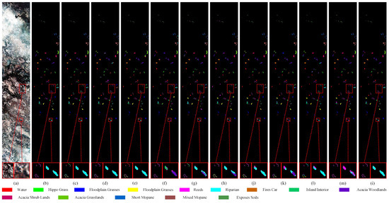
Figure 5. False-color image, ground truth, and classification maps on the Botswana dataset. (a) False-color image. (b) Ground truth. (c) DBDA (OA = 90.52%). (d) $A^2{S}^{2}K\text{-}\mathrm{Res}$ (OA = 82.57%). (e) CEGCN (OA = 86.57%). (f) FDGC (OA = 76.75%). (g) GTFN (OA = 76.82%). (h) SSFTT (OA = 80.93%). (j) GSC-ViT (OA = 90.00%). (k) DBCTNet (OA = 85.62%). (l) MambaHSI (OA = 88.20%). (m) SSLKA (OA = 87.86%). (i) MSLKACNN (OA = 92.61%).

(3) Results on Houston 2013: Table 5 presents the quantitative results achieved by different methods on the Houston 2013 dataset. From these results, it is evident that DBCTNet and GSC-ViT, which integrate convolution and Transformer, rank third and fourth, respectively, among the eleven methods. This indicates their strengths in capturing local features through the convolution and establishing long-range dependencies among pixels via the Transformer. Additionally, MSLKACNN outperforms other methods by a substantial margin in terms of OA, AA, and KAPPA, which demonstrates the superiority of our model in learning local-to-global information through asymmetric convolutions with small-to-large kernels.

Table 5. Quantitative comparison of all methods on the Houston 2013 dataset using two labeled samples per class for training.

Class	CNNs		GCNs			Transformers			Mamba	LKCNN
	DBDA	${\mathit{A}}^{\mathbf{2}}{\mathit{S}}^{\mathbf{2}}\mathit{K}$-Res	CEGCN	FDGC	GTFN	SSFTT	GSC-ViT	DBCTNet	MambaHSI	SSLKA	MSLKACNN
	RS 2020	TGRS 2021	TGRS 2021	TGRS 2022	TGRS 2023	TGRS 2022	TGRS 2024	TGRS 2024	TGRS 2024	TGRS 2024	Ours
1	87.27 ± $7.09$	59.97 ± $21.66$	79.28 ± $11.84$	57.73 ± $15.54$	68.87 ± $11.42$	82.11 ± $9.91$	89.99 ± 8.08	74.76 ± $20.92$	79.45 ± $13.09$	84.94 ± $0.63$	79.83 ± $8.95$
2	61.56 ± $12.96$	67.68 ± $20.05$	42.37 ± $18.29$	53.04 ± $12.73$	52.88 ± $15.16$	75.23 ± 5.74	59.10 ± $25.72$	62.62 ± $15.70$	70.30 ± $16.03$	65.18 ± $11.33$	67.57 ± $19.63$
3	98.32 ± $1.48$	99.70 ± $0.31$	98.57 ± $2.10$	93.81 ± $6.13$	98.22 ± $2.14$	98.71 ± $1.54$	96.51 ± $1.85$	98.83 ± $1.13$	79.33 ± $27.66$	99.97 ± 0.06	99.01 ± $1.33$
4	85.86 ± $9.73$	79.96 ± $9.86$	76.44 ± $20.10$	46.86 ± $13.77$	66.43 ± $14.02$	78.61 ± $6.80$	91.62 ± 0.73	87.58 ± $3.65$	83.95 ± $9.85$	90.86 ± $1.14$	72.74 ± $19.35$
5	90.46 ± $9.11$	87.15 ± $21.55$	92.57 ± $8.34$	84.87 ± $9.01$	78.73 ± $16.04$	99.54 ± $0.68$	87.84 ± $12.62$	93.47 ± $9.09$	95.08 ± $4.50$	99.95 ± 0.04	97.23 ± $6.95$
6	80.82 ± $3.81$	84.40 ± $3.88$	83.46 ± $6.21$	80.00 ± $6.18$	81.64 ± $6.15$	98.81 ± 0.83	82.80 ± $7.40$	82.26 ± $8.96$	75.82 ± $10.14$	83.05 ± $2.71$	87.52 ± $4.32$
7	62.89 ± $17.38$	43.35 ± $25.66$	56.32 ± $12.08$	31.79 ± $18.70$	44.68 ± $15.35$	31.32 ± $12.05$	55.83 ± $23.05$	57.26 ± $14.69$	46.99 ± $17.37$	53.66 ± $7.34$	76.51 ± 10.81
8	24.25 ± $7.25$	22.07 ± $14.74$	20.93 ± $11.68$	26.56 ± $11.11$	28.36 ± $14.38$	18.99 ± $7.36$	31.65 ± $12.83$	28.84 ± 12.53	16.69 ± $5.64$	26.64 ± $2.85$	25.46 ± $5.23$
9	59.06 ± $19.85$	40.52 ± $20.32$	57.82 ± $16.01$	36.78 ± $10.01$	57.32 ± $9.49$	29.17 ± $11.73$	62.66 ± $16.10$	64.65 ± $15.76$	60.41 ± $16.18$	49.20 ± $7.77$	71.59 ± 12.83
10	39.82 ± $9.64$	48.66 ± $20.20$	46.61 ± $13.93$	46.61 ± $9.70$	52.89 ± 12.25	33.02 ± $7.42$	42.93 ± $11.88$	45.74 ± $12.85$	35.68 ± $12.27$	33.65 ± $0.46$	37.05 ± $16.89$
11	45.86 ± $12.59$	62.44 ± $20.70$	59.80 ± $15.27$	49.89 ± $17.64$	55.27 ± $13.34$	58.58 ± $7.37$	50.34 ± $22.84$	50.86 ± $19.35$	45.11 ± $15.54$	77.89 ± 9.00	59.84 ± $10.61$
12	42.02 ± $13.47$	45.23 ± $20.61$	59.85 ± 13.04	41.54 ± $17.16$	33.60 ± $12.88$	46.04 ± $19.37$	33.35 ± $8.83$	39.21 ± $13.00$	43.97 ± $9.35$	29.57 ± $4.18$	39.32 ± $10.03$
13	86.56 ± $9.74$	86.67 ± 16.02	47.81 ± $28.90$	71.82 ± $19.52$	70.81 ± $12.57$	84.37 ± $5.71$	79.72 ± $17.72$	86.43 ± $6.38$	75.91 ± $9.98$	84.98 ± $5.88$	61.80 ± $34.31$
14	99.64 ± $0.86$	99.12 ± $1.23$	99.69 ± $0.60$	98.93 ± $1.61$	98.83 ± $0.83$	100.0 ± 0.00	93.52 ± $9.89$	95.96 ± $5.24$	99.03 ± $1.19$	99.26 ± $1.05$	100.0 ± 0.00
15	99.71 ± $0.64$	99.94 ± $0.14$	97.76 ± $1.87$	87.03 ± $13.64$	94.85 ± $6.71$	99.54 ± $1.23$	99.14 ± $1.58$	97.58 ± $4.57$	78.85 ± $14.95$	100.0 ± 0.00	99.28 ± $1.39$
OA	65.87 ± $2.52$	62.46 ± $3.97$	64.02 ± $3.08$	54.30 ± $3.85$	60.16 ± $3.09$	62.30 ± $1.78$	65.93 ± $3.44$	66.20 ± $3.30$	61.83 ± $4.46$	66.96 ± $0.68$	67.63 ± 4.55
AA	70.94 ± $2.05$	68.46 ± $3.17$	67.95 ± $3.23$	60.48 ± $3.35$	65.56 ± $2.57$	68.94 ± $1.50$	70.47 ± $3.45$	71.07 ± $3.07$	65.77 ± $4.27$	71.52 ± $0.57$	71.65 ± 4.25
KAPPA	63.26 ± $2.69$	59.55 ± $4.27$	61.08 ± $3.36$	50.70 ± $4.14$	57.07 ± $3.29$	59.31 ± $1.92$	63.24 ± $3.72$	63.56 ± $3.54$	64.00 ± $4.69$	64.35 ± $0.73$	65.08 ± 4.90

The qualitative classification maps of diverse methods are depicted in Figure 6. To aid a visual evaluation, we zoom in on the two red boxed areas in the classification maps. From these enlarged maps, we see that MSLKACNN exhibits a superior classification map in the classes of “Residential” and “Road” compared to comparison baselines.

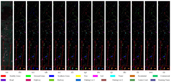
Figure 6. False-color image, ground truth, and classification maps on the Houston 2013 dataset. (a) False-color image. (b) Ground truth. (c) DBDA (OA = 65.87%). (d) $A^2{S}^{2}K\text{-}\mathrm{Res}$ (OA = 62.46%). (e) CEGCN (OA = 64.02%). (f) FDGC (OA = 54.30%). (g) GTFN (OA = 60.16%). (h) SSFTT (OA = 62.30%). (j) GSC-ViT (OA = 65.93%). (k) DBCTNet (OA = 66.20%). (l) MambaHSI (OA = 61.83%). (m) SSLKA (OA = 66.96%). (i) MSLKACNN (OA = 67.63%).

(4) Results on LongKou: Table 6 displays the numerical outcomes obtained by diverse algorithms on the LongKou dataset. Consistent with the findings from other datasets, our proposed MSLKACNN demonstrates a notable enhancement across all benchmark methods, exceeding the second place (CEGCN) by 2.20%, 6.20%, and 2.77% in terms of OA, AA, and KAPPA, respectively. This enhancement again shows the strength of our MSLKACNN.

Table 6. Quantitative comparison of all methods on the LongKou dataset using two labeled samples per class for training.

Class	CNNs		GCNs			Transformers			Mamba	LKCNN
	DBDA	${\mathit{A}}^{\mathbf{2}}{\mathit{S}}^{\mathbf{2}}\mathit{K}$-Res	CEGCN	FDGC	GTFN	SSFTT	GSC-ViT	DBCTNet	MambaHSI	SSLKA	MSLKACNN
	RS 2020	TGRS 2021	TGRS 2021	TGRS 2022	TGRS 2023	TGRS 2022	TGRS 2024	TGRS 2024	TGRS 2024	TGRS 2024	Ours
1	82.01 ± $29.90$	88.09 ± $7.21$	89.29 ± $6.92$	80.54 ± $14.33$	63.60 ± $13.24$	93.43 ± $1.83$	94.75 ± $7.52$	91.12 ± $10.46$	98.42 ± 1.78	96.86 ± $1.91$	91.20 ± $6.39$
2	62.76 ± $28.91$	77.95 ± $19.07$	76.07 ± $22.61$	68.75 ± $15.72$	67.22 ± $19.50$	57.65 ± $8.74$	67.68 ± $16.15$	66.49 ± $24.65$	62.65 ± $17.90$	87.79 ± 6.60	83.34 ± $13.64$
3	89.83 ± $7.52$	92.18 ± $8.45$	97.90 ± $2.59$	93.68 ± $7.50$	91.51 ± $6.79$	99.37 ± $0.98$	78.98 ± $11.75$	89.03 ± $8.61$	82.20 ± $10.11$	99.51 ± 0.58	95.43 ± $3.86$
4	67.47 ± $12.26$	78.42 ± $13.72$	77.49 ± $10.25$	52.49 ± $19.03$	43.16 ± $10.89$	66.08 ± $6.05$	68.50 ± $17.79$	69.98 ± $21.20$	55.07 ± $12.35$	43.49 ± $3.22$	84.57 ± 5.75
5	75.49 ± $27.95$	78.25 ± $10.41$	80.12 ± $20.94$	81.02 ± $18.16$	68.00 ± $19.48$	77.11 ± $5.14$	71.27 ± $17.80$	60.18 ± $17.11$	64.27 ± $19.96$	94.72 ± $3.74$	95.07 ± 7.29
6	82.74 ± $5.88$	60.32 ± $12.69$	91.02 ± 6.79	75.73 ± $15.26$	64.85 ± $12.74$	90.64 ± $0.48$	85.84 ± $9.05$	87.43 ± $12.83$	80.38 ± $21.05$	90.68 ± $6.75$	82.41 ± $8.68$
7	100.0 ± 0.00	87.55 ± $19.07$	98.69 ± $2.61$	85.18 ± $8.69$	84.29 ± $19.03$	97.42 ± $1.25$	99.94 ± $0.07$	99.54 ± $0.35$	97.25 ± $5.15$	99.98 ± $0.02$	93.93 ± $5.97$
8	55.59 ± $15.57$	57.24 ± $15.63$	53.25 ± $20.13$	39.45 ± $15.96$	44.08 ± $20.34$	67.87 ± $5.71$	72.60 ± 16.30	69.59 ± $21.24$	56.91 ± $19.81$	68.55 ± $2.81$	69.20 ± $16.94$
9	19.08 ± $14.12$	56.68 ± $16.46$	51.03 ± $14.14$	62.50 ± $25.96$	53.77 ± $9.77$	64.14 ± $3.39$	52.70 ± $14.50$	61.47 ± $10.56$	74.78 ± $10.66$	72.74 ± $3.17$	75.56 ± 6.57
OA	80.13 ± $6.08$	80.89 ± $7.32$	85.99 ± $4.12$	70.94 ± $5.86$	63.86 ± $6.55$	82.78 ± $1.87$	84.16 ± $5.40$	83.96 ± $6.62$	79.15 ± $4.35$	79.05 ± $1.03$	88.19 ± 3.17
AA	70.55 ± $6.96$	75.19 ± $4.83$	79.43 ± $4.10$	71.04 ± $3.95$	64.50 ± $5.65$	79.30 ± $1.42$	76.92 ± $3.78$	77.20 ± $4.55$	74.66 ± $3.21$	83.81 ± $1.03$	85.63 ± 2.57
KAPPA	74.84 ± $7.42$	75.85 ± $8.72$	82.11 ± $5.02$	64.07 ± $6.68$	55.83 ± $7.08$	77.92 ± $2.34$	79.97 ± $6.26$	79.76 ± $7.77$	66.75 ± $6.90$	74.18 ± $1.19$	84.88 ± 3.87

As illustrated in Figure 7, a visual examination indicates that the classification map of MSLKACNN is closer to the ground truth compared to other methods, especially in distinguishing the category of “Broad-Leaf Soybean”.

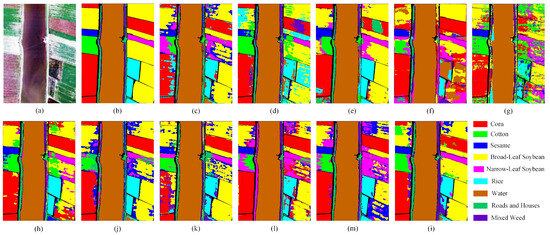
Figure 7. False-color image, ground truth, and classification maps on the LongKou dataset. (a) False-color image. (b) Ground truth. (c) DBDA (OA = 80.13%). (d) $A^2{S}^{2}K\text{-}\mathrm{Res}$ (OA = 80.89%). (e) CEGCN (OA = 85.99%). (f) FDGC (OA = 70.94%). (g) GTFN (OA = 63.86%). (h) SSFTT (OA = 82.78%). (j) GSC-ViT (OA = 84.16%). (k) DBCTNet (OA = 83.96%). (l) MambaHSI (OA = 79.15%). (m) SSLKA (OA = 79.05%). (i) MSLKACNN (OA = 88.19%).

4.4. Analysis of All Methods Under Various Numbers of Training Samples

In this section, we conduct a comparative analysis of the OA achieved by diverse methods using different numbers of training samples per class. Specifically, we utilize 2, 4, 6, 8, and 10 training samples for each dataset. A uniform number of five validation samples is maintained for all methods across all datasets. As shown in Figure 8, the OA results of most methods demonstrate an upward trend as the number of training samples increases. However, in a minority of cases, we observe that the OA results of a few competitive methods, such as GSC-ViT, decrease unexpectedly with more training samples. These anomalous results may potentially stem from the additional noise introduced by the increased training data. Conversely, the OA results of CEGCN and our proposed MSLKACNN exhibit a notable improvement with the increase in training samples. This enhancement can be credited to the noise suppression modules in their architectures. Furthermore, in most cases, our MSLKACNN consistently surpasses the comparison methods across various datasets, especially under small training sample sizes, thereby further reinforcing its robustness and superiority for HSI classification tasks.

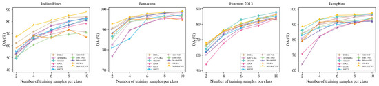
Figure 8. OA performance of various methods using different numbers of training samples per class across each dataset.

4.5. Analysis of Diverse Fusion Schemes

As described in Section 3.2, we introduce two widely used fusion schemes: column concatenation fusion (concatenate) and sum fusion (sum). In Equation (4), the number of feature maps obtained by the proposed MLKADC and MADDC is substantial. The applications of concatenate and sum for combining these feature maps have individually resulted in an increase in the number of parameters and the generation of large feature values, respectively, which may potentially lead to overfitting and gradient explosion issues. To address these challenges, we investigate the AFP fusion scheme. To evaluate our AFP, we compare the OA results achieved by AFP and the two fusion schemes. Figure 9 displays the results. From the figure, it is evident that our AFP significantly outperforms other fusion schemes. This validates the superiority of our AFP in fusing multiple feature maps.

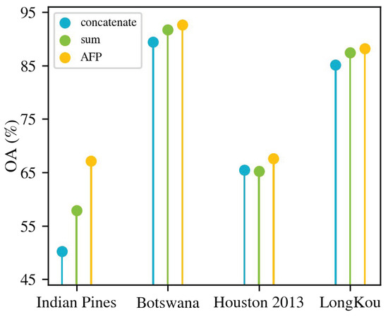
Figure 9. OA results of diverse fusion schemes on each dataset.

4.6. Analysis of Computational Complexity

Table 7 provides an extensive evaluation in terms of the training time, testing time, parameters, and FLOPS across all methods. The analysis yields the following insights: (1) SSFTT demonstrates faster training speeds compared to other baseline methods, which can be attributed to its use of a limited number of convolutional layers. (2) CEGCN and MambaHSI operate on the whole HSI as input instead of using small HSI cubes, leading to quicker prediction speeds than most other methods. (3) Like CEGCN and MambaHSI, the proposed MSLKACNN also processes the entire HSI as input, achieving the fastest prediction time across all datasets. (4) LKVHAN outperforms most methods in terms of parameters, due to its replacement of square kernels with vertical and horizontal kernels. (5) Since CEGCN, MambaHSI, and MSLKACNN take the entire HSI as input, they require significantly more FLOPS compared to other approaches that use small HSI cubes. Additionally, MSLKACNN significantly outperforms other methods in terms of the classification results. These findings highlight the benefits of incorporating small-to-large kernel asymmetric convolutions in MSLKACNN for industrial applications.

Table 7. Analysis of different methods in terms of training time, testing time, parameters, and FLOPS on the Indian Pines, Botswana, Houston 2013, and LongKou datasets. CEGCN, MambaHSI, and our proposed MSLKACNN process the entire HSI as input, while other models utilize small HSI cubes. The FLOPS results for these other models are calculated with a batch size of 1. s, ms, K, and G, denote second, millisecond, kilo, and giga, respectively.

Dataset	Metrics	CNNs		GCNs			Transformers			Mamba	LKCNN
		DBDA	${\mathit{A}}^{\mathbf{2}}{\mathit{S}}^{\mathbf{2}}\mathit{K}$-Res	CEGCN	FDGC	GTFN	SSFTT	GSC-ViT	DBCTNet	MambaHSI	SSLKA	MSLKACNN
		RS 2020	TGRS 2021	TGRS 2021	TGRS 2022	TGRS 2023	TGRS 2022	TGRS 2024	TGRS 2024	TGRS 2024	TGRS 2024	Ours
Indian Pines	Train time (s)	6.80	2.51	14.86	4.60	15.56	1.96	9.06	24.24	32.33	9.40	1.28
	Test time (s)	6.27	2.03	9.95 ms	1.05	6.28	0.53	1.88	1.14	6.52 ms	0.95	1.77 ms
	Parameters (K)	382.3	370.8	166.4	2445.4	169.3	148.5	563.7	30.3	44.3	136.9	33.9
	FLOPS (G)	0.108	0.104	1.610	0.015	0.012	0.011	0.021	0.012	0.563	0.007	0.716
Botswana	Train time (s)	4.70	2.34	1418.43	3.28	15.32	1.82	7.78	15.30	459.14	8.89	20.03
	Test time (s)	1.29	0.56	0.94	0.31	1.97	0.14	30.60	0.27	27.49 ms	0.29	13.28 ms
	Parameters (K)	280.0	80.5	159.0	2313.4	169.2	148.4	103.1	22.5	37.0	134.1	30.2
	FLOPS (G)	0.098	0.005	26.131	0.015	0.012	0.011	0.007	0.009	7.457	0.007	11.487
Houston 2013	Train time (s)	4.57	2.60	709.95	3.46	15.47	1.83	9.01	22.82	892.93	8.60	21.03
	Test time (s)	5.96	2.67	2.53	1.31	9.71	0.73	64.40	1.08	240.26 ms	1.35	16.67 ms
	Parameters (K)	280.1	83.6	159.1	2379.4	169.2	148.4	88.8	22.2	37.0	134.1	30.2
	FLOPS (G)	0.077	0.007	45.964	0.015	0.012	0.011	0.006	0.009	13.039	0.007	20.211
LongKou	Train time (s)	4.05	2.40	459.79	2.85	14.81	1.35	7.87	23.15	272.31	6.85	10.36
	Test time (s)	155.81	35.92	0.35	17.95	127.29	9.08	21.30	32.48	22.15 ms	19.58	2.41 ms
	Parameters (K)	509.2	74.0	174.6	1983.3	168.8	148.0	173.1	40.3	52.4	140.0	37.9
	FLOPS (G)	0.146	0.003	18.700	0.014	0.012	0.011	0.010	0.017	7.852	0.007	8.378

4.7. Ablation Study

The proposed MSLKACNN comprises three primary components, the SFEM, the MLKADC, and the MADDC, as well as two critical hyperparameters, the large kernel size in MLKADC and the large kernel size in MADDC. In this section, we perform ablation studies to assess the individual contributions and impact of the three components and the two hyperparameters.

(1) Contributions of Each Component: To assess the individual contributions of these components, we perform a quantitative analysis by selectively removing one of the three components. The results are summarized in Table 8. To ensure consistency between the number of bands in the original HSI and the number of filters in the convolutional layers, we retain one of the $1\times 1$ convolution blocks from the SFEM component after its removal. From the table, we observe that the MSLKACNN model without the MLKADC component exhibits suboptimal performance in comparison to other models across most datasets. This indicates that the component plays a more significant role compared to the other components. Moreover, our MSLKACNN consistently surpasses the performance of its modified versions on all datasets. These findings reinforce the effectiveness of the integrated components.

Table 8. Classification results of each component in MSLKACNN.

SFEM	MLKADC	MADDC	Indian Pines			Botswana			Houston 2013			LongKou
			OA	AA	KAPPA	OA	AA	KAPPA	OA	AA	KAPPA	OA	AA	KAPPA
✕	√	√	59.06	76.25	54.57	90.20	90.56	89.38	62.79	67.28	59.91	87.45	83.99	84.00
√	✕	√	50.29	63.78	44.96	86.31	87.42	85.18	64.89	69.19	62.11	79.09	80.43	73.83
√	√	✕	64.22	79.43	60.35	90.39	91.18	89.59	64.47	69.65	61.73	82.15	81.19	77.61
√	√	√	67.14	80.15	63.30	92.61	92.89	91.99	67.63	71.65	65.08	88.19	85.63	84.88

(2) Analysis of Various Large Kernel Sizes in MLKADC: To verify the effect of different large kernel sizes in MLKADC, we conduct a comparative analysis of OA using varying large kernel sizes across four benchmark datasets: Indian Pines, Botswana, Houston 2013, and LongKou. The results are visually depicted in Figure 10. The figure illustrates a significant trend: the OA tends to increase with the enlargement of kernel sizes in most cases, reaching its peak at kernel sizes of $1\times 17$ and $17\times 1$. Nevertheless, a further increase in kernel sizes leads to a decline in OA. This discovery is vital for determining the optimal large kernel sizes for MLKADC.

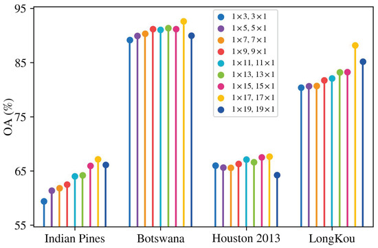
Figure 10. OA results of various large kernel sizes in MLKADC on each dataset.

(3) Analysis of Different Kernel Sizes in MADDC: To evaluate the influence of various kernel sizes in MADDC, we compare the OA results achieved by diverse kernel sizes on the Indian Pines, Botswana, Houston 2013, and LongKou datasets. These results are illustrated in Figure 11. We observe that the MSLKACNN model equipped with the kernel sizes of $1\times 5$ and $5\times 1$ exhibits superior performance compared to its variant models utilizing alternative kernel sizes, thereby determining the optimal kernel sizes for MADDC.

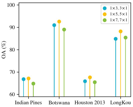
Figure 11. OA results of different kernel sizes in MADDC on each dataset.

5. Conclusions

In this paper, we propose MSLKACNN, a novel multi-scale large kernel asymmetric CNN architecture for HSI classification. The key breakthrough of our MSLKACNN lies in successfully scaling up convolutional kernels to $1\times 17$ and $17\times 1$ sizes while maintaining computational efficiency. The core innovation of the proposed MSLKACNN is the MSLKAC component, which combines asymmetric depthwise convolutions with small to large kernels and asymmetric dilated depthwise convolutions, effectively extracting both local and global features. Our MSLKACNN achieves the best performance in terms of OA, AA, and KAPPA, compared to baseline methods, demonstrating its effectiveness and superiority. In the future, we will explore replacing a large kernel asymmetric convolution with multiple small kernel asymmetric convolutions to maintain a large receptive field while reducing the number of parameters and computational costs.

6. Further Discussion

As shown in Table 3, Table 4, Table 5 and Table 6, the proposed MSLKACNN demonstrates superior performance compared to those of five major categories of deep learning approaches: (1) CNNs, (2) GCNs, (3) Transformers, (4) Mamba, and (5) LKCNN. From these results, we observe that the LKCNN method SSLKA exhibits significantly lower classification performance than most benchmark methods on the high-density dataset (LongKou), while outperforming most comparative methods on the remaining datasets (Indian Pines, Botswana, and Houston 2013). This implies that SSLKA may be unsuitable for processing dense HSI data. Notably, compared to the most related method, SSLKA, the proposed MSLKACNN shows significant performance improvement across all datasets, with OA improvements of 9.18%, 4.75%, 0.67%, and 9.14% on the Indian Pines, Botswana, Houston 2013, and LongKou datasets, respectively. These performance gains can be attributed to the enhanced capabilities of MSLKACNN to extract and integrate both local and global features through asymmetric convolutions with small-to-large kernels. In addition, as shown in Table 7, our MSLKACNN outperforms SSLKA by a large margin in terms of parameters and testing time, demonstrating the advantages of replacing square kernels with vertical and horizontal kernels in MSLKACNN.

Although the proposed MSLKACNN demonstrates significant advantages in classification performance, inference speed, and parameters, the use of entire HSI rather than its small cubes as input leads to higher computational complexity, posing challenges when dealing with extremely large-scale datasets. Furthermore, while our parallel asymmetric convolutions with small-to-large kernels effectively capture local-to-global features, the absence of an attention mechanism may limit the model’s ability to focus on critical spatial features, which could affect discriminative feature learning in complex scenarios.

References

- Yuan, J.; Wang, S.; Wu, C.; Xu, Y. Fine-grained classification of urban functional zones and landscape pattern analysis using hyperspectral satellite imagery: A case study of Wuhan. IEEE J. Sel. Top. Appl. Earth Observ. Remote Sens. 2022, 15, 3972–3991. [Google Scholar] [CrossRef]
- Gevaert, C.M.; Suomalainen, J.; Tang, J.; Kooistra, L. Generation of Spectral–Temporal Response Surfaces by Combining Multispectral Satellite and Hyperspectral UAV Imagery for Precision Agriculture Applications. IEEE J. Sel. Topics Appl. Earth Observ. Remote Sens. 2015, 8, 3140–3146. [Google Scholar] [CrossRef]
- Murphy, R.J.; Schneider, S.; Monteiro, S.T. Consistency of Measurements of Wavelength Position From Hyperspectral Imagery: Use of the Ferric Iron Crystal Field Absorption at ∼900 nm as an Indicator of Mineralogy. IEEE Trans. Geosci. Remote Sens. 2014, 52, 2843–2857. [Google Scholar] [CrossRef]
- Vibhute, A.D.; Kale, K.V.; Dhumal, R.K.; Mehrotra, S.C. Hyperspectral imaging data atmospheric correction challenges and solutions using QUAC and FLAASH algorithms. In Proceedings of the International Conference on Man and Machine Interfacing (MAMI), Bhubaneswar, India, 17–19 December 2015; pp. 1–6. [Google Scholar]
- Ryan, J.P.; Davis, C.O.; Tufillaro, N.B.; Kudela, R.M.; Gao, B.C. Application of the hyperspectral imager for the coastal ocean to phytoplankton ecology studies in Monterey Bay, CA, USA. Remote Sens. 2014, 6, 1007–1025. [Google Scholar] [CrossRef]
- Li, Z.; Xiong, F.; Zhou, J.; Lu, J.; Qian, Y. Learning a Deep Ensemble Network with Band Importance for Hyperspectral Object Tracking. IEEE Trans. Image Process. 2023, 32, 2901–2914. [Google Scholar] [CrossRef]
- Zhang, B.; Li, S.; Jia, X.; Gao, L.; Peng, M. Adaptive Markov Random Field Approach for Classification of Hyperspectral Imagery. IEEE Geosci. Remote Sens. Lett. 2011, 8, 973–977. [Google Scholar] [CrossRef]
- Li, R.; Zheng, S.; Duan, C.; Yang, Y.; Wang, X. Classification of hyperspectral image based on double–branch dual–attention mechanism network. Remote Sens. 2020, 12, 582. [Google Scholar] [CrossRef]
- Liu, Q.; Xiao, L.; Yang, J.; Wei, Z. CNN-enhanced graph convolutional network with pixel-and superpixel-level feature fusion for hyperspectral image classification. IEEE Trans. Geosci. Remote Sens. 2021, 59, 8657–8671. [Google Scholar] [CrossRef]
- Sun, L.; Zhao, G.; Zheng, Y.; Wu, Z. Spectral–spatial feature tokenization transformer for hyperspectral image classification. IEEE Trans. Geosci. Remote Sens. 2022, 60, 1–14. [Google Scholar] [CrossRef]
- Yang, X.; Ye, Y.; Li, X.; Lau, R.Y.; Zhang, X.; Huang, X. Hyperspectral image classification with deep learning models. IEEE Trans. Geosci. Remote Sens. 2018, 56, 5408–5423. [Google Scholar] [CrossRef]
- Chen, Y.; Lin, Z.; Zhao, X.; Wang, G.; Gu, Y. Deep learning-based classification of hyperspectral data. IEEE J. Sel. Topics Appl. Earth Observ. Remote Sens. 2014, 7, 2094–2107. [Google Scholar] [CrossRef]
- Mou, L.; Ghamisi, P.; Zhu, X.X. Deep recurrent neural networks for hyperspectral image classification. IEEE Trans. Geosci. Remote Sens. 2017, 55, 3639–3655. [Google Scholar] [CrossRef]
- Li, Y.; Zhang, H.; Shen, Q. Spectral–spatial classification of hyperspectral imagery with 3D convolutional neural network. Remote Sens. 2017, 9, 67. [Google Scholar] [CrossRef]
- Zhang, M.; Li, W.; Du, Q. Diverse region–based CNN for hyperspectral image classification. IEEE Trans. Image Process. 2018, 27, 2623–2634. [Google Scholar] [CrossRef]
- Paoletti, M.E.; Haut, J.M.; Fernandez-Beltran, R.; Plaza, J.; Plaza, A.; Li, J.; Pla, F. Capsule networks for hyperspectral image classification. IEEE Trans. Image Process. 2019, 57, 2145–2160. [Google Scholar] [CrossRef]
- Qin, A.; Shang, Z.; Tian, J.; Wang, Y.; Zhang, T.; Tang, Y.Y. Spectral–spatial graph convolutional networks for semisupervised hyperspectral image classification. IEEE Geosci. Remote Sens. Lett. 2019, 16, 241–245. [Google Scholar] [CrossRef]
- Bai, J.; Ding, B.; Xiao, Z.; Jiao, L.; Chen, H.; Regan, A.C. Hyperspectral image classification based on deep attention graph convolutional network. IEEE Trans. Geosci. Remote Sens. 2021, 60, 1–16. [Google Scholar] [CrossRef]
- Hong, D.; Han, Z.; Yao, J.; Gao, L.; Zhang, B.; Plaza, A.; Chanussot, J. SpectralFormer: Rethinking hyperspectral image classification with transformers. IEEE Trans. Geosci. Remote Sens. 2021, 60, 1–15. [Google Scholar] [CrossRef]
- Li, Y.; Luo, Y.; Zhang, L.; Wang, Z.; Du, B. MambaHSI: Spatial-Spectral Mamba for Hyperspectral Image Classification. IEEE Trans. Geosci. Remote Sens. 2024, 62, 1–16. [Google Scholar] [CrossRef]
- Wang, W.; Dou, S.; Jiang, Z.; Sun, L. A fast dense spectral–spatial convolution network framework for hyperspectral images classification. Remote Sens. 2018, 10, 1068. [Google Scholar] [CrossRef]
- Li, Z.; Huang, L.; He, J. A multiscale deep middle-level feature fusion network for hyperspectral classification. Remote Sens. 2019, 11, 695. [Google Scholar] [CrossRef]
- Wang, X.; Tan, K.; Du, P.; Pan, C.; Ding, J. A unified multiscale learning framework for hyperspectral image classification. IEEE Trans. Geosci. Remote Sens. 2022, 60, 1–19. [Google Scholar] [CrossRef]
- Roy, S.K.; Manna, S.; Song, T.; Bruzzone, L. Attention-based adaptive spectral–spatial kernel ResNet for hyperspectral image classification. IEEE Trans. Geosci. Remote Sens. 2021, 59, 7831–7843. [Google Scholar] [CrossRef]
- Li, M.; Liu, Y.; Xue, G.; Huang, Y.; Yang, G. Exploring the relationship between center and neighborhoods: Central vector oriented self-similarity network for hyperspectral image classification. IEEE Trans. Circ. Syst. Vid. 2023, 33, 1979–1993. [Google Scholar] [CrossRef]
- Kipf, T.N.; Welling, M. Semi–supervised classification with graph convolutional networks. In Proceedings of the International Conference on Learning Representations, (ICLR), Toulon, France, 24–26 April 2017; pp. 1–14. [Google Scholar]
- Liu, Q.; Dong, Y.; Zhang, Y.; Luo, H. A Fast Dynamic Graph Convolutional Network and CNN Parallel Network for Hyperspectral Image Classification. IEEE Trans. Geosci. Remote Sens. 2022, 60, 1–15. [Google Scholar] [CrossRef]
- Zhou, H.; Luo, F.; Zhuang, H.; Weng, Z.; Gong, X.; Lin, Z. Attention Multihop Graph and Multiscale Convolutional Fusion Network for Hyperspectral Image Classification. IEEE Trans. Geosci. Remote Sens. 2023, 61, 1–14. [Google Scholar] [CrossRef]
- Liu, X.; Ng, A.H.M.; Ge, L.; Lei, F.; Liao, X. Multibranch Fusion: A Multibranch Attention Framework by Combining Graph Convolutional Network and CNN for Hyperspectral Image Classification. IEEE Trans. Geosci. Remote Sens. 2024, 62, 1–17. [Google Scholar] [CrossRef]
- Dosovitskiy, A.; Beyer, L.; Kolesnikov, A.; Weissenborn, D.; Zhai, X.; Unterthiner, T.; Dehghani, M.; Minderer, M.; Heigold, G.; Gelly, S.; et al. An image is worth 16x16 words: Transformers for image recognition at scale. arXiv 2020, arXiv:2010.11929. [Google Scholar]
- Yang, A.; Li, M.; Ding, Y.; Hong, D.; Lv, Y.; He, Y. GTFN: GCN and Transformer Fusion Network with Spatial-Spectral Features for Hyperspectral Image Classification. IEEE Trans. Geosci. Remote Sens. 2023, 61, 1–15. [Google Scholar] [CrossRef]
- Zhao, Z.; Xu, X.; Li, S.; Plaza, A. Hyperspectral Image Classification Using Groupwise Separable Convolutional Vision Transformer Network. IEEE Trans. Geosci. Remote Sens. 2024, 62. [Google Scholar] [CrossRef]
- Xu, R.; Dong, X.M.; Li, W.; Peng, J.; Sun, W.; Xu, Y. DBCTNet: Double branch convolution-transformer network for hyperspectral image classification. IEEE Trans. Geosci. Remote Sens. 2024, 62, 1–15. [Google Scholar] [CrossRef]
- Yao, J.; Hong, D.; Li, C.; Chanussot, J. Spectralmamba: Efficient mamba for hyperspectral image classification. arXiv 2024, arXiv:2404.08489. [Google Scholar]
- Gu, A.; Dao, T. Mamba: Linear-time sequence modeling with selective state spaces. arXiv 2023, arXiv:2312.00752. [Google Scholar]
- Ding, X.; Zhang, X.; Han, J.; Ding, G. Scaling up your kernels to 31x31: Revisiting large kernel design in cnns. In Proceedings of the IEEE/CVF Conference on Computer Vision and Pattern Recognition (CVPR), New Orleans, LA, USA, 18–24 June 2022; pp. 11963–11975. [Google Scholar]
- Liu, S.; Chen, T.; Chen, X.; Chen, X.; Xiao, Q.; Wu, B.; Kärkkäinen, T.; Pechenizkiy, M.; Mocanu, D.; Wang, Z. More convnets in the 2020s: Scaling up kernels beyond 51x51 using sparsity. arXiv 2022, arXiv:2207.03620. [Google Scholar]
- Ding, X.; Zhang, Y.; Ge, Y.; Zhao, S.; Song, L.; Yue, X.; Shan, Y. UniRepLKNet: A Universal Perception Large-Kernel ConvNet for Audio Video Point Cloud Time-Series and Image Recognition. In Proceedings of the IEEE/CVF Conference on Computer Vision and Pattern Recognition (CVPR), Seattle, WA, USA, 16–22 June 2024; pp. 5513–5524. [Google Scholar]
- Zhong, C.; Gong, N.; Zhang, Z.; Jiang, Y.; Zhang, K. LiteCCLKNet: A lightweight criss-cross large kernel convolutional neural network for hyperspectral image classification. IET Comput. Vis. 2023, 17, 763–776. [Google Scholar] [CrossRef]
- Sun, G.; Pan, Z.; Zhang, A.; Jia, X.; Ren, J.; Fu, H.; Yan, K. Large kernel spectral and spatial attention networks for hyperspectral image classification. IEEE Trans. Geosci. Remote Sens. 2023, 61, 1–15. [Google Scholar] [CrossRef]
- Wu, C.; Tong, L.; Zhou, J.; Xiao, C. Spectral-Spatial Large Kernel Attention Network for Hyperspectral Image Classification. IEEE Trans. Geosci. Remote Sens. 2024, 42. [Google Scholar] [CrossRef]
- Howard, A.G.; Zhu, M.; Chen, B.; Kalenichenko, D.; Wang, W.; Weyand, T.; Andreetto, M.; Adam, H. Mobilenets: Efficient convolutional neural networks for mobile vision applications. In Proceedings of the IEEE IEEE Conference on Computer Vision and Pattern Recognition (CVPR), Honolulu, HI, USA, 21–26 July 2017; pp. 1–9. [Google Scholar]
- Yu, F.; Koltun, V. Multi–scale context aggregation by dilated convolutions. In Proceedings of the International Conference on Learning Representations (ICLR), San Juan, Puerto Rico, 2–4 May 2016. [Google Scholar]
- Plaza, A.; Martinez, P.; Perez, R.; Plaza, J. A new approach to mixed pixel classification of hyperspectral imagery based on extended morphological profiles. Pattern Recogn. 2004, 37, 1097–1116. [Google Scholar] [CrossRef]
- Hu, W.; Huang, Y.; Wei, L.; Zhang, F.; Li, H. Deep convolutional neural networks for hyperspectral image classification. J. Sens. 2015, 2015, 1–12. [Google Scholar] [CrossRef]
- Zhao, W.; Du, S. Spectral–spatial feature extraction for hyperspectral image classification: A dimension reduction and deep learning approach. IEEE Trans. Geosci. Remote Sens. 2016, 54, 4544–4554. [Google Scholar] [CrossRef]
- Yang, J.; Zhao, Y.Q.; Chan, J.C.W. Learning and transferring deep joint spectral–spatial features for hyperspectral classification. IEEE Trans. Geosci. Remote Sens. 2017, 55, 4729–4742. [Google Scholar] [CrossRef]
- Chen, C.; Zhang, J.J.; Zheng, C.H.; Yan, Q.; Xun, L.N. Classification of hyperspectral data using a multi-channel convolutional neural network. In Proceedings of the International Conference Intelligent Computing (ICIC), Wuhan, China, 15–18 August 2018; pp. 81–92. [Google Scholar]
- Zhong, Z.; Li, J.; Luo, Z.; Chapman, M. Spectral–spatial residual network for hyperspectral image classification: A 3-D deep learning framework. IEEE Trans. Geosci. Remote Sens. 2018, 56, 847–858. [Google Scholar] [CrossRef]
- He, K.; Zhang, X.; Ren, S.; Sun, J. Deep residual learning for image recognition. In Proceedings of the IEEE Conference on Computer Vision and Pattern Recognition (CVPR), Las Vegas, NV, USA, 27–30 June 2016; pp. 770–778. [Google Scholar]
- Huang, G.; Liu, Z.; Van Der Maaten, L.; Weinberger, K.Q. Densely connected convolutional networks. In Proceedings of the IEEE Conference on Computer Vision and Pattern Recognition (CVPR), Honolulu, HI, USA, 21–26 July 2017; pp. 4700–4708. [Google Scholar]
- Chen, Y.; Jiang, H.; Li, C.; Jia, X.; Ghamisi, P. Deep feature extraction and classification of hyperspectral images based on convolutional neural networks. IEEE Trans. Geosci. Remote Sens. 2016, 54, 6232–6251. [Google Scholar] [CrossRef]
- Li, Y.; Xie, W.; Li, H. Hyperspectral image reconstruction by deep convolutional neural network for classification. Pattern Recogn. 2017, 63, 371–383. [Google Scholar] [CrossRef]
- Gong, Z.; Zhong, P.; Yu, Y.; Hu, W.; Li, S. A CNN with multiscale convolution and diversified metric for hyperspectral image classification. IEEE Trans. Geosci. Remote Sens. 2019, 57, 3599–3618. [Google Scholar] [CrossRef]
- Ding, Y.; Zhang, Z.; Zhao, X.; Hong, D.; Li, W.; Cai, W.; Zhan, Y. AF2GNN: Graph convolution with adaptive filters and aggregator fusion for hyperspectral image classification. Inf. Sci. 2022, 602, 201–219. [Google Scholar] [CrossRef]
- Wang, D.; Du, B.; Zhang, L. Spectral-spatial global graph reasoning for hyperspectral image classification. IEEE Trans. Neur. Net. Lear. 2023, 1–14. [Google Scholar] [CrossRef]
- Dong, Y.; Liu, Q.; Du, B.; Zhang, L. Weighted feature fusion of convolutional neural network and graph attention network for hyperspectral image classification. IEEE Trans. Image Process. 2022, 31, 1559–1572. [Google Scholar] [CrossRef]
- He, J.; Zhao, L.; Yang, H.; Zhang, M.; Li, W. HSI-BERT: Hyperspectral Image Classification Using the Bidirectional Encoder Representation From Transformers. IEEE Trans. Geosci. Remote Sens. 2020, 58, 165–178. [Google Scholar] [CrossRef]
- Vaswani, A.; Shazeer, N.; Parmar, N.; Uszkoreit, J.; Jones, L.; Gomez, A.N.; Kaiser, Ł.; Polosukhin, I. Attention is all you need. Proc. Adv. Neural Inf. Process. Syst. (NeurIPS) 2017, 30, 1–11. [Google Scholar]
- Zhao, F.; Zhang, J.; Meng, Z.; Liu, H.; Chang, Z.; Fan, J. Multiple vision architectures-based hybrid network for hyperspectral image classification. Expert Syst. Appl. 2023, 234, 121032. [Google Scholar] [CrossRef]
- Zhou, W.; Kamata, S.I.; Wang, H.; Wong, M.S.; Hou, H.C. Mamba-in-Mamba: Centralized Mamba-Cross-Scan in Tokenized Mamba Model for Hyperspectral Image Classification. arXiv 2024, arXiv:2405.12003. [Google Scholar] [CrossRef]
- Gao, H.; Yang, Y.; Li, C.; Gao, L.; Zhang, B. Multiscale residual network with mixed depthwise convolution for hyperspectral image classification. IEEE Trans. Geosci. Remote Sens. 2021, 59, 3396–3408. [Google Scholar] [CrossRef]
- Zhao, F.; Zhang, J.; Meng, Z.; Liu, H. Densely connected pyramidal dilated convolutional network for hyperspectral image classification. Remote Sens. 2021, 13, 3396. [Google Scholar] [CrossRef]
- Debes, C.; Merentitis, A.; Heremans, R.; Hahn, J.; Frangiadakis, N.; van Kasteren, T.; Liao, W.; Bellens, R.; Pižurica, A.; Gautama, S.; et al. Hyperspectral and LiDAR data fusion: Outcome of the 2013 GRSS data fusion contest. IEEE J. Sel. Top. Appl. Earth Obs. Remote. Sens. 2014, 7, 2405–2418. [Google Scholar] [CrossRef]
- Zhong, Y.; Hu, X.; Luo, C.; Wang, X.; Zhao, J.; Zhang, L. WHU-Hi: UAV-borne hyperspectral with high spatial resolution (H2) benchmark datasets and classifier for precise crop identification based on deep convolutional neural network with CRF. Remote Sens. Environ. 2020, 250, 112012. [Google Scholar] [CrossRef]
Disclaimer/Publisher’s Note: The statements, opinions and data contained in all publications are solely those of the individual author(s) and contributor(s) and not of MDPI and/or the editor(s). MDPI and/or the editor(s) disclaim responsibility for any injury to people or property resulting from any ideas, methods, instructions or products referred to in the content. |
© 2025 by the authors. Licensee MDPI, Basel, Switzerland. This article is an open access article distributed under the terms and conditions of the Creative Commons Attribution (CC BY) license (https://creativecommons.org/licenses/by/4.0/).