Abstract
Spaceborne synthetic aperture radar (SAR) has been proven capable of observing the directional ocean wave spectrum across the global ocean. Most of the efforts focus on the integrated wave parameters to characterize the imaged ocean wave properties. The newly proposed spectrum-based radar parameter mean cross-spectrum (MACS) is investigated using SAR image spectral properties of range-traveling waves at a wavelength of 20 m, based on Sentinel-1 wave mode acquisition of high spatial resolution (5 m). The magnitude of MACS is documented relative to environmental conditions (wind speed and direction) in terms of its variation for two polarizations at two incidence angles. This parameter exhibits distinct upwind–downwind asymmetry and polarization ratio at two incidence angles (23.8° and 36.8°). In addition, by comparing the SAR measurements with simulated MACS, we derive an improved real aperture radar modulation transfer function. Results obtained in this study shall help obtain a more accurate ocean wave spectrum based on the improved RAR modulations.
1. Introduction
Ocean waves are commonly present on the sea surface, and the formulation of a two-dimensional ocean wave spectrum is expressed as functions of wind forcing, wind fetch, and duration and presence of long ocean swell [1,2]. Spaceborne synthetic aperture radar (SAR) has been demonstrated to be effective in capturing the fine-scale variations of sea surface roughness associated with a broad range of geophysical phenomena [3]. Its applications include the observation of ocean surface waves [4], upper oceanic currents [5], and internal waves [6], among others. SAR also has proven efficacy in detecting features such as marginal sea ice, as evidenced in previous studies [7,8,9]. Among these applications, ocean wave monitoring relies on the retrieval of a two-dimensional ocean wave spectrum from SAR measurements [4,10,11]. While the basic principle of nonlinear SAR mapping transformations is well understood, the inversion scheme of ocean wave spectra is complex given its nonlinearity. With increasing SAR spatial resolution, SAR ocean wave observations have brought new opportunities. The previous SAR systems with spatial spacing around 30 m have posed a limitation in the observation of ocean waves, confining investigations largely to ocean swell with wavelengths longer than 100 m [12,13,14,15,16]. However, the advent of the Sentinel-1 wave mode, with a significantly finer spatial resolution of approximately 5 m, makes it possible to study the wave spectra of wind-driven waves. The high spatial resolution of Sentinel-1 wave mode not only expands the scope of ocean wave studies but also enables a finer exploration of the complex interactions between wind, waves, and the underlying ocean dynamics.
SAR measurements of ocean wave spectra can be roughly divided into two primary methodologies: the Max Planck Institute scheme detailed in [4] and the quasi-linear inversion scheme [17]. The Max Planck Institute algorithm employs an initial estimate of the directional wave spectrum obtained from external sources and iteratively refines it by minimizing a cost function. The cost function is commonly taken as the integral of the SAR-measured image spectrum and the predicted image spectrum based on the input ocean wave spectrum. The optimal wave spectrum solution is finally yielded through minimization of the cost function [18]. It should be noted that this scheme preserves the nonlinear aspect of SAR imaging transformation, enhancing to some extent the retrieval accuracy of a directional wave spectrum. However, its limitation lies in its dependence on a priori wave spectra from either numerical outputs or theoretical estimates [9]. On the other hand, the quasi-linear inversion scheme eliminates the prerequisite for an initial guess of the wave spectrum by removing the nonlinear component, facilitating a more straightforward inversion process [19]. This algorithm has been used as an operational scheme of ocean wave spectrum inversion since the wave mode of advanced SAR ASAR and subsequently of Sentinel-1. A common aspect of these approaches lies in addressing the nonlinear distortions associated with the azimuth cutoff as well as the modulation transfer function (MTF) of the input real aperture radar (RAR). To be specific, the RAR mapping of ocean waves involves two modulation processes: tilt and hydrodynamic modulations. The RAR MTF constitutes the mathematical formulation linking the ocean wave spectrum to the modulation signal measured by a real aperture radar, in the case of a SAR sensor, to be further modulated by the velocity bunching process [4]. Numerous investigations have delved into evaluating RAR modulation as exemplified by [20]. Additionally, studies have explored the influence of dual-polarization effects on RAR, as discussed by [13]. The complexity of these inversion processes underscores the challenges in accurately characterizing ocean wave spectra through SAR measurements, laying the groundwork for continuous research and refinement in these methodologies.
Ocean wave spectrum has been known as an effective way to describe the wave energy distribution over a broad range of wave frequency (wavenumber) and directions [1]. Most of the investigations also take advantage of integrated wave parameters for wave characteristics study [2,21], while a few utilize the sub-integrated wave parameters [22]. As an extended effort, the assessment of SAR wave observations has been carried out through a recently proposed SAR image cross-spectrum-based parameter, termed mean cross-spectra (MACS) [23]. Unlike traditional approaches requiring computationally demanding inversion of the entire ocean wave spectrum, MACS offers a novel methodology based on SAR image cross-spectra. The definition of MACS involves a distinctive process targeting intermediate ocean waves traveling in the range direction. This definition enables the precise identification and characterization of ocean waves of interest, bypassing the need for resource-intensive inversions. In specifics, the MACS parameter is derived through a dual-filtering process that applies criteria along both the range and azimuthal directions. In the azimuthal direction, only wavelengths exceeding 600 m are considered to minimize the impact of nonlinear velocity bunching in SAR imaging. Meanwhile, in the range direction, wavelengths between 15 m and 20 m are selected, with the lower limit set at approximately three times the nominal spatial resolution of Sentinel-1. This selective filtering is implemented to minimize nonlinear distortions induced by velocity bunching, thereby enhancing the interpretability of the resulting MACS parameter. Effectively, the derived MACS can be interpreted as the wave spectrum of range-traveling intermediate waves, weighted by the RAR MTF. This innovative approach introduces MACS as an additional dimension to traditional radar backscattering, providing a valuable tool for investigating the characteristics of ocean waves under diverse radar configurations and environmental conditions. The MACS parameter not only simplifies the computational burden associated with wave spectrum inversion but also offers insights into the dynamics of ocean waves, opening avenues for advanced studies in radar remote sensing of marine environments.
In this study, we will look into the statistical behavior of MACS magnitude utilizing dual-polarization SAR data obtained from Sentinel-1A (VV polarization) and Sentinel-1B (HH polarization). Our investigation focuses on two primary aspects. Firstly, we document the statistical properties of MACS, including aspects such as the azimuthal modulation versus the relative wind direction, the upwind-to-downwind asymmetry, and the upwind-to-crosswind asymmetry. This innovative parameter is tailored to minimize the influence of nonlinear distortions induced by the velocity bunching of long ocean waves. Another key advantage is that it holds significant potential to enhance our understanding of refined RAR MTF values, which provides an avenue for advancing our comprehension of SAR imaging principles of ocean waves. Furthermore, we derive an improved RAR modulation through a comparative analysis between the simulated MACS based on the quasi-nonlinear transformations and the obtained SAR measurements at both polarizations and two incidence angles. The remainder of this paper is organized as follows. Section 2 provides an overview of Sentinel-1 acquisitions and the collocated dataset of wind vectors along with the definitions of MACS. Section 3 conducts an in-depth analysis of the statistical characteristics of MACS, including the noise removal, and the azimuthal modulations. Subsequently, Section 4 details the procedure for deriving RAR modulation based on the comparison of MACS between simulations and actual measurements. Conclusions are finally presented in Section 5.
2. Dataset and MACS
2.1. Sentinel-1 Wave Mode
The Sentinel satellites are missions of the European Space Agency centering on Earth observations, including microwave radars, optical sensors, and so on. Among these, the first of the series, the Sentinel-1 satellite constellation, is composed of two identical instruments: Sentinel-1A and Sentinel-1B. This satellite is designed to serve a wide range of applications across multiple domains, such as sea and land monitoring, rapid response to environmental crises, and economic endeavors. The rich acquisitions collected by Sentinel-1 across the globe provide a database for the needs of these diverse applications. To fulfill these goals, Sentinel-1 operates in four imaging modes, including interferometric wide swath, extra wide swath, stripmap, and wave (WV). Interferometric wide mode offers wide swath coverage with a spatial resolution of around 5 m by 20 m and is primarily used for large-scale monitoring and mapping applications. Similar to the interferometric wide, the extra wide mode provides wide coverage but with a coarser spatial resolution that is suitable for regional mapping and monitoring. Stripmap mode offers higher spatial resolution compared to the two wide swath modes, typically around 5 m by 5 m, to be employed for detailed mapping and monitoring tasks. WV is optimized for ocean wave monitoring and offers specific polarization configurations suitable for studying ocean dynamics. It is worth pointing out that WV is operated as the default imaging mode over the vast open ocean basins for both instruments as reported in [24]. A ’leap-frog’ acquisition pattern of WV is employed to alternatively obtain SAR images at two incidence angles (23°, termed as WV1, and 36°, termed as WV2). Given the radar configuration design, however, each sensor can acquire single-polarized SAR images in either VV or HH polarization. Fortunately, a trial acquisition scheme was implemented from March to June 2017, in which Sentinel-1A operated in VV polarization and Sentinel-1B in HH polarization. In this study, SAR images collected during this period are used to address the polarization dependence of the newly proposed parameter of MACS from a statistical point of view. Figure 1 illustrates the global data count of included SAR images for WV1 at both polarizations over a spatial bin of along both latitude and longitude. As shown, both satellites exhibit similar coverage across the global ocean basin. The data distribution remains consistent in the Pacific Ocean, while there is a lack of data acquired in the northern Atlantic Ocean due to the higher priority of wide-swath images in this region. The data count is notably high along remote oceans, echoing the importance of these regions for monitoring oceanic phenomena. Despite their similarities, subtle differences emerge upon closer inspection. VV WV1 in Figure 1a exhibits a slightly higher data count in most regions. In addition, data filtering was applied by removing images acquired at latitudes higher than 55° to mitigate any potential sea-ice contamination.
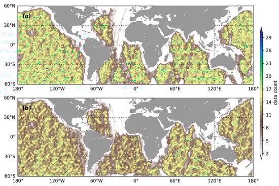
Figure 1.
Global data count of (a) Sentinel-1A (VV polarization) and (b) Sentinel-1B (HH polarization) WV1 (incidence angle of 23°) included in this study. The spatial bin is along the latitude and longitude, respectively.
To facilitate analysis of MACS relative to surface wind field (speed and direction), each SAR image collected in this study is systematically collocated with operational forecast winds distributed by the European Centre for Medium-Range Weather Forecasts (ECMWF). For simplicity, we straightforwardly take advantage of the forecast winds in the level 2 products of Sentinel-1 wave mode. The forecast winds are available at 3 h intervals and spatially gridded at 0.25° for both longitude and latitude [25]. The collocation criteria of SAR images and ECMWF winds are the nearest in time and in space. Figure 2a exhibits a histogram of collocated wind speed for the combinations of two incidence angles and both polarizations. The four groups have quite similar wind speed distribution curves, with similar peak wind speeds at 7 m/s. In general, the data count increases from low speed and reaches a maximum before dropping toward higher wind speeds. An exceptional observation is the distinctive bent curve at low wind speeds for the WV1 incidence angle. In addition to the curve shape, the quantitative values of the data count for each polarization and incidence angle are also close. The largest deviation of data count is found between HH WV2 and HH WV1 at a wind speed of 6 m/s, with a value of roughly up to 1000 images. The directional variation of MACS is a key aspect to address; thus, sufficient data count across the wind directions is essential. To demonstrate the distinct wind direction distribution at different wind speeds, Figure 2b presents the wind direction distribution at 7 m/s and 16 m/s. As shown at low wind speed, there are more data points across most of the wind direction bins, except those at cross-winds (90°) due to the geophysical wind circulations and satellite heading. In contrast, at 16 m/s, very few data points are accumulated. Therefore, our focus is placed within the wind speed range of [0 m/s, 15 m/s] in this study to ensure the value of our directional analysis.
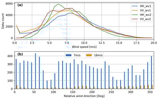
Figure 2.
(a) Histogram of collocated wind speed for both polarizations and incidence angles. (b) Histogram of wind direction at 7 m/s and 16 m/s for VV polarization at WV2.
2.2. Definition of MACS
Figure 3a presents a SAR image example with clear wave signatures of multiple wave systems. Ocean waves are characterized by the alternating bright and dark strips on the SAR imagery. As shown, a strong wave system in the direction from the bottom left to the upper right or opposite is the most obvious. As introduced in [23], the definition of MACS is based on SAR image cross-spectrum, which is estimated using single look complex imagery, as detailed in [26]. The processing steps include product calibration, bright targets removal, low-frequency signals suppression, and so on [26]. The fast Fourier transform is then applied to the partitioned tiles of each single look complex image at pixels to obtain the spectrum in the Doppler domain. This Doppler spectrum is then split into three non-overlapping parts to generate the sublook intensity images. The SAR image spectrum and cross-spectrum are then calculated with different combinations of sublooks, as shown in [23]. Note that the image spectrum represents the spectral analysis of autocorrelation for a given sublook, while cross-spectrum is for cross-correlation between different sublooks, as in [17]. Figure 3b,c exhibit the image spectrum and real part of the cross-spectrum, respectively. As shown, the wave system in the upper right and bottom left direction has the highest spectral energy of the other two wave systems. By comparison, the cross-spectrum in Figure 3c has lower spectral energy relative to the image spectrum in Figure 3b. This is expected due to the capability of cross-spectrum in suppressing speckle noise, as documented in [17]. The imaginary part of the cross-spectrum is given in Figure 3d, with the positive spectral energy depicting the true wave propagation direction. In this case, the strongest wave system propagates to the upper right of this image, as outlined by the spectral wave cluster in red at the peak wavenumber around 0.05 rad.
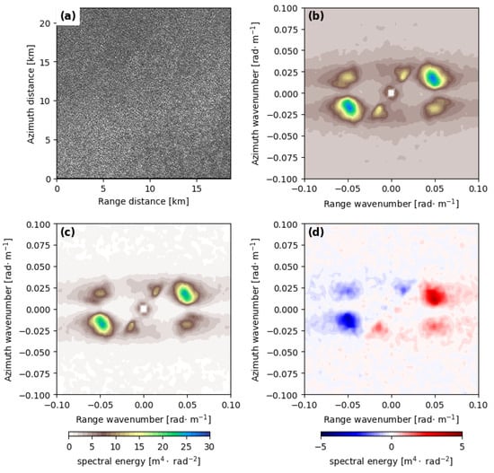
Figure 3.
(a) An example of SAR imagery acquired by Sentinel-1A at the incidence angle of 36° and VV polarization. Red lines give the prominent wave systems observed on the SAR image. (b) The computed image spectrum; (c) the real part and (d) the imaginary part of the cross-spectrum. Note that the positive imaginary part corresponds to the wave direction where it travels to.
A new spectrum-based radar parameter, MACS, has been introduced over the range-traveling intermediate ocean waves [23]. This novel parameter aims to capture the SAR image cross-spectra by filtering ocean waves within a specific wavelength range, precisely between 15 m and 20 m. To minimize nonlinear distortion induced by velocity bunching, the azimuth wavelength is selectively limited to values greater than 600 m, written as
where denotes the cross-spectrum, the overline denotes the ensemble average, and A is the area over which MACS is averaged, as presented in [23]. It is worth noting that in estimating SAR cross-spectra, the entire azimuth bandwidth is partitioned into three non-overlapping sub-looks, with a temporal interval of separating each sub-look, which equals a fourth of the SAR synthetic integration time. Consequently, MACS(n), which represents MACS estimated at various cross-spectrum intervals of , has been formulated. The resulting MACS(n) holds complex numerical values (except MACS(0), where the imaginary component remains constant at zero), with its magnitude referred to as MMACS(n) and the imaginary component as IMACS(n) in subsequent discussions. While previous research, as discussed in [23], has looked into the characterization of IMACS(1) and its relevance in portraying wind/wave climate, our focus in this paper will primarily center on the statistical analysis and applications of MMACS(0).
3. Statistics of MMACS(0)
By definition, MACS serves as a representation of RAR MTF-weighted intermediate wave spectral density. Consequently, the magnitude of MACS offers a direct insight into the quantitative aspects of RAR modulation. A better comprehension of RAR modulation holds key importance in enhancing the precision of retrieved ocean wave spectra derived from SAR images. The intermediate waves can be roughly regarded as being in an equilibrium state with the sea surface wind. Based on the findings in [21], the spectral density of intermediate waves is proportional to wind friction velocity, essentially the neutral wind speed. It is reasonable to assume that the wave spectral energy of intermediate ocean waves remains relatively constant at a given wind speed, irrespective of radar configurations such as the incidence and polarization. That is to say, the magnitude of MACS is only associated with the RAR modulation for different radar configurations. In this study, we first carried out the removal of noise contributions from SAR-observed MMACS(0). Subsequently, we explore the property of the noise-removed MMACS(0) as well as its application in the derivation of RAR modulation.
Speckle Noise
Most of the conventional representations of the SAR image rely on a multiplicative model to account for the speckle noise impact [27]. As formulated in [17], the contribution of speckle noise to the SAR image variance spectrum is a global noise floor independent of the wavenumber based on a white speckle noise assumption. A similar conclusion has been obtained in [28], but through an analytical derivation of the SAR image variance spectrum. In the former model, the speckle noise influence is linked to the transfer function of a SAR system as well as the normalized variance of the RAR modulation, while the latter model solely associates it with SAR spatial resolution. It is noteworthy that both models are predicated on the assumption of perfect sensitivity of the radar system, neglecting the sensor thermal noise. However, this idealized hypothesis does not hold in reality. The total noise contribution is supposed to encompass both the speckle noise and the system thermal noise and cannot be mitigated by simply removing a noise value estimated by the analytical SAR image spectrum theory. Given the difficulty in measuring the variance of the RAR image, we adopt a practical approach of assuming a global noise floor, as proposed in the latter model [28].
To derive the value of a global noise floor for each combination of polarization and incidence angle, we first filter out those SAR acquisitions with collocated wind direction blowing close to the radar line-of-sight axis to maximize the spectral level of MMACS(0). In specifics, all wind directions within from the radar range axis are included here, and the wind speed is then projected onto the range axis, termed as radial wind speed. Negative values correspond to upwind where the surface wind blows against the radar-pointing direction and negative values for the downwind configuration. The mean SAR-measured MMACS(0) variation relative to the radial wind speed is depicted in Figure 4a (solid curve). MMACS(0) exhibits a gradual decline over the range of 10 m/s to 4 m/s. The signal-to-noise ratio is quite low when the wind speed drops below 3 m/s. At low wind speeds, factors such as the presence of a surface surfactant or atmospheric turbulence may also introduce contamination to the surface scattering, leading to irregular variations in MMACS(0), as illustrated in Figure 4a. This irregularity poses challenges when attempting to determine the noise value defined at the 0 m/s wind speed. A careful examination of the descending trend of MMACS(0) at wind speeds exceeding 3 m/s reveals that the polynomial extrapolation is relatively practical to estimate the noise level. This MMACS(0) value is regarded as a universal noise floor, irrespective of wind speed. We therefore derive this value from SAR measurements to obtain an MMACS(0) free from noise.
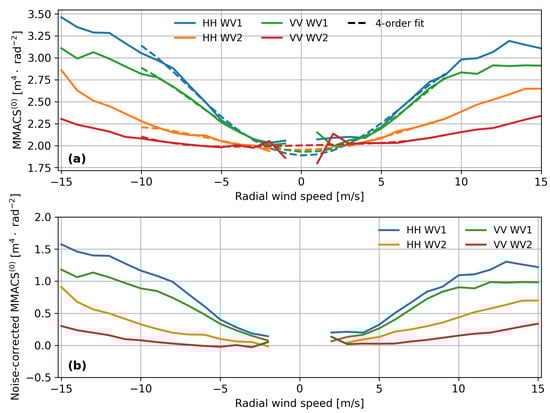
Figure 4.
(a) SAR-measured MMACS(0) versus the radial wind speed (wind directions ±10°). Solid lines are the measurements, and dashed lines are the fourth-order polynomial fit for SAR observations. The global noise floor is determined as the fitted MMACS(0) computed at the wind speed of 0 m/s. (b) MMACS(0) versus radial wind speed with removal of the global noise floor. Negative winds correspond to the upwind (wind blowing against the antenna).
To determine the optimal fit methods, various orders of the polynomial fit to SAR-measured MMACS(0) variation are tested. Though the curve visually follows a fourth-order polynomial variation, this method returns larger values at zero wind speed, leading to negative MMACS(0) after noise subtraction. The first-order polynomial fits are thus finally chosen given their lower residuals for each combination of polarization and incidence angle. The dashed curves in Figure 4a represent the first-order polynomial fits to SAR-measured MMACS(0) for wind speeds ranging from 3 m/s to 10 m/s. It is important to note that separate fits are carried out for downwind and upwind conditions, resulting in slightly different values at the wind speed of 0 m/s, as depicted in the plot. An average of these two values is adopted as the global noise floor for a given polarization and incidence angle. The specific noise floor values for VV WV1, VV WV2, HH WV1, and HH WV2 are 1.636 , 1.878 , 1.525 , and 1.823 , respectively. An interesting feature is that the noise floor is much higher for WV2 despite the larger spectral energy of WV1, which might be attributed to the fact that radar backscattering at large incidence angles is more subject to the influence of the background environment. The MMACS(0) corrected for noise is depicted in Figure 4b. Under low-wind conditions, MMACS(0) for WV1 continues to be affected by local contamination, a pattern not observed for WV2. Throughout the rest of this paper, the noise-free MMACS(0) is employed unless explicitly stated otherwise.
To illustrate how this noise removal affects the spectral energy across other wavenumbers, Figure 5 shows the spectral profile relative to the range wavenumber averaged over the azimuthal wavenumber bins, with the same MACS definition for both the image spectrum (red solid) and cross-spectrum (black solid). Because of the advantage of cross-spectrum in suppressing the thermal noise impact, the spectral energy at large wavenumbers is quite close to zero, indicating a high signal-to-noise ratio. By comparison, the image spectrum is subject to noise influence, with a spectral energy level fluctuating around 2 m4 for wavenumbers above 0.3 . The dashed red curve denotes the image spectrum profile after subtracting the noise floor. The step of noise removal makes the image spectrum close to the energy level of the cross-spectrum, which is particularly true at low wavenumbers around 0.1 . This is an indicator of the fact that the thermal noise floor is dependent on wavenumber, implying that a variant noise floor is needed to account for the noise removal in future studies.
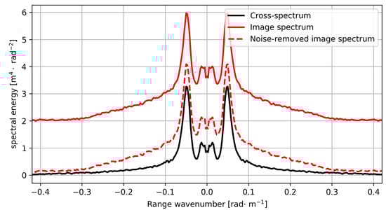
Figure 5.
An example of the spectral energy profile versus the range wavenumber averaged over the azimuth wavenumber extracted from SAR image shown in Figure 3.
3.1. Statistics of Noise-Free MMACS(0)
3.1.1. Azimuthal Modulation
For microwave radars, the normalized radar cross-section is commonly employed to characterize the backscattering of an illuminated sea surface. It represents the magnitude of scattering from centimeter-scale Bragg waves. Studies into the dual-polarization radar backscattering within C-band radar settings have thoroughly examined sea surface winds and incident angles through empirical geophysical model functions (GMF) [29,30]. Additionally, the polarization sensitivity of radar signal has been investigated through routine SAR acquisitions [31,32]. The existing GMF enables an examination of the sensitivity of derived RAR modulations to polarization channels. However, the complex process of extracting RAR modulation from SAR measurements has impeded its statistical validation using an empirical model. The MACS analysis provides a practical method to derive the RAR modulation from SAR observations. This enables the comparative examination of RAR modulation across different conditions, such as polarizations, incidence angles, and sea surface winds.
MMACS(0) are depicted concerning the collocated wind direction for VV and HH polarization at a wind speed of 9 m/s in Figure 6. As shown, its variation relative to wind direction roughly follows a cosine curve, similar to that of a radar cross-section. A fitting procedure to the observed MMACS(0) is conducted in terms of the harmonic functions, formulated as:
where the polarization channel of VV and HH is listed in the superscript pp. Figure 6a,b give the MMACS(0) variation for WV1. As illustrated, both VV and HH MMACS(0), in first order, exhibit analogous functional patterns concerning wind direction, similar to that of radar backscattering [32]. HH MMACS(0) slightly surpasses VV, attributed to higher RAR modulation in HH compared to VV [33]. In addition, HH MMACS(0) demonstrates a more pronounced azimuthal modulation compared to VV. As the incidence angle increases, the disparity between VV and HH MMACS(0) grows, similar to radar backscattering, with HH exhibiting greater MMACS(0) than VV. The MMACS(0) of WV2, depicted in Figure 6d, also shows a notable pattern with approximately half the period of a cosine function. Initially, it decreases, reaching its minimum at crosswind (270°), and then subsequently rises. This significant asymmetry between upwind and downwind is specific to WV2, irrespective of wind speed (curves for other wind speeds are not depicted here). Furthermore, the standard deviation (std) of MMACS(0) peaks at crosswinds and diminishes to a minimum at upwind and downwind (not illustrated here). The standard deviation (std) of HH MMACS(0) surpasses that of VV across all wind directions for WV2. This is anticipated since ocean waves at intermediate wavelengths typically exhibit nearly random fluctuations under crosswind conditions.
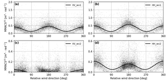
Figure 6.
MMACS(0) (top) at WV1 incidence angle for (a) VV polarization and (b) HH polarization; and (bottom) at WV2 incidence angle for (c) VV polarization and (d) HH polarization. The least-square fit using the form of Equation (2) to SAR measurements is given by the solid line in each plot. Note that the wind direction convention is 0° for upwind and 180° for downwind.
To further look into the two-dimensional characteristics of MMACS(0), the MMACS(0) is formulated for wind speed and direction. The wind speed bin size is 1 m/s in the range of [1 m/s, 15 m/s], and the wind direction bin is 5°. Figure 7 presents a graphical representation of MMACS(0) relative to wind speed and wind direction. The wind speed is delineated by concentric circles, each representing specific speeds (5 m/s, 10 m/s, 15 m/s) to facilitate a clear understanding of wind speed variations. Both discrete speed and direction bins provide a perspective on how MMACS(0) varies across different wind speeds and directions. Note that those data points corresponding to wind speeds lower than 2 m/s are neglected from the plot to enhance the clarity of data presentation. Each data point on the plot is derived by averaging the valid data within the specified bin, and this process is performed based on the equalized dataset to ensure robust and unbiased representation. In general, the two-dimensional pattern of MMACS(0) exhibits interesting features. An evident symmetry of WV1 MMACS(0) is observed from upwind to downwind, highlighting a balanced response across various wind conditions. The ratio of MMACS(0) approaches 1 from low to high wind speed for both HH and VV polarization in Figure 7a,c, respectively. In comparison, a notable asymmetry is shown for WV2, with an up-to-downwind ratio above 2 at different wind speeds. Consistent with Figure 6, MMACS(0) in HH polarization is much larger than that in VV polarization. To dig deeper into the azimuthal modulation of MMACS(0), the following analysis will focus on the upwind–downwind asymmetry and the upwind–crosswind asymmetry. These metrics shall provide a more detailed understanding of how MMACS(0) behaves under different wind conditions.
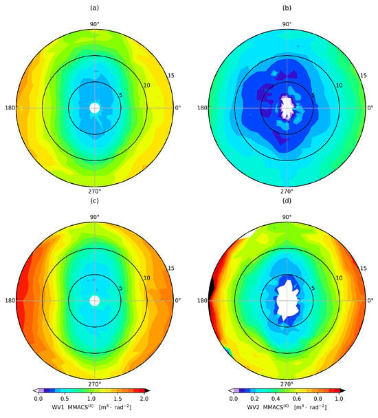
Figure 7.
The two-dimensional plot displays MMACS(0) for (a) HH WV1; (b) VV WV1; (c) HH WV2; and (d) VV WV2. The concentric circles indicate wind speeds ranging from inner to outer circles as 5 m/s, 10 m/s, and 15 m/s, respectively. MMACS(0) is depicted by background color. A wind direction of 0° corresponds to upwind (wind blowing against the direction of the antenna).
3.1.2. Upwind-to-Downwind and -Crosswind Asymmetry
SAR-measured radar backscattering is predominantly influenced by the backscattering associated with the sea surface roughness, primarily composed of centimeter-scale Bragg waves. The azimuthal modulation of radar backscattering serves as a valuable tool for characterizing the azimuthal distribution of these Bragg waves. Drawing a parallel from this methodology, MMACS(0) is employed to reveal the azimuthal distribution of range-traveling intermediate waves. In alignment with the established conventions, this study adopts the definitions of upwind-to-crosswind asymmetry and upwind-to-downwind asymmetry as outlined in [32]:
where are fit coefficients in the form of Equation (2) for MMACS(0), respectively. The upwind-to-crosswind asymmetry of MMACS(0), as illustrated in Figure 8, exhibits a notable sensitivity to changes in wind speed, given a specific incidence angle and polarization. Specifically, in the case of WV1, the MMACS(0) upwind-to-crosswind asymmetry displays a gradual increase with increasing wind speeds. While for WV2, the upwind-to-crosswind asymmetry of MMACS(0) does not exhibit significant variations across different wind speeds. Further analysis reveals distinctive patterns in MMACS(0) upwind-to-crosswind asymmetry concerning both HH and VV polarizations at higher wind speeds (larger than 8 m/s) for WV1. This contrast becomes less pronounced as wind speed drops below 10 m/s. The observed difference in MMACS(0) upwind-to-crosswind asymmetry between HH and VV polarizations at higher wind speeds suggests the influence of factors such as RAR MTF in both polarizations.
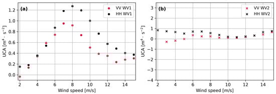
Figure 8.
Upwind-to-crosswind asymmetry of MMACS(0) for (a) WV1 and (b) WV2 as a function of wind speed.
The analysis of upwind-to-downwind asymmetry features in MMACS(0) is presented in Figure 9. A thorough examination of the upwind-to-downwind asymmetry variation relative to radial wind speed shows a distinctly different asymmetry for a small incidence angle of WV1. Specifically, the upwind-to-downwind asymmetry values for MMACS(0) in WV1 predominantly exhibit negative values, indicating a consistent trend across the dataset. Notably, a strong similarity is observed between HH and VV polarizations in terms of upwind-to-downwind asymmetry patterns. In comparison, the upwind-to-downwind asymmetry variation at the 36° incidence angle of WV2 displays different features. In WV2, the upwind-to-downwind asymmetry values of MMACS(0) are mostly larger in VV polarization than in HH polarization. This result can be attributed to the lower level of VV-polarized MMACS(0), as depicted in Figure 6 and Figure 7. This asymmetry from the upwind to downwind configuration is relatively more evident in WV2. The azimuthal modulation analysis of MMACS(0) sheds light on the complex SAR mapping of ocean waves at a given wavenumber relying on the radar configurations and wind conditions, contributing to the understanding of data interpretation in ocean wave observations.
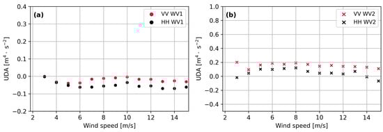
Figure 9.
The same as Figure 5 but for upwind-to-downwind asymmetry.
4. RAR Modulation Derived from MMACS(0)
In this section, we first introduce the procedure of simulating an SAR image cross-spectrum in terms of the nonlinear SAR imaging principle. SAR-measured MMACS(0) and that simulated with the input of RAR MTF derived from empirical GMF are compared and assessed. A statistical ratio of RAR MTF is derived relative to the empirical RAR MTF through a pointwise comparison of SAR measurement and the simulation.
4.1. Simulation of SAR Image Cross-Spectra
The SAR imaging principle of ocean waves has been well documented to be a nonlinear process, as presented in [17]. Here, we take advantage of the mapping model from the ocean wave spectrum for the SAR image cross-spectrum. As reported in [17], the mapping relation is mainly composed of three processes: tilt modulation, hydrodynamic modulation, and velocity bunching. Each SAR image is partitioned into three sublooks, and the closed-form formulation of a SAR image cross-spectrum for the mth and nth sublook is written as:
where the subscripts d and I in are the MTF of velocity bunching and RAR modulation, respectively; denotes the azimuthal wavenumber along the satellite flying direction; and in Equation (5) is the correlation function of each modulation component relating to the directional ocean wave spectrum by
where the term describes the modulation transfer functions of tilt modulation and the nonlinear velocity bunching. The following expression for the velocity bunching modulation is used
where is the SAR slant-range-to-velocity ratio. The RAR modulation composed of the tilt and hydrodynamic modulation is written as
where
where is calculated based on CSARMOD [32] with the collocated wind speed and direction as well as the radar incidence from Sentinel-1 annotation data. In this study, we use the collocated ocean wave spectra provided by the third-generation wave spectral model WAVEWATCH III with the wind forcing from ECMWF and the parameterizations of [34]. Each Sentinel-1 wave mode image is collocated with a directional wave spectrum, with the model wave spectra composed of 32 wave frequency bins ranging from 0.0056 rad·m−1 to 2.0632 rad·m−1 and 24 wave directions with a direction bin of 15°. It is worth mentioning that the minimum wavelength of sea surface waves of the model wave spectrum is 3.045 m, slightly smaller than the Sentinel-1 spatial resolution.
4.2. Derived RAR Modulation
We first plot values of RAR MTF versus wind speeds estimated using empirical GMF CSARMOD [32] through in Figure 10a for VV and HH polarizations, respectively. For comparison, we also plot the RAR MTF estimated using the empirical GMF of CMOD5.N [29] in Figure 10a. As shown, the RAR MTF obtained by CSARMOD is generally in good agreement with that of CMOD5.N for VV polarization. The RAR MTF is larger in HH polarization than in VV polarization, consistent with the feature in Figure 7. The overall SAR image cross-spectrum is simulated in terms of the SAR mapping principle from the ocean wave spectrum using the RAR MTF estimated by CSARMOD. MMACS(0) is then extracted from the simulated SAR image cross-spectrum. The comparison of MMACS(0) between SAR observation and the simulation for WV1 and WV2 is presented in Figure 10b,c, respectively. SAR-measured MMACS(0) is generally larger than that of the simulation at both WV1 and WV2 for each polarization. For instance, the value of SAR-measured MMACS(0) is three times as high as the simulated MMACS(0) for the combination of VV polarization and WV1 at the wind speed of upwind 10 m/s. While for WV2, SAR measurements are mostly consistent with the simulation of MMACS(0) at upwind wind speeds lower than 10 m/s as plotted in Figure 10c. This implies that the RAR MTF used to simulate SAR image cross-spectrum through the empirical GMF is only able to reproduce to a certain extent the true modulation for low to median wind speed (<10 m/s). In other words, the empirical derivation of RAR MTF in terms of is deficient in representing the true RAR modulation across a broad range of wind speeds.
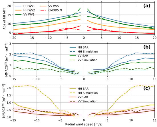
Figure 10.
(a) RAR MTF derived from the empirical GMF using . The solid lines are the results using CSARMOD, and the dashed lines using CMOD5. Comparisons of SAR-measured MMACS(0) (solid curves) and the simulation (dashed curves) at the incidence angle of (b) WV1 and (c) WV2 are plotted, respectively.
The insufficiency of using empirical GMF to estimate RAR modulation can be explained in theory. In terms of the composite scattering theory of sea surface scattering, as in [35], the radar-received backscattering magnitude could be formulated by the slope of a long ocean wave up to the second order by:
where the nominal radar incidence angle is denoted by , and denotes the variation of local incidence angle associated with the surface slope of long ocean waves. However, the of any empirical GMF (CSARMOD or CMOD5.N) is presented as the averaged radar backscattering signal (SAR measured or scatterometer measured) to a reduced spatial resolution, and it can be factored as:
where is expressed as a function of the instantaneous sea surface height , and its local average is represented by . As listed on the right of the equation, the first-order tilt modulation characterized by is averaged out in the local mean field. In other words, the RAR MTF derived from the empirical GMF is not able to capture the first-order tilt modulation properly. SAR spectral analysis of ocean waves as defined by MACS encompasses the modulation of local radar backscattering at both first and second order. This creates the disagreement between the SAR-measured and simulated MMACS(0), as shown in Figure 10b,c. Given the fact that MMACS(0) shows the best consistency for WV2 at the upwind configuration, it shall be speculated that smaller incidence angles expect a more significant contribution from the first-order tilt modulation, particularly at the downwind configuration.
It should be noted that the derivation of the first-order tilt MTF from SAR-measured MMACS(0) is not straightforward. As an alternative, a practical method is proposed to estimate the RAR MTF in terms of the direct comparison of MMACS(0) between SAR measurement and the simulation. By its definition, MMACS(0) could be approximated by the quasi-linear mapping of ocean waves as formulated in [4]:
where the modulation of velocity bunching is formulated in the first exponential with the term representing the azimuth cutoff value. The other symbols are the same as Equation (5). As documented in previous studies, azimuth cutoff is mostly a function of sea surface wind vector (speed and direction) and incidence angle formulated by SAR slant-range-to-velocity ratio [36]. Since MMACS(0) is defined close to the range axis with the azimuth wavelength longer than 600 m, the RAR MTF dominates over the contribution of velocity bunching . For a given sea state, variations of MMACS(0) are mainly associated with variations of RAR MTF. As an approximation, the nonlinear part in Equation (12) can be ignored, and MMACS(0) can then be simplified to the form of
The term associated with the azimuth cutoff is denoted by F for simplicity here. The ratio of SAR-measured MMACS(0) relative to the simulation could be written as
where the symbols of T and E indicate SAR-measured RAR modulation and the derived RAR modulation using empirical GMF, respectively.
The ratio of is plotted relative to the radial wind speed in Figure 11a. As shown, this ratio is a constant from low to high wind speed for each combination of incidence angle and polarization. A smaller incidence angle of WV1 shows a larger ratio for both polarizations, indicating the underestimation of the empirical RAR MTF derived from radar backscattering GMF. In comparison, an overestimation of RAR modulation is observed for WV2, particularly at downwind. In a straightforward comparison of this ratio between the upwind and downwind, a difference in the order of 30% is observed in the RAR MTF values. The ratio variation relative to azimuth wind direction at a wind speed of 10 m/s is presented in Figure 11b. An evident difference in the azimuthal modulation of this ratio is observed in VV and HH polarization, as shown. For VV polarization at two incidence angles, local maxima of the ratio occur at upwind/downwind (wind direction of 0°/180°). For HH polarization, the local maxima are found at the two crosswinds of 90°/270°. It is worth pointing out that the above results are obtained based on the assumption that the velocity bunching is constant for the definition of MMACS(0). This is only to demonstrate the potential of using MMACS(0) to derive RAR modulation from a statistical point of view. Despite rough adjustments, this provides a new insight into refining the insufficient RAR MTF estimated using the empirical GMF, particularly in reproducing the up-to-downwind asymmetry.
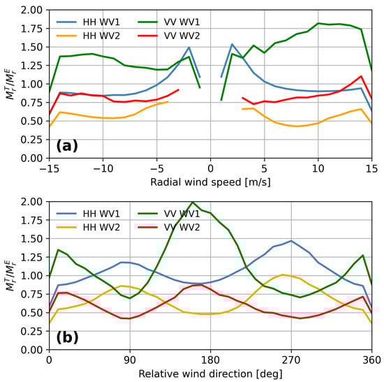
Figure 11.
The RAR MTF ratio as derived using Equation (14) concerning (a) the radial wind speed and (b) the relative wind direction.
The imprecise estimation of RAR modulation through empirical GMF introduces inaccuracies in the inversion of ocean wave spectra from SAR images. It is widely acknowledged that RAR modulation, denoted as , holds global applicability across all wavenumbers for a given radar configuration and environmental conditions. To illustrate this, we examine a specific case involving a wind speed of 7 m/s and upwind conditions at an incidence angle of 23°. In Figure 11, the empirical RAR modulation is estimated as 11.6, while the true modulation is tuned to 18.6 in terms of the ratio. The results indicate a discrepancy, revealing that the inversion of significant wave height using the empirical RAR modulation leads to an overestimation of roughly 0.15 m. This emphasizes the critical role of accurate RAR modulation estimation in SAR-based ocean wave spectrum inversions. Remarkably, investigation of the performance of ocean swell inversion concerning wind direction has received limited attention in previous studies. In this context, the study of intermediate waves emerges as a significant avenue to bridge this gap. This is attributed to the unique sensitivity of intermediate waves to both wind speed and wind direction, providing an insightful perspective that is worth further investigation.
5. Conclusions
SAR has become an invaluable tool in oceanographic remote sensing due to its exceptional ability to measure two-dimensional ocean wave spectra. This capability is crucial for deriving key sea state parameters, such as wave height, frequency, and direction, which are essential for understanding ocean dynamics. The Sentinel-1 mission, with its high spatial resolution and comprehensive global coverage of the open ocean, provides an ideal platform for such investigations. In particular, we focus on the characteristics of intermediate ocean waves with wavelengths around 20 m, a crucial wavelength range that significantly influences the dynamics of the open ocean. To explore these intermediate waves, we utilize a systematically collocated dataset that combines SAR observations from various locations and times, ensuring a diverse and representative set of conditions. This dataset allows for a more thorough examination of the spatial and temporal variability of intermediate waves. A major advancement in our research is the application of the MACS radar parameter, which has been specifically designed to characterize range-traveling intermediate waves as observed within SAR image cross-spectra. The cross-spectrum formulation reduces speckle noise by taking advantage of phase coherence between multiple sub-looks, providing a more stable estimation of intermediate wave spectra compared to the conventional image spectrum. While the conventional image spectrum retains the full spectral content, it is more subject to random noise and speckle-induced variations, which can contaminate wave-related modulations. The cross-spectrum approach, therefore, offers a refined representation of ocean wave characteristics, particularly in cases where the signal-to-noise ratio is a limiting factor in conventional spectral analysis. By applying MACS, we can more accurately distinguish and analyze these waves, enhancing our understanding of their behavior and their role in sea state dynamics.
The MACS parameter provides unique insights into the interactions between ocean waves and atmospheric conditions, offering a distinctive reflection of dependencies on both wind speed and wind direction. One of the key features of MACS is its azimuthal modulation of wind direction, which offers valuable information regarding the spread function of the ocean wave spectrum. This modulation allows for a more detailed understanding of how wind patterns influence wave propagation and energy distribution across the ocean surface. Moreover, the inherent up-to-downwind asymmetry captured by MACS plays a critical role in quantifying the modulation of RAR, a phenomenon that has traditionally been challenging to measure. By effectively capturing this asymmetry, MACS provides a new avenue for more accurate assessments of ocean wave behavior under varying wind conditions. Additionally, the polarization sensitivity of MACS significantly enhances our understanding of polarimetric SAR imaging of ocean waves. This capability enables more precise differentiation of wave features, leading to improved interpretations of ocean surface dynamics in SAR observations. As a result, MACS serves as a powerful tool for advancing SAR-based oceanography, with applications in both theoretical studies and practical remote sensing systems.
RAR modulation plays a crucial role in achieving precise inversion of ocean wave spectra from SAR images. Through an in-depth analysis of the MMACS with regard to the radial wind speed, our findings indicate a substantial underestimation of RAR modulation when relying on empirical GMF. This empirical estimation fails to capture the up-to-downwind asymmetry inherent in RAR modulation. The evaluation of hydrodynamic modulation in addressing this asymmetry requires careful consideration and further investigation. The observed underestimation (or overestimation) of RAR modulation holds significant implications, leading to corresponding inaccuracies in the estimation of ocean wave spectra. This study offers valuable insights into enhancing the accuracy of RAR modulation estimates by integrating SAR observations with simulation results. However, it should be mentioned that the estimation accuracy of intermediate wave spectra using MACS is influenced by multiple factors, including wind speed, wind direction, and polarization, all of which play a crucial role in radar modulation. MACS, defined as the SAR image cross-spectrum over a specific wavenumber range, captures the modulated ocean wave spectrum and reflects the interaction between the ocean surface and radar signals. While ocean wave spectra may exhibit statistical consistency for given wind vectors and radar configurations, variations in these environmental parameters lead to distinct changes in MACS values. For instance, at a fixed wind speed and direction, the modulation induced by real aperture radar is typically stronger in HH polarization than in VV polarization. Similarly, under a given polarization, wind speed and direction exert different influences on the radar modulation function, making it challenging to determine a single dominant factor. The complex interplay between these variables highlights the need for further investigation to quantify their relative contributions, which could be achieved through controlled simulations and multi-polarization SAR observations.
Author Contributions
Conceptualization, H.L.; methodology, H.L.; formal analysis, K.L. and H.L.; investigation, K.L. and H.L.; writing—original draft preparation, K.L.; writing—review and editing, H.L. All authors have read and agreed to the published version of the manuscript.
Funding
This study is supported by the National Science Foundation of China under grant number 42476182.
Data Availability Statement
The original contributions presented in this study are included in the article. Further inquiries can be directed to the corresponding author.
Acknowledgments
Copernicus data (2017) are used. The ECMWF forecast winds were obtained in the framework of the Sentinel-1 Mission Performance Center and are publicly available via www.ecmwf.int, accessed on 1 December 2024.
Conflicts of Interest
The authors declare no conflicts of interest.
References
- Elfouhaily, T.; Chapron, B.; Katsaros, K.; Vandemark, D. A unified directional spectrum for long and short wind-driven waves. J. Geophys. Res. Oceans 1997, 102, 15781–15796. [Google Scholar] [CrossRef]
- Ryabkova, M.; Karaev, V.; Guo, J.; Titchenko, Y. A Review of Wave Spectrum Models as Applied to the Problem of Radar Probing of the Sea Surface. J. Geophys. Res. Oceans 2019, 124, 7104–7134. [Google Scholar] [CrossRef]
- Jackson, C.R.; Apel, J.R. (Eds.) Synthetic Aperture Radar Marine User’s Manual; U.S. Department of Commerce National Oceanic and Atmospheric Administration, National Environmental Satellite, Data, and Information, Service Office of Research and Applications: Washington, DC, USA, 2004. [Google Scholar]
- Hasselmann, K.; Hasselmann, S. On the nonlinear mapping of an ocean wave spectrum into a synthetic aperture radar image spectrum and its inversion. J. Geophys. Res. 1991, 96, 10713–10729. [Google Scholar] [CrossRef]
- Kudryavtsev, V.; Kozlov, I.; Chapron, B.; Johannessen, J.A. Quad-polarization SAR features of ocean currents. J. Geophys. Res. Oceans 2014, 119, 6046–6065. [Google Scholar] [CrossRef]
- Alpers, W.; Hennings, I. A theory of the imaging mechanism of underwater bottom topography by real and synthetic aperture radar. J. Geophys. Res. 1984, 89, 10529–10546. [Google Scholar] [CrossRef]
- Ardhuin, F.; Collard, F.; Chapron, B.; Girard-Ardhuin, F.; Guitton, G.; Mouche, A.; Stopa, J.E. Estimates of ocean wave heights and attenuation in sea ice using the SAR wave mode on Sentinel-1A. Geophys. Res. Lett. 2015, 42, 2317–2325. [Google Scholar] [CrossRef]
- Ardhuin, F.; Stopa, J.; Chapron, B.; Collard, F.; Smith, M.; Thomson, J.; Doble, M.; Blomquist, B.; Persson, O.; Collins, C.O.; et al. Measuring ocean waves in sea ice using SAR imagery: A quasi-deterministic approach evaluated with Sentinel-1 and in situ data. Remote Sens. Environ. 2017, 189, 211–222. [Google Scholar] [CrossRef]
- Huang, B.; Li, X. Study on Retrievals of Ocean Wave Spectrum by Spaceborne SAR in Ice-Covered Areas. Remote Sens. 2022, 14, 6086. [Google Scholar] [CrossRef]
- Pramudya, F.S.; Pan, J.; Devlin, A.T.; Lin, H. Enhanced Estimation of Significant Wave Height with Dual-Polarization Sentinel-1 SAR Imagery. Remote Sens. 2021, 13, 124. [Google Scholar] [CrossRef]
- Wang, H.; Mouche, A.; Husson, R.; Grouazel, A.; Chapron, B.; Yang, J. Assessment of Ocean Swell Height Observations from Sentinel-1A/B Wave Mode against Buoy In Situ and Modeling Hindcasts. Remote Sens. 2022, 14, 862. [Google Scholar] [CrossRef]
- Vachon, P.W.; Krogstad, H.E.; Paterson, J.S. Airborne and spaceborne synthetic aperture radar observations of ocean waves. Atmos.-Ocean 1994, 32, 83–112. [Google Scholar] [CrossRef]
- Engen, G.; Vachon, P.W.; Johnsen, H.; Dobson, F.W. Retrieval of ocean wave spectra and RAR MTF’s from dual-polarization SAR data. IEEE Trans. Geosci. Remote Sens. 2000, 38, 391–403. [Google Scholar] [CrossRef]
- Collard, F.; Ardhuin, F.; Chapron, B. Monitoring and analysis of ocean swell fields from space: New methods for routine observations. J. Geophys. Res. Oceans 2009, 114, C07023. [Google Scholar] [CrossRef]
- Zhang, B.; Perrie, W.; He, Y. Remote sensing of ocean waves by along-track interferometric synthetic aperture radar. J. Geophys. Res. Oceans 2009, 114, 10015. [Google Scholar] [CrossRef]
- Stopa, J.E.; Ardhuin, F.; Husson, R.; Jiang, H.; Chapron, B.; Collard, F. Swell dissipation from 10 years of Envisat advanced synthetic aperture radar in wave mode. Geophys. Res. Lett. 2016, 43, 3423–3430. [Google Scholar] [CrossRef]
- Engen, G.; Johnsen, H. SAR-ocean wave inversion using image cross spectra. IEEE Trans. Geosci. Remote Sens. 1995, 33, 1047–1056. [Google Scholar] [CrossRef]
- Hasselmann, S.; Brüning, C.; Hasselmann, K.; Heimbach, P. An improved algorithm for the retrieval of ocean wave spectra from synthetic aperture radar image spectra. J. Geophys. Res. Oceans 1996, 101, 16615–16629. [Google Scholar] [CrossRef]
- Jiang, H.; Mouche, A.; Wang, H.; Babanin, A.V.; Chapron, B.; Chen, G. Limitation of SAR Quasi-Linear Inversion Data on Swell Climate: An Example of Global Crossing Swells. Remote Sens. 2017, 9, 107. [Google Scholar] [CrossRef]
- Jacobsen, S.; Høgda, K.A. Estimation of the real aperture radar modulation transfer function directly from synthetic aperture radar ocean wave image spectra without a priori knowledge of the ocean wave height spectrum. J. Geophys. Res. 1994, 99, 14291–14302. [Google Scholar] [CrossRef]
- Phillips, O.M. Spectral and statistical properties of the equilibrium range in wind-generated gravity waves. J. Fluid Mech. 1985, 156, 505–531. [Google Scholar] [CrossRef]
- Li, J.G.; Holt, M. Comparison of Envisat ASAR Ocean Wave Spectra with Buoy and Altimeter Data via a Wave Model. J. Atmos. Ocean. Technol. 2009, 26, 593–614. [Google Scholar] [CrossRef]
- Li, H.; Chapron, B.; Mouche, A.; Stopa, J.E. A New Ocean SAR Cross-Spectral Parameter: Definition and Directional Property Using the Global Sentinel-1 Measurements. J. Geophys. Res. Oceans 2019, 124, 1566–1577. [Google Scholar] [CrossRef]
- Torres, R.; Snoeij, P.; Geudtner, D.; Bibby, D.; Davidson, M.; Attema, E.; Potin, P.; Rommen, B.; Floury, N.; Brown, M.; et al. GMES Sentinel-1 mission. Remote Sens. Environ. 2012, 120, 9–24. [Google Scholar] [CrossRef]
- Sentinel-1 Mission Performance Center. Sentinel-1 Product Specification; Technical Report S1-RS-MDA-52-7441; ESA Unclassified—For Official Use; European Space Agency: Paris, France, 2020. [Google Scholar]
- Johnsen, H.; Collard, F. Sentinel-1 Ocean Swell Wave Spectra (OSW) Algorithm Definition; Technical Report; Norut: Tromsø, Norway, 2009. [Google Scholar]
- Hasselmann, K.; Raney, R.K.; Plant, W.J.; Alpers, W.; Shuchman, R.A.; Lyzenga, D.R.; Rufenach, C.L.; Tucker, M.J. Theory of synthetic aperture radar ocean imaging: A MARSEN view. J. Geophys. Res. 1985, 90, 4659–4686. [Google Scholar] [CrossRef]
- Schulz-Stellenfleth, J.; Lehner, S. A noise model for estimated synthetic aperture radar look cross spectra acquired over the ocean. IEEE Trans. Geosci. Remote Sens. 2005, 43, 1443–1452. [Google Scholar] [CrossRef]
- Hersbach, H.; Stoffelen, A.; de Haan, S. An improved C-band scatterometer ocean geophysical model function: CMOD5. J. Geophys. Res. Oceans 2007, 112, 03006. [Google Scholar] [CrossRef]
- Stoffelen, A.; Verspeek, J.A.; Vogelzang, J.; Verhoef, A. The CMOD7 Geophysical Model Function for ASCAT and ERS Wind Retrievals. IEEE J. Sel. Top. Appl. Earth Obs. Remote Sens. 2017, 10, 2123–2134. [Google Scholar] [CrossRef]
- Zhang, B.; Perrie, W.; He, Y. Wind speed retrieval from RADARSAT-2 quad-polarization images using a new polarization ratio model. J. Geophys. Res. Oceans 2011, 116, 08008. [Google Scholar] [CrossRef]
- Mouche, A.; Chapron, B. Global C-Band Envisat, RADARSAT-2 and Sentinel-1 SAR measurements in copolarization and cross-polarization. J. Geophys. Res. Oceans 2015, 120, 7195–7207. [Google Scholar] [CrossRef]
- Alpers, W.R.; Ross, D.B.; Rufenach, C.L. On the detectability of ocean surface waves by real and synthetic aperture radar. J. Geophys. Res. Oceans 1981, 86, 6481–6498. [Google Scholar] [CrossRef]
- Ardhuin, F.; Rogers, E.; Babanin, A.V.; Filipot, J.F.; Magne, R.; Roland, A.; van der Westhuysen, A.; Queffeulou, P.; Lefevre, J.M.; Aouf, L.; et al. Semiempirical Dissipation Source Functions for Ocean Waves. Part I: Definition, Calibration, and Validation. J. Phys. Oceanogr. 2010, 40, 1917–1941. [Google Scholar] [CrossRef]
- Valenzuela, G.R. Theories for the interaction of electromagnetic and oceanic waves—A review. Bound.-Layer Meteorol. 1978, 13, 61–85. [Google Scholar] [CrossRef]
- Kerbaol, V.; Chapron, B.; Vachon, P.W. Analysis of ERS-1/2 synthetic aperture radar wave mode imagettes. J. Geophys. Res. Oceans 1998, 103, 7833–7846. [Google Scholar] [CrossRef]
Disclaimer/Publisher’s Note: The statements, opinions and data contained in all publications are solely those of the individual author(s) and contributor(s) and not of MDPI and/or the editor(s). MDPI and/or the editor(s) disclaim responsibility for any injury to people or property resulting from any ideas, methods, instructions or products referred to in the content. |
© 2025 by the authors. Licensee MDPI, Basel, Switzerland. This article is an open access article distributed under the terms and conditions of the Creative Commons Attribution (CC BY) license (https://creativecommons.org/licenses/by/4.0/).