1. Introduction
Land cover survey and mapping is an important basis for optimizing agricultural management [
1], improving the accuracy of forest cover estimation [
2], and promoting sustainable development [
3]. Current land cover products are mainly divided into two technological paradigms: The first is single-year high-precision reference datasets (e.g., GLC_FCS30D), which realize subpixel-level classification through multi-source data fusion. Although these do not explicitly construct time series, multi-baseline-year comparison can indirectly support dynamic land cover analysis. The second category is local temporal dynamic datasets, which use standardized algorithms to generate continuous temporal products. Examples include the European Space Agency Climate Change Initiative (ESA CCI), which has provided annual composite data at 300 m resolution since 1992, and Dynamic World, which updates 10 m resolution images every 5 days through the Long Short-Term Memory (LSTM) model. These two kinds of technological breakthroughs make dynamic land cover analysis possible and profoundly reshape the theoretical and methodological system of land change research.
Dynamic land cover data, with the advantages of multi-scale and high-frequency monitoring, are driving the enhancement of management efficiency across various fields [
4,
5]. In recent years, with the continuous advancement of remote sensing technology and the diversification of data acquisition methods, the number and types of global time-series land cover datasets have shown a rapid growth trend. These datasets originate from different satellite sensors, research institutions, and projects, and they vary in spatial resolution, temporal resolution, and classification systems. In addition to the aforementioned datasets, such as GLC_FCS30D, ESA CCI, and Dynamic World, there are also products like MODIS MCD12Q1 and Esri Land Cover, each with unique data characteristics and application scenarios. Many global time-series land cover datasets now span long time periods, providing rich data support for studying long-term land cover changes. For instance, the ESA CCI has been offering annual composite land cover data at 300 m resolution since 1992. Moreover, datasets like Dynamic World make it possible to conduct real-time monitoring and short-term change analysis through more frequent update cycles, such as updating 10 m resolution imagery every five days. However, faced with the multitude of global time-series land cover datasets, users often find themselves perplexed in practical applications. Differences in classification accuracy, temporal consistency, and spatial resolution among datasets make it difficult for users to determine which dataset is most suitable for their specific research or application needs.
There are several deficiencies in the current evaluation of global time-series land cover datasets, which are primarily manifested in the following aspects:
- (1)
Lack of systematic comparison. At present, there is a relative scarcity of systematic comparisons regarding the classification accuracy and temporal consistency of different land cover datasets, along with a lack of unified evaluation standards and methods. Different studies often employ varying evaluation metrics and data samples, resulting in outcomes that are difficult to compare and integrate. Moreover, there is a lack of systematic comparison between geographical regions, with most research focusing on specific regions or the global scale, neglecting the differences and connections between regions. For instance, Yang et al. [
6] proposed to assess the reliability of time-series land cover products through Hidden Markov Model (HMM) joint probability, combining classification performance with spatiotemporal relationships to validate the land cover data in the Poyang Lake Ecological and Economic Zone. Narumasa et al. [
7] developed a spatiotemporal accuracy assessment method based on Geographically Weighted Logistic Regression (Logistic GWR) for the rapidly urbanizing Jakarta Metropolitan Area using MODIS time-series data from 2001 to 2013. While this regionalized validation framework can reveal local accuracy heterogeneity, it relies on a single dataset (MODIS) and lacks an established cross-resolution alignment protocol, preventing the support of spatiotemporal comparability analysis across multiple products. Therefore, a global-scale evaluation of the temporal consistency of dynamic land cover datasets remains lacking.
- (2)
Insufficiency in dynamic assessment: Despite the increasing number of dynamic land cover datasets, the systematic evaluation of their dynamic characteristics, particularly in terms of temporal consistency, is lagging. Current assessments primarily focus on static classification accuracy. For instance, Herold et al. [
8] conducted an analysis of spatial consistency and uncertainty for global-scale land cover products, revealing the limitations of current 1 km resolution products in complex landscapes by harmonizing classification standards across multiple datasets. Tsendbazar et al. [
9] systematically assessed the strengths and limitations of existing datasets in supporting various application scenarios from a user’s perspective. However, many studies overlook the coherence and stability of datasets over time, which are crucial for monitoring land cover changes and predicting future trends. Currently, there is a lack of an effective validation framework to assess this key attribute. For example, ensuring that the land cover classification results of long-time-series datasets are consistent and comparable over time is an urgent issue that needs to be addressed.
- (3)
Deficiencies in technical research: Existing studies still fall short in addressing issues such as scale dependency differences, uncertainty quantification, and the fusion of multi-source datasets.
Firstly, the impact of scale effects on data accuracy shows a cascading amplification characteristic between coarse-resolution and high-resolution products. Moody et al. [
10] systematically revealed the cascading effects of spatial-resolution differences on land cover classification accuracy, noting that coarse-resolution datasets may significantly underestimate the proportion of rare land classes in fragmented landscapes, such as wetlands and urban green spaces. Tudesque et al. [
11] found evidence in the Adour-Garonne river basin that errors in land cover classification, which vary with scale, not only occur in the classification, but also greatly harm subsequent applications by misaligning how land classes respond to the environment, highlighting the need for a validation method that ensures spatial consistency across different resolutions for the accuracy of ecological models. There is a lack of effective methods for comparing and fusing datasets of different resolutions, with coarse- and fine-resolution products differing in information expression and application requirements. How to achieve accurate conversion and integration across scales remains an area in need of further research.
Secondly, the quantification of uncertainty in the dynamics of time-series land cover is underrepresented in existing studies, which often focus on the classification accuracy of static data. For example, Waśniewski et al. [
12] improved the classification accuracy of Sentinel-2 data through optimized sample selection and DEM fusion, but the validation relied solely on single-phase confusion matrices (such as Kappa coefficients), without assessing the logical rationality of inter-annual changes. Abercrombie et al. [
13] significantly reduced the magnitude of spurious inter-annual changes in coarse-resolution (300–500 m) land cover products by constraining label transition probabilities with HHM. However, such methods are still limited to internal time-smoothing optimizations within a single dataset and do not address the issue of cross-resolution comparability between multi-source products, leading to challenges in ensuring the compatibility and consistency of different-resolution data in land cover dynamics monitoring. Existing research predominantly focuses on statistical descriptions of classification accuracy, with less attention given to uncertainty in the temporal dimension, which lacks a systematic validation framework to comprehensively assess data reliability.
Finally, research on the fusion of multi-source datasets is relatively weak. To improve the cross-comparability of multi-source land cover products, the academic community has investigated harmonization techniques for multi-source land cover datasets, with classification system calibration and resolution resampling trade-offs being key aspects of this process [
14]. In terms of classification system calibration, Liu et al. [
15] released the GLASS-GLC global long-time-series land cover product, which improved the annual average classification accuracy to 82.81% by constructing a full-season universal sample library and temporal–spatial consistency post-processing techniques. In terms of resolution coordination, when fusing Sentinel-2 and Landsat-8 data, they found that bilinear interpolation led to a decrease in user accuracy of 8–12% in farmland boundary representation and proposed a sub-pixel algorithm based on spectral unmixing to mitigate mixed-pixel errors. However, such methods are often limited to single sensors or land classes and have not yet been systematically integrated into a unified evaluation framework.
There is an urgent need to construct a framework that coordinates the interoperability of classification systems with the optimization of dynamic resolutions. Herold et al. [
8] proposed a semantic mapping theory across classification systems based on the FAO’s LCCS framework, but it did not address the scale-effect issue when migrating from coarse-resolution products (such as the 5 km of GLASS-GLC) to high resolutions. Meanwhile, Fritz et al. [
16] reduced misclassification rates of mixed land types through an ontological dynamic mapping tool, yet they did not integrate the impact of resolution resampling on classification logic. These technical bottlenecks and the gap between application needs highlight the urgency of systematically evaluating the spatiotemporal consistency of multi-source time-series land cover datasets.
The current global time-series land cover datasets suffer from deficiencies in systematic comparison, dynamic assessment, and technical research. This study addresses these issues by conducting a comprehensive analysis of five recent global time-series land cover products (GLC_FCS30D, Esri Land Cover, MCD12Q1, ESA CCI, and Dynamic World), with CGLS-LC100 serving as a reference dataset. A systematic evaluation framework was constructed and tested in three case study regions (the Guangdong–Hong Kong–Macao Greater Bay Area, the Visalia region in the United States, and the Norway–Sweden border area). This framework employs methodological approaches, including the unification of classification systems, resolution resampling, and random sampling validation to realize the differences, strengths, and limitations of multi-source time-series land cover datasets in terms of classification accuracy and temporal sequence change accuracy. This fills the existing gap in the literature and provides a scientific basis for selecting the optimal dataset for different regions and applications.
4. Results
This study presents an initial analysis of land cover changes by systematically organizing land cover data across three regions over time.
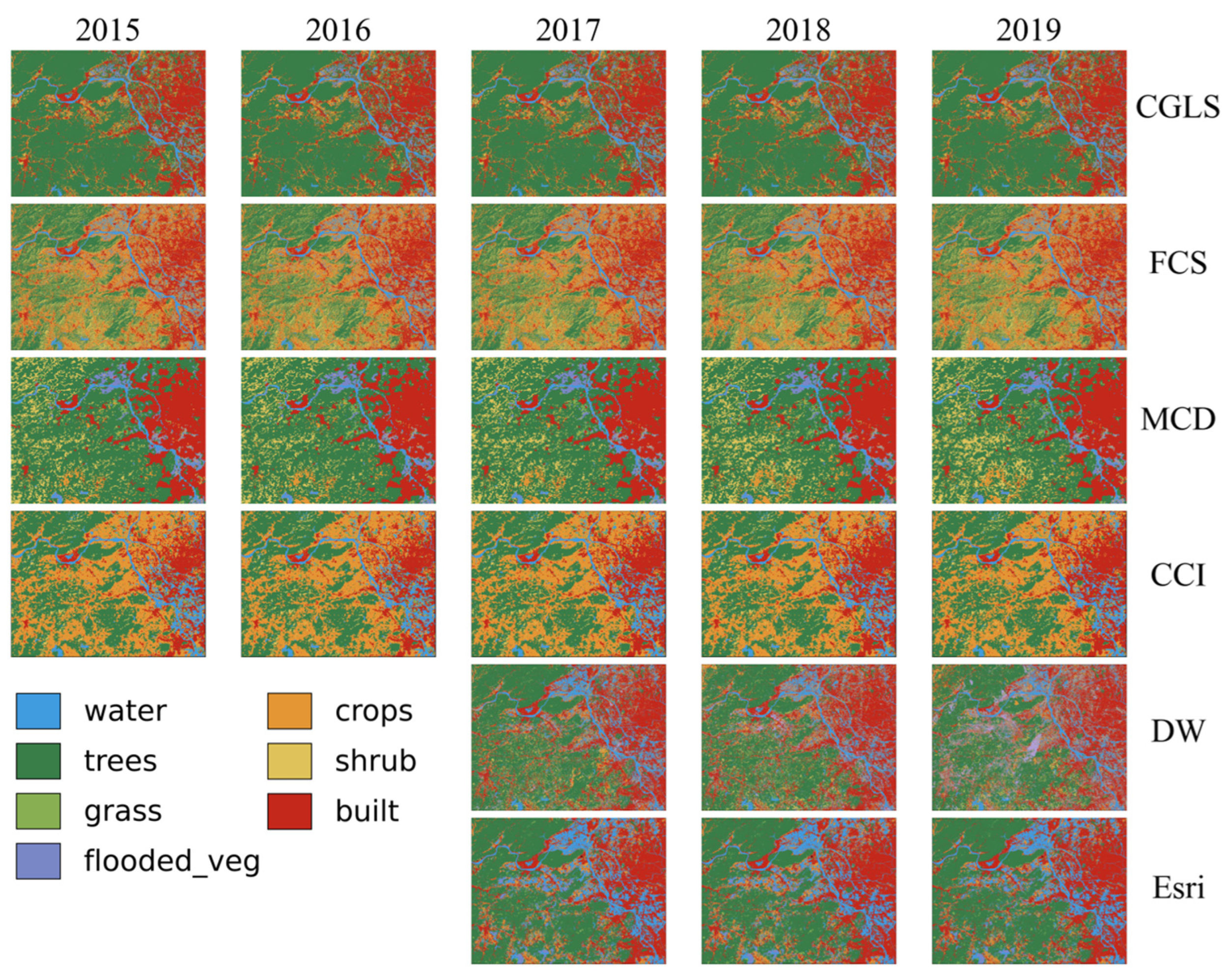
The central portion of the GHMA is distinguished by its high urbanization rate and diverse land cover types (
Figure 2). Between 2015 and 2019, the central urban area experienced significant expansion, with large tracts of cropland and low-density vegetation being replaced by urban land.
In the Visalia region of the United States, the landscape is predominantly agrarian, characterized by vast farmlands (
Figure 3).
Between 2015 and 2019, the area of farmland remained relatively stable and also showed a downward trend, reflecting changes in agricultural practices and land management policies.
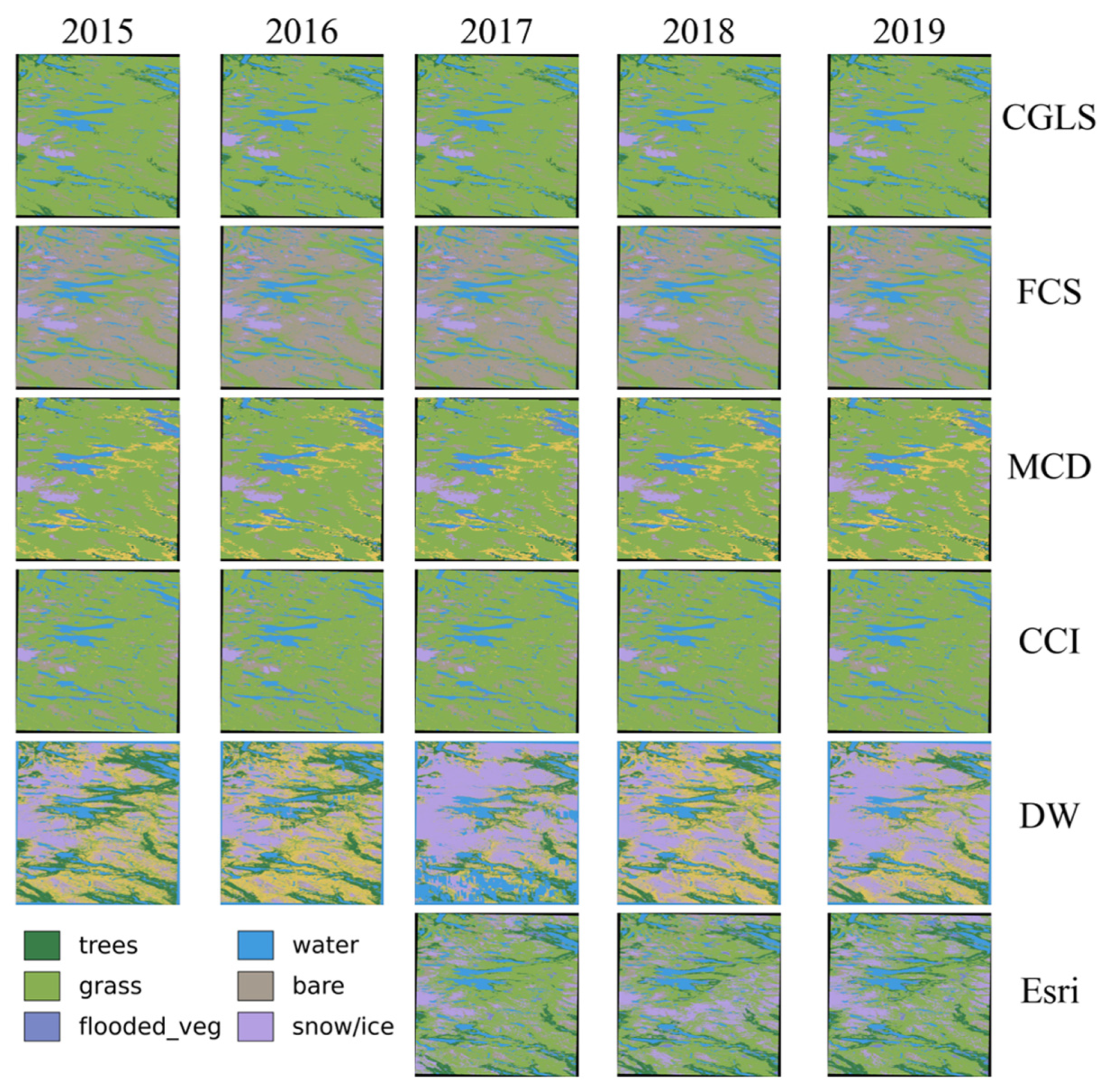
The central part of the Norwegian–Swedish border is located in the high latitudes of the northern hemisphere and is predominantly covered by forests (dark green), with scattered grasslands (light green) and shrubs (yellow), resulting in a high overall vegetation cover (
Figure 4).
Between 2015 and 2019, forest area remained stable, while grassland and shrub areas increased in some mountainous regions, reflecting the effects of climate warming and the natural recovery of vegetation.
Regional land cover exhibits spatial consistency but also significant differences across datasets. The CGLS dataset demonstrates consistent performance with minimal variation, particularly in forest and water body classifications. In contrast, the FCS and MCD datasets show greater fluctuations in arable and grassland classifications. The CCI dataset struggles to clearly distinguish between shrubs and grasses, leading to overlapping classifications in some regions. MCD is more accurate in classifying urban areas and bare land. The DW dataset stands out for its refined classification capabilities, especially in urban and bare land identification.
The classification of floodplain vegetation near water bodies varies across products. CGLS and Esri show greater sensitivity to floodplain vegetation, while FCS and MCD tend to misclassify portions of the floodplain as grassland or shrubs. For built-up areas, DW demonstrates a notable increase between 2017 and 2019, capturing urban sprawl with higher precision. These findings highlight the importance of selecting appropriate datasets based on specific research objectives and regional characteristics.
4.1. Classification Accuracy by Year
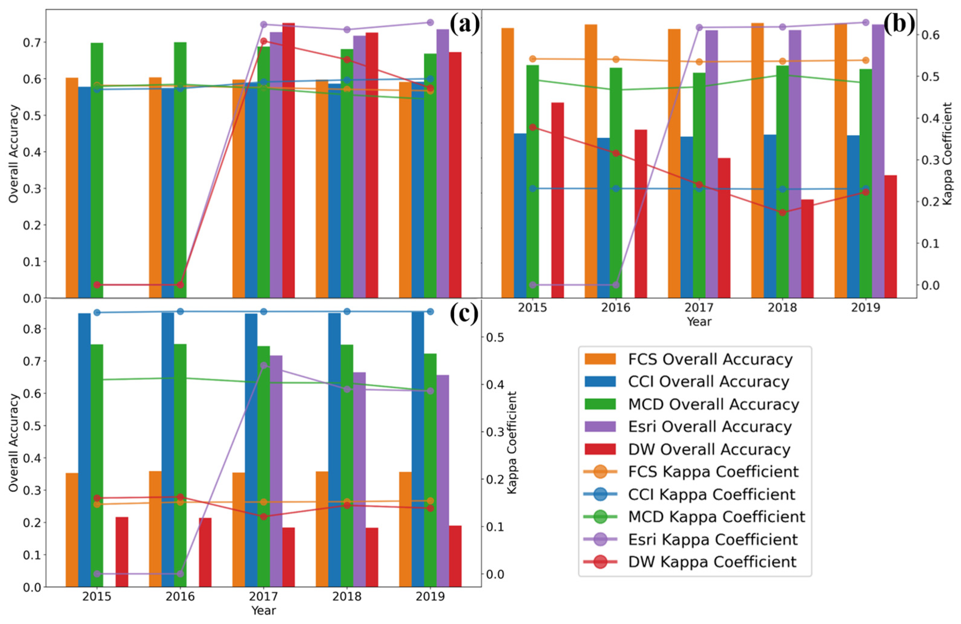
The classification accuracy of various products in the GHMA exhibited notable temporal variability between 2015 and 2019 (
Figure 5). The MCD products demonstrated higher accuracy in the initial years but experienced a decline in subsequent years. In contrast, Esri products showed significant fluctuations, with an initial rise in accuracy followed by a subsequent decrease. The DW products exhibited higher accuracy exclusively in 2017, with relatively lower accuracy in other years. On the other hand, FCS and CCI products maintained stable accuracy levels, achieving moderate overall performance throughout the study period. The Kappa coefficient exhibited a similar trend to the OA, underscoring the strong classification consistency and reliability of these products.
In Visalia, the accuracy of the products varied significantly across the study period, with certain products performing well in specific years while displaying large annual fluctuations. The DW product showed higher accuracy in certain years, while the FCS and CCI products were stable, although they did not exceed the peaks of other products. The fluctuating Kappa coefficients reflect the complexity of the land cover types in the region and the limited environmental adaptability of the products.
For the central part of the Norway–Sweden border, the accuracy of the products remained relatively stable without significant fluctuations. While some products exhibited higher or lower accuracy, the OA levels were consistent across the study period. The Kappa coefficients showed smaller variations, indicating that classification accuracy and consistency were more stable, though there was limited potential for performance improvement, likely constrained by local environmental factors.
The analysis highlights the varying performance of different classification products across regions and years. While some products demonstrated higher accuracy in specific areas, others maintained consistent performance. The Kappa coefficients further corroborate these findings, emphasizing the importance of selecting appropriate products based on regional characteristics and research objectives.
In terms of product performance, the accuracy of FCS is stable in both the GHMA and Visalia, but generally moderate overall. For the central Norway–Sweden border, the accuracy of FCS is influenced by topographic and climatic factors [
28,
29]. The accuracy of CCI remains relatively stable at a medium level, although the specific value varies by region. MCD exhibits higher accuracy in the early years, followed by a decline in the Greater Bay Area, while its performance in Visalia and the central Norway–Swedish border differs. In these regions, MCD’s accuracy shows smaller variations, reflecting its adaptability to environmental and land cover changes. The Esri product demonstrates more pronounced fluctuations in the Greater Bay Area, while its accuracy is more stable in the other two regions. The DW product shows exceptional performance in the GHMA and Visalia in certain years, but no such pattern is observed for the central part of the Norwegian–Swedish border.
4.2. Comparative Analysis of Different LULC Categories
This subsection compares the trends and causes behind the classification accuracy results of each product, based on the PA for each LULC category in the study area.
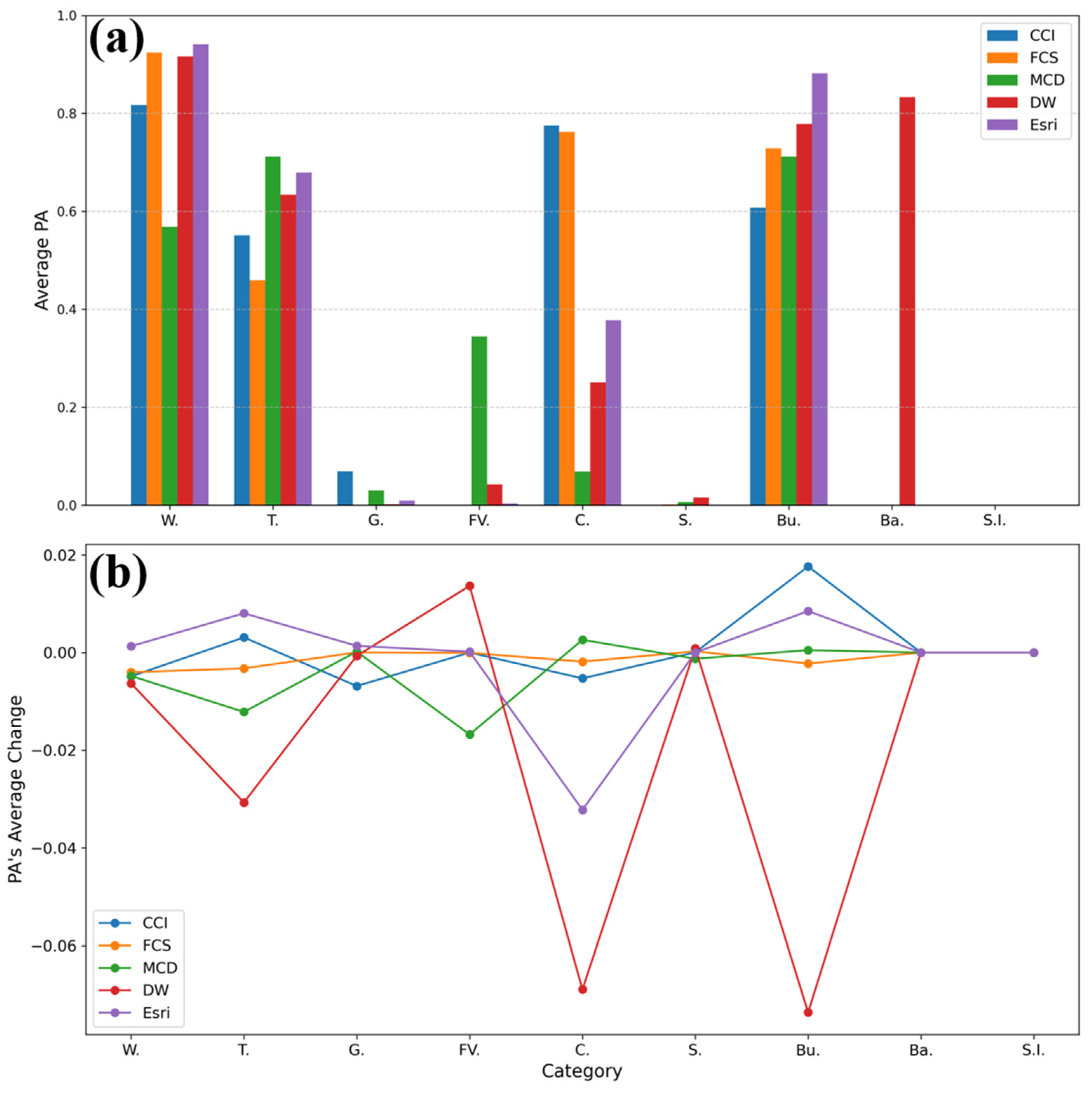
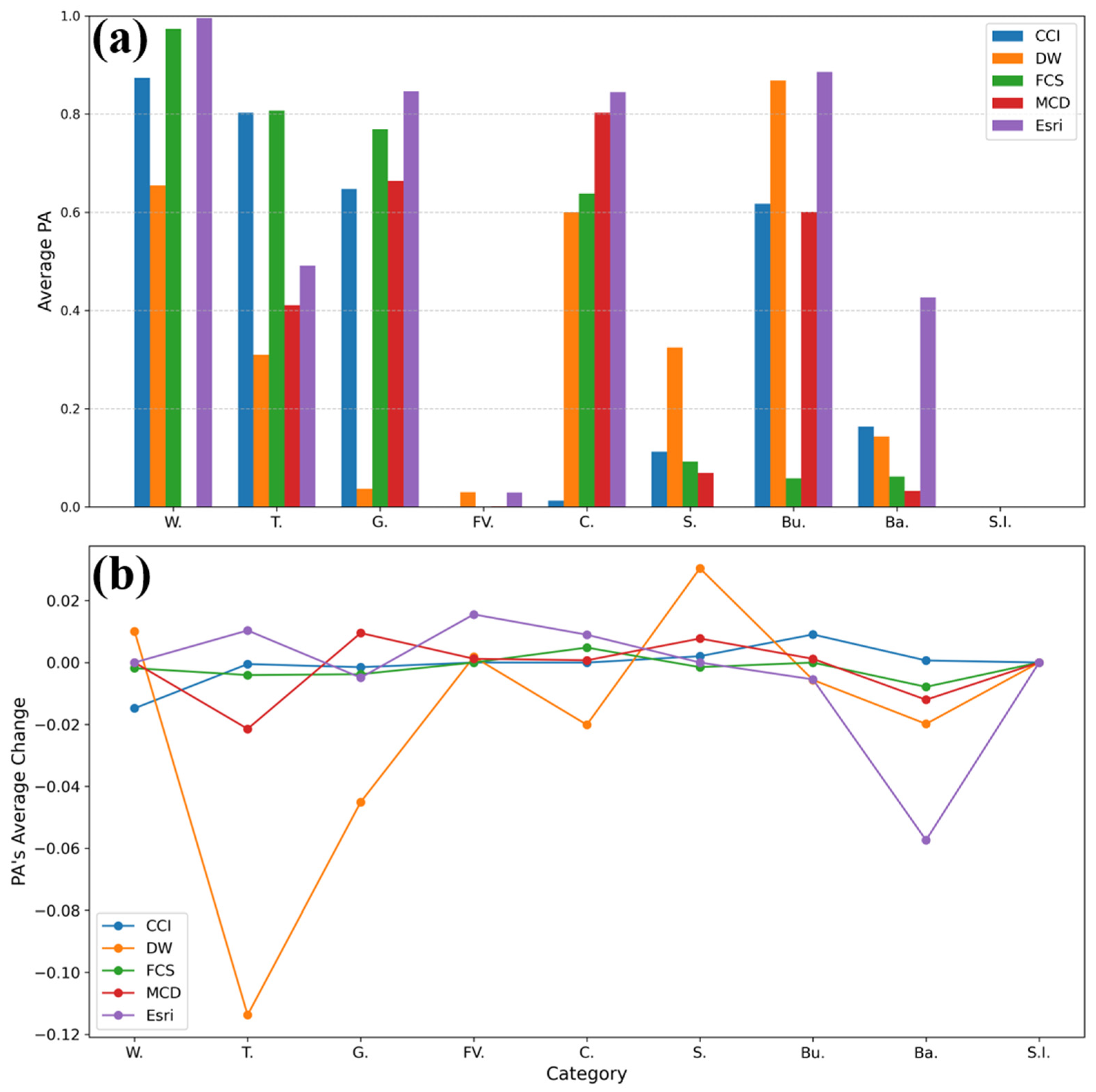
In the core region of the GHMA, where urban landscapes are interwoven with natural woodlands and complex topography, the PA of various land cover products exhibits substantial variability across LULC categories (
Figure 6). Analyzing classification accuracy from 2015 to 2019 reveals consistently high PA values for water, forest, and cropland, whereas grassland, bare ground, and shrubland demonstrate lower and more fluctuating accuracy levels.
Among the evaluated products, the CCI dataset consistently achieves high classification precision for water, with PA values exceeding 0.8, but exhibits challenges in accurately delineating grassland and bare ground. The DW product demonstrates superior performance in the cropland category, achieving near-perfect accuracy (PA ≈ 1) in 2019, highlighting its strong suitability for capturing specific land cover types in certain years. Similarly, the Esri product performs well in water classification, aligning closely with CCI. The FCS dataset initially exhibited high PA for water in 2015, but its accuracy progressively declined in subsequent years. Meanwhile, the MCD product maintains moderate classification accuracy for water. Overall, FCS and CCI demonstrate relatively stable performance across the GHMA, reflecting the robustness of their classification algorithms. However, the PA values for grassland, shrubland, and bare ground remain generally low, particularly in the DW and MCD products, with pronounced year-to-year fluctuations.
From a temporal perspective, classification accuracy remained relatively stable between 2015 and 2019, although some categories experienced notable shifts. CCI exhibited minimal variation, whereas FCS showed a gradual decline in water accuracy and a temporary improvement in grassland classification in 2017, followed by a subsequent drop. The DW product recorded a sharp surge in cropland accuracy in 2019 (PA ≈ 1), while MCD experienced a substantial decline in cropland accuracy in 2019 (PA ≈ 0.2). Despite these variations, classification accuracy for water remained consistently high across all products, underscoring the stability of its spectral characteristics, which facilitate reliable classification.
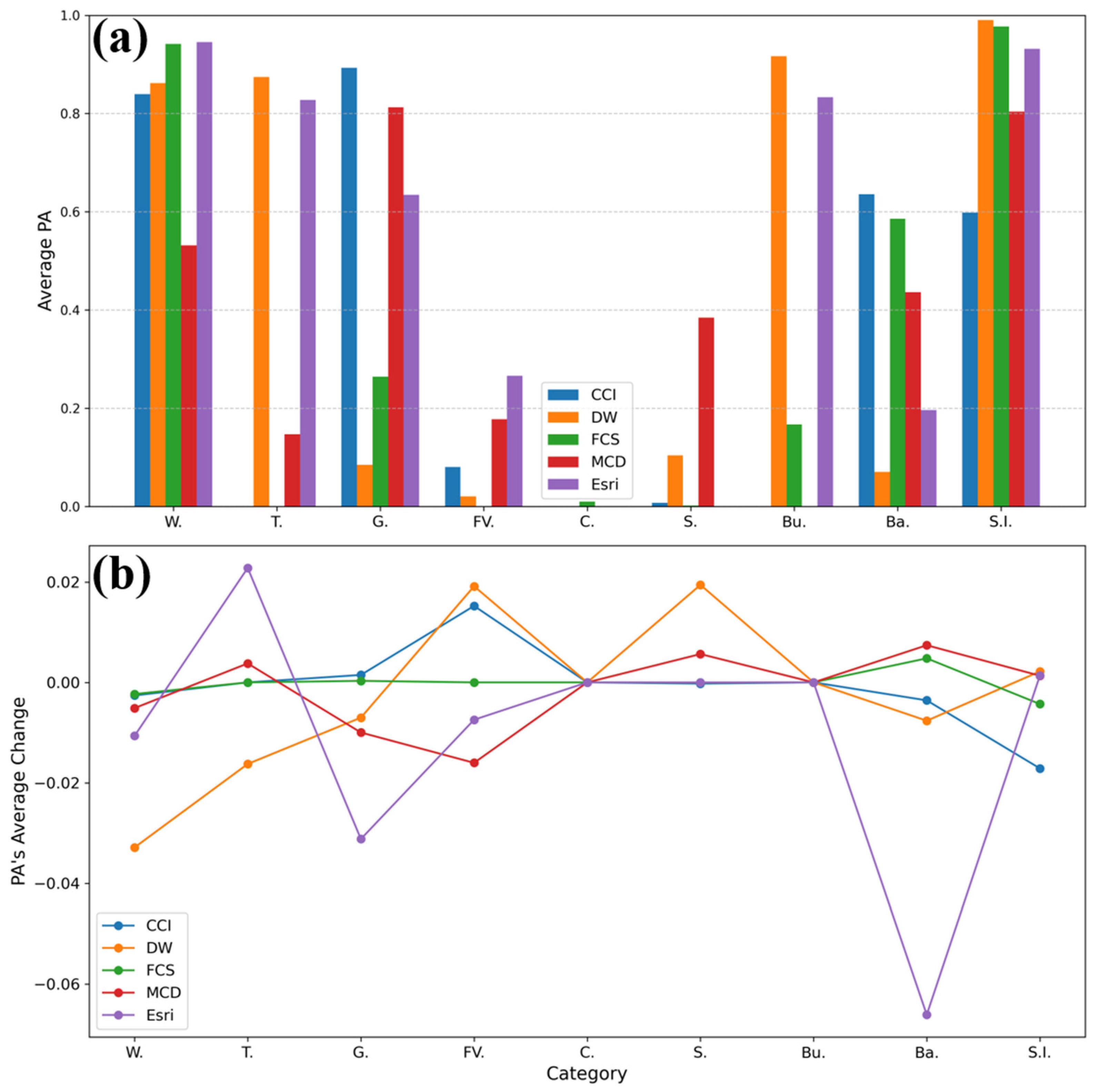
The Visalia region, situated at the interface of extensive cropland and natural landscapes, is characterized by diverse land cover types and significant anthropogenic influences. Analyzing classification accuracy trends from 2015 to 2019 reveals that most land cover products perform well in cropland and woodland classification, with the CCI dataset demonstrating consistently stable performance within a moderate-to-high accuracy range (
Figure 7).
Across the study period, the CCI product maintains stable accuracy levels, reinforcing its reliability in land cover classification. The DW product exhibits strong performance, particularly in 2019, when cropland classification accuracy approaches 1, indicating its effectiveness for specific years. Similarly, the Esri product maintains high and stable accuracy across multiple categories, suggesting robust classification capabilities. The FCS dataset performs well, particularly in the tree and grass (likely representing impervious surfaces or built-up areas) categories. Conversely, the MCD product, while achieving moderate accuracy in water classification, demonstrates significant fluctuations in grassland and cropland, indicating variable monitoring capabilities across different land cover types.
Accuracy variations are particularly pronounced among specific land cover categories. Water, trees, and built-up areas exhibit high and stable classification accuracy, suggesting that spectral consistency enhances the ability of these products to distinguish these classes. However, grassland and cropland categories show considerable accuracy fluctuations, likely influenced by complex spectral signatures, seasonal vegetation dynamics, and environmental variability, making them more challenging to classify with high consistency.
The time-series analysis further reveals that classification accuracy in the Visalia region remains relatively stable over time, with CCI and FCS displaying smooth year-to-year variations. However, DW exhibits significant fluctuations, particularly in the tree category, where accuracy is highly unstable, suggesting that DW may not be well suited for dynamic tree cover classification. Conversely, classification accuracy for the built-up category remains consistently high across products, highlighting their effectiveness in monitoring urban expansion. Nonetheless, classification performance for other land cover categories showed a decline over time, reflecting ongoing challenges in accurately capturing complex landscape dynamics.
The central Norwegian–Swedish border region, characterized by high-latitude woodlands with complex land cover features and strong climatic influences, exhibits generally high classification accuracy in the snow and ice and grassland categories from 2015 to 2019 (
Figure 8).
Among the evaluated products, CCI demonstrates superior PA in water and tree classifications, while DW performs well across multiple categories, particularly in water. The Esri product maintains consistently high accuracy in the water and tree categories, indicating stable classification performance over multiple years. The FCS product exhibits strong accuracy in water classification but shows fluctuating performance in other categories, suggesting variability in its adaptability to different land cover types. Meanwhile, the MCD product maintains a moderate level of accuracy across categories.
Significant accuracy variations are observed across land cover categories. Most products achieve high and stable classification accuracy in water, reflecting the spectral distinctiveness of this category. However, grassland and cropland classifications display greater fluctuations, with noticeable accuracy variations across different products, likely due to seasonal vegetation changes and spectral mixing.
From a temporal perspective, classification performance remains relatively stable across products, with year-to-year accuracy changes generally within ±0.07. FCS exhibits the most stable performance, while the Esri product shows relatively larger fluctuations over time. Despite these variations, overall classification stability is high in this region, although the Esri product appears less effective in capturing wasteland features.
4.3. Annual Temporal Accuracy
This section evaluates temporal accuracy, as defined in
Section 3.2.2, to assess each product’s ability to detect and track land cover changes over time.
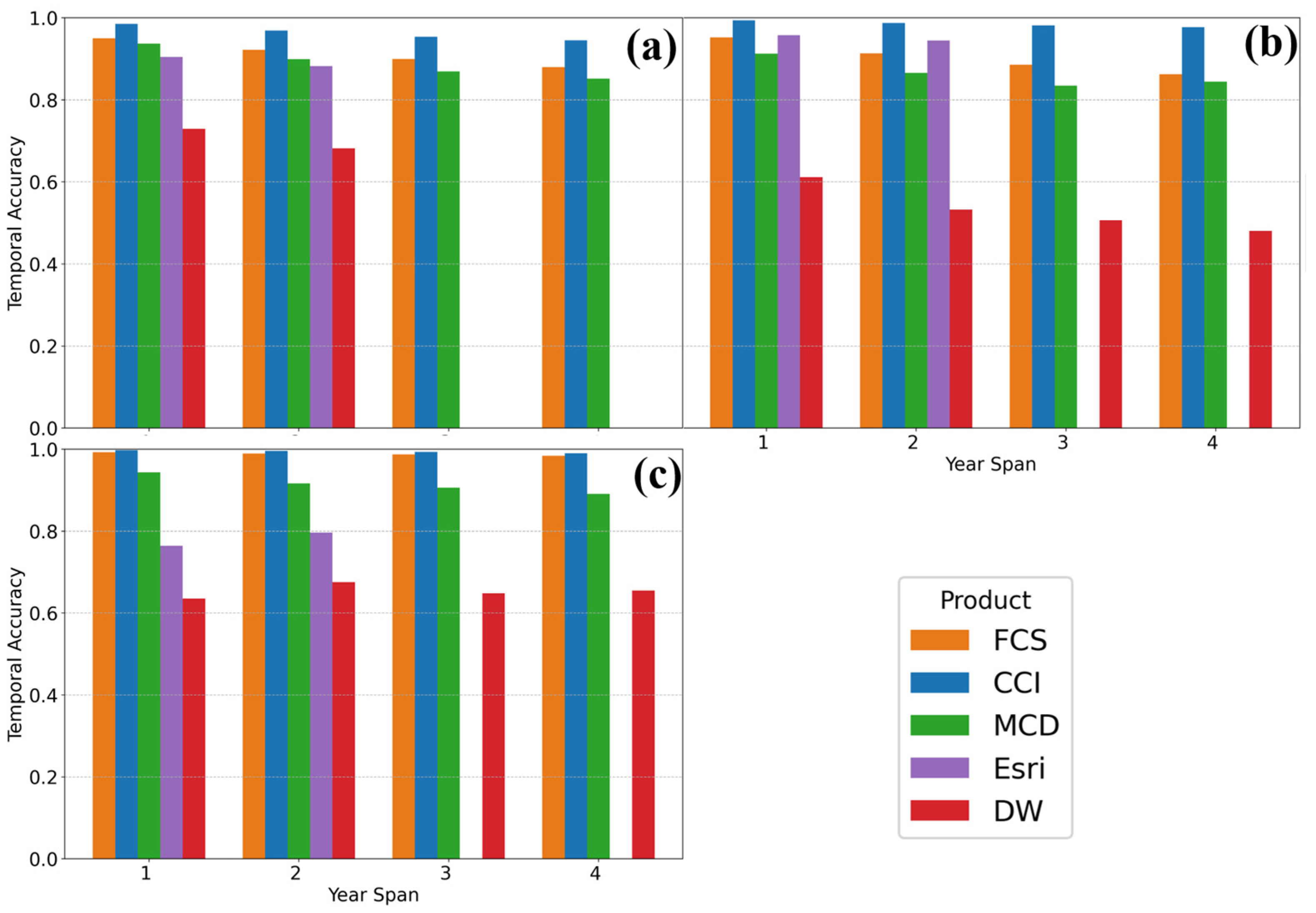
Figure 9a presents the accuracy of dynamic land cover changes across different time spans for each product in the GHMA. FCS and CCI exhibit the highest accuracy for shorter time spans, indicating their strong capability for high-frequency land cover monitoring. Their ability to capture rapid landscape transitions makes them particularly effective in this region. Conversely, DW consistently exhibits the lowest accuracy across all time spans, suggesting weaker performance in detecting dynamic land cover changes. Esri and MCD demonstrate intermediate accuracy, with notable fluctuations, though they achieve comparable performance to FCS and CCI under certain conditions.
In Visalia, USA, FCS maintains high accuracy and stable performance across all time spans, highlighting its adaptability and reliability in monitoring land cover changes. CCI performs well over shorter time spans but experiences a notable accuracy decline as the time span increases, indicating reduced effectiveness for long-term monitoring. Esri outperforms other products for medium-length time spans, exhibiting stable accuracy and robust performance in capturing land cover transitions. MCD remains relatively stable with moderate accuracy, while DW continues to underperform across all time spans, failing to achieve reliable accuracy in any period.
In the central Norwegian–Swedish border region, FCS and CCI products exhibit strong accuracy for shorter time spans but show significant declines in performance over longer periods, making them less suitable for long-term monitoring. Esri, however, maintains a consistent accuracy level across all time spans, demonstrating stability despite not excelling in any particular period. This suggests that Esri is more reliable for long-term monitoring in this region. MCD remains stable with moderate accuracy, exhibiting fewer fluctuations than other products. DW, once again, records the lowest accuracy across all time spans, reinforcing its limited capacity for tracking land cover dynamics in this region.
Across all three study regions, FCS consistently delivers high accuracy in tracking dynamic land cover changes, particularly over shorter time spans, underscoring its versatility and adaptability to diverse monitoring needs. CCI excels in short-term monitoring in the GHMA and Visalia but demonstrates weaker performance in the Norwegian–Swedish border region, suggesting regional variability in its effectiveness. Esri exhibits notable performance variation, excelling in the 2-year time span in Visalia, where it outperforms other products in land cover change detection. MCD maintains a stable, moderate accuracy across all regions, yet lacks exceptional performance in any specific scenario. Finally, DW consistently underperforms in all three regions, with low accuracy across all time spans, highlighting its limitations in capturing land cover change dynamics.
5. Discussion
In
Section 4, we presented the results of a comprehensive quantitative analysis of six global time-series land cover data products, assessing their annual classification accuracy, classification performance for different LULC categories, and annual temporal accuracy in three distinct study areas. These analyses revealed the strengths and limitations of each data product under various environmental conditions and LULC types. In this section, these land cover changes will be visually interpreted and discussed together with the results of
Section 4 to provide a more intuitive understanding of the actual meaning behind the data and to further explore the applicability of each data product in practical applications.
Considering the rapid urban expansion and diverse LULC types in the GHMA, the FCS, CCI, and DW datasets are suitable choices for monitoring urban expansion and land cover changes. The high resolution (30 m) and refined classification system of FCS effectively identify the details of urban expansion, the long-term data (1992–2024) of CCI are suitable for analyzing long-term trends in urban expansion, and the near-real-time data of DW can monitor the dynamic changes of urban expansion in a timely manner.
In the Visalia region, where land cover types include croplands, grasslands, and urban areas, the MCD and Esri datasets are effective for monitoring urban expansion and land cover changes. MCD provides long-term data (2001–2024) and moderate resolution (500 m), which are suitable for analyzing long-term trends and regional changes in urban expansion, while Esri’s high resolution (10 m) and deep learning technology effectively identify different LULC types, thus accurately monitoring urban expansion.
In the Norway–Sweden border area, dominated by forests and grasslands, the FCS and CCI datasets are effective for monitoring urban expansion and land cover changes. The high resolution (30 m) and refined classification system of FCS can effectively identify forest and grassland types, while the long-term data (1992–2024) of CCI are suitable for analyzing the impact of climate change on forests and grasslands, thereby indirectly monitoring the ecological impact of urban expansion.
5.1. Classification Criteria
A commonality exists among the classification systems of various land cover products, as they all encompass major land cover types. This similarity enables the comparative analysis of classification performance and temporal variations across products within broadly aligned categories. However, it should be noted that there are also significant differences in category definitions and the degree of subdivision across these systems [
30]. For instance, the FCS product differentiates multiple subtypes within the “water” category, including swamp, marsh, flooded flat, and water body, whereas the CCI product consolidates all these subtypes into a single water category. Such discrepancies can lead to classification mismatches, where the same land feature is assigned to different categories across products or where a category encompasses heterogeneous land types. These variations directly impact the reliability of time-series comparisons and trend analyses.
The three-level mapping strategy demonstrates robust performance in categories with pronounced spectral distinctiveness or clearly defined criteria. However, when handling classes with spectral–temporal feature overlap (e.g., grassland/cropland), its effectiveness can be influenced by source data resolution and regional heterogeneity. This limitation is further exemplified by contrasting classification outcomes across regions. In the Norway–Sweden border area, consistently high bare land accuracy reflects the strategy’s strength in distinguishing spectrally distinct features with minimal environmental complexity. Conversely, lower shrubland classification accuracy in the GHMA underscores challenges in resolving mixed vegetation classes within heterogeneous landscapes, where spectral ambiguity and sparse validation data exacerbate mapping uncertainties. Future enhancements should focus on integrating multimodal data and automated rule-based frameworks to improve the strategy’s generalizability and objectivity.
Beyond classification criteria, the mapping process itself affects analysis reliability. The accuracy of category mapping directly influences the reliability of temporal land cover change analyses across multi-source datasets. Misclassification during mapping can introduce two key issues. The first issue is a spatial mismatching problem. For example, misclassifying grass as trees leads to the conclusion of “false forest expansion” [
31]. The second one is that of time-series distortion. The process of vegetation gradual change is characterized as abrupt or static in different products due to differences in classification criteria, which interferes with trend analysis. For example, vegetation succession in a region shows gradual change in FCS due to classification refinement, while it shows stability in CGLS due to broad categories, leading to contradictory trends across products. Therefore, when analyzing trends in temporal changes, it is necessary to fully consider the effects of classification mapping and interpret differences and changes between products with caution.
When analyzing temporal land cover trends, it is crucial to account for classification mapping effects and interpret inter-product differences cautiously. A robust mapping framework, combining direct category alignment, spectral feature integration, and expert validation, mitigates misclassification risks and improves the reliability of land cover change assessments.
5.2. Precision Calculation
In land use and land cover time-series change analysis, resampling to a consistent spatial resolution can enhance cross-product monitoring capacity comparisons. However, this process may also introduce accuracy index bias due to spatial distribution distortions and area mismatches [
32].
Integrated accuracy evaluation is crucial in land cover studies to ensure the reliability of study results. For classification accuracy, this study employed a randomized 50% window sampling method, averaging results over three iterations, in combination with a fixed 5 × 5 window strategy. This approach helps mitigate spatial heterogeneity and random noise interference. However, fixed-window sampling may overlook large-scale feature characteristics and mask localized land cover changes, potentially smoothing evaluation results and reducing sensitivity to small-scale variations [
33]. For time-series accuracy, this study utilized a year-by-year comparison approach to assess the consistency of land cover changes across different time scales. This method reveals the long-term performance of classification models through cross-year spanning analysis. However, the use of a 20% random sample size may be insufficient in certain cases, and spatial distribution biases can introduce assessment uncertainty, particularly in spectrally complex regions where classification errors are more likely.
Despite its effectiveness, the current evaluation method has several limitations. The fixed-window approach struggles to balance feature-scale differences. Small windows are susceptible to mixed-pixel effects, while large windows reduce sensitivity to local changes and can obscure finer-scale land cover dynamics. Reliance on a single validation source may lead to spatiotemporal mismatches, affecting the reliability of accuracy assessments. Gradual transitions and mixed-type changes in land cover increase the difficulty of time-series matching, making it challenging to capture nuanced temporal variations.
Therefore, in order to improve the accuracy evaluation, we can improve the following three aspects:
- (1)
Dynamic sampling optimization with adaptive window design based on land class spatial heterogeneity and stratified sampling to proportionally allocate samples by type, thereby improving representativeness.
- (2)
Multi-source data fusion validation by integrating high-resolution imagery, UAV data, and field surveys to construct a spatiotemporally synchronized reference database, thereby reducing validation bias [
34].
- (3)
Error-driven parsing and algorithm enhancement by quantifying dominant error sources such as spectral confusion and terrain effects [
35,
36], and optimizing temporal correlation modeling and change detection mechanisms to enhance the monitoring robustness of gradual processes and mixed land classes.
5.3. Differences in the Products
In the analysis of changes within specific land cover categories, significant variations were observed in the performance of different products across the three study regions: the GHMA, the Visalia region, and the Norway–Sweden border. No single product consistently demonstrated an absolute advantage across all land categories and regions, highlighting the complexity of classification accuracy in diverse environments. The following sections detail the specific differences and their implications.
5.3.1. Environmental and Anthropogenic Influences
In economically developed regions like the GHMA, highly dynamic land cover changes can lead to update lag errors in classification products. The rapid transformation of urban landscapes places higher demands on time-sensitive monitoring [
37]. For instance, in the GHMA, products like FCS with high spatial resolution (30 m) are better suited to capture the rapid urban expansion, while DW’s near-real-time data help in monitoring the most recent changes. Fluctuations in climate conditions further complicate classification, particularly in grasslands, wetlands, and water bodies, as they influence vegetation phenology rhythms and alter area dynamics, leading to reduced classification consistency [
38,
39], especially for products like CCI which rely on longer time-series data.
5.3.2. Impact of Data Sources and Sensor Resolution
Differences in data sources, sensor types, and spatial resolution directly impact classification accuracy. Products based on high-resolution satellite imagery, such as FCS (30 m) and DW (10 m), perform well in categories with large, homogeneous areas and distinct spectral signatures (e.g., water bodies). However, they struggle with complex spectral features found in fragmented landscapes such as grasslands. For example, in the Norway–Sweden border region, the classification of grasslands and forests using FCS can be challenging due to mixed pixels. Low-frequency data updates can result in outdated images, failing to capture sudden land cover changes, which has been a challenge in water body detection for products like CCI that have medium spatial resolution (300 m) and may not capture the most recent changes in dynamic regions [
40].
5.3.3. Limitations of Classification Algorithms
Traditional classification methods often lack sensitivity to spectral confusion and environmental variations in complex land cover categories, limiting their generalization ability. While deep learning models like those used in DW have demonstrated robust performance in homogeneous environments, they still exhibit biases in boundary recognition, particularly in fragmented urban landscapes such as bare ground patches [
41]. For example, in the Visalia region, products like MCD may struggle with accurately delineating boundaries between cropland and grassland due to similar spectral characteristics.
To enhance classification robustness in complex environments, future research should focus on the following improvements:
- (1)
The Integration of Multi-Source Remote Sensing Data: Combine optical, radar, and LiDAR data to improve the detection of diverse land cover types under varying environmental conditions. Develop adaptive classification frameworks that incorporate local land cover characteristics. For example, in the GHMA, urban expansion patterns can be better captured by integrating high-resolution optical and radar data to account for frequent cloud cover and rapid changes. Products like FCS and CCI can benefit from such integration to improve their accuracy in complex urban and forested areas.
- (2)
Real-Time Monitoring and Validation: Integrate Unmanned Aerial Vehicles (UAVs) and ground sensor networks to create an air–sky–ground calibration platform. This system would enable the real-time detection of surface changes, helping to reduce update lag errors in time-series monitoring, especially in dynamic regions like the GHMA where urban expansion is rapid. DW’s near-real-time data can be further enhanced through such a platform to provide more accurate and timely updates.
- (3)
Advanced Algorithm Development: Improve deep learning-based classification models by enhancing their ability to differentiate between spectrally similar land cover types and accurately delineate boundaries in heterogeneous landscapes. Develop hybrid models that incorporate physical-based and data-driven approaches to improve classification stability and accuracy, particularly in regions with complex land cover such as the Norway–Sweden border. For instance, combining the strengths of FCS’s high resolution with advanced algorithms could lead to the better classification of forest and grassland boundaries in this region.
6. Conclusions
This study undertakes a comprehensive analysis of six recent time-series land cover datasets, incorporating the critical metric of time-series accuracy to evaluate their performance across three representative regions. The evaluation framework integrates both classification accuracy and time-series accuracy assessments, enabling a robust and systematic comparison of multi-source, long-time-series land cover data.
The comparison results indicate that while the datasets exhibit spatial consistency, significant discrepancies exist in land cover classification. In terms of accuracy performance, each dataset demonstrates varying levels of accuracy depending on the region and land cover type, with no single dataset outperforming others in all case study areas. FCS is good for short-term forest and urban expansion monitoring due to its high versatility and stability in short-term dynamic changes, but needs improvement in long-term monitoring and complex land cover identification. CCI is characterized by long-term continuity, medium resolution, and stable classification accuracy, and is suitable for scenarios requiring long-term land cover change analysis (e.g., climate modeling, ecological trend studies), but in complex terrain or fragmented land cover areas, it needs to be combined with high-resolution data to improve accuracy. Esri is recommended for high-resolution analysis in specific regions like urban planning and agricultural areas due to its excellent performance in certain time spans and regions, but has limited adaptability elsewhere. MCD maintains moderate accuracy across regions, suitable for medium-resolution regional land cover analysis. DW, while generally underperforming in dynamic land cover change monitoring, has some value in the preliminary monitoring of rapidly changing areas due to its near-real-time data. For dataset selection, with reference to the regional context, the following recommendations are made:
In the GHMA, FCS, CCI, and DW are recommended. FCS’s high resolution (30 m) and detailed classification system effectively capture urban expansion details. CCI’s long-term data are suitable for analyzing long-term trends. DW’s near-real-time data can monitor urban expansion dynamics in a timely manner.
In the Visalia region of the United States, MCD and Esri are suggested. MCD’s long-term data and medium resolution are good for analyzing long-term trends and regional changes. Esri’s high resolution and deep learning technology effectively identify different land cover types.
In the Norway–Sweden border region, FCS and CCI are recommended. FCS’s high resolution and detailed classification system effectively identify forest and grassland types. CCI’s long-term data and medium resolution are suitable for analyzing long-term trends and the impact of climate change.
While the recommendations above are derived from rigorous analysis across three diverse transitional regions, we recognize that their applicability to other global contexts (e.g., arid zones, tropical rainforests, or small island states) may vary. These case studies provide a foundation for context-driven dataset selection but do not fully capture the complexity of all landscapes. We therefore encourage future research to expand validation efforts to underrepresented regions, such as sub-Saharan Africa, the Amazon Basin, or the Tibetan Plateau, to further refine and generalize these findings. Such work would strengthen the global applicability of land cover dataset selection strategies and address remaining gaps in heterogeneous environments.
While contemporary land cover products provide valuable insights for long-term monitoring, they face three critical constraints: semantic inconsistencies in class definitions, identification errors across complex land surfaces, and limited sensitivity to transitional dynamics. To address these challenges, next-generation data development requires standardized hierarchical taxonomies with ecoregion-adapted ontologies to ensure multi-scale representational fidelity. Concurrent technological integration should combine multi-sensor synergies (optical/SAR/LiDAR), implement physics-constrained super-resolution architectures for temporal coherence, and embed process-aware mechanisms through coupled land–atmosphere modeling. This integrated approach targets enhanced spatiotemporal continuity and classification logic integrity across heterogeneous landscapes, particularly improving transitional zone characterization and change detection reliability in peri-urban/ecotone regions.


 ,
, 

