Article

Temporal Denoising of Infrared Images via Total Variation and Low-Rank Bidirectional Twisted Tensor Decomposition

MOE Key Laboratory of Optoelectronic Imaging Technology and System, Beijing Institute of Technology, Beijing 100081, China
*
Author to whom correspondence should be addressed.
Remote Sens. 2025, 17(8), 1343; https://doi.org/10.3390/rs17081343
Submission received: 21 February 2025 / Revised: 22 March 2025 / Accepted: 23 March 2025 / Published: 9 April 2025
(This article belongs to the Special Issue Recent Advances in Infrared Target Detection)

Abstract

:
Temporal random noise (TRN) in uncooled infrared detectors significantly degrades image quality. Existing denoising techniques primarily address fixed-pattern noise (FPN) and do not effectively mitigate TRN. Therefore, a novel TRN denoising approach based on total variation regularization and low-rank tensor decomposition is proposed. This method effectively suppresses temporal noise by introducing twisted tensors in both horizontal and vertical directions while preserving spatial information in diverse orientations to protect image details and textures. Additionally, the Laplacian operator-based bidirectional twisted tensor truncated nuclear norm (bt-LPTNN), is proposed, which is a norm that automatically assigns weights to different singular values based on their importance. Furthermore, a weighted spatiotemporal total variation regularization method for nonconvex tensor approximation is employed to preserve scene details. To recover spatial domain information lost during tensor estimation, robust principal component analysis is employed, and spatial information is extracted from the noise tensor. The proposed model, bt-LPTVTD, is solved using an augmented Lagrange multiplier algorithm, which outperforms several state-of-the-art algorithms. Compared to some of the latest algorithms, bt-LPTVTD demonstrates improvements across all evaluation metrics. Extensive experiments conducted using complex scenes underscore the strong adaptability and robustness of our algorithm.

Graphical Abstract

1. Introduction

Infrared focal plane arrays (IRFPAs) are extensively used in the defense, medical, industrial, and security fields [1,2,3]. Specifically, they play a crucial role in applications such as target detection and tracking (especially in remote sensing scenarios where atmospheric turbulence and sensor limitations introduce significant noise), situational awareness, non-destructive testing, and medical diagnosis [4,5,6]. Moreover, IRFPAs are vital for surveillance under low-light or adverse weather conditions, where noise levels are often higher, impacting the visibility of small targets [7]. Point target detection in IRFPA imaging faces several challenges. Key among these are two linearly independent interferences, random unstructured noise and structured background clutter. While noise appears as random fluctuations, clutter manifests as structured patterns from complex background scenes that may be mistaken for targets. In addition to these, the inherent characteristics of IRFPA detectors introduce further complexities. The response of each unit in the detector array is inconsistent and unstable [8,9]. This is due to factors such as the detector material characteristics, manufacturing processes, and optical systems. This inconsistency leads to the superimposition of spatial fixed-pattern noise (FPN) and temporal random noise (TRN) on the scene image. FPN manifests as a consistent spatial pattern, while TRN varies randomly over time. Background clutter, on the other hand, arises from the complexity and variability of the scene itself. This issue is particularly prominent for uncooled IRFPA, which has low sensitivity and is more susceptible to FPN and TRN, significantly affecting the imaging quality [10]. This is especially relevant for surveillance applications using low-cost, uncooled infrared detectors, which are generally more susceptible to noise than cooled ones [11,12]. In practical applications, TRN can significantly degrade the performance of IRFPA systems. For instance, it can reduce the signal-to-noise ratio and contrast of the image, mask the detailed information of the target, and introduce false alarms and missed detections, thereby reducing the reliability of target detection and tracking. In practical applications, TRN can markedly diminish the performance of IRFPA systems by reducing the image’s signal-to-noise ratio and contrast, obscuring detailed target information, and leading to false alarms and missed detections. This paper focuses on addressing the challenge of TRN suppression in infrared small target detection, recognizing its significant impact on system performance.
Image denoising is an important step in object recognition tasks. It offers several benefits, including improved accuracy and recall rate, enhanced adaptability to complex environments, and increased algorithm robustness [13,14,15]. This ultimately leads to more stable and reliable detection systems. Furthermore, in the context of infrared imaging, effective denoising is critical for enhancing the performance of various applications. For example, in target detection and tracking, denoising can improve the detection range and accuracy, especially for small or low-contrast targets. In addition, our proposed denoising method can serve as a preprocessing step to improve the input and enhance the performance of existing target tracking algorithms [16,17,18]. In situational awareness, denoising can enhance the clarity and interpretability of infrared images, leading to better understanding of the environment. In non-destructive testing and medical diagnosis, denoising can improve the sensitivity and reliability of defect or disease detection. The denoising process can be performed separately from the object recognition task or completed simultaneously as a whole. For deep learning-based object recognition methods, networks with deeper layers have good feature extraction capabilities, and specifically designing a denoising step may lead to limited improvement in recognition accuracy and affect computational efficiency [19]. For most object recognition methods, the impact of dataset quality is more obvious, and denoising preprocessing can effectively improve recognition accuracy [20,21,22,23].
FPN generally manifests as fixed patterns in the spatial domain, and relatively good correction effects can be achieved through methods such as calibration or scene-based approaches [24,25,26,27]. While background clutter can be mitigated through sophisticated background estimation and subtraction techniques, the TRN in IRFPAs predominantly appears as horizontal and vertical stripe noise [10]. Although often approached as spatial noise, standard IRFPA calibration techniques for stripe noise, be it FPN or TRN, typically depend on single-frame data. This approach neglects the potential benefits of exploiting temporal correlation. While the significance of temporal noise has been acknowledged [28], subsequent research [29] underscores the need for developing calibration methods that effectively leverage inter-frame relationships. While research on TRN suppression in infrared imagery is still developing and offers a limited number of dedicated methods, the field of video restoration boasts a wide array of established techniques, including temporal filtering, motion estimation, and motion compensation [30]. These methods, commonly employed in visible video denoising, leverage the temporal correlation in video sequences. This reliance on inter-frame relationships, prevalent in both video restoration and TRN reduction, supports the perspective that the denoising process for TRN can be fundamentally framed as a video restoration problem [31].
Deep learning-based methods are commonly used for visible video denoising [31,32,33,34,35,36,37], which also has reference significance for the infrared band. Although significant progress has been made using these methods, they generally involve the synchronized processing of multiple frames to maintain inter-frame correlation, resulting in high memory usage. The overall hardware costs for model training, deployment, and other aspects of noise reduction remain high [32,38]. Traditional video denoising methods are often developed from the field of image denoising [39,40], with some ability to resist detail blurring. However, there are issues to varying degrees, including blurred details, poor temporal consistency, extremely high computational complexity, and limited denoising effectiveness [39,41,42,43]. The denoising process utilizing tensor recovery methods is framed as a matrix or tensor recovery problem [44,45]. This approach employs techniques such as total variation and low-rank tensor decomposition for solving. Given that the inter-frame correlation is significant, this method shows great potential and has garnered considerable attention in recent years. However, the effectiveness of tensor recovery methods in video denoising, particularly regarding denoising performance and detail preservation, remains limited [46,47]. Additionally, when these tensor recovery methods are applied for TRN suppression in hyperspectral denoising, noticeable detail blurring occurs in moving targets [48,49]. Furthermore, the effectiveness of tensor recovery methods for TRN suppression in infrared small-target recognition is relatively weak [50,51].
Infrared target tracking heavily relies on temporal information between consecutive frames to accurately estimate the target’s motion trajectory [52,53]. However, traditional single-frame denoising methods ignore this crucial temporal correlation, limiting their performance. To better exploit this spatiotemporal information, we construct the image sequence into a three-dimensional tensor and propose a tensor decomposition-based denoising method. This paper proposes a TRN correction algorithm, named bidirectional twisted Laplacian and total-variation-regularized tensor decomposition (bt-LPTVTD), based on total variation and low-rank tensor decomposition, aiming to effectively correct infrared images affected by TRN. This method fully considers the correlation of temporal and spatial information. By employing advanced tensor decomposition techniques, the algorithm can both suppress noise and preserve crucial target motion information.
The remainder of this paper is organized as follows. Section 2 provides a brief overview of the representative tensor-decomposition-based image processing and denoising methods. Section 3 presents the notation and preliminary information related to tensor decomposition used in this paper. Section 4 describes the model and algorithm for the proposed bt-LPTVTD method. Section 5 presents the experimental analysis and results used to validate the proposed method. Finally, Section 6 highlights the major conclusions drawn from the findings of this study and directions for future research.

2. Related Works

Temporal denoising necessitates expanding the research focus from a two-dimensional matrix to a three-dimensional tensor to effectively leverage inter-frame correlation for improved denoising outcomes. TRN suppression methods can be classified into three categories: deep learning methods, traditional video denoising methods, and tensor recovery methods. The primary focus of tensor recovery methods is on developing tensor decomposition techniques and constructing tensor recovery models. Significant research has been conducted in the fields of hyperspectral image denoising and infrared small-target recognition in these areas [54], providing valuable insights for TRN suppression.

2.1. Deep Learning Methods

Deep learning-based temporal noise suppression methods are frequently applied to visible video denoising and can mainly be divided into two categories: convolutional neural network (CNN)-based methods and transformer-based methods. These models typically incorporate motion estimation or video frame alignment modules to strike a balance between effective denoising and the preservation of motion details.
In 2017, Zhang et al. [33] introduced a blind Gaussian denoising method utilizing a single deep convolutional neural network (CNN) for handling unknown noise levels. This method used residual learning to separate noise and included batch normalization to speed up the training process and improve denoising performance. In 2019, Claus et al. [55] developed Deep Blind Video Denoising (ViDeNN), which integrates spatial and temporal filtering within a CNN framework to achieve blind denoising while ensuring a degree of temporal consistency. Tassano et al. followed this with the Deep Video Denoising network (DVDnet) [34] and FastDVDnet [32] in 2019 and 2020, respectively. These approaches separate video noise into spatial and temporal components and employ two modules trained in two stages, resulting in enhanced denoising performance and significantly reduced computation time. In 2021, Sheth et al. [35] proposed an unsupervised deep video denoising (UDVD) method that trains exclusively on noisy data, achieving results comparable to those of supervised methods. In 2022, Monakhova et al. [56] leveraged generative adversarial networks (GANs) for video denoising in extremely low-light conditions. Additionally, Song et al. [37] introduced TempFormer, a hybrid model that combines temporal and spatial transformer blocks with three-dimensional convolutional layers to deliver high-quality video denoising. In 2024, Liang et al. [31] presented the Video Restoration Transformer (VRT) model, designed for tasks such as super-resolution, deblurring, denoising, frame interpolation, and spatiotemporal video super-resolution.
In recent years, deep learning-based video denoising methods have garnered significant attention and achieved remarkable advancements in denoising performance. However, these approaches have considerable memory requirements when processing image data, and video denoising methods that account for inter-frame correlations typically process multiple frames simultaneously, further increasing memory usage. As a result, the overall hardware costs for training, deployment, and related processes remain high. Moreover, deep learning methods often struggle to train effectively on real noisy images, and most denoising techniques are restricted to specific types of noise, limiting their applicability [57].

2.2. Traditional Video Denoising Methods

Traditional video denoising methods typically derive from image denoising techniques and frequently employ block-matching methods.
The traditional method for video denoising based on block matching is known as block-matching and 4D filtering (BM4D). This technique evolved from block-matching and 3D filtering (BM3D) and was introduced by Maggioni et al. [39,40] in 2012. Initially, BM4D was applied to denoise magnetic resonance images (MRI), but has since become commonly applied in video denoising. In 2014, Sutour et al. [41] presented a method for image and video denoising based on total variation, utilizing 3D blocks for spatiotemporal denoising. This approach integrated non-local means with total variation (TV) regularization, addressing the issues of high computational complexity and sensitivity to noise that are inherent in block-matching techniques. In 2018, Arias et al. [42] introduced a video denoising method grounded in empirical Bayesian estimation, which constructs a Bayesian model for each group of similar spatiotemporal blocks, thus mitigating issues arising from motion estimation inaccuracies. In 2019, Li et al. [43] achieved image and video recovery using a multi-plane autoregressive model combined with low-rank optimization.
In addition to block-matching methods, there are other approaches to video denoising that often incorporate block-matching techniques. In 2012, Reeja et al. [58] achieved video denoising by separating the background from the moving parts, applying temporal averaging and spatial filtering independently, which resulted in superior denoising performance compared to K-nearest filtering, while also fulfilling real-time processing requirements. In 2015, Han et al. [59] developed a nonlinear estimator for video denoising in the frequency domain, which simultaneously conducted motion estimation and noise observation, allowing for integration into video compression codecs to enhance computational efficiency. In the same year, Ponomaryov et al. [60] introduced a three-stage framework for denoising color video sequences affected by additive Gaussian noise, comprising spatial filtering, spatiotemporal filtering, and spatial post-processing. In 2020, Samantaray et al. [61] proposed a rapid trilateral filter for video denoising.
The 3D video denoising approaches of these traditional methods resemble those used for 2D images, as they consider temporal correlation through motion estimation techniques such as block matching. These approaches achieve video denoising with some resistance to detail blurring. However, due to the limited or costly utilization of inter-frame correlation, these methods often encounter issues such as detail blurring, poor temporal consistency, extremely high computational complexity, and limited effectiveness in denoising.

2.3. Tensor Recovery Methods

Tensor recovery methods consider image sequence blocks as the objects of processing and express them as matrix or tensor recovery problems, employing techniques such as total variation and low-rank tensor decomposition for their resolution. These methods effectively suppress temporal noise by operating jointly in the spatiotemporal domain, taking into account significant inter-frame correlations. As a result, they possess considerable potential and have garnered widespread attention in recent years.
Tensor recovery methods are applied in video restoration, where tensors consist of multiple temporally continuous images. These methods typically decompose the tensor into a recovery component and a noise component, with noise and interference characterized by the Frobenius norm, primarily focusing on recovery techniques. In 2017, Gui et al. [47] represented video 3D spatiotemporal blocks as a tensor structure and utilized low-rank tensor decomposition for denoising. This approach initially demonstrated the feasibility of tensor decomposition in video denoising. However, the simplicity of the tensor decomposition process makes it challenging to balance denoising and blur suppression. In the same year, Hu et al. [62] introduced a twisted tensor to optimize the tensor singular value decomposition (t-SVD) process by leveraging the temporal correlation of the video. They proposed the twisted tensor nuclear norm (t-TNN), which effectively preserves the details of moving objects. In 2022, Qiu et al. [63] introduced the tensor ring nuclear norm for estimating the recovery tensor, significantly enhancing computational efficiency. Additionally, Shen et al. [46] employed low-rank tensor decomposition to extract the background for foreground and background segmentation of noisy videos, using total variation to extract the foreground.
Beyond video restoration, tensor recovery methods have also found applications in hyperspectral image denoising and infrared small-target detection. In hyperspectral image denoising, methods like total variation regularized low-rank tensor decomposition [49], weighted norms combined with low-rank tensor decomposition [64], and variations of tensor nuclear norm [48,65,66] have been proposed to exploit spatial–spectral correlations and address mixed noise. For infrared small-target detection, tensor-based approaches often decompose the data into background, target, and noise components, with methods like asymmetric spatial–temporal total variation (ASTTV) regularization [51,67], truncated nuclear norm [68], and twisted tensor nuclear norm [50] being used to separate and recover the target of interest. However, many tensor-based video denoising methods are relatively simplistic, leading to limited effectiveness in noise reduction and detail preservation. For instance, while powerful in their domain, hyperspectral image denoising methods like LRTDTV [49] often struggle with temporal noise in videos, leading to blurred moving targets as they treat data as static sequences (Figure 1c). Similarly, infrared small-target recognition methods, such as ASTTV-NTLA [51], prioritize preserving dynamic targets but may compromise noise suppression, leading to a trade-off between denoising strength and detail preservation (Figure 1d,e). Therefore, achieving optimal results often requires careful parameter tuning, and further research is needed to develop more sophisticated tensor-based methods that can effectively address the challenges of temporal denoising in infrared image sequences.

3. Notations and Preliminaries

3.1. Notations

To ensure clarity in the subsequent sections, a detailed explanation of the symbols and theorems utilized in this study is provided beforehand. The symbols used in this study are listed in Table 1.

3.2. Anisotropic Spatiotemporal Total Variation Regularization

Because TV regularization preserves the spatial smoothness, edge structure, and spatial sparsity of images, it is widely used in image restoration, small-target recognition, and other fields [49,69,70,71,72]. However, most existing total variation denoising methods process only spatial 2D images, which can only describe the spatial characteristics of scene information and ignore the temporal changes in the target. If each image is separately subjected to spatial total variation denoising, it not only takes time but also ignores the smoothness characteristics of the scene in the temporal domain. Therefore, a more efficient total variation denoising method that can utilize the continuity of the target scene in both the spatial and temporal domains is required.
Owing to the strong correlation of scene information between consecutive frames and the smoothness exhibited in local spatial regions, asymmetric spatiotemporal total variation (ASTTV) can be used to simultaneously model the continuity of both space and time. ASTTV extends the 2D spatial TV to the 3D spatiotemporal domain, considering both the temporal and spatial total variations and combining them into a regularization term:
X A S T T V = D h X 1 + D v X 1 + δ D t X 1
where Dh, Dv, and Dt represent differential operators in the horizontal, vertical, and temporal dimensions, respectively. δ is a constant that controls the weighting of temporal differences. Dh, Dv, and Dt are defined as follows:
D h X ( i , j , k ) = X ( i + 1 , j , k ) X ( i , j , k )
D v X ( i , j , k ) = X ( i , j + 1 , k ) X ( i , j , k )
D t X ( i , j , k ) = X ( i , j , k + 1 ) X ( i , j , k )
The parameter δ assigns different weights to the time dimension TV and the space dimension TV, allowing for adjustments in the rate of change in the time dimension based on contextual information. We set δ = 0.5 following [73].

3.3. t-SVD and Rank Approximation Based on Laplace Operator

For the traditional tensor robust principal component analysis (TRPCA) model, convex relaxation methods are commonly used to solve traditional tensor robust principal component analysis models. Instead of minimizing the tensor rank, the tensor nuclear norms are minimized. The most commonly used method is t-SVD, which can be described as follows:
X = U S V T
Here, X R n 1 × n 2 × n 3 represents the original tensor. U R n 1 × n 2 × n 3 and V R n 1 × n 2 × n 3 represent the orthogonal tensors after singular value decomposition. S R n 1 × n 2 × n 3 is the diagonal tensor. ∗ represents the tensor t-product. The illustration of the Mode-3 t-SVD is shown in Figure 2.
The t-SVD for tensor is presented in Algorithm 1. First, the Fourier transform of the tensor X is computed along the third dimension to obtain tensor X . Singular value decomposition is then performed on each of the n3 slices X ( i ) of X along the third dimension, resulting in [ U , S , V ] . Finally, the tensor result [ U , S , V ] is obtained after t-SVD processing by applying an inverse Fourier transform.
Algorithm 1: t-SVD of a 3D Tensor
  Input: X R n 1 × n 2 × n 3
  1. X = f f t ( X , [ ] , 3 )
  2. for i = 1 to n3 Do
  3. [ U ( i ) , S ( i ) , V ( i ) ] = s v d ( X ( i ) )
  4. End Do
  5. U i f f t ( U , [ ] , 3 ) , S i f f t ( S , [ ] , 3 ) , V i f f t ( V , [ ] , 3 )
  Output: Orthogonal Tensors U and V , Diagonal Tensor S
Noise and fluctuations in the tensor corresponded to smaller singular values. The t-TNN eliminates these by setting a threshold and then reconstructing a low-rank tensor using the remaining singular values to extract the main information from the tensor. However, T-TNN assigns the same importance to different singular values, which is inconsistent with natural images. Larger singular values convey low-frequency information, whereas smaller singular values convey high-frequency information and should be treated with different weights. Xu et al. [74] introduced a Laplacian operator into a T-TNN, which automatically assigns weights based on the importance of singular values. Its definition is
X L P T N N = k = 1 n 3 i min ( n 1 , n 2 ) ϕ ( σ i ( X ( k ) ) ) = k = 1 n 3 i min ( n 1 , n 2 ) ϕ ( 1 e σ i ( X ( k ) ) / ε )
where ε represents a positive number. σ i ( ) represents the i-th singular value. ϕ ( x ) = 1 e x / ε represents the Laplace equation. L P T N N represents the T-TNN based on the Laplacian operator. Compared to the l1 norm, the Laplace norm can better approximate the l0 norm, as shown in Figure 3 [51].

4. Proposed Model

This section provides a detailed description of the proposed TRN denoising bt-LPTVTD model. Figure 4 shows an overview of the model. First, the continuous sequence of images is divided along the temporal domain into tensors of fixed size, Tensor 1 to Tensor n. For each tensor, Tensor k is used as the input to bt-LPTVTD, resulting in the denoised tensor. The bt-LPTVTD method comprises two steps.
First, the input tensor is decomposed into the scene tensor (Scene Tensor 1) and the noise tensor (Noise Tensor 1) using the proposed bidirectional twisted Laplacian truncated nuclear norm (bt-LPTNN) and anisotropic spatiotemporal total variation regularization (ASTTV). Second, the noise tensor is further analyzed using RPCA to extract information. This results in the decomposition of the noise tensor, including Scene Tensor 2 and Noise Tensor 2.
The final output, Denoised Tensor k, is obtained by combining Scene Tensor 1 and Scene Tensor 2. Subsequently, the denoised tensor corresponding to each tensor is obtained individually, thus restoring the image sequence in the time domain. Notably, the processing of each tensor by the denoising bt-LPTVTD model is independent and can be parallelized and synchronized to improve the processing efficiency of the continuous image sequence.

4.1. Bidirectional t-TNN in Spatiotemporal Domain

To facilitate subsequent denoising, the video stream was divided into a series of consecutive fixed-length image sequences. A single image sequence contaminated with noise can be represented using a 3D tensor. The corresponding degradation models are as follows:
Y = X + N
where Y , X , and N R n 1 × n 2 × n 3 represent the original image sequence tensor, noise-free image sequence tensor, and noisy image sequence tensor, respectively. n1 and n2 represent the width and height of a single-frame image, respectively. n3 represents the number of frames in the image sequence.
Therefore, the denoising task is transformed into separating X and N from the original image sequence tensor Y , thereby completing the TRN denoising process. That is,
arg min X , N rank ( X ) + β N F 2 s . t . Y = X + N
where r a n k ( X ) represents the low-rank approximation of X and is used to extract the scene information. β represents the regularization coefficient of the noise term, adjusted according to the strength of the noise. N F 2 represents the Frobenius norm of the noise tensor N , which is used to suppress TRN in the image sequence tensor.
Compared with single-frame image denoising, the method of constructing tensors using multiple frames has the following advantages:
  • Processing image data from a higher dimension allows for better utilization of potential information between image frames.
  • By incorporating temporal information, the tensor-based denoising method can effectively suppress noise and improve the denoising results.
  • Matrix processing methods such as total variation and low-rank decomposition can be extended to tensors. Many processing methods are available for tensor data.
In general, the image sequence obtained through the image sensor has a strong correlation between frames. Therefore, the constructed tensor exhibits low-rank characteristics, as shown in Figure 5. Singular values of unfolded matrices from an image sequence reflect dimension correlation, where a quicker decline signifies a stronger correlation in that dimension. By utilizing the low-rank properties of spatiotemporal image information, it can be distinguished from TRN and can recover image information from noisy tensors, thus suppressing TRN.
For a tensor X R n 1 × n 2 × n 3 composed of a sequence of n3 frames, the horizontally twisted tensor is defined as Y = X , ( Y R n 1 × n 3 × n 2 ) , and the slices of Y and X satisfy Y ( : , : , k ) = X ( k , : , : ) . A vertically twisted tensor is defined as Z = X , ( Z R n 2 × n 3 × n 1 ) , and the slices of Z and X satisfy Z ( : , : , k ) = X ( : , k , : ) . The process of recovering X from the twisted tensor X is called squeezing, and the process of tensor twist and squeeze is shown in Figure 6, with the blue arrows indicating the direction of Mode-3.
When a camera records a scene through translation, temporal changes in the image are relatively slow, and the scene information in the image exhibits obvious sparsity. The twisted tensor is more suitable for scenes with global translation and can effectively utilize the inter-frame correlation [62].
Moreover, a bidirectional twisted truncated nuclear norm (bt-TNN) was proposed as an enhancement to the t-TNN to achieve balanced noise reduction across various spatial directions. The difference between bt-TNN and t-TNN lies in the alternating use of horizontally twisted and vertically twisted tensors during the iterative denoising process, which enhances the ability of the algorithm to suppress noise in both the horizontal and vertical directions.
Based on the above analysis, the temporal noise suppression process of the image sequence can be represented as
arg min X . N X b t T N N + β N F 2 s . t . Y = X + N
where b t T N N represents the bidirectional twisted truncated nuclear norm.

4.2. Tensor Decomposition Based on Bidirectional Twisted Laplacian Nuclear Norm and Spatiotemporal Total Variation

By combining the regularization of the ASTTV with the low-rank approximation based on the bidirectional twisted tensor Laplacian nuclear norm, the model can be updated as
X , N = arg min X , N   X bt L P T N N + λ X A S T T V + β N F 2 s . t . Y = X + N
where b t L P T N N represents bt-TNN based on the Laplacian operator. λ represents the regularization parameter of the ASTTV regularization term. b t L P T N N can effectively extract the background information from an image sequence. A S T T V is used to extract spatiotemporal information in the image sequence and can effectively preserve local detailed information, while eliminating noise.
By substituting (1), (10) can be further expressed as
X , N = arg min X , N   X b t L P T N N + β N F 2 + λ ( D h ( X ) 1 + D v ( X ) 1 + δ D t ( X ) 1 ) s . t . Y   = X + N

4.3. Spatial Detail Recovery from Noise via RPCA

Combining the 3D tensor low-rank decomposition method with total variation yields better results for recovering the motion component. However, the detailed information of the image is still lost, manifested as prominent edges and textures in the noise tensor. Using (11) as the denoising model, the CDNET dataset [75] with Gaussian noise added to the pedestrian scene is used as the input tensor. The resulting denoised and noisy images are presented in Figure 7.
From the perspective of the time domain, the edges and textures in the noise tensor N remain relatively unchanged. Therefore, principal component analysis (PCA), a statistical method that identifies the most significant patterns in data by reducing their dimensionality, can be used to further extract detailed information. For the purpose of extracting detailed information while maintaining computational efficiency, the dimensionality of the noise tensor N is initially reduced, followed by the construction of a 2D matrix N 0 . The first dimension of N 0 represents the spatial domain, and the second dimension represents the time domain. Then, we use RPCA [76] to decompose N 0 into a low-rank matrix T and a noise matrix N 1 . Finally, T and N 1 are restored to 3D tensors T and M , respectively. M is the final noise tensor, and X + T is the final denoised image sequence tensor.
By further extracting detailed information from the noisy tensor N through RPCA, the TRN extraction model was improved to preserve detailed information in the image, as illustrated in Figure 8. The RPCA process is described as follows.
T , N 1 = a r g   m i n T , N 1 T * + λ N N 1 F 2 s . t . N 0 = T + N 1
Here, N 0 is constructed by reducing the dimensions of N . T and N 1 are low-rank and noise matrices, respectively, obtained through RPCA decomposition. λN is a regularization parameter of the noise term.
The improved denoising model is composed of Equations (11) and (12), which correspond to the first and second steps of bt-LPTVTD, respectively.
In summary, the proposed model aims to suppress the TRN. First, bt-LPTNN was used to extract the background information of the image sequence by combining the Laplace operator and tensor truncation nuclear norm. The Laplace operator can automatically allocate weight coefficients to singular values based on image information and effectively preserve the structural information. Simultaneously, ASTTV is used to further extract the structure and detailed information of the image, and it has a good denoising capability. In addition, after the dimensionality reduction of the noise tensor, RPCA is used to extract the low-rank part, which can better preserve detailed information.

4.4. Optimization Procedure

For the proposed bt-LPTVTD denoising model, (12) is solved using [76], whereas (11) utilizes the Alternating Direction Method of Multipliers (ADMM) framework [77]—an iterative algorithm designed for solving convex optimization problems, particularly those involving separable objective functions—to solve the bt-LPTVTD model as a robust tensor recovery problem. By introducing the auxiliary variables Z , V 1 = D h ( X ) , V 2 = D v ( X ) , and V 3 = D t ( X ) , Equation (11) can be written as
X , N = arg min X , N Z b t L P T N N + β N F 2 + λ ( V 1 1 + V 2 1 + δ V 3 1 ) s . t . Y = X + N , Z = X , V 1 = D h ( X ) , V 2 = D v ( X ) , V 3 = D v ( X )
Equation (13) can be transformed into an augmented Lagrange function,
L A ( X , N , Z , F , V 1 , V 2 , V 3 ) = Z b t L P T N N + λ ( V 1 1 + V 2 1 + δ V 3 1 ) + β N F 2 + M 1 , X Y N + M 2 , Z X + M 3 , V 1 D h ( X ) + M 4 , V 2 D v ( X ) + M 5 , V 3 D t ( X ) + μ 2 ( Y X N F 2 + Z X F 2 + V 1 D h ( X ) F 2 + V 2 D v ( X ) F 2 + V 3 D t ( X ) F 2 )
where μ represents the positive penalty constant. M1, M2, M3, M4, and M5 represent Lagrange multipliers. The ADMM algorithm is used to divide Equation (14) into six subproblems and solve them through iterative updates.
(1) Updating Z by fixing the other variables,
Z k + 1 = arg min Z Z b t L P T N + μ k 2 Z X k + M 2 k μ k F 2
For optimization problems of the following form,
arg min Z Z b t L P T N + η 2 Z Q F 2 ,
Algorithm 2 provides the solution for each iteration [51].
Algorithm 2: ADMM of (16)
  Input:  Q R n 1 × n 2 × n 3 , η, ε
  Output:  Z k + 1 , Z k + 1
  Step 1: Q = f f t ( Q , [ ] , 3 )
  Step 2: Calculate the Z k + 1 for each temporal slice through the following process.
  for l = 1 , , [ n 3 + 1 / 2 ] do
   1. [ U ( l ) , S ( l ) , V ( l ) ] = s v d ( Q ( l ) )
   2. D ϕ / η l = ( S l ( i , j , k ) ϕ ( σ i k , l ) / η ) +
   3. ( Z k + 1 ) l = U l D ϕ / η l ( V l ) H
  end for
  for l = [ n 3 + 1 / 2 ] , , 1 do
    ( Z k + 1 ) l = c o n j ( ( Z k + 1 ) ( n 3 l + 2 ) )
  end for
  Step 3: Calculate ( Z k + 1 ) = i f f t ( Z k + 1 , [ ] , 3 )
Let X k M 2 k μ k = U S V H , and the optimal result of (14) can be obtained using Algorithm 2,
Z k + 1 = U D ϕ / α V H ,
where D ϕ / α = S ( i , j , k ) ϕ ( σ i k , l ) α + .
(2) Updating X by fixing the other variables,
X k + 1 = arg min X μ k 2 ( Y X Y k + M 1 k μ k F 2 + Z k + 1 X + M 2 k μ k F 2 + V ˙ 1 k D h ( X ) + M 3 k μ k F 2 + V ˙ 2 k D v ( X ) + M 4 k μ k F 2 + V ˙ 3 k D t ( X ) + M 5 k μ k F 2 )
The optimization problem in (18) can be viewed as the following linear system:
( 2 I + Δ ) X k + 1 = L 1 k + θ 1 + θ 2 + θ 3
where Δ = D h T D h + D v T D v + D t T D t , L 1 k = Y N k + M 1 k μ k + Z k + 1 + M 2 k μ k , θ 1 = D h T ( V 1 k + M 3 k μ k ) , θ 2 = D v T ( V 2 k + M 4 k μ k ) , θ 3 = D t T ( V 3 k + M 5 k μ k ) . ( ) T represents the transposition of the matrix. By considering D h ( X ) , D v ( X ) , and D t ( X ) as convolutions in three directions, the closed-form solution to (18) can be derived.
X k + 1 = n F F T 1 ( n F F T ( L 1 k + θ 1 + θ 2 + θ 3 ) 2 + i { h , v , t } n F F T ( D i ) H n F F T ( D i ) )
where H, nFFT, and nFFT-1 denote the complex conjugate, fast nFFT operator, and inverse nFFT operator, respectively.
(3) Updating V 1 , V 2 , and V 3 by fixing the other variables,
V 1 k + 1 = arg min V 1   λ V 1 1 + μ k 2 V 1 D h ( X k + 1 ) + M 3 k μ k F 2 V 2 k + 1 = arg min V 2   λ V 2 1 + μ k 2 V 2 D v ( X k + 1 ) + M 4 k μ k F 2 V 3 k + 1 = arg min V 3   δ λ V 3 1 + μ k 2 V 3 D t ( X k + 1 ) + M 5 k μ k F 2
The above problem can be solved using the element-wise shrinkage operator as
{ V 1 k + 1 = T h λ / μ k ( D μ X k + 1 M 3 k μ k ) V 2 k + 1 = T h λ / μ k ( D v X k + 1 M 4 k μ k ) V 3 k + 1 = T h δ μ / μ k ( D t X k + 1 M 5 k μ k )
(4) Updating N by fixing the other variables,
N k + 1 = arg min N   β N F 2 + μ k 2 Y X k + 1 N + M 1 k μ k F 2
N k + 1 = μ k ( Y X k + 1 ) + M 1 k 2 β + μ k
(5) Updating M1, M2, M3, M4, and M5 by fixing the other variables,
M 1 k + 1 = M 1 k + μ k ( Y X k + 1 N k + 1 ) M 2 k + 1 = M 2 k + μ k ( X k Z k ) M 3 k + 1 = M 3 k + μ k ( V 1 k + 1 D h ( X k + 1 ) ) M 4 k + 1 = M 4 k + μ k ( V 2 k + 1 D v ( X k + 1 ) ) M 5 k + 1 = M 5 k + μ k ( V 3 k + 1 D t ( X k + 1 ) )
(6) Updating μ by fixing the other variables,
μ k + 1 = min ( ρ μ k , μ max )
The proposed bt-LPTVTD denoising algorithm is summarized in Algorithm 3.
Algorithm 3: bt-LPTVTD TRN denoise algorithm
  Input: Image sequence d 1 , d 2 , , d n 3 R n 1 × n 2 , The number of images, n3, for building tensors, parameters λ, β, and μ greater than 0.
  Output: Denoised Tensor X + T , Noise Tensor M .
  1: Build tensor Y from image sequence.
  2: Initialize: X 0 = N 0 = V 1 0 = V 2 0 = V 3 0 = 0 , M i 0 = 0 , i = 1, 2, …, 5, μ 0 = 0.01 , μ m a x = 1 × 1 0 6 , k = 0, ρ = 1.5 , ε = 1 × 1 0 6 .
  3: While: not convergence do
  4: Calculate the twisted tensor Y = t w i s t ( Y ) . Use the horizontally twisted tensor when k is odd, and use the vertically twisted tensor when k is even.
  5: Using Algorithm 2 to update Z k + 1 and obtain squeezing tensor Z k + 1 = s q u e e z e ( Z k + 1 ) .
  6: Update X k + 1 using Formula (20).
  7: Update V 1 , V 2 and V 3 using Formula (22).
  8: Update N using Formula (24).
  9: Update M1, M2, M3, M4, and M5 using Formula (25).
  10: Update μ using Formula (26).
  11: Check the convergence conditions Y X k + 1 N k + 1 F 2 / Y F 2 ε
  12: k = k + 1.
  13: end while
  14: Construct N 0 by reducing the dimensionality of N , separating the spatial and temporal domains into different dimensions.
  15: Use RPCA to decompose N 0 into T and N 1 .
  16: Restore T and N 1 to 3D tensors T and M , respectively.

4.5. Image Sequence Denoising Procedure

The core steps of the bt-LPTVTD model-based TRN denoising method are as follows:
(1)
Tensor Construction: For an image sequence d 1 , d 2 , , d n 3 , R n 1 × n 2 ( n 3 1 ) , n 3 consecutive images are combined to form the original image sequence tensor, Y R n 1 × n 2 × n 3 . For best results, n 3 is recommended to be between 30 and 50, balancing denoising and computation.
(2)
Algorithm 3 is used to decompose the original image sequence tensor Y into denoised image sequence tensor X and noise tensor N .
(3)
Detail Extraction: RPCA is used to decompose N into a low-rank tensor T and a noise tensor M , thereby obtaining the denoised image sequence tensor N + T and completing the temporal denoising of n3 consecutive images.
(4)
Iterative Processing: The next n 3 consecutive images are combined into a new tensor. The above steps are then repeated to denoise the continuous image data flow block-wise. It is important to note that adjacent tensors are processed using the same set of parameters, ensuring consistency across the entire image sequence (this is valid when the noise intensity and scene information approximately constant).

4.6. Complexity Analysis

For the input image sequence d 1 , d 2 , · · · , d L R n 1 × n 2 ( L 1 ) , a maximum of L / n 3 tensors X R n 1 × n 2 × n 3 can be obtained. The computation cost of bt-LPTVTD is mainly derived from the matrix SVD and the fast Fourier transform (FFT).
Updating Z requires performing FFT and ( n 2 + 1 ) 4 + ( n 1 + 1 ) 4 SVDs of n 1 × n 3 and n 2 × n 3 matrices in each iteration, which cost
O ( L n 3 2 A + ( L n 3 2 n 1 n 2 ) B )
where A = n 1 log n 2 + n 2 log n 1 and B = n 1 2 ( n 2 + 1 ) 4 + n 2 2 ( n 1 + 1 ) 4 .
Updating X requires performing an FFT operation, which costs O ( L n 1 n 2 ( log n 3 ) ) . RPCA costs O ( L n 1 n 2 ) .
In summary, the computational complexity is
O k L n 3 2 A + k L n 1 n 2 1 + log n 3 + L n 3 2 n 1 n 2 B
where k denotes the iteration times.

4.7. Convergence Analysis

Xu et al. [74] proved that the LPTNN under the t-SVD algorithm is a nonconvex optimization problem. The proposed algorithm converges, and the optimal solution can be computed using the ADMM framework and the convergent objective function. The convergence of the bt-LPTVTD model can be observed by examining multiple image sequence examples. The iteration curve (as shown in Figure 9) converges, and the objective function changes slowly after approximately 20 iterations.

5. Experimental Results and Analyses

In this section, the performance of the bt-LPTVTD algorithm is tested using both simulated and real data. The proposed bt-LPTVTD algorithm was compared to six commonly used algorithms: VBM4D [40], RPCA [76], LRTDTV [49], LRTDGS [64], ASTTV-NTLA [51], and SRSTT [50]. Among these, VBM4D and RPCA are extensions from 2D to 3D, LRTDTV and LRTDGS are algorithms for HSI denoising, and ASTTV-NTLA and SRSTT are algorithms for small-target recognition. The code for these six algorithms was obtained from the authors’ open-source repositories. The initial parameter settings were based on the authors’ recommendations and then fine-tuned based on the denoising performance to obtain the best denoising effect for each algorithm under various noise conditions. The initial parameter settings and the denoised output data of the seven algorithms are listed in Table 2. Before processing, all images were preprocessed to normalize the grayscale values to the range of [0,1] and then restored to the original grayscale levels after denoising. All the algorithms were run on the same hardware and software platform to compare their efficiencies.

5.1. Simulation Experiments

5.1.1. Experimental Settings

In accordance with the scene requirements for image target detection, three datasets were identified and subjected to separate tests on the proposed bt-LPTVTD method for denoising the TRN in the infrared band under three scenarios: static, moving-target, and moving-camera scenes. The datasets were captured using the Xcore LA6110 model vanadium-oxide uncooled long-wave infrared focal plane detector (IRay Technology Co., Ltd., Yantai, China). The detector exhibited a frame rate of 50 Hz, a resolution of 512 × 640, and a spectral response range of 8–14 μm. The acquired image sequence was mapped to grayscale values in the range [0, 1] and downsampled to a size of 256 × 320, forming infrared datasets. Downsampling was performed by extracting pixels in odd-numbered rows and columns to improve subsequent processing efficiency.
The infrared datasets consisted of the following three parts: (1) Infrared Dataset 1 was a static scene in which the entire scene remained within the temporal domain. (2) Infrared Dataset 2 consisted of scenes with moving targets, with only the pedestrian portion exhibiting motion. (3) Infrared Dataset 3 was captured while the camera was moving horizontally at a constant speed to capture the uniform motion of the entire scene.
To simulate various noise conditions in infrared images, a detailed subjective and objective evaluation of the algorithm’s denoising performance was performed by introducing pointwise and stripewise Gaussian noise. The specifics are as follows.
Case 1: For different scenes in the infrared datasets, stripewise Gaussian noise was added to each frame of the image sequence with a mean of zero and variance of 0.01. The number of stripes for row and column noise was set to 0.3 times the resolution of the image row and column, respectively.
Case 2: For different scenes in the infrared datasets, we added pointwise and stripewise Gaussian noise to each frame of the image sequence. The mean of the pointwise Gaussian noise was 0 and the variance was 0.005. The addition of stripewise Gaussian noise was the same as that in Case 1.
To evaluate the denoising performance of all the methods, two metrics, namely the peak signal-to-noise ratio (PSNR) and structural similarity (SSIM), were used in the simulation experiment. PSNR and SSIM are widely used metrics for evaluating image quality after denoising, as they effectively measure the reduction of noise and the preservation of image structure. PSNR quantifies the difference between the original and denoised images based on the mean squared error (MSE), while SSIM assesses the perceived structural similarity. Higher values of both metrics generally indicate better denoising performance. The parameters of all the comparative algorithms were adjusted to maximize the PSNR and SSIM.
The PSNR represents the ratio of the maximum possible power of a signal to the power of the noise and is given by
PSNR = 10 log 10 L 2 MSE
where L represents the maximum possible value of the grayscale. Because we normalized the grayscale values to [0, 1], L was set to one. MSE is the mean squared error, which is given by
MSE = 1 m n i = 0 m 1 j = 0 n 1 [ X ( i , j ) Y ( i , j ) ] 2
where m and n are the image dimensions. X ( i , j ) and Y ( i , j ) represent the grayscale values of the i-th row and j-th column of the two images, respectively.
SSIM measures the structural similarity between two images, which is given by
SSIM ( X , Y ) = ( 2 μ X μ Y + c 1 ) ( 2 σ X Y + c 2 ) ( μ X 2 + μ Y 2 + c 1 ) ( σ X 2 + σ Y 2 + c 2 )
where X and Y denote the two images to be compared. μ X and μ Y represent the mean values of the images X and Y, respectively. σ X 2 and σ Y 2 represent the variances in images X and Y, respectively. σ X Y represents the covariance of images X and Y. c1 and c2 are constants used to avoid division by zero.

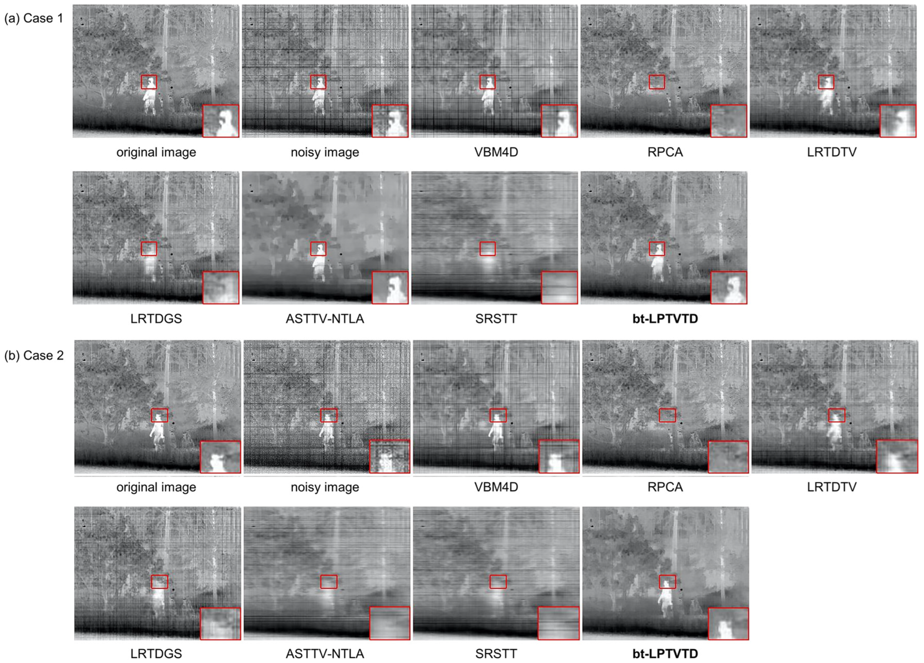
5.1.2. Subjective Evaluation

To subjectively compare the effectiveness of the algorithms, several scenarios from Cases 1 and 2 were selected to compare the denoising results of different algorithms on the same frames of Infrared Dataset 2, as shown in Figure 10. Critical regions were magnified using bilinear interpolation to facilitate visual comparison of denoising effects across various algorithms. For the pointwise and stripewise Gaussian noise in the infrared datasets in Cases 1 and 2, VBM4D, LRTDTV, LRTDGS, ASTTV-NTLA, and SRSTT were unable to effectively suppress stripewise Gaussian noise, and only VBM4D did not blur the moving person. RPCA and bt-LPTVTD were able to effectively suppress both pointwise and stripewise Gaussian noise. However, RPCA completely lost motion information. This is because it flattens the 3D video data into a 2D matrix, destroying the spatial relationships within frames and making motion indistinguishable from noise [76]. In contrast, bt-LPTVTD was able to preserve scene information of both static and moving parts after denoising.

5.1.3. Quantitative Evaluation

The subjective evaluation demonstrates the effectiveness of the bt-LPTVTD method. Subsequently, the objective evaluation metrics of PSNR and SSIM were used to quantitatively analyze the performance of the bt-LPTVTD method in all the simulated experiments, representing the average values of the computed results for all frames in the selected image sequences. Generally, higher PSNR and SSIM values indicate better denoising.
Table 3 shows the evaluation results of the PSNR and SSIM metrics for all the comparison methods under the Case 1 and Case 2 conditions. The best and second-best results among all the comparison methods are highlighted in bold and underlined, respectively, for each metric.
In Cases 1 and 2 of the infrared datasets, the denoising effects of stripewise Gaussian TRN and pointwise TRN were tested under static, moving-target, and moving-camera conditions. While RPCA exhibits superior performance in both static scenes and scenarios with strong mixed noise, primarily attributed to its precise SVD decomposition and robust constraints on sparsity, it sacrifices motion information, which has a minimal impact in these specific contexts. bt-LPTVTD, on the other hand, employs an approximate solution and compromises noise reduction capabilities to retain motion information. This results in a performance inferior to that of RPCA in those two scenarios. However, considering a broader range of scenarios, including those with target motion as observed during surveillance, bt-LPTVTD demonstrates its overall superiority. It effectively completes the denoising task while preserving crucial details in both the static and moving parts of the scene across these cases.
VBM4D exhibits robust denoising stability, maintaining consistent performance in the presence of both stripe and mixed Gaussian noise, even with increased motion areas. However, its PSNR and SSIM metrics are not outstanding. Combined with the results of subjective evaluation, this is likely due to its insufficient suppression of stripe noise. The hyperspectral denoising methods LRTDTV and LRTDGS achieve good performance in background regions. However, their capability drops sharply as the motion area increases. This is consistent with the subjective evaluation, which indicates that the background is well recovered while the human target is blurred. In contrast, the small-target detection methods ASTTV-NTLA and SRSTT are insensitive to the variation in the motion area, but their overall noise suppression ability is limited. Subjective evaluation reveals an overall blurriness in the image, confirming their poor denoising performance.
Figure 11 shows the PSNR and SSIM performance of each method on the infrared datasets. bt-LPTVTD achieves the highest median values in both metrics and has the most compact boxes, indicating its superior and stable performance. In general, using a combination of a twisted tensor model, ASTTV regularization, and a low-rank approximation based on the Laplacian operator, bt-LPTVTD can effectively suppress the TRN while preserving the detailed information of the moving parts. This was validated through simulated experiments using infrared datasets. Moreover, using RPCA on the noise tensor, in contrast to using it directly on the original image tensor, helps to extract finer details within the temporally stationary parts. This significantly improves bt-LPTVTD’s ability to restore static image regions. Benefiting from the aforementioned approach, bt-LPTVTD demonstrates excellent performance in scenarios with partial motion, such as those containing moving targets like pedestrians, and is expected to have a significant beneficial impact in target detection applications for scene monitoring.

5.2. Real Experiments

The equipment used to collect the infrared datasets for real experiments is identical to that used in the simulation experiments. In contrast to the simulation experiment, an overcast and foggy monitoring scenario was deliberately chosen to introduce more pronounced TRN into the collected image sequence, which includes both temporally static and moving components. This allows us to assess the ability of various methods to recover detailed textures and moving targets while suppressing temporal noise.
The denoising results for the infrared datasets are shown in Figure 12, where the yellow vertical lines indicate the vertical slices displayed on the right side of the yellow box. Figure 12a shows that the infrared image exhibits weak pointwise temporal noise. This noise is primarily composed of thermal noise (Gaussian distributed), 1/f noise, and generation-recombination noise, as described in [10] for uncooled IRFPAs. All denoising algorithms were able to improve the noise. However, bt-LPTVTD and VBM4D showed the best visual effects, preserving the clarity of the moving targets while reducing noise. As shown in Figure 12b, the infrared image was contaminated by strong pointwise temporal noise. bt-LPTVTD not only effectively removed noise but also preserved the point target within the red box.

5.3. bt-LPTVTD for Visible Image Denoising

To further demonstrate bt-LPTVTD’s ability to preserve details in static regions and avoid artifacts in dynamic regions, we conducted experiments on visible images. These images, with rich texture and controllable motion (e.g., Figure 13 and Figure 14), allow for clear visual assessment of these denoising aspects, complementing the infrared results. The visible datasets were captured using a Hikvision (Hangzhou, China) industrial camera, MV-CS060-10UM, with a frame rate of 50 Hz, producing grayscale videos. To enhance experimental efficiency, the videos were downsampled to 256 × 320 pixels by extracting odd-numbered rows and columns, following the same approach as with infrared datasets. Similarly to the infrared datasets, Visible Dataset 1 consisted of a static scene with no movement over time. Visible Dataset 2 featured a moving target, where only a person holding a resolution chart moved horizontally at a constant speed. Visible Dataset 3 was captured by a camera moving horizontally at a constant speed, resulting in the entire scene moving uniformly. The simulated noise added to the visible datasets was as follows.
Case 3: Gaussian noise with a mean of zero and variance of 0.005 was added to each frame of the image sequence in the visible datasets for different scenes.
The denoising results are shown in Figure 13 and Table 4. In the noise suppression simulation experiments on the visible datasets, VBM4D performed the best, followed by bt-LPTVTD. The denoising effects of the various contrast algorithms were similar in static scenes. However, when moving objects appeared in a scene, only VBM4D and bt-LPTVTD maintained good denoising effects. Owing to the VBM4D block-matching and 4D filtering strategies, both the PSNR and SSIM achieved leading levels. Figure 15 shows the PSNR and SSIM performance of each method on the visible datasets. VBM4D performed the best, followed by bt-LPTVTD. It is worth noting that the calculations of the PSNR and SSIM were based on individual frames and were then averaged over multiple frames. Even when there was inter-frame variation, VBM4D could achieve a high PSNR and SSIM. Therefore, the best PSNR and SSIM of VBM4D do not necessarily indicate that its TRN denoising effect is the best. This will be verified in subsequent real experiments and can be observed in the slices.
Figure 14 shows the results of the real noise experiments on the visible datasets. The vertical slice at the yellow line is displayed in the yellow box on the right, clearly showing the denoising effect of TRN. It can be seen that the low-light image is severely contaminated by temporal Poisson noise. The noise level improved after denoising using different denoising methods. The LRTDTV, LRTDGS, ASTTV-NTLA, and SRSTT methods either failed to effectively suppress the noise (as shown in Figure 14a) or lost the details of the image (as shown in the red box in Figure 14b). RPCA performs well in denoising the static part but loses the information of the dynamic part. VBM4D performs well under weak noise conditions (as shown in Figure 14b) but can cause detail loss under strong noise conditions (as shown in Figure 15a), and the temporal noise removal is incomplete (as shown in the slice in the yellow box in Figure 14a). bt-LPTVTD has stable denoising effects under both strong and weak noise conditions, achieves denoising while preserving the details of the static and dynamic parts of the image, and has the best visual effect.
The robustness and generalizability of our bt-LPTVTD method were further evaluated by testing its performance on Poisson and mixed noise, noise types frequently encountered in low-light imaging. The results of these additional experiments are available at [https://zenodo.org/doi/10.5281/zenodo.10473803 (accessed on 22 March 2025)].

5.4. Ablation Study

To demonstrate the contribution of each component in bt-LPTVTD, an ablation study was conducted using a 30-frame sequence from Case 3 as an example. The key components, namely the bidirectional twisted tensor, total variation, and RPCA, were individually removed to assess their specific effects and benefits.
Table 5 presents the results of the ablation study on the bidirectional twisted tensor. The results demonstrate that the proposed method effectively enhances restoration performance. Across all three tested scenarios, a significant improvement in PSNR was observed, with an average gain of approximately 0.6 dB. Notably, the experimental results indicate a positive correlation between the proportion of motion regions in the datasets and the performance gain in both PSNR and SSIM, suggesting that a larger motion region proportion leads to more substantial improvements. Furthermore, the significant reduction in the size of each slice in the t-SVD within the proposed method resulted in a considerable improvement in the computational efficiency of the SVD process. The algorithm runtime for all three scenarios decreased from approximately 100 s to approximately 70 s, representing a reduction of approximately 30%, indicating a substantial improvement in algorithm efficiency.
Table 6 presents the results of the ablation study focusing on the impact of TV regularization. The findings unequivocally demonstrate that the integration of TV regularization significantly bolsters restoration performance, yielding a pronounced noise suppression effect. Marked improvements in both PSNR and SSIM metrics were observed across all tested scenarios. Specifically, in the static scenario, the PSNR value exhibited a substantial increase of 3.7753 dB, accompanied by a concomitant rise of 0.1486 in the SSIM. Similarly, in the moving-target scenario, a notable PSNR gain of 2.049 dB and an SSIM enhancement of 0.1174 were recorded. Finally, in the moving-camera scenario, the PSNR value increased by 1.4226 dB, with a corresponding SSIM improvement of 0.1214. These substantial performance gains underscore the inherent limitations of relying solely on the bt-LPTNN method for adaptability across diverse scenarios. The introduction of TV regularization demonstrably enhances the model’s adaptability and robustness, thereby leading to more effective TRN suppression.
Table 7 presents the results of the ablation study on RPCA. The results demonstrate that employing RPCA to extract detailed information from the noise tensor effectively enhances the restoration of static components. The impact of RPCA becomes more significant with an increasing proportion of static temporal elements within the scene. Notably, the PSNR improved by 3.2921 dB, 1.5497 dB, and 0.1118 dB in the static, moving-target, and moving-camera scenarios, respectively, while the SSIM exhibited slight improvements across all scenarios. These gains highlight the effectiveness of RPCA in refining the restoration process, particularly in scenarios with more static content.

5.5. Running Time

All comparative algorithms were run on the same hardware platform, which used an Intel Core i5-8500 @ 3.00 GHz CPU and 16 GB of memory. The average processing time for each frame was obtained by calculating a tensor comprising a sequence of 30 continuous images, as listed in Table 8. Owing to the utilization of the bidirectional twisted tensor, the proposed bt-LPTVTD algorithm is significantly more efficient than the other tensor decomposition algorithms. Additionally, bt-LPTVTD can achieve parallel processing of consecutive tensor blocks by only requiring the collection of 30 continuous frames to form the input tensor without waiting for the computation of the previous tensor to complete. This effectively improved the efficiency of the algorithm in processing consecutive image sequences.

6. Discussion

This study introduces bt-LPTVTD, a novel TRN suppression method for uncooled infrared detectors, based on total variation regularization and low-rank tensor decomposition. This approach has demonstrated significant success in improving image quality, specifically enhancing the Signal-to-Noise Ratio (SNR) and Signal-to-Clutter Ratio (SCR) of processed images. Experimental results confirm that bt-LPTVTD effectively suppresses TRN while preserving essential image details, outperforming several state-of-the-art denoising algorithms across a range of challenging scenarios.
The core of bt-LPTVTD’s effectiveness lies in its combination of ASTTV regularization (for preserving spatial and temporal details), bt-LPTNN (for adaptive weighting and low-rank approximation), and RPCA (for recovering lost spatial information). This approach contrasts with methods that primarily target fixed-pattern noise or those that compromise motion information. While achieving strong denoising performance, bt-LPTVTD currently has a higher computational cost compared to some simpler methods. Therefore, a key focus of future work will be on optimizing computational efficiency through algorithmic improvements and hardware acceleration, enabling its deployment in real-time applications. The demonstrated robustness and detail preservation capabilities of bt-LPTVTD, however, make it a valuable preprocessing step for infrared small target recognition, where increased SNR and SCR are crucial. Beyond this specific application, the method holds promise for broader use in defense, medical imaging, and industrial inspection. Future research will also explore its application to other imaging modalities and the development of more comprehensive video quality metrics.

7. Conclusions

This paper proposes a bidirectional twisted tensor truncated nuclear norm (bt-LPTNN) based on the Laplace operator to effectively suppress TRN in low-signal-to-noise-ratio infrared and visible images. The bt-LPTNN can adaptively assign different weights to all singular values, and the bidirectional twisted tensor can better capture temporal information while preserving horizontal and vertical spatial domain information. In addition, the weighted spatiotemporal total variation regularization nonconvex tensor approximation method can fully utilize prior structural information and better preserve detailed textures. Furthermore, the use of RPCA on the noise tensor can effectively extract spatial domain information, resulting in a better performance of the algorithm in static scenes. These improvements constitute the proposed bt-LPTVTD method, whose main contributions include the following:
(1)
A bidirectional twisted tensor truncated nuclear norm based on the Laplacian operator combined with a weighted spatiotemporal total variation regularization nonconvex tensor approximation method is proposed. The bidirectional twisted tensor can better capture temporal information while preserving horizontal and vertical spatial information. The improved tensor recovery estimation method demonstrates more significant TRN suppression and more effectively preserves moving-target details.
(2)
To recover spatial information that may be lost during the tensor estimation process, RPCA is further utilized to extract spatial information from the noise tensor. As a result, the proposed method achieves improved detail recovery for the static components of the scene.
(3)
An augmented Lagrange multiplier algorithm is designed to solve the proposed bt-LPTVTD model.
Numerous experimental results demonstrate that, compared to existing methods that combine TV and tensor decomposition, the bt-LPTVTD method exhibits a superior TRN suppression effect while considering scene adaptability and robustness, not only providing better denoising performance but also showing strong adaptability to various noise types and scene conditions.
Future research will be directed toward developing a suitable method for FPN suppression during the tensor decomposition process, with the objective of achieving simultaneous suppression of both types of noise. In addition, denoising algorithms with high operational efficiencies will be developed for engineering applications, and further investigations will be conducted to develop simplification methods for the bt-LPTVTD model to improve its operational speed and expand its application scope to diverse scenarios. Future work also includes the development of more suitable video quality metrics that account for temporal information.

Supplementary Materials

The following supporting information (video version of the experimental results) can be downloaded at: https://zenodo.org/doi/10.5281/zenodo.10473803 (accessed on 22 March 2025), Figure 10: case1.avi, case2.avi; Figure 12: real1.avi, real2.avi; Figure 13: case3.avi; Figure 14: real3.avi, real4.avi.

Author Contributions

Z.L. and W.J. proposed the original idea. Z.L. performed the experiments and wrote the manuscript. L.L. reviewed and edited the manuscript. All authors have read and agreed to the published version of the manuscript.

Funding

This work was supported in part by the National Natural Science Foundation of China under Grant 61871034 and in part by the Equipment Advance Research Field Fund Project under Grant 61404140513.

Data Availability Statement

The original contributions presented in the study are included in the article/Supplementary Materials, further inquiries can be directed to the corresponding author.

Conflicts of Interest

The authors declare no conflicts of interest.

References

  1. Planinsic, G. Infrared Thermal Imaging: Fundamentals, Research and Applications. Eur. J. Phys. 2011, 32, 1431. [Google Scholar] [CrossRef]
  2. Rogalski, A. Infrared detectors: An overview. Infrared Phys. Technol. 2002, 43, 187–210. [Google Scholar] [CrossRef]
  3. Kruer, M.R.; Scribner, D.A.; Killiany, J.M. Infrared Focal Plane Array Technology Development for Navy Applications. Opt. Eng. 1987, 26, 263182. [Google Scholar] [CrossRef]
  4. Qu, Z.; Jiang, P.; Zhang, W. Development and Application of Infrared Thermography Non-Destructive Testing Techniques. Sensors 2020, 20, 3851. [Google Scholar] [CrossRef] [PubMed]
  5. Kaltenbacher, E.; Hardie, R.C. High Resolution Infrared Image Reconstruction Using Multiple, Low Resolution, Aliased Frames. In Proceedings of the IEEE 1996 National Aerospace and Electronics Conference NAECON 1996, Dayton, OH, USA, 20–22 May 1996; Volume 2, pp. 702–709. [Google Scholar]
  6. Ring, E.F.J.; Ammer, K. Infrared thermal imaging in medicine. Physiol. Meas. 2012, 33, R33–R46. [Google Scholar] [CrossRef]
  7. Jing, Z.; Li, S.; Zhang, Q. YOLOv8-STE: Enhancing Object Detection Performance Under Adverse Weather Conditions with Deep Learning. Electronics 2024, 13, 5049. [Google Scholar] [CrossRef]
  8. Scribner, D.A.; Kruer, M.R.; Killiany, J.M. Infrared focal plane array technology. Proc. IEEE 1991, 79, 66–85. [Google Scholar] [CrossRef]
  9. Rogalski, A. Infrared detectors: Status and trends. Prog. Quantum Electron. 2003, 27, 59–210. [Google Scholar] [CrossRef]
  10. Feng, T.; Jin, W.-Q.; SI, J.-J.; Zhang, H.-J. Optimal theoretical study of the pixel structure and spatio-temporal random noise of uncooled IRFPA. J. Infrared Millim. Waves 2020, 39, 143–148. [Google Scholar]
  11. Yuan, P.; Tan, Z.; Zhang, X.; Wang, M.; Jin, W.; Li, L.; Su, B. Fixed-pattern noise model for filters in uncooled infrared focal plane array imaging optical paths. Infrared Phys. Technol. 2023, 133, 104790. [Google Scholar] [CrossRef]
  12. Steffanson, M.; Gorovoy, K.; Holz, M.; Ivanov, T.; Kampmann, R.; Kleindienst, R.; Sinzinger, S.; Rangelow, I.W. Low-Cost Uncooled Infrared Detector Using Thermomechanical Micro-Mirror Array with Optical Readout. In Proceedings of the Proceedings IRS2 2013, Nurnberg, Germany, 14–16 May 2013; AMA Service GmbH: Wunstorf, Germany, 2013; pp. 85–88. [Google Scholar]
  13. Zhang, Y.; Chen, X.; Rao, P.; Jia, L. Dim Moving Multi-Target Enhancement with Strong Robustness for False Enhancement. Remote Sens. 2023, 15, 4892. [Google Scholar] [CrossRef]
  14. Wang, Y.; Pan, N.; Jiang, P. Anisotropic Filtering Based on the WY Distribution and Multiscale Energy Concentration Accumulation Method for Dim and Small Target Enhancement. Remote Sens. 2024, 16, 3069. [Google Scholar] [CrossRef]
  15. Aliha, A.; Liu, Y.; Zhou, G.; Hu, Y. High-Speed Spatial–Temporal Saliency Model: A Novel Detection Method for Infrared Small Moving Targets Based on a Vectorized Guided Filter. Remote Sens. 2024, 16, 1685. [Google Scholar] [CrossRef]
  16. Lu, X.; Li, F. Study of Robust Visual Tracking Based on Traditional Denoising Methods and CNN. In Proceedings of the 2021 International Conference on Security, Pattern Analysis, and Cybernetics (SPAC), Chengdu, China, 18–20 June 2021; pp. 392–396. [Google Scholar]
  17. Li, J.; Wang, W.; Tivnan, M.; Stayman, J.W.; Gang, G.J. Performance Assessment Framework for Neural Network Denoising. In Proceedings of the Medical Imaging 2022: Physics of Medical Imaging; Zhao, W., Yu, L., Eds.; SPIE: San Diego, CA, USA, 2022; p. 64. [Google Scholar]
  18. Huang, Y.; Sun, G.; Xing, M. A SAR Image Denoising Method for Target Shadow Tracking Task. In Proceedings of the 6th International Conference on Digital Signal Processing, Chengdu China, 25–27 February 2022; ACM: New York, NY, USA, 2022; pp. 164–169. [Google Scholar]
  19. Tang, J.; Zhang, F.; Ma, F.; Gao, F.; Yin, Q.; Zhou, Y. How SAR Image Denoise Affects the Performance of DCNN-Based Target Recognition Method. In Proceedings of the 2021 IEEE International Geoscience and Remote Sensing Symposium IGARSS, Brussels, Belgium, 11–16 July 2021; pp. 3609–3612. [Google Scholar]
  20. Liu, X.; Bourennane, S.; Fossati, C. Reduction of Signal-Dependent Noise from Hyperspectral Images for Target Detection. IEEE Trans. Geosci. Remote Sens. 2014, 52, 5396–5411. [Google Scholar] [CrossRef]
  21. Endo, K.; Yamamoto, K.; Ohtsuki, T. A Denoising Method Using Deep Image Prior to Human-Target Detection Using MIMO FMCW Radar. Sensors 2022, 22, 9401. [Google Scholar] [CrossRef]
  22. Wei, Y.; Sun, B.; Zhou, Y.; Wang, H. Non-Line-of-Sight Moving Target Detection Method Based on Noise Suppression. Remote Sens. 2022, 14, 1614. [Google Scholar] [CrossRef]
  23. Sun, Q.; Liu, X.; Bourennane, S.; Liu, B. Multiscale denoising autoencoder for improvement of target detection. Int. J. Remote Sens. 2021, 42, 3002–3016. [Google Scholar] [CrossRef]
  24. Hou, F.; Zhang, Y.; Zhou, Y.; Zhang, M.; Lv, B.; Wu, J. Review on Infrared Imaging Technology. Sustainability 2022, 14, 11161. [Google Scholar] [CrossRef]
  25. Li, Y.; Jin, W.; Zhu, J.; Zhang, X.; Li, S. An Adaptive Deghosting Method in Neural Network-Based Infrared Detectors Nonuniformity Correction. Sensors 2018, 18, 211. [Google Scholar] [CrossRef]
  26. Li, Y.; Jin, W.; Liu, Z. Interior Radiation Noise Reduction Method Based on Multiframe Processing in Infrared Focal Plane Arrays Imaging System. IEEE Photonics J. 2018, 10, 6803512. [Google Scholar] [CrossRef]
  27. Li, Y.; Jin, W.; Li, S.; Zhang, X.; Zhu, J. A method of sky ripple residual nonuniformity reduction for a cooled infrared imager and hardware implementation. Sensors 2017, 17, 1070. [Google Scholar] [CrossRef] [PubMed]
  28. Lv, B.; Tong, S.; Liu, Q.; Sun, H. Statistical Scene-Based Non-Uniformity Correction Method with Interframe Registration. Sensors 2019, 19, 5395. [Google Scholar] [CrossRef]
  29. Sheng, Y.; Dun, X.; Jin, W.; Zhou, F.; Wang, X.; Mi, F.; Xiao, S. The On-Orbit Non-Uniformity Correction Method with Modulated Internal Calibration Sources for Infrared Remote Sensing Systems. Remote Sens. 2018, 10, 830. [Google Scholar] [CrossRef]
  30. Rota, C.; Buzzelli, M.; Bianco, S.; Schettini, R. Video restoration based on deep learning: A comprehensive survey. Artif. Intell. Rev. 2023, 56, 5317–5364. [Google Scholar] [CrossRef]
  31. Liang, J.; Cao, J.; Fan, Y.; Zhang, K.; Ranjan, R.; Li, Y.; Timofte, R.; Van Gool, L. Vrt: A video restoration transformer. arXiv 2022, arXiv:2201.12288. [Google Scholar] [CrossRef] [PubMed]
  32. Tassano, M.; Delon, J.; Veit, T. FastDVDnet: Towards Real-Time Deep Video Denoising Without Flow Estimation. In Proceedings of the IEEE/CVF Conference on Computer Vision and Pattern Recognition, Seattle, WA, USA, 13–19 June 2020; pp. 1351–1360. [Google Scholar]
  33. Zhang, K.; Zuo, W.; Chen, Y.; Meng, D.; Zhang, L. Beyond a Gaussian Denoiser: Residual Learning of Deep CNN for Image Denoising. IEEE Trans. Image Process. 2017, 26, 3142–3155. [Google Scholar] [CrossRef]
  34. Tassano, M.; Delon, J.; Veit, T. DVDNET: A Fast Network for Deep Video Denoising. In Proceedings of the 2019 IEEE International Conference on Image Processing (ICIP), Taipei, China, 22–25 September 2019; pp. 1805–1809. [Google Scholar]
  35. Sheth, D.Y.; Mohan, S.; Vincent, J.L.; Manzorro, R.; Crozier, P.A.; Khapra, M.M.; Simoncelli, E.P.; Fernandez-Granda, C. Unsupervised Deep Video Denoising. In Proceedings of the 2021 IEEE/CVF International Conference on Computer Vision (ICCV), Montreal, BC, Canada, 11–17 October 2021; pp. 1759–1768. [Google Scholar]
  36. Chan, K.C.K.; Zhou, S.; Xu, X.; Loy, C.C. BasicVSR\mathplus\mathplus: Improving Video Super-Resolution with Enhanced Propagation and Alignment. In Proceedings of the 2022 IEEE/CVF Conference on Computer Vision and Pattern Recognition (CVPR), New Orleans, LA, USA, 18–24 June 2022. [Google Scholar]
  37. Song, M.; Zhang, Y.; Aydın, T.O. TempFormer: Temporally Consistent Transformer for Video Denoising. In Proceedings of the European Conference on Computer Vision (ECCV), Tel Aviv, Israel, 23–27 October 2022; Springer: Cham, Switzerland, 2022; pp. 481–496. [Google Scholar]
  38. Menghani, G. Efficient Deep Learning: A Survey on Making Deep Learning Models Smaller, Faster, and Better. ACM Comput. Surv. 2023, 55, 259. [Google Scholar] [CrossRef]
  39. Maggioni, M.; Boracchi, G.; Foi, A.; Egiazarian, K. Video Denoising, Deblocking, and Enhancement Through Separable 4-D Nonlocal Spatiotemporal Transforms. IEEE Trans. Image Process. 2012, 21, 3952–3966. [Google Scholar] [CrossRef]
  40. Maggioni, M.; Katkovnik, V.; Egiazarian, K.; Foi, A. Nonlocal Transform-Domain Filter for Volumetric Data Denoising and Reconstruction. IEEE Trans. Image Process. 2013, 22, 119–133. [Google Scholar] [CrossRef]
  41. Sutour, C.; Deledalle, C.-A.; Aujol, J.-F. Adaptive Regularization of the NL-Means: Application to Image and Video Denoising. IEEE Trans. Image Process. 2014, 23, 3506–3521. [Google Scholar] [CrossRef]
  42. Arias, P.; Morel, J.-M. Video Denoising via Empirical Bayesian Estimation of Space-Time Patches. J. Math. Imaging Vis. 2018, 60, 70–93. [Google Scholar] [CrossRef]
  43. Li, M.; Liu, J.; Sun, X.; Xiong, Z. Image/Video Restoration via Multiplanar Autoregressive Model and Low-Rank Optimization. ACM Trans. Multimed. Comput. Commun. Appl. 2019, 15, 102. [Google Scholar] [CrossRef]
  44. Ji, H.; Liu, C.; Shen, Z.; Xu, Y. Robust video denoising using low rank matrix completion. In Proceedings of the 2010 IEEE Computer Society Conference on Computer Vision and Pattern Recognition, San Francisco, CA, USA, 13–18 June 2010; pp. 1791–1798. [Google Scholar]
  45. Zhang, X.; Yuan, X.; Carin, L. Nonlocal Low-Rank Tensor Factor Analysis for Image Restoration. In Proceedings of the 2018 IEEE/CVF Conference on Computer Vision and Pattern Recognition, Salt Lake City, UT, USA, 18–22 June 2018; pp. 8232–8241. [Google Scholar]
  46. Shen, B.; Kamath, R.R.; Choo, H.; Kong, Z. Robust Tensor Decomposition Based Background/Foreground Separation in Noisy Videos and Its Applications in Additive Manufacturing. IEEE Trans. Autom. Sci. Eng. 2021, 20, 583–596. [Google Scholar] [CrossRef]
  47. Gui, L.; Cui, G.; Zhao, Q.; Wang, D.; Cichocki, A.; Cao, J. Video Denoising Using Low Rank Tensor Decomposition. In Proceedings of the Ninth International Conference on Machine Vision (ICMV 2016), Nice, France, 18–20 November 2016; SPIE: San Diego, CA, USA, 2017; Volume 10341, pp. 162–166. [Google Scholar]
  48. Fan, H.; Li, C.; Guo, Y.; Kuang, G.; Ma, J. Spatial–Spectral Total Variation Regularized Low-Rank Tensor Decomposition for Hyperspectral Image Denoising. IEEE Trans. Geosci. Remote Sens. 2018, 56, 6196–6213. [Google Scholar] [CrossRef]
  49. Wang, Y.; Peng, J.; Zhao, Q.; Leung, Y.; Zhao, X.-L.; Meng, D. Hyperspectral Image Restoration Via Total Variation Regularized Low-Rank Tensor Decomposition. IEEE J. Sel. Top. Appl. Earth Obs. Remote Sens. 2018, 11, 1227–1243. [Google Scholar] [CrossRef]
  50. Li, J.; Zhang, P.; Zhang, L.; Zhang, Z. Sparse Regularization-Based Spatial–Temporal Twist Tensor Model for Infrared Small Target Detection. IEEE Trans. Geosci. Remote Sens. 2023, 61, 5000417. [Google Scholar] [CrossRef]
  51. Liu, T.; Yang, J.; Li, B.; Xiao, C.; Sun, Y.; Wang, Y.; An, W. Nonconvex Tensor Low-Rank Approximation for Infrared Small Target Detection. IEEE Trans. Geosci. Remote Sens. 2022, 60, 5614718. [Google Scholar] [CrossRef]
  52. Lee, C.; Wang, M. Tensor Denoising and Completion Based on Ordinal Observations. In InInternational Conference on Machine Learning; PMLR: New York, NY, USA, 2020; pp. 5778–5788. [Google Scholar]
  53. Gong, X.; Chen, W.; Chen, J.; Ai, B. Tensor Denoising Using Low-Rank Tensor Train Decomposition. IEEE Signal Process. Lett. 2020, 27, 1685–1689. [Google Scholar] [CrossRef]
  54. Bi, Y.; Lu, Y.; Long, Z.; Zhu, C.; Liu, Y. Tensors for Data Processing; Elsevier: Amsterdam, The Netherlands, 2022. [Google Scholar]
  55. Claus, M.; Gemert, J.V. ViDeNN: Deep Blind Video Denoising. In Proceedings of the 2019 IEEE/CVF Conference on Computer Vision and Pattern Recognition Workshops (CVPRW), Long Beach, CA, USA, 16–20 June 2019; pp. 1843–1852. [Google Scholar]
  56. Monakhova, K.; Richter, S.R.; Waller, L.; Koltun, V. Dancing Under the Stars: Video Denoising in Starlight. In Proceedings of the 2022 IEEE/CVF Conference on Computer Vision and Pattern Recognition (CVPR), New Orleans, LA, USA, 18–24 June 2022; pp. 16220–16230. [Google Scholar]
  57. Wu, C.; Gao, T. Image Denoise Methods Based on Deep Learning. J. Phys. Conf. Ser. 2021, 1883, 012112. [Google Scholar] [CrossRef]
  58. Reeja, S.R.; Kavya, N.P. Real Time Video Denoising. In Proceedings of the 2012 IEEE International Conference on Engineering Education: Innovative Practices and Future Trends (AICERA), Kottayam, India, 19–21 July 2012; pp. 1–5. [Google Scholar]
  59. Han, J.; Kopp, T.; Xu, Y. An estimation-theoretic approach to video denoiseing. In Proceedings of the 2015 IEEE International Conference on Image Processing (ICIP), Quebec City, QC, Canada, 27–30 September 2015; pp. 4273–4277. [Google Scholar]
  60. Ponomaryov, V.I.; Montenegro-Monroy, H.; Gallegos-Funes, F.; Pogrebnyak, O.; Sadovnychiy, S. Fuzzy color video filtering technique for sequences corrupted by additive Gaussian noise. Neurocomputing 2015, 155, 225–246. [Google Scholar] [CrossRef]
  61. Samantaray, A.; Bhattacharya, S. Fast Trilateral Filtering for Video Denoising. In Proceedings of the 2020 IEEE 5th International Conference on Computing Communication and Automation (ICCCA), Greater Noida, India, 30–31 October 2020; pp. 554–558. [Google Scholar]
  62. Hu, W.; Tao, D.; Zhang, W.; Xie, Y.; Yang, Y. The Twist Tensor Nuclear Norm for Video Completion. IEEE Trans. Neural Netw. Learn. Syst. 2017, 28, 2961–2973. [Google Scholar] [CrossRef] [PubMed]
  63. Qiu, Y.; Zhou, G.; Zhao, Q.; Xie, S. Noisy Tensor Completion via Low-Rank Tensor Ring. IEEE Trans. Neural Netw. Learn. Syst. 2022, 35, 1127–1141. [Google Scholar] [CrossRef]
  64. Chen, Y.; He, W.; Yokoya, N.; Huang, T.-Z. Hyperspectral Image Restoration Using Weighted Group Sparsity-Regularized Low-Rank Tensor Decomposition. IEEE Trans. Cybern. 2020, 50, 3556–3570. [Google Scholar] [CrossRef]
  65. Hu, T.; Li, W.; Liu, N.; Tao, R.; Zhang, F.; Scheunders, P. Hyperspectral Image Restoration Using Adaptive Anisotropy Total Variation and Nuclear Norms. IEEE Trans. Geosci. Remote Sens. 2021, 59, 1516–1533. [Google Scholar] [CrossRef]
  66. Zheng, Y.-B.; Huang, T.-Z.; Zhao, X.-L.; Jiang, T.-X.; Ma, T.-H.; Ji, T.-Y. Mixed Noise Removal in Hyperspectral Image via Low-Fibered-Rank Regularization. IEEE Trans. Geosci. Remote Sens. 2020, 58, 734–749. [Google Scholar] [CrossRef]
  67. Sun, Y.; Yang, J.; Long, Y.; An, W. Infrared Small Target Detection via Spatial-Temporal Total Variation Regularization and Weighted Tensor Nuclear Norm. IEEE Access 2019, 7, 56667–56682. [Google Scholar] [CrossRef]
  68. Zhang, P.; Zhang, L.; Wang, X.; Shen, F.; Pu, T.; Fei, C. Edge and Corner Awareness-Based Spatial–Temporal Tensor Model for Infrared Small-Target Detection. IEEE Trans. Geosci. Remote Sens. 2021, 59, 10708–10724. [Google Scholar] [CrossRef]
  69. Li, X.; Ye, Y.; Xu, X. Low-Rank Tensor Completion with Total Variation for Visual Data Inpainting. Proc. AAAI Conf. Artif. Intell. 2017, 31, 2210–2216. [Google Scholar] [CrossRef]
  70. He, W.; Yokoya, N.; Yuan, L.; Zhao, Q. Remote Sensing Image Reconstruction Using Tensor Ring Completion and Total Variation. IEEE Trans. Geosci. Remote Sens. 2019, 57, 8998–9009. [Google Scholar] [CrossRef]
  71. Wang, Y.; Lin, L.; Zhao, Q.; Yue, T.; Meng, D.; Leung, Y. Compressive Sensing of Hyperspectral Images via Joint Tensor Tucker Decomposition and Weighted Total Variation Regularization. IEEE Geosci. Remote Sens. Lett. 2017, 14, 2457–2461. [Google Scholar] [CrossRef]
  72. Xu, T.; Huang, T.-Z.; Deng, L.-J.; Zhao, X.-L.; Huang, J. Hyperspectral Image Superresolution Using Unidirectional Total Variation with Tucker Decomposition. IEEE J. Sel. Top. Appl. Earth Obs. Remote Sens. 2020, 13, 4381–4398. [Google Scholar] [CrossRef]
  73. Sun, L.; Zhan, T.; Wu, Z.; Jeon, B. A Novel 3D Anisotropic Total Variation Regularized Low Rank Method for Hyperspectral Image Mixed Denoising. ISPRS Int. J. Geo-Inf. 2018, 7, 412. [Google Scholar] [CrossRef]
  74. Xu, W.-H.; Zhao, X.-L.; Ji, T.-Y.; Miao, J.-Q.; Ma, T.-H.; Wang, S.; Huang, T.-Z. Laplace function based nonconvex surrogate for low-rank tensor completion. Signal Process. Image Commun. 2019, 73, 62–69. [Google Scholar] [CrossRef]
  75. Goyette, N.; Jodoin, P.-M.; Porikli, F.; Konrad, J.; Ishwar, P. Changedetection.net: A New Change Detection Benchmark Dataset. In Proceedings of the 2012 IEEE Computer Society Conference on Computer Vision and Pattern Recognition Workshops, Rhode Island, RI, USA, 16–21 June 2012; pp. 1–8. [Google Scholar]
  76. Wen, F.; Ying, R.; Liu, P.; Qiu, R.C. Robust PCA Using Generalized Nonconvex Regularization. IEEE Trans. Circuits Syst. Video Technol. 2020, 30, 1497–1510. [Google Scholar] [CrossRef]
  77. Boyd, S. Distributed Optimization and Statistical Learning via the Alternating Direction Method of Multipliers. FNT Mach. Learn. 2010, 3, 1–122. [Google Scholar] [CrossRef]
Figure 1. Temporal noise suppression performance of LRTDTV [49] and ASTTV-NTLA [51]: (a) original image, (b) image with Gaussian noise, (c) LRTDTV denoised image, (d) ASTTV-NTLA denoised image 1, and (e) ASTTV-NTLA denoised image 2.
Remotesensing 17 01343 g001
Figure 2. Illustration of the Mode-3 t-SVD.
Remotesensing 17 01343 g002
Figure 3. Comparison of the l0 norm, l1 norm, Laplace norm, and Log norm for a singular value.
Remotesensing 17 01343 g003
Figure 4. Overall framework of the proposed TRN denoise bt-LPTVTD model.
Remotesensing 17 01343 g004
Figure 5. Spatial and temporal correlation of infrared image sequences.
Remotesensing 17 01343 g005
Figure 6. Horizontal twist, vertical twist, and squeezing of the tensor. The blue arrow indicates the direction of Mode-3.
Remotesensing 17 01343 g006
Figure 7. Denoising result of (11), obtained using a denoising model. (a) Noisy image, (b) denoised image, and (c) noise image.
Remotesensing 17 01343 g007
Figure 8. Noise tensor before and after applying the RPCA.
Remotesensing 17 01343 g008
Figure 9. Change in objective function values versus the iteration number of bt-LPTVTD.
Remotesensing 17 01343 g009
Figure 10. Simulation experiments on the Infrared Dataset 2.
Remotesensing 17 01343 g010
Figure 11. Boxplots of PSNR and SSIM for different methods on infrared datasets. (a) PSNR results, (b) SSIM results.
Remotesensing 17 01343 g011
Figure 12. Real experiments on the infrared datasets. (a) Scene 1, (b) Scene 2. Yellow lines indicate vertical slices, and the red box highlights area for detailed comparison.
Remotesensing 17 01343 g012
Figure 13. Simulation experiments on Visible Dataset 2. The red and green boxes highlight areas for detailed comparison.
Remotesensing 17 01343 g013
Figure 14. Real experiments on the visible datasets. (a) Scene 1, (b) Scene 2. Yellow lines indicate vertical slices, and the red and green boxes highlight areas for detailed comparison.
Remotesensing 17 01343 g014
Figure 15. Boxplots of PSNR and SSIM for different methods on visible datasets. (a) PSNR results, (b) SSIM results.
Remotesensing 17 01343 g015
Table 1. Notations.
Table 1. Notations.
NotationsExplanations
X / X / x / x Tensor/Matrix/Vector/Scalar
X i , j , k The (i, j, k)-th element
X : , : , k or X ( k ) / X : , j , : / X i , : , : Temporal/Vertical/Horizontal slice
X i The i-th iteration value of X
X ( i ) R n i × k i n k Mode-i decomposition of tensor X
X , Y Inner product of tensors X and Y
X F Frobenius norm of tensor X
X * Nuclear norm of tensor X , the sum of all singular values
Y = X × n U The Mode-n product of X and U , represented in matrix form as Y ( n ) = U X ( n )
X The twisted tensor of X
Table 2. Parameter settings for comparative algorithms.
Comparative AlgorithmsParameter SettingsOutput Data
2D algorithm expansionVBM4Dprofile = ‘np’, do_wiener = 0, sharpen = 1, deflicker = 0.5, verbose = 1, est_noise = 1Denoised Tensor Y
RPCAλ = 0.003Denoised Tensor L ,
Noise Tensor S
Hyperspectral image denoising algorithmsLRTDTVτ = 1, λ = 100,000, β = 100Denoised Tensor X ,
Noise Tensor S + N
LRTDGSλ1 = 0.8, λ2 = 10Denoised Tensor X ,
Noise Tensor S + N
Small object detection algorithmsASTTV-NTLAλtv = 0.01, λs = 0.1, λ3 = 0.5Denoised Tensor B + T ,
Noise Tensor N
SRSTTλ1 = 10,000, λ2 = 0.1, λ3 = 0.5Denoised Tensor B + T ,
Noise Tensor N
The proposed algorithmbt-LPTVTDλ = 0.0005, β = 0.01, λN = 0.003Denoised Tensor X + T ,
Noise Tensor M
Table 3. Quantitative comparisons of all the comparative methods for infrared datasets under different noise conditions (Bold = Best PSNR/SSIM; Underline = Second-best PSNR/SSIM).
DatasetsCasesIndexNoisyVBM4DRPCALRTDTVLRTDGSASTTV-NTLASRSTTbt-LPTVTD
Infrared Dataset 1 (Static)Case 1PSNR21.258721.983228.157324.676026.821823.830222.606326.7460
SSIM0.60200.59070.90830.83060.81690.66540.61230.8754
Case 2PSNR19.905922.505923.372924.653523.704622.477822.633225.1003
SSIM0.47130.60590.89610.82260.78150.60490.61150.8707
Infrared Dataset 2 (Moving Target)Case 1PSNR21.106921.918325.734424.671326.700324.550522.630827.0484
SSIM0.48590.48510.87280.77480.76400.68760.53400.8358
Case 2PSNR19.927122.679522.295524.682523.748222.571622.604925.3411
SSIM0.36070.52570.86020.77230.70870.53930.53730.8858
Infrared Dataset 3 (Moving Camera)Case 1PSNR21.220521.820620.810323.091324.154223.763421.507224.8054
SSIM0.50510.51570.53140.65050.61000.70840.49230.7374
Case 2PSNR19.884522.607219.769923.057122.615121.504621.470923.0607
SSIM0.37510.56460.50950.63880.57970.49120.48850.6556
Table 4. Quantitative comparisons of all the comparative methods for visible datasets (Bold = Best PSNR/SSIM; Underline = Second-best PSNR/SSIM).
DatasetsIndexNoisyVBM4DRPCALRTDTVLRTDGSASTTV-NTLASRSTTbt-LPTVTD
Visible Dataset 1 (Static)PSNR23.047133.210630.903432.097631.863028.622925.691232.3759
SSIM0.51070.90610.90760.90650.89980.81510.78380.9147
Visible Dataset 2 (Moving Target)PSNR23.078831.830123.604927.067926.737227.044222.856130.3463
SSIM0.53840.89930.77280.80570.79690.79010.68880.8894
Visible Dataset 3 (Moving Camera)PSNR23.061829.926319.602824.998224.655926.191620.863328.4749
SSIM0.51490.87670.51440.72690.70320.77200.54070.8506
Table 5. Ablation experiments on bidirectional twisted tensors. Bold = Best result.
DatasetsIndexNoisy ImageWith Bidirectional Twisted TensorWithout Bidirectional Twisted Tensor
Visible Dataset 1 (Static)PSNR23.04332.694832.3837
SSIM0.51320.92410.9216
Running time (s)/69.681599.5749
Visible Dataset 2 (Moving Target)PSNR23.072829.569228.8052
SSIM0.54630.88570.8705
Running time (s)/70.982394.9965
Visible Dataset 3 (Moving Camera)PSNR23.070228.92628.0386
SSIM0.51090.86840.8456
Running time (s)/69.9584101.4699
Table 6. Ablation experiments on total variations. Bold = Best result.
DatasetsIndexNoisy ImageWith Bidirectional Twisted TensorWithout Bidirectional Twisted Tensor
Visible Dataset 1 (Static)PSNR23.04332.694828.9195
SSIM0.51320.92410.7755
Visible Dataset 2 (Moving Target)PSNR23.072829.569227.5202
SSIM0.54630.88570.7683
Visible Dataset 3 (Moving Camera)PSNR23.070228.92627.5034
SSIM0.51090.86840.7470
Table 7. Ablation experiments on RPCA. Bold = Best result.
DatasetsIndexNoisy ImageWith Bidirectional Twisted TensorWithout Bidirectional Twisted Tensor
Visible Dataset 1 (Static)PSNR23.04332.694829.4027
SSIM0.51320.92410.8487
Visible Dataset 2 (Moving Target)PSNR23.072829.569228.0195
SSIM0.54630.88570.8419
Visible Dataset 3 (Moving Camera)PSNR23.070228.92628.8142
SSIM0.51090.86840.8654
Table 8. Running time (seconds).
MethodsVBM4DRPCALRTDTVLRTDGSASTTV-NTLASRSTTbt-LPTVTD
Running time6.78561.428811.13447.891011.833829.01002.0809
Disclaimer/Publisher’s Note: The statements, opinions and data contained in all publications are solely those of the individual author(s) and contributor(s) and not of MDPI and/or the editor(s). MDPI and/or the editor(s) disclaim responsibility for any injury to people or property resulting from any ideas, methods, instructions or products referred to in the content.

