Author Contributions
Conceptualization, T.J.; methodology, T.J. and F.Z.; software, T.J.; validation, T.J., F.Z. and Y.X. (Yi Xie); formal analysis, C.Z.; investigation, L.C. and Y.X. (Yihao Xu); resources, Y.X. (Yihao Xu); data curation, H.T.; writing—original draft preparation, T.J.; writing—review and editing, F.Z. and Y.X. (Yi Xie); visualization, C.Z.; supervision, H.T.; project administration, L.C.; funding acquisition, L.C. All authors have read and agreed to the published version of the manuscript.
Figure 1.
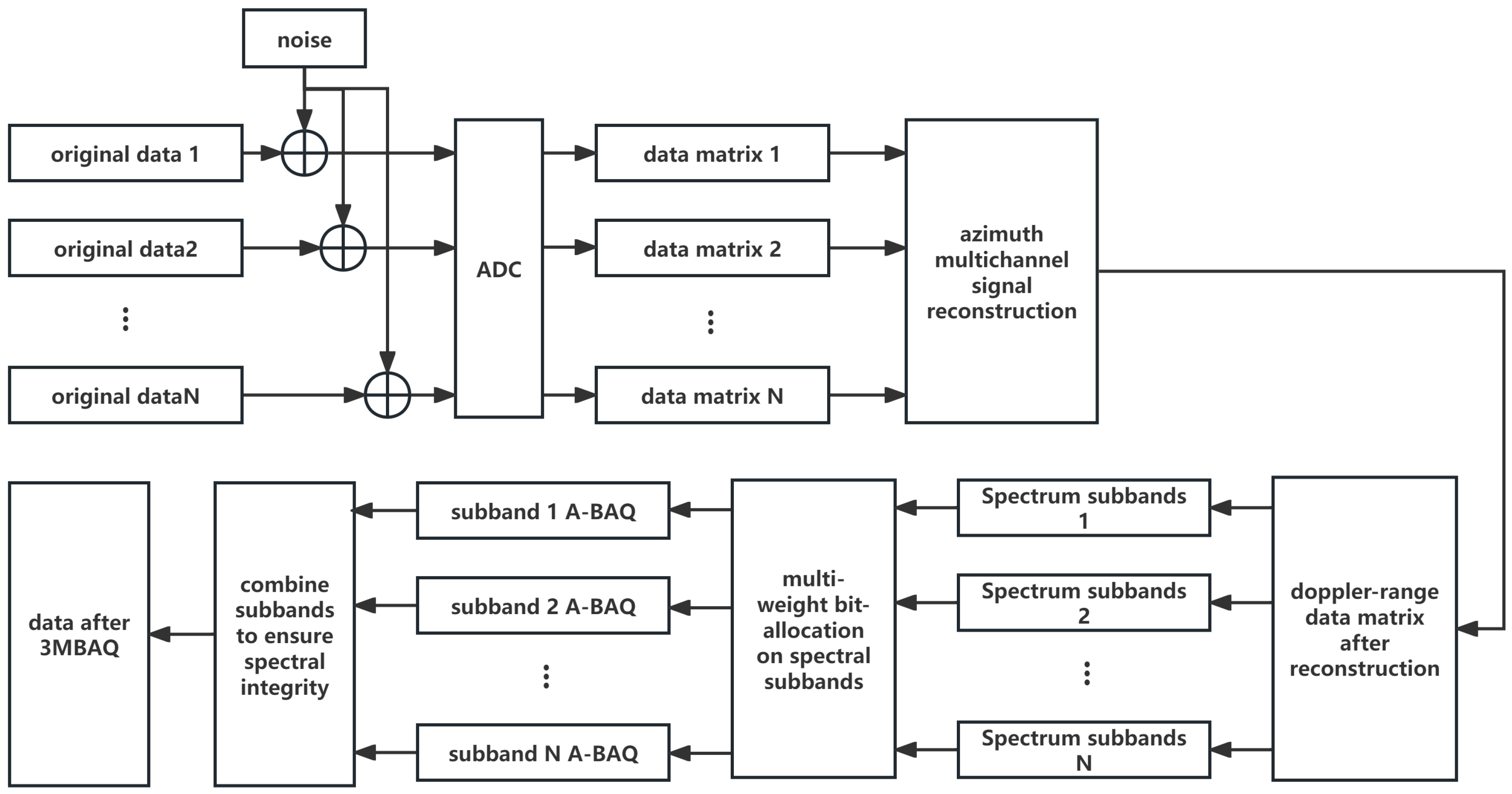
Flowchart of the 3MBAQ algorithm [
34].
Figure 1.
Flowchart of the 3MBAQ algorithm [
34].
Figure 2.
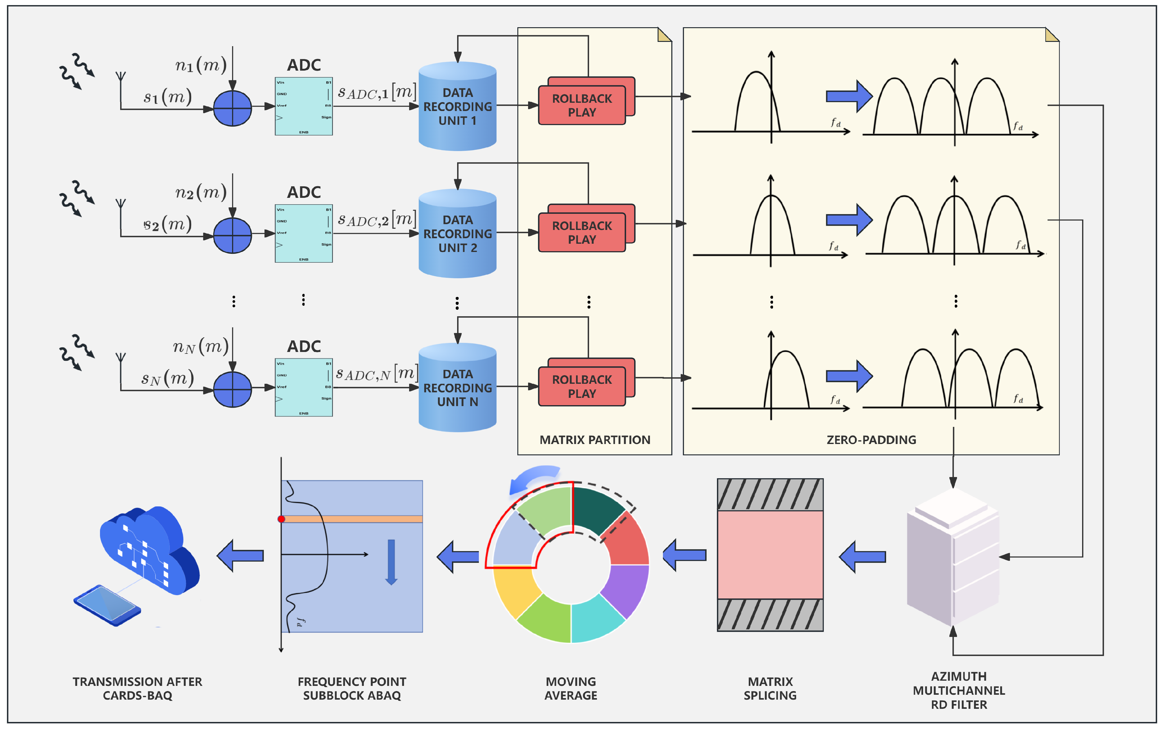
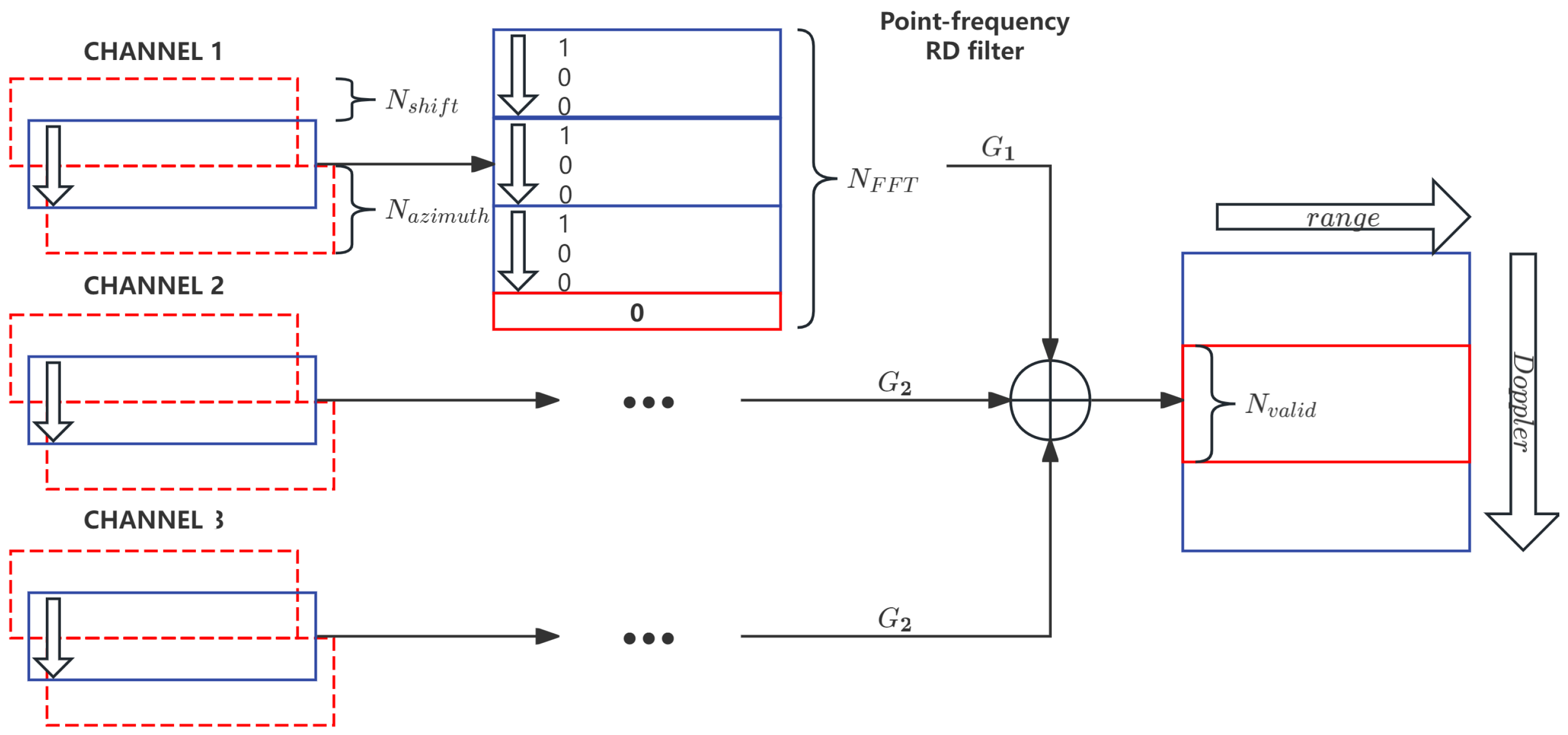
Flowchart of the CARDS-BAQ algorithm. By rolling back and replaying the multi-channel data, azimuth multi-channel RD domain filtering is performed through matrix partitioning. The data are then further spliced and processed with moving averaging, followed by single-frequency-point sub-block ABAQ processing. Here, N represents the number of azimuth channels, which is generally a non-power-of-two number.
Figure 2.
Flowchart of the CARDS-BAQ algorithm. By rolling back and replaying the multi-channel data, azimuth multi-channel RD domain filtering is performed through matrix partitioning. The data are then further spliced and processed with moving averaging, followed by single-frequency-point sub-block ABAQ processing. Here, N represents the number of azimuth channels, which is generally a non-power-of-two number.
Figure 3.
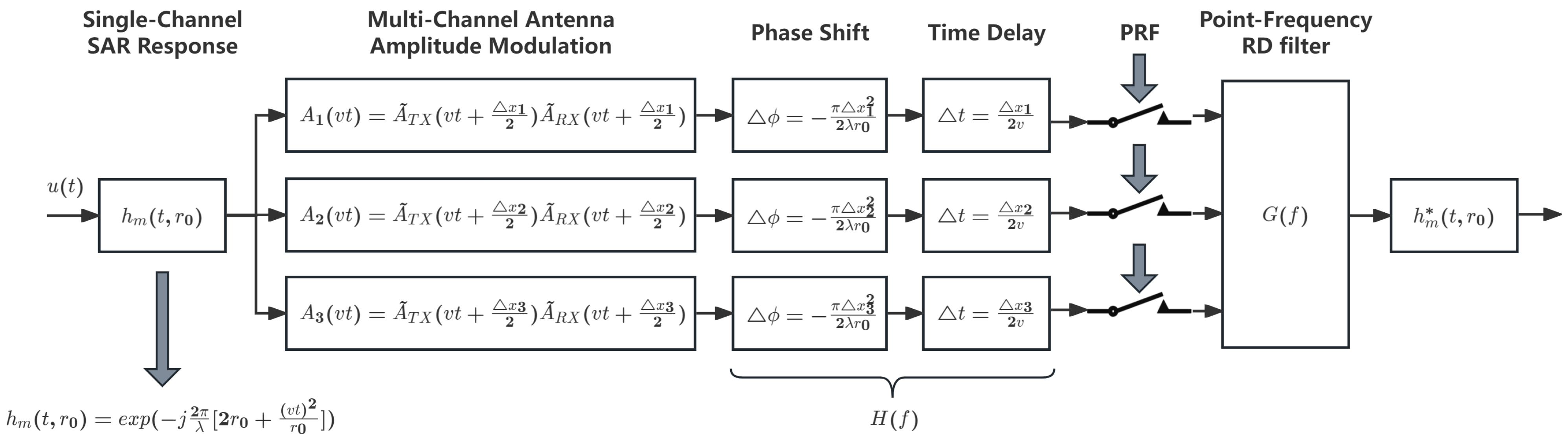
Signal reconstruction process using the point-frequency filter, illustrated with a 3-channel example.
Figure 3.
Signal reconstruction process using the point-frequency filter, illustrated with a 3-channel example.
Figure 4.
Logical diagram of 3-channel output data splicing processing.
Figure 4.
Logical diagram of 3-channel output data splicing processing.
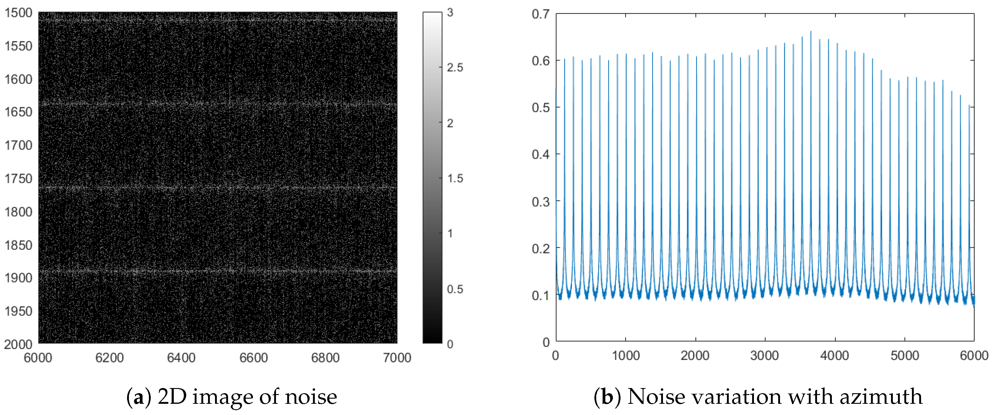
Figure 5.
Diagram of noise in the SAR image without stitching correction, exhibiting periodic variations along the azimuth direction. (a) 2D image of noise; (b) periodically varying stitching noise in the azimuth direction.
Figure 5.
Diagram of noise in the SAR image without stitching correction, exhibiting periodic variations along the azimuth direction. (a) 2D image of noise; (b) periodically varying stitching noise in the azimuth direction.
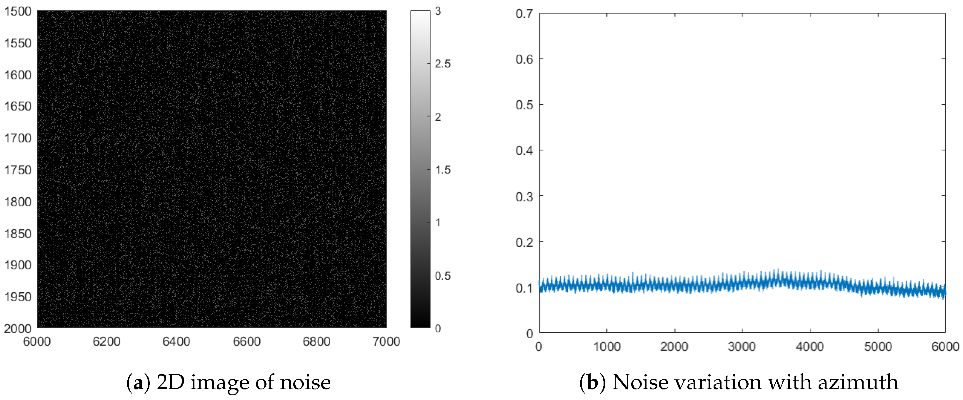
Figure 6.
Diagram of noise in the SAR image after sub-block stitching compensation, where periodic noise patterns are significantly suppressed. (a) 2D image of noise; (b) periodically varying stitching noise in the azimuth direction.
Figure 6.
Diagram of noise in the SAR image after sub-block stitching compensation, where periodic noise patterns are significantly suppressed. (a) 2D image of noise; (b) periodically varying stitching noise in the azimuth direction.
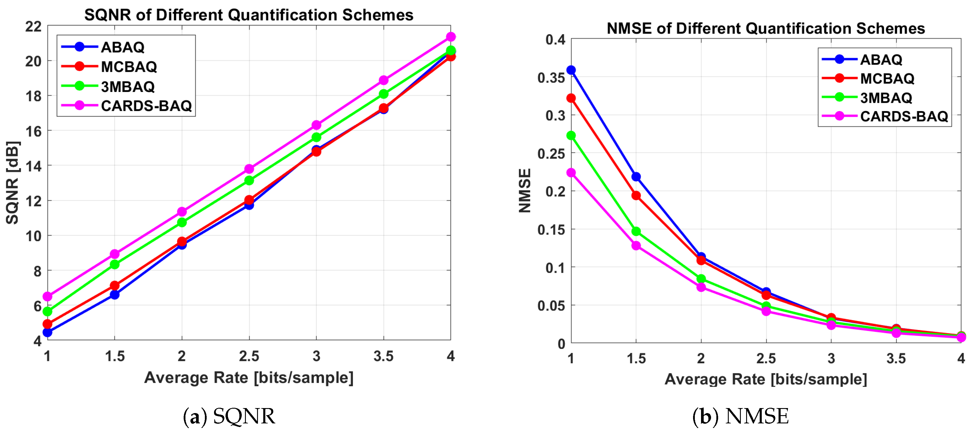
Figure 7.
SQNR and NMSE curves versus bit rates for different data compression schemes. The curves are color-coded as follows: 3MBAQ in green, MCBAQ in red, ABAQ in blue, and CARDS-BAQ in purple. Note that the curves for BAQ and ABAQ overlap at integer points, and, since BAQ does not support non-integer compression, its curve is not shown.
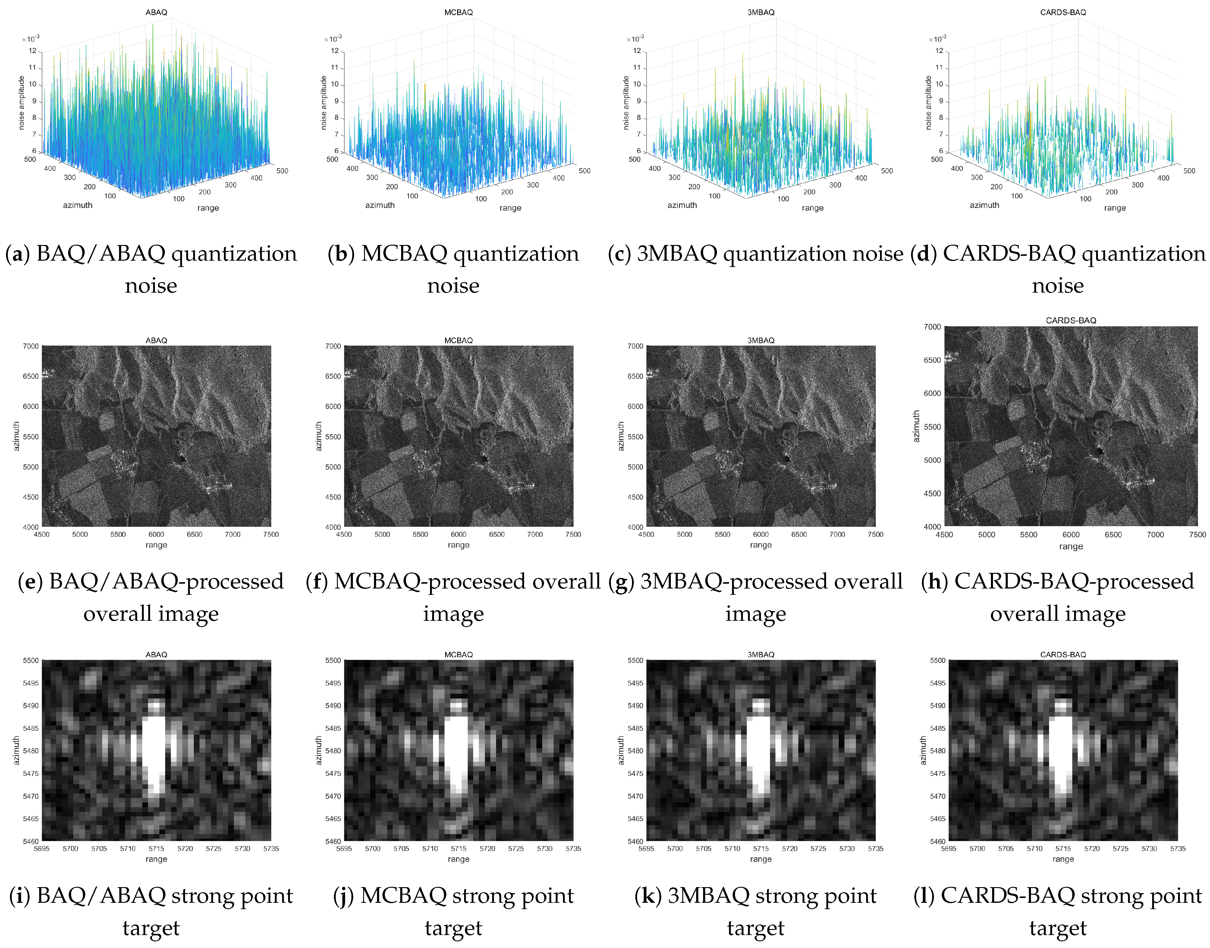
Figure 8.
Comparison of CARDS-BAQ with BAQ/ABAQ, MCBAQ, and 3MBAQ in the image domain. (a–d) The 3D quantization noise maps for BAQ/ABAQ, MCBAQ, 3MBAQ, and CARDS-BAQ, respectively. (e–h) The overall image compression results in the image domain for the four algorithms. (i–l) The strong-point-target performance for the four algorithms.
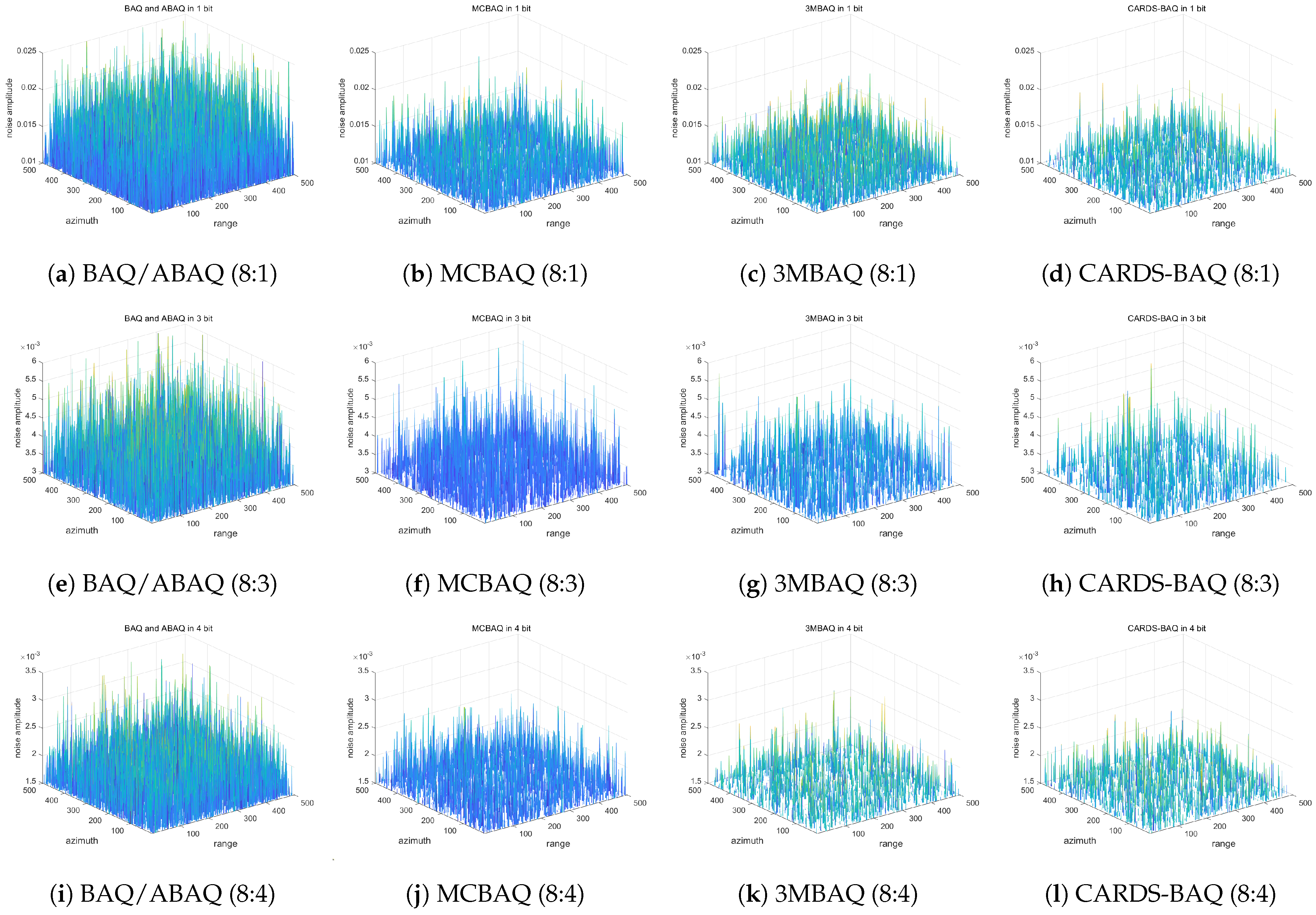
Figure 9.
3D plots of image-domain quantization noise under different compression methods at compression ratios of 8:1, 8:3, and 8:4. (a–d) The quantization noise of BAQ/ABAQ, MCBAQ, 3MBAQ, and CARDS-BAQ at an 8:1 compression ratio, respectively. (e–h) The results at an 8:3 compression ratio. (i–l) The results at an 8:4 compression ratio.
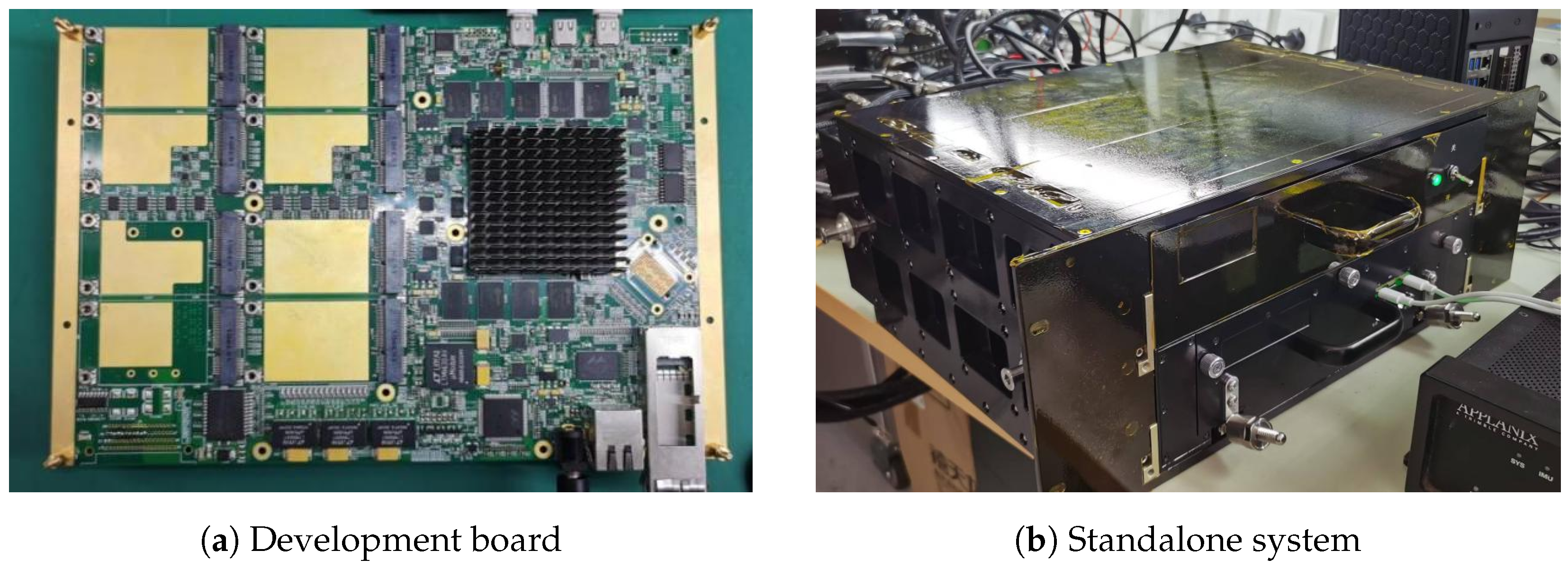
Figure 10.
Xilinx V7 development board and data compression standalone system.
Figure 10.
Xilinx V7 development board and data compression standalone system.
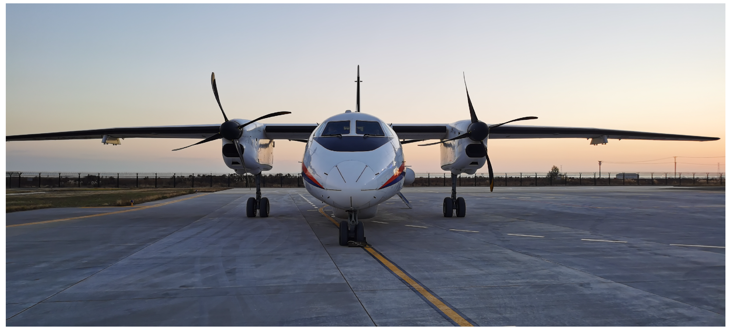
Figure 11.
Payload platform of the wide-swath SAR project.
Figure 11.
Payload platform of the wide-swath SAR project.
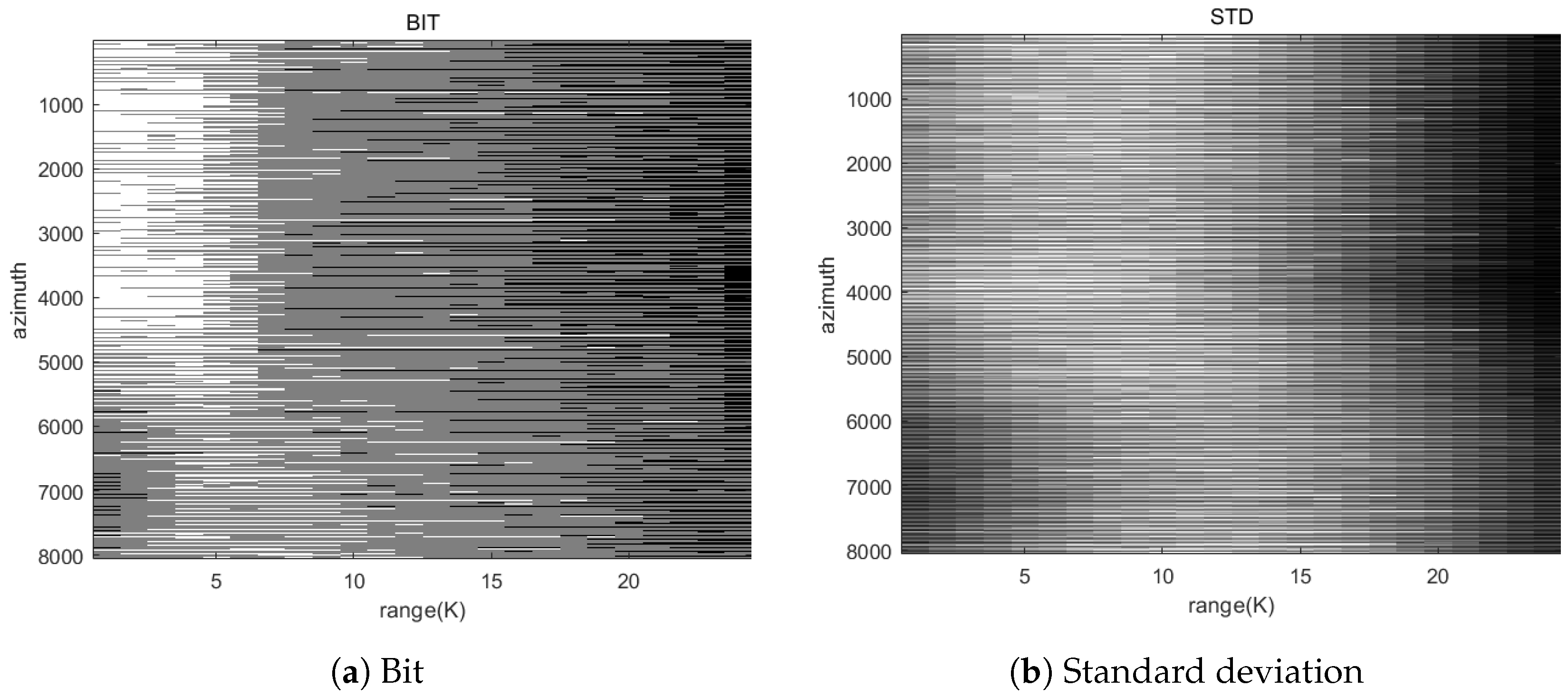
Figure 12.
Auxiliary file information obtained after data compression by FPGA. (a) Adaptive bit allocation for data block; (b) standard deviation for each data block.
Figure 12.
Auxiliary file information obtained after data compression by FPGA. (a) Adaptive bit allocation for data block; (b) standard deviation for each data block.
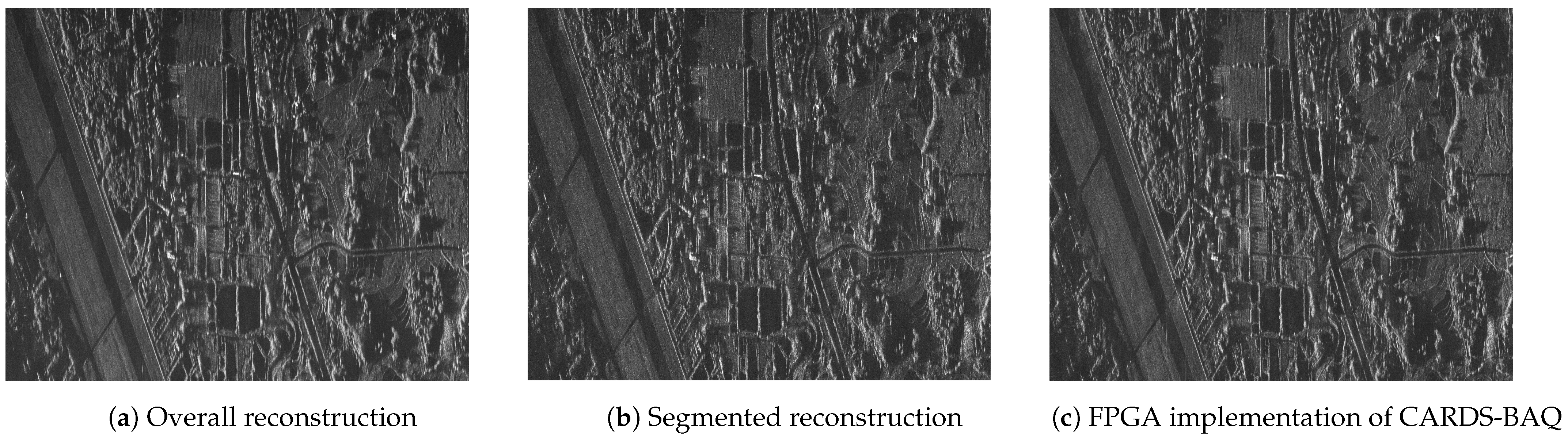
Figure 13.
Comparison of images obtained after FPGA data compression and decompression. (a) Overall reconstruction of the original data; (b) segmented reconstruction of the original data; (c) imaging obtained after decompression by FPGA implementation.
Figure 13.
Comparison of images obtained after FPGA data compression and decompression. (a) Overall reconstruction of the original data; (b) segmented reconstruction of the original data; (c) imaging obtained after decompression by FPGA implementation.
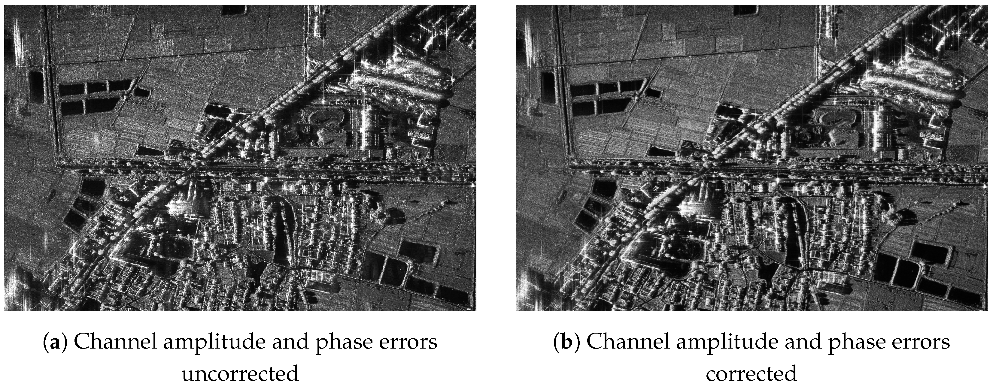
Figure 14.
Performance of CARDS-BAQ in flight data in Yingkou, Liaoning Province, China, in 2024. (a) Imaging after CARDS-BAQ compression; (b) imaging after multi-channel error correction processing.
Figure 14.
Performance of CARDS-BAQ in flight data in Yingkou, Liaoning Province, China, in 2024. (a) Imaging after CARDS-BAQ compression; (b) imaging after multi-channel error correction processing.
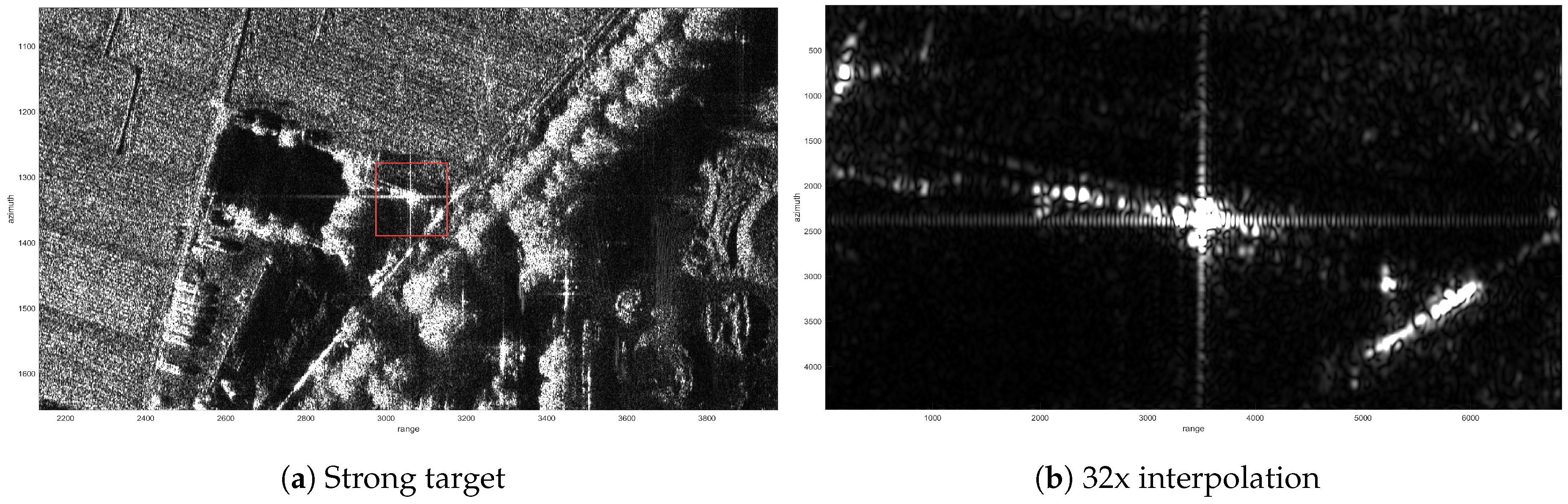
Figure 15.
Strong target selection range. (a) Strong target locations in red box; (b) 32× interpolation.
Figure 15.
Strong target selection range. (a) Strong target locations in red box; (b) 32× interpolation.
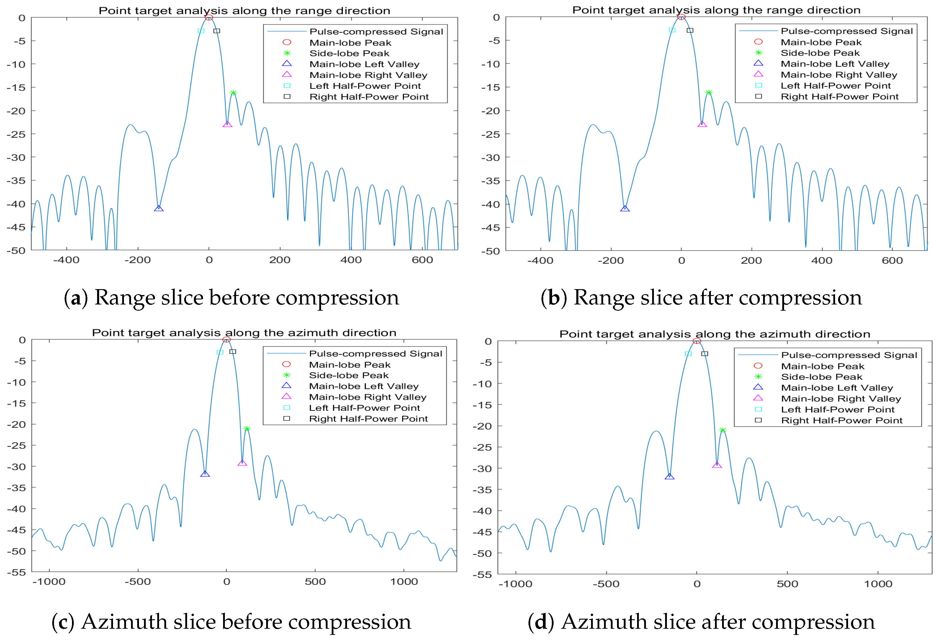
Figure 16.
Two-dimensional profile of strong target.
Figure 16.
Two-dimensional profile of strong target.
Table 1.
Partial parameters of GF-3 data.
Table 1.
Partial parameters of GF-3 data.
| Parameter | Value |
|---|
| Number of azimuth channels, N | 2 |
| Frequency band | C |
| Azimuth antenna length, | 7.5 m |
| Pulse repetition frequency, | 2179 Hz |
| Total processed bandwidth, | 2466 Hz |
| Minimum slant range, | 902,273 m |
| Effective radar velocity, | 7133 m/s |
| Range sample frequency, | 133 MHz |
| Range bandwidth, | 120 MHz |
Table 2.
Performance of 5 data compression algorithms at different compression ratios on GF-3 data.
Table 2.
Performance of 5 data compression algorithms at different compression ratios on GF-3 data.
| Index | Ratio | BAQ | ABAQ | MCBAQ | 3MBAQ | CARDS-BAQ |
|---|
| SQNR | 8:1 | 4.4518 | 4.4518 | 4.9234 | 5.6423 | 6.4982 |
| 8:2 | 9.4566 | 9.4566 | 9.6458 | 10.7385 | 11.3476 |
| 8:3 | 14.8848 | 14.8848 | 14.7778 | 15.6083 | 16.3055 |
| 8:4 | 20.5168 | 20.5168 | 20.2248 | 20.5788 | 21.3546 |
| NMSE | 8:1 | 0.3588 | 0.3588 | 0.3219 | 0.2728 | 0.0224 |
| 8:2 | 0.1133 | 0.1133 | 0.1085 | 0.0844 | 0.0733 |
| 8:3 | 0.0325 | 0.0325 | 0.0333 | 0.0275 | 0.0234 |
| 8:4 | 0.0089 | 0.0089 | 0.0095 | 0.0088 | 0.0073 |
Table 3.
Hardware and software environments of CARDS-BAQ.
Table 3.
Hardware and software environments of CARDS-BAQ.
| Parameter | Value |
|---|
| Project device part | xc7vx690tffg1927-2 |
| DDR3 model | UniIC-HXI15H4G160AF-13K |
| Amount of SDRAM | 9 |
| Internal organization | 8 banks × 32 M bits × 16 |
| Vivado edition | 2018.1 |
| Windows edition | Win10 |
| System clock | 100 MHz |
Table 4.
Resource utilization of FPGA implementation on V7 development board.
Table 4.
Resource utilization of FPGA implementation on V7 development board.
| Resource | Utilization | Available | Utilization % |
|---|
| LUT | 223,646 | 433,200 | 51.63 |
| LUTRAM | 34,466 | 174,200 | 19.79 |
| FF | 318,634 | 866,400 | 36.78 |
| BRAM | 1221.5 | 1470 | 83.10 |
| DSP | 1682 | 3600 | 46.72 |
Table 5.
Partial parameters of the wide-swath SAR project data.
Table 5.
Partial parameters of the wide-swath SAR project data.
| Parameter | Value |
|---|
| Number of azimuth channels, N | 3 |
| Frequency band | X |
| Azimuth antenna length, | 1.5 m |
| Pulse repetition frequency, | 1000 Hz |
| Minimum slant range, | 15,000 m |
| Effective radar velocity, | 124 m/s |
| Range sample frequency, | 800 MHz |
| Range bandwidth, | 600 MHz |
Table 6.
FPGA performance based on ABAQ compression in spaceborne multi-channel SAR Doppler domain.
Table 6.
FPGA performance based on ABAQ compression in spaceborne multi-channel SAR Doppler domain.
| | Compared with Overall Reconstruction | Compared with Segmentation Reconstruction |
|---|
| | Complex | I | Q | Complex | I | Q |
|---|
| Ratio 1 | ≥8:2 |
| Ratio 2 | 8:1.9826 |
| SQNR (dB) | 10.7653 | 10.7699 | 10.7607 | 10.9047 | 10.9093 | 10.9001 |
| NMSE | 0.0838 | 0.0838 | 0.0839 | 0.0812 | 0.0811 | 0.0813 |
Table 7.
Comparison of imaging quality in range and azimuth directions.
Table 7.
Comparison of imaging quality in range and azimuth directions.
| | Azimuth | Range |
|---|
| | ORIGIN | CARDS-BAQ | LOSS | ORIGIN | CARDS-BAQ | LOSS |
|---|
| PSLR (dB) | −21.02 | −20.71 | 0.31 | −16.13 | −15.97 | 0.16 |
| ISLR (dB) | −18.67 | −17.73 | 0.84 | −14.51 | −14.02 | 0.49 |
| IRW (m) | 0.558 | 0.554 | 0.004 | 0.263 | 0.263 | 0 |


 ,
, 
