A Machine Learning Algorithm Using Texture Features for Nighttime Cloud Detection from FY-3D MERSI L1 Imagery

Abstract

Accurate cloud detection is critical for quantitative applications of satellite-based advanced imager observations, yet nighttime cloud detection presents challenges due to the lack of visible and near-infrared spectral information. Nighttime cloud detection using infrared (IR)-only information needs to be improved. Based on a collocated dataset from Fengyun-3D Medium Resolution Spectral Imager (FY-3D MERSI) Level 1 data and CALIPSO CALIOP lidar Level 2 product, this study proposes a novel framework leveraging Light Gradient-Boosting Machine (LGBM), integrated with grey level co-occurrence matrix (GLCM) features extracted from IR bands, to enhance nighttime cloud detection capabilities. The LGBM model with GLCM features demonstrates significant improvements, achieving an overall accuracy (OA) exceeding 85% and an F1-Score (F1) of nearly 0.9 when validated with an independent CALIOP lidar Level 2 product. Compared to the threshold-based algorithm that has been used operationally, the proposed algorithm exhibits superior and more stable performance across varying solar zenith angles, surface types, and cloud altitudes. Notably, the method produced over 82% OA over the cryosphere surface. Furthermore, compared to LGBM models without GLCM inputs, the enhanced model effectively mitigates the thermal stripe effect of MERSI L1 data, yielding more accurate cloud masks. Further evaluation with collocated MODIS-Aqua cloud mask product indicates that the proposed algorithm delivers more precise cloud detection (OA: 90.30%, F1: 0.9397) compared to that of the MODIS product (OA: 84.66%, F1: 0.9006). This IR-alone algorithm advancement offers a reliable tool for nighttime cloud detection, significantly enhancing the quantitative applications of satellite imager observations.

1. Introduction

Clouds play a crucial role in the evolution of weather and climate [1,2], the global hydrological cycle [3,4], and the global radiative budget [5]. With an average annual coverage of a range of 60~70% [6,7,8], cloud detection is an essential and fundamental task in optical remote sensing processing because clouds can obstruct the view of the Earth’s surface, therefore affecting downstream applications. Over the past decades, the extensive utilization of optical remote sensing measurements with moderate resolutions from polar-orbit satellites in cloud retrieval has been attributed to their high spatiotemporal consistency. Additionally, this type of data can also offer a wealth of spectral information, covering a wide range from visible to near-infrared and thermal infrared wavelengths, which is beneficial to obtaining promising cloud masks. Traditional cloud detection processes adopted threshold-based algorithms, based on the underlying physics of spectral and brightness temperature structures of clouds, to produce cloud cover products [9,10]. For instance, the procedure of the MODIS cloud mask product applied several spectral tests to determine the confidence of the observations being unobstructed by clouds [9,10,11,12]. Previous studies assessing MODIS cloud mask data revealed underestimation of clouds over the cryosphere [13], retrieval issues with the omission of optically thin clouds [12], high detection uncertainty during nighttime [14], and the misclassification of thick aerosols as clouds [15]. The thresholds defined and tuned manually cannot cope with the complexity of nonlinear retrieval tasks [16], such as detecting thin clouds and clouds near similar backgrounds [17]. Furthermore, it is essential to consider that the thresholds must be modified based on the specific characteristics of the satellite view geometry [15].

Machine learning (ML) techniques have gained significant attention in the remote sensing community for image classification tasks. ML algorithms can learn patterns and relationships from a large amount of labeled training data and then apply that knowledge to classify new and unseen images. The advantage of using ML techniques is that they can handle high-dimensional data, capture complex relationships between features, and adapt to different types of remote sensing imagery [18]. They can also improve the accuracy and efficiency of image classification compared to traditional manual or rule-based methods. Specifically, studies adopted ML algorithms to conduct cloud detection from optical satellite remote sensing imagery. For example, a support vector machine trained by labeled data using Discriminate Analysis was employed to retrieve cloud cover from MODIS data [19]. The method produced a high agreement of cloud mask with MODIS 35 [19].

Using the corresponding Level 2 cloud product as ground truth allows for developing deep learning (DL) algorithms of semantic segmentation. Wang et al. [20], for example, used MYD06 and MYD35 to train the proposed TIR-CNN algorithm, based on the U-Net architecture, to classify clouds. The algorithm provided around 94% classification accuracy during both daytime and nighttime [18]. Likewise, the U-Net-based models were applied on FY-4A [21] and MSG [22] for cloud detection using their corresponding Level 2 cloud products. However, the Level 2 product was produced by traditional threshold-based algorithms, as mentioned before, thereby introducing bias and uncertainty into the training dataset. Additionally, the development of segmentation-style DL networks proposed by recent research [23,24,25] should rely on two-dimensional manual labels where each pixel is designated as either the clear sky or cloud. Nighttime manual labeling is significantly challenging due to the absence of solar illumination, and even with the use of false color composites from IR bands, discriminating clouds from clear sky remains difficult under conditions such as, high water vapor and the presence of ice/snow. Moreover, the implementation of DL models often requires significant computation resources, resulting in challenges when attempting to apply these models on a global scale.

In recent years, the tree-based ensemble algorithms trained by using active lidar and radar observations as ground truth (e.g., CALIPSO CALIOP Lidar, CloudSat Cloud Profiling Radar) were implemented to conduct cloud detection. For example, random forest produced more than 97% cloud detection accuracy from MODIS over the tropical forests in Amazonia [26]. Furthermore, cloud detection procedures based on random forest demonstrated accuracy levels exceeding 90% in the case of VIIRS [27], Himawari-8 [16], and FY-2G [28]. An advanced tree-based ensemble algorithm, XGBoost, was applied to generate cloud cover mask data from Himawari-8 with approximately 90% detection accuracy [29]. Among ML models, the Light Gradient-Boosting Machine (LGBM) proposed by Microsoft in 2017 [30] has indeed gained significant attention in recent years as a research hotspot of remote sensing in a variety of study topics, such as inland water and ocean [31,32,33], geomorphology [34,35], land use and urban [36,37], and forest [38]. Meanwhile, many studies have indicated the outperformance of LGBM in various Earth observation retrieval tasks using satellite remote sensing data compared to other ML models [39,40,41,42]. The reasons behind its popularity are its notable advantages, including fast training speed, low resource consumption, strong generalization ability, and resistance to overfitting. However, fewer studies have addressed the practicability of the LGBM algorithm for cloud detection from optical remote sensing data.

Nevertheless, previous studies mainly focused on the evaluation of daytime cloud detection performance by incorporating visible and near-infrared spectral channels of optical remote sensing data. The comprehensive examination and analysis of cloud retrieval from optical remote sensing data with moderate spatial resolutions using ML algorithms have received limited attention thus far. Furthermore, nighttime cloud detection indeed poses a significant challenge in the field of optical remote sensing classification due to the absence of sufficient solar illumination sources, resulting in the limited availability of optical spectral information, such as visible and near-infrared channels.

Besides cloud detection, numerous studies employed ML algorithms to retrieve cloud properties from moderate optical remote sensing data, such as cloud top phase [43,44], cloud top height [29,45,46], cloud base height [43,47], cloud types [43,48,49], and cloud optical thickness [20,45]. Notwithstanding, cloud detection is the most fundamental and crucial initial step in retrieving various cloud properties. Meanwhile, there is a significant lack of experimental studies focused on the assessment and analysis of ML algorithms for nighttime cloud detection capability in the field of remote sensing. Therefore, this research attempts to examine the feasibility of improved nighttime cloud detection by using an ML algorithm from moderate optical remote sensing polar-orbit imagery.

Gray level co-occurrence matrix (GLCM) is a second-order texture analysis algorithm to delineate image textures by extracting the spatial relationship of image pixel intensities [50,51]. Hence, GLCM measures have been widely applied to conduct image classification tasks of remote sensing in various fields [52,53,54,55,56,57,58,59]. Compared to classification based solely on remote sensing observations, the utilization of GLCM is able to improve the classification performance since the textures provide valuable insights and information regarding the direction, adjacent intervals, and variation range of the pixel gray values [60]. Clouds present unique textural properties depending on their type. For instance, Cirrus clouds exhibit a smooth, filamentous texture with high contrast due to their sparse, wispy structure, while Cumulus clouds display a lumpy texture with lower contrast and higher homogeneity due to their vertical development and shading [61]. Implementing GLCM features showed promising cloud detection performance from remote sensing imagery with a high spatial resolution [62]. Furthermore, during the daytime, the integration of ML algorithms with GLCM measures enables faithful cloud detection in moderate optical remote sensing images [61]. Therefore, in order to enhance the spatial information, this study incorporates the GLCM algorithm into the development of LGBM so as to improve nighttime cloud detection.

In the past decades, a number of Chinese meteorological satellites, the FengYun (FY) series, have been providing large volumes of remote sensing data that play important roles in global weather services and Earth research. The second-generation Medium Resolution Spectral Imager (MERSI-II) is a major optical sensor onboard FY-3D, which is a polar-orbit satellite, providing global daily Earth observations used in many studies [63,64,65]. Starting from January 2019, the MERSI-II Level 1 products have been made available to users worldwide through the website of the National Satellite Meteorological Center of China (http://satellite.nsmc.org.cn (accessed on 5 January 2024)). Thus, the development of promising and accurate cloud detection algorithms is crucial for effectively utilizing the MERSI-II Level 1 products. Moreover, the proposed algorithm should be transferred to FY-3H, which will succeed and build upon the legacy of the FY-3D.

The study presents three key contributions:

• Development of an operational nighttime cloud detection algorithm framework for FY-3D MERSI based on LGBM, which is more robust than current operational methods.
• Integration of spatial texture to enhance model robustness under various conditions and to mitigate the effects of thermal stripes inherent in MERSI Level 1 imagery.
• Introduction of a comprehensive multi-aspect assessment framework that addresses the complexities and challenges associated with nighttime cloud detection across different algorithms.

2. Materials and Methods

2.1. Data

2.1.1. FY-3D MERSI-II Products

The MERSI-II instrument on the FY-3D satellite has been providing the L1 imagery since 2018. It consists of 25 spectral bands, including visible, near-infrared, middle infrared, and thermal infrared. These bands allow for the measurement of surface and atmospheric variables such as land surface temperature, soil moisture, aerosols, and clouds. One notable ability of MERSI-II is to capture global thermal infrared split-window data with a spatial resolution of 250 m. In order to develop the nighttime cloud detection algorithm, the six thermal infrared channels were employed. The channel specifications are shown in

Table 1. Key Specifications of the MERSI-II L1 thermal channels.

Band	Central Wavelength (µm)	Spectral Bandwidth (nm)	IFOV *	Dynamic Range
BT20	3.80	180	1000	200–350 K
BT21	4.05	155	1000	200–380 K
BT22	7.20	500	1000	180–280 K
BT23	8.55	300	1000	180–300 K
BT24	10.80	1000	250	180–330 K
BT25	12.00	1000	250	180–330 K

* IFOV denotes the instantaneous field of view in meters, representing the spatial resolution of the sensor.

. For the algorithm development, the two 250 m channels were aggerated to 1 km observations.

The MERSI-II cloud mask (CLM) product utilizes L1 observations from visible and infrared spectral channels (bands 3, 4, 6, 7, 19, 20, 21, 24, 25) to determine whether a pixel is cloudy or clear sky [66]. This is achieved through a multi-threshold classification process that takes into account different underlying surfaces [66]. The product provides information on four categories: cloudy, possibly cloudy, possibly clear sky, and clear sky stored in HDF5 format with 1 km. The cloud mask field in the files within the scientific dataset contains six layers and is stored in binary mode. The detection results are shown in the first layer. In this study, CLM pixels of cloudy and possibly cloudy were treated as clouds, while possibly clear and clear were considered to clear sky.

2.1.2. CALIPSO

The CALIOP instrument, onboard the CALIPSO since 2006, is an active lidar that uses two wavelengths (532 nm and 1064 nm) to probe the vertical profiles of aerosols and clouds [67]. With a horizontal resolution of 333 m and vertical resolutions of 30–60 m, this product has been extensively utilized as ground truth or validation data in cloud-related research [29,44,46,68]. In this analysis, the latest version (Version 4.51) of the Level 2 cloud layer product was selected to extract ground truth labels. One of the variables, the number of layers found, was used to determine cloud or clear samples. If the value of this variable is greater than 0, the sample is considered to be clouds, and vice versa. Additionally, the layer top altitudes were also extracted for further performance analysis. The IGBP surface types reported by CALIPSO were used to categorize the samples. The 18 IGBP surface types were integrated into seven groups: crop, cryosphere, desert, urban, vegetation, water, and wetland.

2.1.3. Collocated Dataset for Training and Testing

The collocation between FY-3D MERSI-II and CALIOP was carried out for all cross-over days spanning from July 2018 to June 2023. The spatiotemporal matching was conducted between the two products. The time difference between the FY-3D MERSI-II data and the cross-over of CALIOP is required to be less than 5 min. To ensure that the CALIPSO orbit falls within the effective scanning range of MERSI, the collocation criterion was set to within 60° of the MERSI zenith angle range. Since both the CALIOP Level 2 cloud layer product and the MERSI Level 2 cloud mask product share the same spatial resolution of 1 km, it is essential to ensure that the two products represent the same geolocation at the collocated points. Therefore, the distance between the corresponding samples of the two products should be less than 1 km. Overall, as shown in

Table 2. Details of collocated dataset.

Year	Days	Number of Samples
		Total	Cloud	Clear
2018	73	2,219,221	1,555,325	663,896
2019	164	4,249,203	2,942,037	1,307,166
2020	163	3,930,369	2,684,574	1,245,795
2021	148	2,764,490	1,896,118	868,372
2022	127	1,206,558	812,411	394,147
2023	45	304,583	199,360	105,223
Total	720	14,674,424	10,089,825	4,584,599

, the cross-over events between the two satellites took place on 720 different days over the span of five years. In total, over 14 million samples (with solar zenith angles > 85°) were created for the purpose of developing cloud detection algorithms during nighttime. Among these samples, cloud samples accounted for 68.76%, while clear sky samples accounted for 31.24%.

2.2. Methodology

2.2.1. LGBM

LGBM represents a significant advancement in gradient-boosting decision trees [30]. Instead of exhaustively traversing all training instances, it leverages histograms to estimate the information gain of candidate split points. By discretizing continuous features into bins, LGBM conserves memory and accelerates computation, making it highly efficient and scalable for large datasets. However, constructing histograms may lead to excessive memory usage and computation time, particularly with high cardinality features or sparse data. To address these challenges, two key techniques are employed. Firstly, the gradient-based one-side sampling technique prioritizes instances that contribute more to the loss function during tree construction, enhancing both training speed and model generalization. Secondly, exclusive feature bundling groups similar features, reducing the feature space and further expediting computation. Additionally, LGBM adopts a leaf-wise growth strategy over the traditional level-wise approach, effectively minimizing the loss function. This combination of techniques highlights LGBM’s superiority over other tree models in terms of efficiency and effectiveness. Based on the hyperparameter tuning tests, the model parameters (number of trees: 1000; learning rate: 0.05; maximum depth: 13; feature fraction: 0.7) were set to train LGBM classifiers. The models were developed on the platform with Python 3.9 and the LGBM package. Their development and application took place on a server equipped with a thirty-two-core Intel(R) Xeon(R) Gold 6278C CPU @ 2.60 GHz and 128 GB of memory.

2.2.2. Calculation of GLCM Features

In this research, the GLCM features were computed by calculating the joint probability density of pairwise combinations of pixel values within a spatial window (patch). This calculation takes into account the displacement and orientation between the pixel pairs. Based on the frequencies of these pairwise combinations, the GLCM matrix is constructed, which represents the relationships between pixel values at different locations in the image. There exists a high correlation among several metrics derived from the GLCM analysis [69]. Four specific features thus were calculated in our analysis, as presented in

Table 3. GLCM features statistics equations.

Feature	Derivation
Contrast (CON)	${\sum }_{i,j=1}^L{\left(i-j\right)}^2\widehat{P}\left(i,j\right)$	(1)
Homogeneity (HOM)	${\sum }_{i,j=1}^L\widehat{P}(i,j)/(1+{\left(i-j\right)}^2)$	(2)
Angular Second Moment (ASM)	${\sum }_{i,j=1}^L{\left(\widehat{P}\left(i,j\right)\right)}^2$	(3)
Correlation (COR)	${\sum }_{i,j=1}^L\widehat{P}(i,j){\displaystyle \frac{(i-{\mu }_i)(j-{\mu }_j)}{{\sigma }_i{\sigma }_j}}$	(4)

.

Where $\widehat{P}\left(i,j\right)$ is the normalized GLCM value in position $\left(i,j\right),$ and $L$ is the number of distinct grey levels. ${\mu }_i, {\mu }_j, {\sigma }_i, {\sigma }_j$ are the mean and standard deviations of the rows and columns of the image matrix.

CON measures the local variations in brightness temperature information within the image. High CON values often indicate the presence of edges, noise, or textured wrinkles. HOM quantifies the smoothness of the distribution of brightness temperature information in the image. ASM represents the energy of the image and reflects its uniformity. Images with fewer gray levels have higher uniformity. COR assesses the linear relationship between the spectral information of neighboring pixels, similar to autocorrelation techniques.

The four texture features of each thermal infrared band were derived from GLCMs representing the co-occurrence of pixel grey levels within a 1-pixel neighborhood in the vertical (0°, VT), horizontal (90°, HT), diagonal up (45°, DU), and diagonal down (135°, DD) directions. For the generation of the GLCM, we quantized the brightness temperature values in K to 256 distinct grey levels. Meanwhile, a patch size of 7 × 7 and a distance of 1 pixel were eventually selected to apply to the feature generation. The computation of GLCM features was implemented using a Python package named Scikit-Image [70].

2.2.3. Baseline Model

To conduct a comparative analysis of the proposed method, a deep learning network [68] was replicated to serve as a reference point for evaluation. The neural network is structured with four hidden layers, each comprising 150 neurons designed to accommodate our custom input variables. The leakyrelu activation function was utilized in all hidden layers, along with a dropout rate of 0.8. The output layer is composed of two neurons employing softmax activation for classification. Consistent with the research [68], the same learning rate of 0.001 was applied over 160 epochs for training the model.

2.2.4. Validation Strategies and Performance Evaluation

An objective training and testing strategy allows for obtaining reliable insights into the model’s performance and assessing its suitability for practical applications. As presented in Table 2, a dataset spanning five years was compiled for analysis in this research. To achieve a fair and unbiased evaluation, the model was developed using a training set comprising 80% of the data collected over a four-year span, specifically from July to December of 2018, the full years of 2019 and 2020, and the first half of 2023. The remaining 20% of the data were allocated for validation purposes. Additionally, the data from the year 2021 were set aside exclusively for testing the model’s performance. Therefore, the testing and training data are independent of each other.

To further evaluate and compare the detection performance of the different algorithms, the construction of confusion matrixes was conducted, as

Table 4. Confusion matrix.

		Predicted Label
		Cloud	Clear
True label	Cloud	TP	FN
	Clear	FP	TN

presents.

• where TP, TN, FP, and FN are the numbers of correctly predicted cloud pixels, correctly predicted clear pixels, wrongly predicted cloud pixels, and wrongly predicted clear pixels, respectively.

Moreover, four types of benchmark metrics are used in the experiments, as shown in

Table 5. Evaluation matrix.

Metric	Derivation
Overall Accuracy (OA)	${\displaystyle \frac{TP+TN}{TP+TN+FN+FP}}$	(5)
Precision	${\displaystyle \frac{TP}{TP+FP}}$	(6)
Recall	${\displaystyle \frac{TP}{TP+FN}}$	(7)
F1-score (F1)	${\displaystyle \frac{2\times Precision\times Recall}{Precision+Recall}}$	(8)

OA measures the proportion of correctly predicted pixels with respect to the total number of pixels. Precision and recall are related to commission and omission errors. F1 is the harmonic mean of precision and recall, providing a balanced evaluation metric. OA and F1 are comprehensive indexes, and a higher score indicates more accurate detection capability.

3. Results

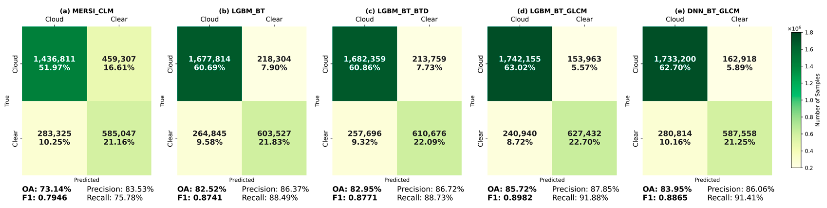
3.1. Overall Statistical Assessments

To examine the feasibility of applying LGBM and GLCM features to improve the cloud detection performance, four configurations were proposed to conduct comparative experiments. The first configuration (MERSI_CLM) is the FY-3D MERSI CLM product produced by the threshold-based algorithm, as introduced in Section 2.1. Several previous research [26,27] applied BT observations to develop random forest models, which provided accurate cloud detection data. Thus, the second (LGBM_BT) is an LGBM model trained using the brightness temperature (BT) observations of the six thermal channels. Besides BT, BT difference (BTD) values were also employed as useful input variables of ensemble tree models to retrieve clouds [16,29]. In addition to BT, the third configuration (LGBM_BT_BTD) involved 15 BTD to train an LGBM model. LGBM_BT_GLCM employed both 6 BT and the corresponding 96 GLCM features to produce an LGBM model. Last, the baseline DNN model (DNN_BT_GLCM) with the same inputs of LGBM_BT_GLCM was produced for comparison. A detailed analysis of the proposed algorithm’s ability to further analysis was carried out to provide a comprehensive quantitative assessment of cloud detection across various scenarios, including variations in solar zenith angles, surface types, cloud layer numbers, and cloud top altitudes in Section 3.2, Section 3.3 and Section 3.4. The accuracy assessment of cloud detection was performed based on the collocated dataset of 2021.

The detailed quantitative accuracy evaluation results for the cloud detection are presented in Figure 1. From the figure, it is evident that LGBM_BT_GLCM achieves the highest OA and F1 values among all the configurations. Compared to the traditional threshold-based method (MERSI_CLM), the implementation of the LGBM algorithm with only BT (i.e., LGBM_BT) significantly enhances the cloud detection performance during nighttime, resulting in an increase in OA from 73.14% to 82.52%. Especially noteworthy is the 12.71% improvement in the recall metric (MERSI_CLM: 75.78%; LGBM_BT: 88.49%). Among these models, the precision improves progressively with the inclusion of additional features, increasing from 83.53% (MERSI_CLM) to 87.85% (LGBM_BT_GLCM). Concurrently, both the FP and FN rates exhibit a decreasing trend, indicating that the detection performance becomes more robust and less prone to confusion as more features are incorporated. Notably, the highest FN rate is observed in MERSI_CLM and DNN_BT_GLCM, suggesting that these two models are less effective at identifying cloud pixels accurately compared to other models. The recall represents how well the algorithm captures all instances of clouds, indicating its effectiveness in not missing any clouds during the detection process. Therefore, more clouds can be detected accurately through the utilization of the LGBM during nighttime. Nevertheless, LGBM_BT and LGBM_BT_BTD produced comparable results across all metrics. With the utilization of GLCM features, the LGBM model (LGBM_BT_GLCM) demonstrated improvements of 3.20% in OA, 0.0241 in F1, and 3.39% in recall compared to LGBM_BT. However, DNN_BT_GLCM produced lower metrics (OA: 83.95%, F1:0.8865) compared to LGBM_BT_GLCM. Thus, the following evaluations only focus on the operational product algorithm (MERSI_CLM) and LGBM-based models.

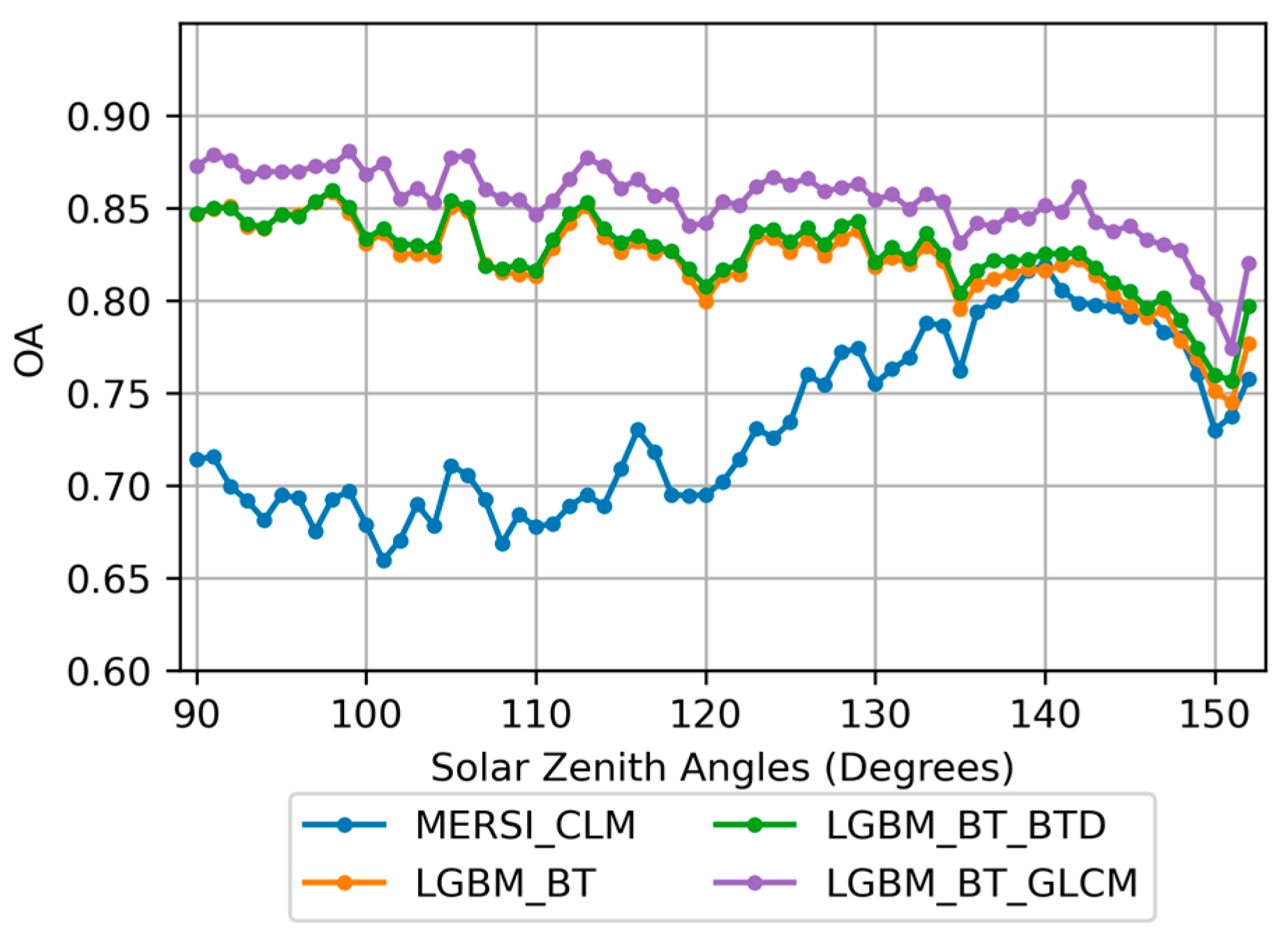
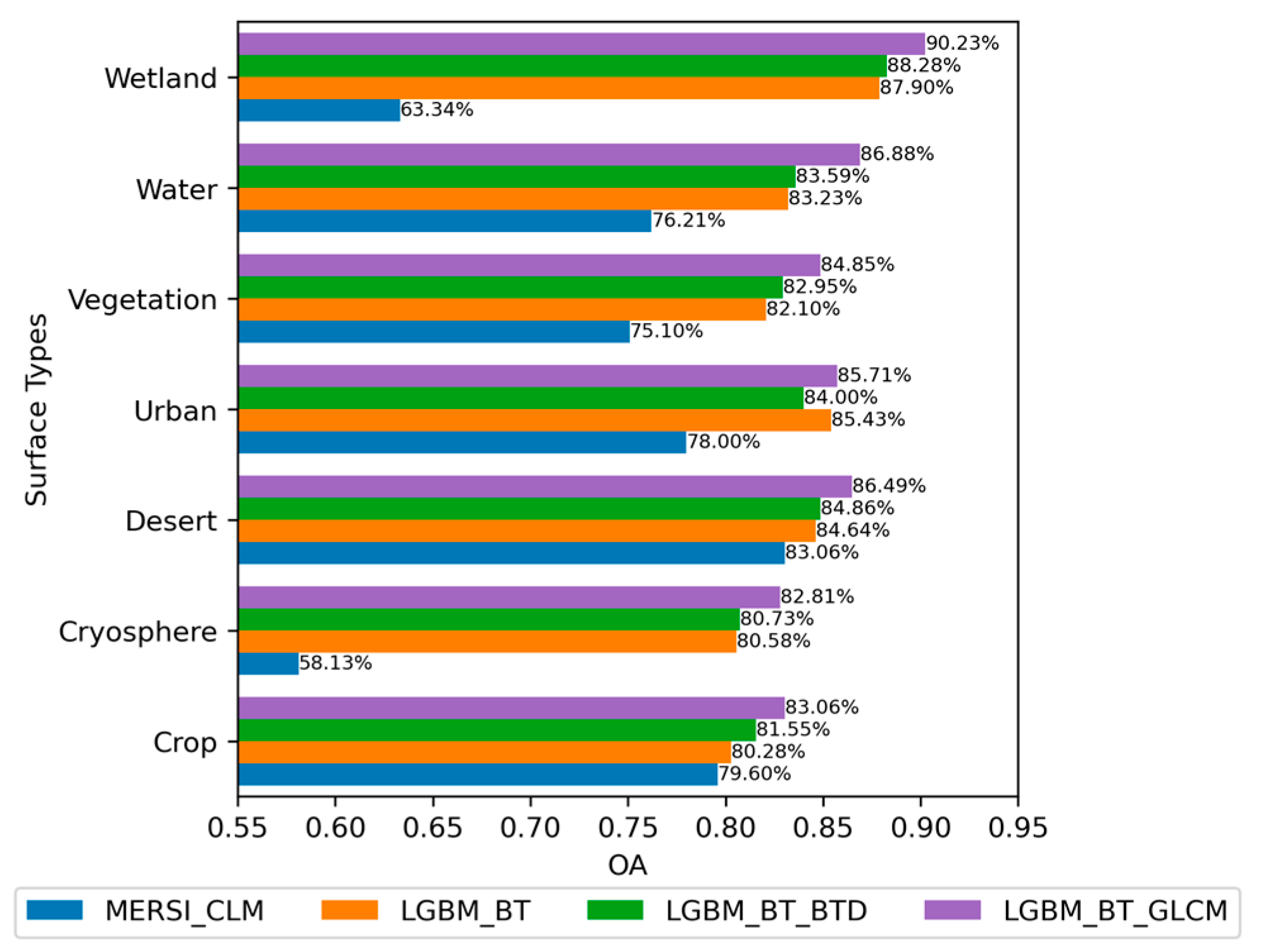
3.2. Cloud Detection Evaluations by Solar Zenith Angles and Surface Types

The assessment of cloud detection for the four configurations across solar zenith angles was investigated. Figure 2 presents OA in each 1-degree bin of solar zenith angles from 90 to 153 degrees. Across the range of solar zenith angles, LGBM_BT_GLCM consistently outperforms the other three configurations. Especially evident in Figure 2, when solar zenith angles are below 125 degrees, LGBM_BT_GLCM achieved over 85% OA in nearly all categories. It is worth noting that the overall accuracy of all configurations has declined, with solar zenith angles exceeding 140 degrees. On the one hand, solar zenith angles indicate the temporal information of the imagery observations captured. Polar-orbiting satellites like FY-3D and CALIPSO record the solar zenith angle at each observation pixel with the surface as the coordinate system. A 0-degree angle represents midday, a 90-degree angle represents sunrise or sunset, and a 180-degree angle theoretically indicates the sun located on the opposite side of the Earth (i.e., midnight). As the solar zenith angle increases from 90 degrees, the time moves further towards deep night. During the night, clouds may appear warmer compared to their surroundings due to temperature inversion occurring.

On the other hand, since FY-3D is an afternoon-orbit satellite, observations obtained during nighttime at lower solar zenith angles are generally at higher latitudes (the sub-polar and polar regions), where the surface may be covered by snow or ice. Moreover, due to the lack of solar radiation annually, the Earth’s polar areas, specifically the Arctic and Antarctic, experience significantly lower BT values compared to other regions [71]. Low contrast between clouds and snow/ice surface in BT could lead to inaccurate detection performance of MERSI_CLM at low solar zenith angles. The agreement of the findings is also indicated in Figure 3, showing that the threshold-based approach of cloud retrieval (MERSI_CLM) cannot tackle the classification difficulties in the cryosphere, thus resulting in 58.13% OA. Nevertheless, LGBM_BT_GLCM provided 82.81% OA for the cryosphere category. Moreover, in all surface types, LGBM_BT_GLCM produced the highest OA (higher than 82%) among the configurations.

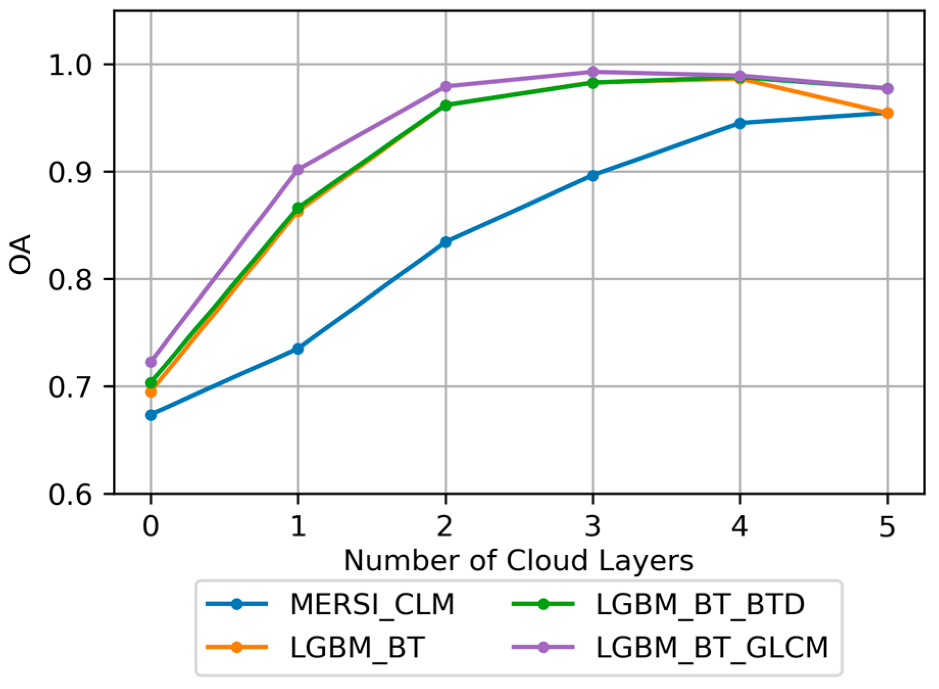
3.3. Performance of Cloud Detection with Cloud Properties

Additionally, the performance of cloud detection, along with cloud properties such as cloud top height and the number of cloud layers, was evaluated. Figure 4 depicts the comparison of OA across four configurations, with a focus on the cloud top height of the first layer. The x-axis of the figure represents cloud top heights binned at 0.5 km intervals, starting from less than 0.5 km (the bin of <0.5 km) and increasing linearly to heights beyond 10 km (the bin of >10 km). As the figure shows, the LGBM_BT_GLCM configuration outperforms the other models across the entire range of cloud top heights, except the bin of 0.5 km. LGBM_BT_GLCM emerges as the superior configuration across nearly the entire spectrum of cloud top heights. Furthermore, the three LGBM configurations exhibit a similar trend of improving OA with higher cloud top heights. Notably, within the height range of 1 to 2.5 km (bins: 1.5, 2.0, 2.5 km), LGBM_BT_GLCM outperforms the other two LGBM models by 5% to 8%. From the 2 km bin onward, LGBM_BT_GLCM consistently achieves over 90% OA, while the other two LGBM models only surpass 90% OA after the 6.5 km bin. In the first bin, spanning 0 to 0.5 km, LGBM_BT_GLCM’s OA is 3.23% lower than that of LGBM_BT_BTD. In contrast to the trends exhibited by the LGBM models, MERSI_CLM demonstrates notable fluctuations of OA across different cloud top heights. MERSI_CLM starts at approximately 48% and experiences a sharp increase as the cloud top height approaches the 2 km bin, reaching 78.42%. Following this initial rise, the OA of MERSI_CLM enters a trough, bottoming out at 67.27% at the 5.5 km bin. Afterward, the OA gradually trends upward, approaching 80% by the 8.5 km bin and reaching 87% for cloud top heights greater than 9.5 km. Overall, each algorithm exhibits varying levels of performance with respect to cloud top heights, especially in low clouds. Regarding detection accuracy, the LGBM models show less sensitivity to changes in cloud top height above 2.5 km, whereas MERSI_CLM’s OA curve takes on a distinctive bow shape, peaking at lower heights before declining and then partially recovering at higher altitudes.

Figure 5 showcases the assessment of the cloud detection performance of the four configurations across various numbers of cloud layers. The layer of 0 indicates the clear sky condition. Therefore, the accuracy at 0 indicates the precision of clear sky detection. It is observed that LGBM_BT_GLCM achieved an accuracy of 72.25% for clear sky (0 cloud layers), the highest among all configurations tested (MERSI_CLM: 67.37%; LGBM_BT: 69.50%; LGBM_BT_BTD: 70.32%). Furthermore, under cloudy conditions, LGBM_BT_GLCM demonstrated consistently high accuracies, reaching 90.18% for a single cloud layer and surpassing 97% for multiple cloud layers, thereby outperforming all other configurations. Overall, all four algorithms exhibit an improvement in their ability to detect clouds as the number of cloud layers increases. In comparison to MERSI_CLM, the implementation of LGBM enhanced accuracy by a range of 8% to 12% across cloud layers 1 to 3.

3.4. Detection Capability Under Different BT Ranges

The performance of cloud detection was investigated as a function of BT ranges at two thermal infrared channels. The observations were categorized according to BT ranging from 200 to 300 K, with each category representing a 10 K interval across two distinct channels: 3.8 and 10.8 μm. The accuracy of the model’s predictions for each BT grid is presented in Figure 6. To mitigate potential biases in the evaluation process and analysis, grids with fewer than one thousand samples were excluded, resulting in a total of 41 grids being represented in the figure. Standard deviation (SD) and expectation (E) of grid accuracy values were also computed. With comparable accuracy variation produced by the LGBM configurations, LGBM_BT_GLCM still produced the best results in nearly all grids. Moreover, LGBM_BT_GLCM provided the most robust and consistent results over the various BT ranges (E: 88.24%; SD: 7.11). On the contrary, MERSI_CLM yielded the most varied distribution of accuracies and the poorest results (E: 78.90%; SD:13.85) across the BT ranges among the configurations. In particular, the MERSI_CLM model exhibited detection accuracy in 13 grids with below 70% (six of them lower than 60%), contrasted with the LGBM models, which had just a single grid with accuracy under 70%. There are two low-accuracy regions (lower than 70%) highlighted in Figure 6a. The epicenter of Region A is pinpointed at the intersection of BT ranges between 220 and 230 K in the 3.8 µm channel and 230 and 240 K in the 10.8 um channel, providing 45.26% accuracy. Another low-accuracy region (Region B) is observed within the BT range of 280 to 290 K in the 10.8 µm channel. Figure 6 demonstrates the strengths and weaknesses of MERSI_CLM in cloud detection within certain BT ranges.

3.5. Visual Inspection Comparison

To facilitate visual inspection, two types of false-color RGB composites were generated. Various nonlinear stretching techniques were applied to BT and BT difference (BTD) data at 3.8 µm and 10.8 µm to produce nighttime RGB images (NT-RGB). These images are capable of indicating the presence of typical clouds, which are distinguishable from the surrounding surface. For the NT_RGB plots, the whiter the color, the thicker the cloud or the higher its altitude. Additionally, the TC-RGB method’s night mode, as proposed by [72], was employed to create another type of reference image. The TC-RGB method applied specific linear transformations to BTD and BT data (R: 12–10.8 µm, G: 10.8–3.8 µm, B: 10.8 µm) to generate enhanced composite imagery that highlights different cloud types and characteristics. For the TC_RGB plots, higher clouds are indicated by purple to blue, and lower clouds are indicated by fluorescent green or yellow. For thick clouds, the middle part appears ochre, while the edges transition to purple or pink.

Several examples of cloud detection results obtained using MERSI_CLM, LGBM_BT_BTD, and LGBM_BT_GLCM are presented in Figure 7 for visual inspection and comparison. Plots T1 to T3 illustrate cloud detection results over oceans. In T1, multi-layer clouds are present. MERSI_CLM successfully identified the higher clouds (indicated by purple in TC-RGB) but failed to detect the lower clouds (indicated by light yellow in TC-RGB). The lower clouds exhibit low opacity, which increases the detection difficulty. Conversely, LGBM_BT_GLCM accurately detected both types of clouds. In T2, the center of the clouds (highlighted by the red rectangle) was classified as probably clear by MERSI_CLM. T3 demonstrates a more severe false detection by MERSI_CLM, where only the cloud edges were identified, omitting the majority of the cloud body. According to TC-RGB, the undetected clouds exhibit a similar color (light yellow) in T1 to T3, indicating a specific BTD signature that the threshold-based algorithm struggles to distinguish between clouds and clear sky. Nonetheless, LGBM_BT_GLCM is able to delineate the complete cloud texture under such conditions. For the cases over land in T4, LGBM_BT_GLCM demonstrates enhanced cloud detection results compared to MERSI_CLM. Even when discriminating clouds from snow cover (T5, depicting Greenland Island), LGBM_BT_GLCM significantly outperforms MERSI_CLM.

LGBM_BT_BTD provided cloud retrieval improvements comparable to LGBM_BT_GLCM. However, as shown in T1 and T6, the cloud masks produced by LGBM_BT_BTD suffer from the effect of thermal stripes derived from the MERSI L1 imagery, introducing stripe noise, also observed in MERSI_CLM. In contrast, LGBM_BT_GLCM significantly mitigated the stripe effect, yielding more accurate cloud texture results. Furthermore, LGBM_BT_GLCM avoids the systematic error observed in MERSI_CLM (T7). Overall, upon visual inspection of the images, LGBM_BT_GLCM produced more accurate and stable cloud detection results.

3.6. Comparison to MODIS Cloud Mask Product

The MODIS cloud mask product on Aqua (MYD35_L2) was used to compare the performance of cloud detection with MERSI of LGBM_BT_GLCM. A number of threshold-based scenarios were designed to produce MYD35_L2 to indicate cloudy or clear conditions [9,10,73], which is similar to MERSI_CLM. Both Aqua and FY3D are afternoon-orbit satellites, while MERSI and MODIS provide data at the same spatial resolution of 1 km or aggregated to 1 km. The collocation of three datasets (MODIS-Aqua, FY3D-MERSI, CALIPSO-CALIOP) in 2021 was conducted, afterward generating 47,146 samples. The four MODIS cloud categories were integrated into binary labels (cloudy, clear). The capability of cloud detection by the two products was evaluated by the CALIOP L2 product.

Figure 8 presents the statistical assessment results of MYD35_L2 and LGBM_BT_GLCM. The proposed algorithm produced 90.30% OA and 0.9397 F1 higher than MYD35_L2 by 5.64% OA and 0.0394 F1. Specifically, the precision scores of the two products are comparable, whereas the recall of LGBM_BT_GLCM is significantly higher than that of MYD35_L2 by 7.53%. Therefore, it demonstrates that the cloud retrieval capability of the proposed model exhibits a significant improvement compared to MYD35_L2.

In the same way as the visual inspection method in 4.2, three examples are shown in Figure 9. Since the collocation between MYD35_L2 and LGBM_BT_GLCM datasets remains a geocoordinate difference to some extent, every plot in Figure 9 is projected to an orthographic projection system. Overall, neither result shows significant differences in the identification of cloud areas, including thick and thin clouds in various altitudes. But, MYD35_L2 displays a stricter cloud detection result, which marks large amounts of suspicious pixels as probably clear. LGBM_BT_GLCM performed rather stable when the underlying surface contains BT (or BTD) gradient field, especially in T3, when the sea displays an ununiform surface, and MYD35_L2 detects the boundary as clouds or probable clouds, whereas LGBM_BT_GLCM does not.

4. Discussion

4.1. Cloud Detection Enhancements by Applying the Proposed Methodology

According to the statistical assessment results in Section 3.1, applying LGBM enhances the accuracy of cloud detection compared to the traditional threshold-based method in three aspects: (a) twilight hours, (b) cryosphere covers, and (c) limited thermal bands. During twilight hours, the significant uncertainties inherent in observations caused by scattering, spanning from visible to mid-wave infrared channels, raise severe issues regarding cloud detection. The noises in the shorter wavelength thermal bands introduce much more uncertainties in the cloud detection results produced by MERSI_CLM. Additionally, the LGBM models exhibit superior OA in the presence of ice or snow cover on the surface. Discriminating between clouds and cryosphere categories is challenging because of small thermal BT contrasts. The inadequate capability of cloud detection by using threshold-based algorithms above the cryosphere has been noted in several preceding studies [19,74,75]. Moreover, in polar regions, the occurrence of temperature inversion phenomena creates further complexities in cloud detection. In extreme conditions, such as during the deep polar night, it can occur that even high-altitude clouds are warmer than the Earth’s surface [10,14]. This inversion of temperature poses significant challenges for cloud detection and characterization, as it defies the typical thermal gradient expected in atmospheric conditions, making it nearly impossible to distinguish clouds from clear skies using threshold-based algorithms [14]. Compared to MODIS, MERSI does not carry with the three thermal bands (6.7, 13.935, 14.235 µm) significant to cloud detection [9,10,11,14]. The 6.7 µm band is typically associated with the absorption of water vapor. It has been used as a crucial input for the development of cloud detection algorithms [9,10,11,14]. In particular, the 6.7 µm radiation emanating around the 600 hPa level is reliably detected by the sensors, whereas the radiation originating from lower clouds or the Earth’s surface is absorbed in the atmosphere [76], thus having not been reflected in the imagery. Therefore, the use of BT at 6.7 µm is beneficial to detect the presence of clouds around 600 hPa. As illustrated in Figure 4, the absence of 6.7 µm data might influence the accuracy of MERSI_CLM in the detection of clouds with top heights ranging from 3.5 km to 5.5 km. Moreover, the 6.7 µm band was also used to cope with the effect of temperature inversion for cloud detection [76]. The other CO₂ slicing bands (13.935 and 14.235 µm) were used to conduct cloud mask detection. The use of the 13.935 band had primarily been designed to detect thick clouds at high altitudes [9]. Furthermore, the 14.235 µm band was involved in the framework to improve the capability to identify clouds over the Antarctic plateau under very cold conditions [14]. LGBM is used to find data representations that can serve as proxies for the missing thermal bands. Meanwhile, the model can learn complex patterns and relationships that are indicative of cloud presence from the MERSI thermal bands. Thus, while the lack of specific thermal bands in MERSI data poses challenges for cloud detection, the application of LGBM can significantly mitigate these challenges. By leveraging the model’s capabilities in handling limited thermal information, learning complex data representations, and adapting to the data’s characteristics, it is possible to provide promising cloud mask data during nighttime.

The improvements of at least 2~3% OA in all evaluation aspects compared to non-GLCM models indicate that incorporating GLCM is beneficial to enhance the nighttime cloud detection capability of LGBM for MERSI L1. Notably, for the clouds with 1 to 2.5 km altitudes, LGBM_BT_GLCM significantly shows a stronger detection performance, achieving higher precision and recall rates. This suggests that the texture features captured by GLCM provide crucial information that aids in distinguishing clouds from other atmospheric phenomena, especially at these specific altitudes. Additionally, LGBM_BT_GLCM is also able to alleviate the effect of thermal stripes originating from the L1 data. Electronic crosstalk results in degradation of image quality [77,78], which easily occurs in optical remote sensing sensors. The stripe noise in thermal infrared bands also significantly affects the quality of cloud detection [79] since the algorithm heavily relies on accurate BT values. Nevertheless, GLCM can reduce stripe noise because it enhances texture analysis, leading to more reliable BT measurements. By GLCM, which can be interpreted as joint grey-level probability density distributions or 2-D image histograms, the method reduces the sensitivity to image contrast and focuses on spatial relationships between pixel intensities [53]. This approach allows for more accurate differentiation between actual thermal patterns and noise artifacts.

4.2. Variable Importance

To demonstrate the contribution and usage of input variables to the retrieval task in LGBM_BT_GLCM, the analysis of variable importance was also conducted. The importance was computed during model training, indicating the frequency of feature usage in the model. The importance values were normalized to [0, 1]. Figure 10 presents the top 20 variables and the corresponding importance values. The top 6 highlighted in red are BT variables, thus indicating that the spectral information still predominately makes more contribution to the model development compared to the GLCM features. BT22, the most influential variable in the ranking, is a water vapor channel centered at a wavelength of 7.2 µm. This thermal band is a crucial element for enhancing the detection of nighttime clouds in polar regions for the MODIS cloud mask product [10,14]. The BT difference between 7.2 µm and 11 µm is sensitive to the low atmosphere in clear sky conditions, while under cloudy skies, the BT difference between 7.2 µm and 11 µm is relatively smaller than that in clear skies. The occurrence of low clouds over the Arctic and Antarctic areas at night may result in the formation of a temperature inversion; in such a situation, the 7.2 µm band provides important sensitivity to low clouds together with the 11 µm band. Shortwave bands (BT20 and BT21) are also helpful since, for some ecosystems, the change in surface emissivity within the shortwave infrared spectrum is significantly less than that in longwave bands, whereas the variation in cloud emissivity across this spectrum is still considerable [9]. Moreover, BT of shortwave infrared is also influenced by cloud optical depth and particle size, particularly in the case of ice clouds, due to the scattering of radiation [14]. Meanwhile, for longwave infrared channels, the absorption of ice and water vapor increases as one moves beyond 10.5 µm, albeit at varying rates [9]. Therefore, shortwave thermal infrared bands, associated with longwave bands (>8 µm), were employed to identify the presence of clouds. Utilizing these bands is beneficial for the detection of thin clouds and clouds above oceans. In summary, the water vapor-related band (BT22, 7.20 µm), unique in its placement outside the standard atmospheric transparency windows, plays a pivotal role in constructing the LGBM_BT_GLCM model. This is consistent with the findings in previous research [46,48], which illustrate a comparable level of importance for thermal bands in cloud-related retrieval tasks using ensemble tree models.

In terms of the GLCM variables, COR emerges as a particularly prominent and influential variable in the model generation process for cloud detection. COR is adept at capturing the linear interdependencies between pixel values within a local spatial context, such as the 7 × 7-pixel neighborhood examined in this study. Clouds, with their unique textural attributes, can be effectively distinguished from the surrounding terrain due to their typically uniform texture, which often translates into a strong positive correlation within the GLCM analysis. In contrast, the COR values tend to be lower for more heterogeneous or complex surfaces, reflecting their greater variability in pixel values.

Moreover, by averaging the correlation across the 7 × 7-pixel patch, the metric becomes more robust against random noise and isolated outliers that might be present in the imagery. This noise reduction enhances the overall accuracy of cloud detection algorithms by focusing on the consistent patterns that characterize cloud cover rather than the anomalies that can distort the picture at the pixel level. Consequently, COR’s efficacy in capturing cloud textures and edges makes it an indispensable component in the development of sophisticated models for interpreting MERSI data and improving the detection of clouds from spaceborne observations.

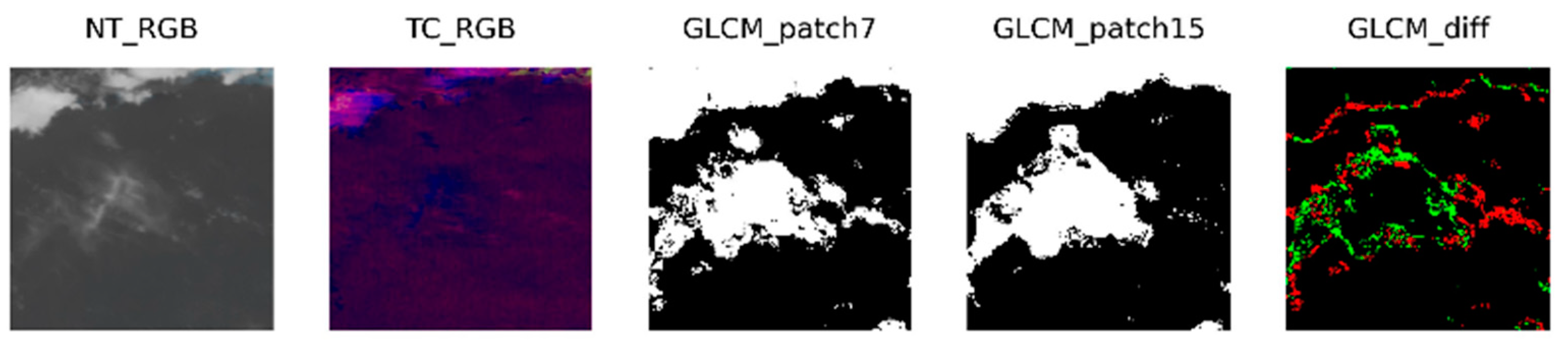
4.3. Practice of GLCM Parameters

As previously discussed, GLCM, as a useful descriptor of imagery texture, has been widely applied in numerous retrieval tasks within the field of remote sensing. In recent years, GLCM measures have been increasingly considered valuable input variables for machine learning algorithms, enhancing their retrieval capabilities. Although many studies have empirically determined GLCM parameters (patch size, distance, grey levels), few have systematically evaluated the impact of these parameters on retrieval task effectiveness. This gap hinders optimal parameter selection for improved performance.

Table 6. Comparison of overall accuracy and F1 score across various GLCM patch sizes (first column) and distance parameters (first row). (Bold: the two best results).

OA/F1	1	2	3	4	5
3 × 3	84.60%/0.8902	84.60%/0.8902	-	-	-
7 × 7	85.69%/0.8980	85.65%/0.8977	85.59%/0.8974	-	-
15 × 15	86.19%/0.9012	86.12%/0.9006	86.05%/0.9003	86.07%/0.9004	86.14%/0.9009
31 × 31	85.99%/0.8997	85.97%/0.8995	85.92%/0.8993	85.90%/0.8991	85.87%/0.8989

resents the comparison of nighttime cloud detection performance, measured by OA and F1, across various patch sizes and distances. As the patch size was increased from 3 × 3 to 15 × 15, there was a further improvement in both OA and F1 of cloud detection. However, the patch size of 31 × 31 leads to decreased performance compared to 15 × 15. Additionally, for each patch size, the evaluation metrics are comparable across different distances.

The patch size determines the amount of information to be captured and described. Small patch sizes often fail to extract adequate information to perform an accurate analysis due to high within-class heterogeneity [68]. Conversely, applying larger patch sizes yields more uniform GLCM measure values of intra-class, offering more homogeneous and better separable characterizations of the types [80]. However, excessively large patch sizes may overlap with different classes, introducing confusing spatial information and causing blurring effects between adjacent classes, referred to as the edge effect [80,81,82]. The optimal patch size also depends on the spatial resolution of the imagery. Processing higher spatial resolution data, in general, requires a larger patch size than a coarser one due to the increased heterogeneity of earth observation objects in finer-resolution imagery [83]. In this research, the patch size affects the cloud interpretation of MERSI images with a 1 km resolution by the algorithm. As illustrated in Figure 11, for cloud objects, patch 15 exhibits more pronounced edge effects compared to patch 7, leading to cloud overestimation at the margins. The last plot highlights the classification differences between the two patch sizes. Green represents pixels of clear sky mis-detected by patch 15 to clouds but not by patch 7, indicating sever blurring raised by patch 15. On the other hand, red pixels show that patch 7 effectively delineates broken clouds, which patch 15 fails to detect. Therefore, the optimal patch size is a compromise between high overall accuracy and maintaining a small enough patch so as to alleviate the edge effect [84]. Patch 7 was ultimately selected for this research. Distance refers to the pixel offset used to define the spatial relationship between pixel pairs. By default, this is set to one inter-pixel distance, which corresponds to the image’s spatial resolution. However, if the patch size is sufficiently large, employing a larger offset could be preferable. Based on the results of Table 6 the distance does not affect the effeteness of the GLCM variable calculation. A distance of 1 was used in this research.

Before calculating the GLCM matrix, images with floating-point BT values (32 bits) should be quantized to a specific number of grey levels (integers).

Table 7. Comparison of evaluation scores across different grey levels. (Bold: the best result).

Metrics	4-Bits	5-Bits	6-Bits	7-Bits	8-Bits
OA	83.35%	83.96%	84.59%	85.09%	85.69%
F1	0.8814	0.8858	0.8902	0.8938	0.8980
Precision	86.02%	86.43%	86.85%	87.21%	87.82%
Recall	76.51%	90.83%	91.31%	91.67%	91.87%

resents the cloud detection results using a 7 × 7 window size and a distance of 1 across different grey levels. The best results were achieved with 8-bit images (256 grey levels), whereas 4-bit images (16 grey levels) performed the poorest. High grey levels are often preferred to capture fine details, leading to better diagnostic capabilities. The 7- and 8-bit quantization methods show practically the same evaluation scores across different gray levels. This similarity is due to the minimal quantization error and the robustness of GLCM texture features to small variations in pixel intensity values. Practical considerations such as memory, processing power, and time constraints arise with higher grey levels. For instance, processing the same number of MERSI observations with 128 grey levels (7 bits) takes half the time of 256 grey levels. Thus, real-time processing tasks may prefer lower grey levels. To demonstrate the optimal performance of the proposed framework, 256 grey levels (8 bits) were eventually applied.

4.4. Limitations

The primary limitation of the study stems from the constraints imposed by the collocated datasets of MODIS and CALIOP for cloud detection. With a maximum matching distance of 1 km and a temporal gap of 15 min, there arises a potential for uncertainty within the analysis. Complicating matters further, the operational trajectory of CALIOP often spans across two sides of MERSI images, resulting in observations susceptible to the bow tie effect, thereby lowering their quality. This inherent disparity makes accurate comparison and interpretation of data between the two satellite platforms challenging. Consequently, the factors influencing cloud mask retrieval remain unexamined within this study. Compared to point-by-point threshold-based algorithms, using GLCM in the proposed method overestimates the edge of large clouds and omits a few small-scale broken clouds covering 1–4 pixels. These misclassifications slightly affect the accuracy of the current study. Moreover, in the absence of ample optical information during nighttime, manual interpretation and inspection heavily rely on false color RGB composites derived from thermal infrared channels. This reliance introduces a layer of visual ambiguity, particularly in distinguishing subtle phenomena like thin clouds from atmospheric elements such as water vapor and aerosols, potentially skewing the analysis. Hence, further analysis could benefit from incorporating additional sources of ground truth data to assess cloud detection performance, such as CloudSAT CPR, GPM DPR, and land-based radar observations. Expanding the dataset in this manner would provide a more comprehensive evaluation of cloud detection accuracy and enhance the robustness of the study’s findings.

5. Conclusions

The study’s primary objective was to enhance cloud detection performance in optical remote sensing imagery by leveraging LGBM models with GLCM features. Our comprehensive evaluation of four distinct configurations, MERSI_CLM, LGBM_BT, LGBM_BT_BTD, and LGBM_BT_GLCM, demonstrates that the integration of GLCM features significantly boosts detection accuracy and robustness.

The LGBM_BT_GLCM model outperformed other configurations across all evaluated metrics, achieving the highest OA (85.69%) and F1 (0.898). This model also showed a notable improvement in recall by 3.39% compared to the LGBM_BT model, indicating its superior ability to correctly identify cloudy pixels. The LGBM_BT_GLCM model consistently maintained high accuracy across various BT ranges, with the lowest standard deviation (7.11) and highest expectation (88.24%). Under different cloudy conditions, LGBM_BT_GLCM demonstrated consistently high accuracies, reaching 90.18% for a single cloud layer and surpassing 97% for multiple cloud layers. The LGBM_BT_GLCM model exhibited exceptional performance across diverse surface types, including challenging environments such as snow-covered regions, where it achieved an overall accuracy exceeding 82.81%. This highlights its adaptability and reliability in complex scenarios where traditional methods often struggle. Visual inspections using false-color RGB composites corroborated the statistical findings, with the LGBM_BT_GLCM model providing more stable and accurate cloud detection results, effectively mitigating issues like thermal stripes and misclassifications seen in other models. For cloud top heights of 2 km and above, the LGBM_BT_GLCM model consistently achieves over 90% OA, avoiding the accuracy loss observed in MERSI_CLM when detecting clouds with top heights ranging from 3.5 km to 5.5 km. Even with the absence of several thermal bands available to MODIS, the LGBM_BT_GLCM model demonstrates that it can achieve comparable performance in cloud detection from MERSI, achieving an overall accuracy of 90.30% and an F1-Score of 0.9397. The integration of GLCM features into the LGBM framework not only compensates for the lack of thermal bands but also enhances the model’s overall detection accuracy and robustness. This comparison underscores the potential of advanced machine learning techniques to meet and even exceed the capabilities of traditional satellite-based cloud detection methods. Moreover, compared to the baseline deep learning model DNN_BT_GLCM, the LGBM_BT_GLCM framework achieves higher accuracy and computational efficiency, making it more suitable for large-scale satellite data training where manual labeling is challenging.

The integration of spatial features into LGBM models represents a promising advancement in the field of cloud detection. Furthermore, the incorporation of temporal information into ML algorithms for cloud detection is a valuable area for further exploration, especially for geostationary satellite data. In conclusion, the LGBM_BT_GLCM model’s superior performance, particularly in challenging detection scenarios, underscores its potential to enhance satellite-based cloud monitoring and contribute to more accurate weather and climate analysis.

References

1. Stephens, G.L. Cloud Feedbacks in the Climate System: A Critical Review. J. Clim. 2005, 18, 237–273. [Google Scholar] [CrossRef]
2. Baker, M.B.; Peter, T. Small-scale cloud processes and climate. Nature 2008, 451, 299–300. [Google Scholar] [CrossRef] [PubMed]
3. Bengtsson, L. The global atmospheric water cycle. Environ. Res. Lett. 2010, 5, 2. [Google Scholar] [CrossRef]
4. Fernández-Prieto, D.; van Oevelen, P.; Su, Z.; Wagner, W. Editorial “Advances in Earth observation for water cycle science”. Hydrol. Earth Syst. Sci. 2012, 16, 543–549. [Google Scholar] [CrossRef]
5. Huang, J.; Lin, C.; Li, Y.; Huang, B. Effects of humidity, aerosol, and cloud on subambient radiative cooling. Int. J. Heat Mass Transf. 2022, 186, 122438. [Google Scholar] [CrossRef]
6. King, M.D.; Platnick, S.; Menzel, W.P.; Ackerman, S.A.; Hubanks, P.A. Spatial and Temporal Distribution of Clouds Observed by MODIS Onboard the Terra and Aqua Satellites. IEEE Trans. Geosci. Remote Sens. 2013, 51, 3826–3852. [Google Scholar] [CrossRef]
7. Stubenrauch, C.J.; Rossow, W.B.; Kinne, S.; Ackerman, S.; Cesana, G.; Chepfer, H.; Di Girolamo, L.; Getzewich, B.; Guignard, A.; Heidinger, A.; et al. Assessment of Global Cloud Datasets from Satellites: Project and Database Initiated by the GEWEX Radiation Panel. Bull. Am. Meteorol. Soc. 2013, 94, 1031–1049. [Google Scholar] [CrossRef]
8. Zhang, B.; Guo, Z.; Zhang, L.; Zhou, T.; Hayasaka, T. Cloud Characteristics and Radiation Forcing in the Global Land Monsoon Region From Multisource Satellite Data Sets. Earth Space Sci. 2020, 7, e2019EA001027. [Google Scholar] [CrossRef]
9. Ackerman, S.A.; Strabala, K.I.; Menzel, W.P.; Frey, R.A.; Moeller, C.C.; Gumley, L.E. Discriminating clear sky from clouds with MODIS. J. Geophys. Res. Atmos. 1998, 103, 32141–32157. [Google Scholar] [CrossRef]
10. Frey, R.A.; Ackerman, S.A.; Liu, Y.; Strabala, K.I.; Zhang, H.; Key, J.R.; Wang, X. Cloud Detection with MODIS. Part I: Improvements in the MODIS Cloud Mask for Collection 5. J. Atmos. Ocean. Technol. 2008, 25, 1057–1072. [Google Scholar] [CrossRef]
11. Platnick, S.; King, M.D.; Ackerman, S.A.; Menzel, W.P.; Baum, B.A.; Riédi, J.C.; Frey, R.A. The MODIS cloud products: Algorithms and examples from terra. IEEE Trans. Geosci. Remote Sens. 2003, 41, 459–473. [Google Scholar] [CrossRef]
12. Ackerman, S.A.; Holz, R.E.; Frey, R.; Eloranta, E.W.; Maddux, B.C.; McGill, M. Cloud Detection with MODIS. Part II: Validation. J. Atmos. Ocean. Technol. 2008, 25, 1073–1086. [Google Scholar] [CrossRef]
13. Liu, Y.; Ackerman, S.A.; Maddux, B.C.; Key, J.R.; Frey, R.A. Errors in Cloud Detection over the Arctic Using a Satellite Imager and Implications for Observing Feedback Mechanisms. J. Clim. 2010, 23, 1894–1907. [Google Scholar] [CrossRef]
14. Liu, Y.; Key, J.R.; Frey, R.A.; Ackerman, S.A.; Menzel, W.P. Nighttime polar cloud detection with MODIS. Remote Sens. Environ. 2004, 92, 181–194. [Google Scholar] [CrossRef]
15. Maddux, B.C.; Ackerman, S.A.; Platnick, S. Viewing Geometry Dependencies in MODIS Cloud Products. J. Atmos. Ocean. Technol. 2010, 27, 1519–1528. [Google Scholar] [CrossRef]
16. Liu, C.; Yang, S.; Di, D.; Yang, Y.; Zhou, C.; Hu, X.; Sohn, B.-J. A Machine Learning-based Cloud Detection Algorithm for the Himawari-8 Spectral Image. Adv. Atmos. Sci. 2021, 39, 1994–2007. [Google Scholar] [CrossRef]
17. Irish, R.R.; Barker, J.L.; Goward, S.N.; Arvidson, T. Characterization of the Landsat-7 ETM+ Automated Cloud-Cover Assessment (ACCA) Algorithm. Photogramm. Eng. Remote Sens. 2006, 72, 1179–1188. [Google Scholar] [CrossRef]
18. Karpatne, A.; Jiang, Z.; Vatsavai, R.R.; Shekhar, S.; Kumar, V. Monitoring Land-Cover Changes: A Machine-Learning Perspective. IEEE Geosci. Remote Sens. Mag. 2016, 4, 8–21. [Google Scholar] [CrossRef]
19. Ishida, H.; Oishi, Y.; Morita, K.; Moriwaki, K.; Nakajima, T.Y. Development of a support vector machine based cloud detection method for MODIS with the adjustability to various conditions. Remote Sens. Environ. 2018, 205, 390–407. [Google Scholar] [CrossRef]
20. Wang, Q.; Zhou, C.; Zhuge, X.; Liu, C.; Weng, F.; Wang, M. Retrieval of cloud properties from thermal infrared radiometry using convolutional neural network. Remote Sens. Environ. 2022, 278, 113079. [Google Scholar] [CrossRef]
21. Tao, R.; Zhang, Y.; Wang, L.; Liu, Q.; Wang, J. U-High resolution network (U-HRNet): Cloud detection with high-resolution representations for geostationary satellite imagery. Int. J. Remote Sens. 2021, 42, 3511–3533. [Google Scholar] [CrossRef]
22. Tuia, D.; Kellenberger, B.; P’erez-Suay, A.; Camps-Valls, G. A Deep Network Approach to Multitemporal Cloud Detection. In Proceedings of the International Geoscience and Remote Sensing Symposium (IGARSS), Valencia, Spain, 22–27 July 2018. [Google Scholar]
23. Li, X.; Yang, X.; Li, X.; Lu, S.; Ye, Y.; Ban, Y. GCDB-UNet: A novel robust cloud detection approach for remote sensing images. Knowl.Based Syst. 2022, 238, 107890. [Google Scholar] [CrossRef]
24. Zhao, C.; Zhang, X.; Kuang, N.; Luo, H.; Zhong, S.; Fan, J. Boundary-Aware Bilateral Fusion Network for Cloud Detection. IEEE Trans. Geosci. Remote Sens. 2023, 61, 5403014. [Google Scholar] [CrossRef]
25. Li, J.; Hu, C.; Sheng, Q.; Wang, B.; Ling, X.; Gao, F.; Xu, Y.; Li, Z.; Molinier, M. A Unified Cloud Detection Method for Suomi-NPP VIIRS Day and Night PAN Imagery. IEEE Trans. Geosci. Remote Sens. 2024, 62, 4106913. [Google Scholar] [CrossRef]
26. Gomis-Cebolla, J.; Jimenez, J.C.; Sobrino, J.A. MODIS probabilistic cloud masking over the Amazonian evergreen tropical forests: A comparison of machine learning-based methods. Int. J. Remote Sens. 2019, 41, 185–210. [Google Scholar] [CrossRef]
27. Wang, C.; Platnick, S.; Meyer, K.; Zhang, Z.; Zhou, Y. A machine-learning-based cloud detection and thermodynamic-phase classification algorithm using passive spectral observations. Atmos. Meas. Tech. 2020, 13, 2257–2277. [Google Scholar] [CrossRef]
28. Fu, H.; Shen, Y.; Liu, J.; He, G.; Chen, J.; Liu, P.; Qian, J.; Li, J. Cloud Detection for FY Meteorology Satellite Based on Ensemble Thresholds and Random Forests Approach. Remote Sens. 2018, 11, 44. [Google Scholar] [CrossRef]
29. Yang, Y.; Sun, W.; Chi, Y.; Yan, X.; Fan, H.; Yang, X.; Ma, Z.; Wang, Q.; Zhao, C. Machine learning-based retrieval of day and night cloud macrophysical parameters over East Asia using Himawari-8 data. Remote Sens. Environ. 2022, 273, 112971. [Google Scholar] [CrossRef]
30. Ke, G.; Meng, Q.; Finley, T.; Wang, T.; Chen, W.; Ma, W.; Ye, Q.; Liu, T.Y. LightGBM: A highly efficient gradient boosting decision tree. In Proceedings of the 31st International Conference on Neural Information Processing Systems, Long Beach, CA, USA, 4–9 December 2017. [Google Scholar]
31. Dong, L.; Qi, J.; Yin, B.; Zhi, H.; Li, D.; Yang, S.; Wang, W.; Cai, H.; Xie, B. Reconstruction of Subsurface Salinity Structure in the South China Sea Using Satellite Observations: A LightGBM-Based Deep Forest Method. Remote Sens. 2022, 14, 3494. [Google Scholar] [CrossRef]
32. Su, H.; Lu, X.; Chen, Z.; Zhang, H.; Lu, W.; Wu, W. Estimating Coastal Chlorophyll-A Concentration from Time-Series OLCI Data Based on Machine Learning. Remote Sens. 2021, 13, 576. [Google Scholar] [CrossRef]
33. Xiang, L.; Xu, Y.; Sun, H.; Zhang, Q.; Zhang, L.; Zhang, L.; Zhang, X.; Huang, C.; Zhao, D. Retrieval of Subsurface Velocities in the Southern Ocean from Satellite Observations. Remote Sens. 2023, 15, 5699. [Google Scholar] [CrossRef]
34. Ji, X.; Ma, Y.; Zhang, J.; Xu, W.; Wang, Y. A Sub-Bottom Type Adaption-Based Empirical Approach for Coastal Bathymetry Mapping Using Multispectral Satellite Imagery. Remote Sens. 2023, 15, 3570. [Google Scholar] [CrossRef]
35. Lin, S.; Chen, N.; He, Z. Automatic Landform Recognition from the Perspective of Watershed Spatial Structure Based on Digital Elevation Models. Remote Sens. 2021, 13, 3926. [Google Scholar] [CrossRef]
36. Bui, Q.-T.; Chou, T.-Y.; Hoang, T.-V.; Fang, Y.-M.; Mu, C.-Y.; Huang, P.-H.; Pham, V.-D.; Nguyen, Q.-H.; Anh, D.T.N.; Pham, V.-M.; et al. Gradient Boosting Machine and Object-Based CNN for Land Cover Classification. Remote Sens. 2021, 13, 2709. [Google Scholar] [CrossRef]
37. Sevgen, E.; Abdikan, S. Classification of Large-Scale Mobile Laser Scanning Data in Urban Area with LightGBM. Remote Sens. 2023, 15, 3787. [Google Scholar] [CrossRef]
38. Sang, M.; Xiao, H.; Jin, Z.; He, J.; Wang, N.; Wang, W. Improved Mapping of Regional Forest Heights by Combining Denoise and LightGBM Method. Remote Sens. 2023, 15, 5436. [Google Scholar] [CrossRef]
39. Chai, X.; Li, J.; Zhao, J.; Wang, W.; Zhao, X. LGB-PHY: An Evaporation Duct Height Prediction Model Based on Physically Constrained LightGBM Algorithm. Remote Sens. 2022, 14, 3448. [Google Scholar] [CrossRef]
40. Sun, Y.; Zhang, F.; Lin, H.; Xu, S. A Forest Fire Susceptibility Modeling Approach Based on Light Gradient Boosting Machine Algorithm. Remote Sens. 2022, 14, 4362. [Google Scholar] [CrossRef]
41. Xiong, P.; Long, C.; Zhou, H.; Battiston, R.; Zhang, X.; Shen, X. Identification of Electromagnetic Pre-Earthquake Perturbations from the DEMETER Data by Machine Learning. Remote Sens. 2020, 12, 3643. [Google Scholar] [CrossRef]
42. Yang, Z.; He, Q.; Miao, S.; Wei, F.; Yu, M. Surface Soil Moisture Retrieval of China Using Multi-Source Data and Ensemble Learning. Remote Sens. 2023, 15, 2786. [Google Scholar] [CrossRef]
43. Wang, Q.; Zhou, C.; Letu, H.; Zhu, Y.; Zhuge, X.; Liu, C.; Weng, F.; Wang, M. Obtaining Cloud Base Height and Phase from Thermal Infrared Radiometry Using a Deep Learning Algorithm. IEEE Trans. Geosci. Remote Sens. 2023, 61, 4105914. [Google Scholar] [CrossRef]
44. Zhuge, X.; Zou, X.; Wang, Y. Determining AHI Cloud-Top Phase and Intercomparisons with MODIS Products Over North Pacific. IEEE Trans. Geosci. Remote Sens. 2021, 59, 436–448. [Google Scholar] [CrossRef]
45. Wang, X.; Iwabuchi, H.; Yamashita, T. Cloud identification and property retrieval from Himawari-8 infrared measurements via a deep neural network. Remote Sens. Environ. 2022, 275, 113026. [Google Scholar] [CrossRef]
46. Min, M.; Li, J.; Wang, F.; Liu, Z.; Menzel, W.P. Retrieval of cloud top properties from advanced geostationary satellite imager measurements based on machine learning algorithms. Remote Sens. Environ. 2020, 239, 111616. [Google Scholar] [CrossRef]
47. Tan, Z.; Huo, J.; Ma, S.; Han, D.; Wang, X.; Hu, S.; Yan, W. Estimating cloud base height from Himawari-8 based on a random forest algorithm. Int. J. Remote Sens. 2020, 42, 2485–2501. [Google Scholar] [CrossRef]
48. Yu, Z.; Ma, S.; Han, D.; Li, G.; Gao, D.; Yan, W. A cloud classification method based on random forest for FY-4A. Int. J. Remote Sens. 2021, 42, 3353–3379. [Google Scholar] [CrossRef]
49. Zhang, C.; Zhuge, X.; Yu, F. Development of a high spatiotemporal resolution cloud-type classification approach using Himawari-8 and CloudSat. Int. J. Remote Sens. 2019, 40, 6464–6481. [Google Scholar] [CrossRef]
50. Haralick, R.M. Statistical and Structural Approaches to Texture. Proc. IEEE 1979, 67, 786–804. [Google Scholar] [CrossRef]
51. Haralick, R.M.; Shanmugam, K.; Dinstein, I.H. Textural features for image classification. IEEE Trans. Syst. Man Cybern. 1973, 3, 610–620. [Google Scholar] [CrossRef]
52. Baron, J.; Hill, D.J. Monitoring grassland invasion by spotted knapweed (Centaurea maculosa) with RPAS-acquired multispectral imagery. Remote Sens. Environ. 2020, 249, 112008. [Google Scholar] [CrossRef]
53. Dasgupta, A.; Grimaldi, S.; Ramsankaran, R.A.A.J.; Pauwels, V.R.N.; Walker, J.P. Towards operational SAR-based flood mapping using neuro-fuzzy texture-based approaches. Remote Sens. Environ. 2018, 215, 313–329. [Google Scholar] [CrossRef]
54. Ferreira, M.P.; Wagner, F.H.; Aragão, L.E.O.C.; Shimabukuro, Y.E.; de Souza Filho, C.R. Tree species classification in tropical forests using visible to shortwave infrared WorldView-3 images and texture analysis. ISPRS J. Photogramm. Remote Sens. 2019, 149, 119–131. [Google Scholar] [CrossRef]
55. Lobert, F.; Holtgrave, A.-K.; Schwieder, M.; Pause, M.; Vogt, J.; Gocht, A.; Erasmi, S. Mowing event detection in permanent grasslands: Systematic evaluation of input features from Sentinel-1, Sentinel-2, and Landsat 8 time series. Remote Sens. Environ. 2021, 267, 112751. [Google Scholar] [CrossRef]
56. Mahmud, M.S.; Nandan, V.; Singha, S.; Howell, S.E.; Geldsetzer, T.; Yackel, J.; Montpetit, B. C- and L-band SAR signatures of Arctic sea ice during freeze-up. Remote Sens. Environ. 2022, 279, 113129. [Google Scholar] [CrossRef]
57. Onojeghuo, A.O.; Blackburn, G.A. Optimising the use of hyperspectral and LiDAR data for mapping reedbed habitats. Remote Sens. Environ. 2011, 115, 2025–2034. [Google Scholar] [CrossRef]
58. Rodriguez-Galiano, V.F.; Chica-Olmo, M.; Abarca-Hernandez, F.; Atkinson, P.M.; Jeganathan, C. Random Forest classification of Mediterranean land cover using multi-seasonal imagery and multi-seasonal texture. Remote Sens. Environ. 2012, 121, 93–107. [Google Scholar] [CrossRef]
59. Su, H.; Wang, Y.; Xiao, J.; Li, L. Improving MODIS sea ice detectability using gray level co-occurrence matrix texture analysis method: A case study in the Bohai Sea. ISPRS J. Photogramm. Remote Sens. 2013, 85, 13–20. [Google Scholar] [CrossRef]
60. Wang, Y.; Gu, L.; Li, X.; Gao, F.; Jiang, T. Coexisting Cloud and Snow Detection Based on a Hybrid Features Network Applied to Remote Sensing Images. IEEE Trans. Geosci. Remote Sens. 2023, 61, 5405515. [Google Scholar] [CrossRef]
61. Ghasemian, N.; Akhoondzadeh, M. Introducing two Random Forest based methods for cloud detection in remote sensing images. Adv. Space Res. 2018, 62, 288–303. [Google Scholar] [CrossRef]
62. Singh, R.; Biswas, M.; Pal, M. Cloud detection using sentinel 2 imageries: A comparison of XGBoost, RF, SVM, and CNN algorithms. Geocarto Int. 2022, 38, 1–32. [Google Scholar] [CrossRef]
63. Zheng, X.; Hui, F.; Huang, Z.; Wang, T.; Huang, H.; Wang, Q. Ice/Snow Surface Temperature Retrieval From Chinese FY-3D MERSI-II Data: Algorithm and Preliminary Validation. IEEE Trans. Geosci. Remote Sens. 2022, 60, 4512715. [Google Scholar] [CrossRef]
64. Zheng, X.; Huang, Z.; Wang, T.; Guo, Y.; Zeng, H.; Ye, X. Toward an Operational Scheme for Deriving High-Spatial-Resolution Temperature and Emissivity Based on FengYun-3D MERSI-II Thermal Infrared Data. IEEE Trans. Geosci. Remote Sens. 2023, 61, 5004412. [Google Scholar] [CrossRef]
65. Jin, S.; Zhang, M.; Ma, Y.; Gong, W.; Chen, C.; Yang, L.; Hu, X.; Liu, B.; Chen, N.; Du, B.; et al. Adapting the Dark Target Algorithm to Advanced MERSI Sensor on the FengYun-3-D Satellite: Retrieval and Validation of Aerosol Optical Depth Over Land. IEEE Trans. Geosci. Remote Sens. 2021, 59, 8781–8797. [Google Scholar] [CrossRef]
66. Ni, Z.; Wu, M.; Lu, Q.; Huo, H.; Wang, F. Research on infrared hyperspectral remote sensing cloud detection method based on deep learning. Int. J. Remote Sens. 2023, 45, 7497–7517. [Google Scholar] [CrossRef]
67. Winker, D.M.; Vaughan, M.A.; Omar, A.; Hu, Y.; Powell, K.A.; Liu, Z.; Hunt, W.H.; Young, S.A. Overview of the CALIPSO Mission and CALIOP Data Processing Algorithms. J. Atmos. Ocean. Technol. 2009, 26, 2310–2323. [Google Scholar] [CrossRef]
68. Poulsen, C.; Egede, U.; Robbins, D.; Sandeford, B.; Tazi, K.; Zhu, T. Evaluation and comparison of a machine learning cloud identification algorithm for the SLSTR in polar regions. Remote Sens. Environ. 2020, 248, 111999. [Google Scholar] [CrossRef]
69. Hall-Beyer, M. Practical guidelines for choosing GLCM textures to use in landscape classification tasks over a range of moderate spatial scales. Int. J. Remote Sens. 2017, 38, 1312–1338. [Google Scholar] [CrossRef]
70. van der Walt, S.; Schönberger, J.L.; Nunez-Iglesias, J.D.; Boulogne, F.; Warner, J.; Yager, N.; Gouillart, E.; Yu, T. Scikit-image: Image processing in Python. PeerJ 2014, 2, e453. [Google Scholar] [CrossRef]
71. Curry, J.A.; Schramm, J.L.; Rossow, W.B.; Randall, D. Overview of Arctic Cloud and Radiation Characteristics. J. Clim. 1996, 9, 1731–1764. [Google Scholar] [CrossRef]
72. Chen, L.; Zhuge, X.; Tang, X.; Song, J.; Wang, Y. A New Type of Red-Green-Blue Composite and Its Application in Tropical Cyclone Center Positioning. Remote Sens. 2022, 14, 539. [Google Scholar] [CrossRef]
73. Baum, B.A.; Menzel, W.P.; Frey, R.A.; Tobin, D.C.; Holz, R.E.; Ackerman, S.A.; Heidinger, A.K.; Yang, P. MODIS Cloud-Top Property Refinements for Collection 6. J. Appl. Meteorol. Climatol. 2012, 51, 1145–1163. [Google Scholar] [CrossRef]
74. Lyapustin, A.; Wang, Y.; Frey, R. An automatic cloud mask algorithm based on time series of MODIS measurements. J. Geophys. Res. Atmos. 2008, 113, D16. [Google Scholar] [CrossRef]
75. Rutan, D.; Khlopenkov, K.; Radkevich, A.; Kato, S. A Supplementary Clear-Sky Snow and Ice Recognition Technique for CERES Level 2 Products. J. Atmos. Ocean. Technol. 2013, 30, 557–568. [Google Scholar] [CrossRef]
76. Ackerman, S.A. Global Satellite Observations of Negative Brightness Temperature Differences between 11 and 6.7 µm. J. Atmos. Sci. 1996, 53, 2803–2812. [Google Scholar] [CrossRef]
77. Keller, G.R.; Wang, Z.; Wu, A.; Xiong, X. Aqua MODIS Band 24 Crosstalk Striping. IEEE Geosci. Remote Sens. Lett. 2017, 14, 475–479. [Google Scholar] [CrossRef]
78. Bouali, M.; Ignatov, A. Estimation of Detector Biases in MODIS Thermal Emissive Bands. IEEE Trans. Geosci. Remote Sens. 2013, 51, 4339–4348. [Google Scholar] [CrossRef]
79. Sun, J.; Guenther, B.; Wang, M. Crosstalk Effect and Its Mitigation in Aqua MODIS Middle-Wave Infrared Bands. Earth Space Sci. 2019, 6, 698–715. [Google Scholar] [CrossRef]
80. Dorigo, W.; Lucieer, A.; Podobnikar, T.; Čarni, A. Mapping invasive Fallopia japonica by combined spectral, spatial, and temporal analysis of digital orthophotos. Int. J. Appl. Earth Obs. Geoinf. 2012, 19, 185–195. [Google Scholar] [CrossRef]
81. Franklin, S.E.; Hall, R.J.; Moskal, L.M.; Maudie, A.J.; Lavigne, M.B. Incorporating texture into classification of forest species composition from airborne multispectral images. Int. J. Remote Sens. 2000, 21, 61–79. [Google Scholar] [CrossRef]
82. Puissant, A.; Hirsch, J.; Weber, C. The utility of texture analysis to improve per-pixel classification for high to very high spatial resolution imagery. Int. J. Remote Sens. 2006, 26, 733–745. [Google Scholar] [CrossRef]
83. Chen, D.; Stow, D.A.; Gong, P. Examining the effect of spatial resolution and texture window size on classification accuracy: An urban environment case. Int. J. Remote Sens. 2010, 25, 2177–2192. [Google Scholar] [CrossRef]
84. Murray, H.; Lucieer, A.; Williams, R. Texture-based classification of sub-Antarctic vegetation communities on Heard Island. Int. J. Appl. Earth Obs. Geoinf. 2010, 12, 138–149. [Google Scholar] [CrossRef]
Figure 1. Confusion matrix and evaluation scores for (a) MERSI_CLM, (b) LGBM_BT, (c) LGBM_BT_BTD, (d) LGBM_BT_GLCM, (e) DNN_BT_GLGM.
Remotesensing 17 01083 g001
Figure 2. Overall accuracy across different solar zenith angles.
Remotesensing 17 01083 g002
Figure 3. Accuracy across different surface types.
Remotesensing 17 01083 g003
Figure 4. Comparison of OA across four configurations with respect to cloud top height of the first layer.
Remotesensing 17 01083 g004
Figure 5. Comparison of OA across four configurations with respect to the number of cloud layers.
Remotesensing 17 01083 g005
Figure 6. Evaluation of OA across BT ranges for 3.8 µm and 10 µm channels: (a) MERSI_CLM; (b) LGBM_BT; (c) LGBM_BT_BTD; (d) LGBM_BT_GLCM.
Remotesensing 17 01083 g006
Figure 7. Visual comparison of cloud detection results produced by different methods from MERSI L1 (MERSI_CLM: white for clouds, purple for probable clouds, green for probably clear, black for clear; LGBM_BT_BTD and LGBM_BT_GLCM: white for clouds, black for clear). YYYYMMDD UTC time (min. latitude, max. latitude, min. longitude, max. longitude). T1: 1 January 2021 20:45 (−37.57, −33.55, 63.01, 67.52); T2: 6 August 2021 08:35 (−27.75, −23.69, −106.29, −100.92); T3: 2 January 202120:25 (−37.88, −33.24,59.35,66.31); T4: 22 April 2021 23:40 (42.30, 46.36, 28.62, 34.69); T5: 1 January 2021 06:40 (62.32, 66.55, −53.84, −42.52); T6: 1 Augest 2021 14:50 (64.14, 68.48, −180.00, 180.00); T7: 22 April 2021 10:15 (22.04, 26.75,−121.96,−114.88).
Remotesensing 17 01083 g007
Figure 8. Confusion matrix and evaluation scores: (a) MYD35_L2; (b) LGBM_BT_GLCM.
Remotesensing 17 01083 g008
Figure 9. Visual comparison of cloud detection results from MYD35 and produced by LGBM_BT_GLCM from MERSI L1 (MYD35: white for clouds, purple for probable clouds, green for probably clear, black for clear; LGBM_BT_GLCM: white for clouds, black for clear). T1: 2 January 2021 20:25 (Date and UTC time); T2: 18 June 2021 03:45; T3: 6 October 2021 04:15.
Remotesensing 17 01083 g009
Figure 10. Importance of top 20 variables. BT stands for thermal infrared channels; COR, HOM, ASM, and CON refer to the GLCM features; VT, HT, DU, and DD refer to angles. (Red bars: the top six importance variables).
Remotesensing 17 01083 g010
Figure 11. The compassion of cloud detection results between LGBM with GLCM inputs produced by patch 7 and patch 15 inputs. (GLCM_diff: Green represents pixels of clear sky mis-detected by patch 15 to clouds; Red represents pixels of clouds mis-detected by patch 15 to clear sky).
Remotesensing 17 01083 g011