Abstract
Rapid urbanization and the consequent alteration in land use and land cover (LULC) significantly change the natural landscape and adversely affect hydrological cycles, biological systems, and various ecosystem services, especially in the developing world. Thus, it is vital to study the environmental conditions of a region to mitigate the negative impacts of urbanization. Out of a wide array of parameters, the Environmental Criticality Index (ECI), a relatively new concept, was used in this study, which was conducted over the Kolkata Metropolitan Area (KMA). It was derived using Land Surface Temperature (LST) and Normalized Difference Vegetation Index (NDVI) to quantify heat-related impact. An increase in the percentage of land area under high ECI categories, from 23.93% in 2000 to 32.37% in 2020, indicated a progressive increase in criticality. The Spatio-temporal Thermal-based Environmental Criticality Consistency Index (STTECCI) and hotspot analysis identified the urban and industrial areas in KMA as criticality hotspots, consistently recording higher ECI. The correlation analysis between ECI and LULC features revealed that there exists a negative correlation between ECI and natural vegetation and agriculture, while built-up areas and ECI are positively correlated. Bare lands, despite being positively correlated with ECI, have an insignificant relationship with it. Also, the designed built-up index extracted the built-up areas with an accuracy of 89.5% (kappa = 0.78). The future scenario of ECI in KMA was predicted using Modules for Land Use Change Evaluation (MOLUSCE) with an accuracy level above 90%. The percentage of land area under low ECI categories is expected to decline from 50.02% in 2000 to 35.6% in 2040, while the percentage of land area under high ECI categories is expected to increase from 23.93% in 2000 to 36.56% in 2040. This study can contribute towards the development of tailored management strategies that foster sustainable growth, resilience, and alignment with the Sustainable Development Goals, ensuring a balance between economic development and environmental preservation.
1. Introduction
Urbanization is a complex socio-economic process that alters the physical landscape by causing a significant shift in the LULC pattern around the globe and transforms the spatial distribution of population and demographic characteristics of a region [1]. It has also been predicted that by 2050, about 68% of the global population will be residing in urban areas. Despite aiding the progressive growth of economies around the world, rapid, unsystematic and unrestrained urbanization has proved to be detrimental to various environmental components of a region [2,3].
Rapid urbanization demands for rapid transformation of naturally vegetated and agricultural lands, wetlands, and bare lands to artificial, impervious urban surfaces, which facilitates the spatial expansion of urban areas, in turn contributing to the rise in LST and formation of Urban Heat Islands (UHIs), along with a host of other physical and socio-economic issues, like ecological degradation and amenity provision efficiency [2,4,5,6,7,8,9]. Such changes are time-dependent in their irreversibility [4].
LST is the surface or skin temperature of the earth’s surface [10,11]. Spatial variations in LST are a function of the heterogeneity of the land surface [12,13]. Urban areas are dominated by “Gray” infrastructure with localized vegetated surfaces and water bodies [2,14,15]. These structures are constructed using materials that are dark, dense and have lower albedo, e.g., concrete, asphalt, bricks, gravel, stones, tiles, and metals [16,17,18,19], altering the surface thermal and radiative properties [5,20,21,22,23,24]. They absorb a considerable portion of the incoming shortwave radiation, convert and store it as thermal energy and emit it in the form of longwave radiation and sensible heat at night; however, the rates of night time radiant cooling are lower in the case of urban areas [15,16,25,26,27,28]. Such surfaces can attain temperatures as high as 88 °C when exposed to the sun [29]. Thus, the urban areas experience higher LST compared to the adjacent suburban/rural areas. The IPCC also predicted a rise in LST by 1.4–5.8 °C by the end of this century [30,31].
Owing to its sensitivity towards vegetation cover and soil moisture, LST is lower in the case of vegetated surfaces and the temperatures hardly exceed 18 °C [13,29,32]. Vegetation, by providing physical shade, reduces the input of radiative energy into the urban canopy layer, thereby reducing LST and reducing the ambient air temperature by removing the latent heat from the air in immediate contact with the surface via evapotranspiration [16,33]. Rogan et al. (2013) [34] studied the impacts of vegetation loss in central Massachusetts and revealed that a tree canopy loss of 10% led to a 0.7 °C rise in LST, whereas a 10% increase in exposed impervious surface area where overlying tree canopy is absent led to a 1.66 °C rise in LST. Ali et al. (2017) [17] demonstrated that green spaces in the Bhopal city of Madhya Pradesh, like parks with dense tree cover, recorded the lowest LST, i.e., about 30.5 °C, and the highest mean NDVI, i.e., 0.5, whereas LST of built-up and barren areas was 36.1 °C. Thus, vegetation and LST are inversely related [35].
Formed as an outcome of anthropogenic activities, UHI refers to the phenomenon where urban areas experience elevated air and land surface temperatures that progressively decrease towards the surrounding rural/suburban regions [5,10,25,26,36]. The two primary components of UHI studies are Atmospheric UHI (AUHI) and Surface UHI (SUHI), based on the analysis of air and land surface temperature differences between urban and suburban/rural areas, respectively [14,37]. Apart from the dearth of vegetation cover and the consequent rise in LST, the urban canyon effect and waste heat generated by factories, vehicles, gas stations, and more also contribute to the formation of UHIs [16,26,29,38]. Numerous other environmental aspects are negatively impacted by urbanization as well. These effects consist of increasing air [7,39,40] and water [41,42,43] pollution, modified weather patterns [41], increased surface runoff and urban floods and loss of land for natural vegetation and agriculture and their deteriorating health [44,45,46,47].
Thus, it could be said that unplanned urbanization has driven the environment into a critical state and in order to mitigate these effects, studying the environmental conditions of urban areas is necessary. Out of a wide array of environmental parameters in this field, Environmental Criticality Index (ECI), a relatively new concept, was opted for this study, as it offered the scope of exploring the concept in depth and providing new insights. Mathematically, ECI is a dimensionless index that was devised based on the inverse relationship between two decisive parameters, LST and NDVI [16]. It was observed that LST and vegetation are directly and inversely related to ECI, respectively. As mentioned in [48], ECI satisfies the following purposes: (a) identification of areas where the environmental conditions have deteriorated compared to surrounding areas, (b) discovery and analysis of the relationship between the urban built-up areas and LST and (b) assessment of the impact of SUHI with respect to land cover.
Senanayake et al. (2013) [16], in their study based on the Colombo City of Sri Lanka, showed that commercial areas had higher LST than residential and rural areas and, most importantly, the Colombo City harbour was identified as a UHI, with low vegetation cover, high LST and ECI. Even the presence of water bodies failed to negate the effect of dark construction materials having low albedo on the LST of the harbour. Ranagalage et al. [14] analyzed the spatio-temporal variations in NDVI, Normalized Difference Built-Up Index (NDBI), LST and ECI, for locating environmentally critical areas of the Colombo Metropolitan Area. Correlation analysis using scatter plots revealed that there exists a positive correlation between LST and NDBI and an inverse correlation between LST and NDVI. The changes in the patterns of NDBI, NDVI, LST and ECI from urban to rural areas were also analyzed using graphs. Ref. [49], in their study based on the ‘Sobha’ watershed of Purulia and Jharkhand, which is a non-vegetative and drought-prone zone, found that areas with degrading vegetation cover have high environmental criticality compared to vegetated areas. Krtalić et al. (2020) [48] aimed to assess the pattern of SUHIs over Zagreb city in Croatia, using satellite remote sensing data and identified the core city, industrial areas and commercial centres and buildings as the most critical areas [50].
Thus, based on the review of available literature on this concept and personal cognition, the following gaps were identified: (a) most of these studies are based on developing and ever-expanding urban areas, but such a study has not been conducted on the Kolkata Metropolitan Area (KMA) yet, (b) LST and UHI have been correlated with LULC features before, and LST and ECI are directly related, but a direct correlation between ECI and LULC features has never been established before, (c) Hotspot and consistency analyses have been conducted on LST before but not on ECI, and (d) very few studies have predicted the future scenario of LST, but one cannot find a study involving the future scenario of ECI. Hence, the following objectives were set for this study based on KMA: (a) to compute thermal-based ECI, (b) to analyze the consistency of the level of criticality recorded and the criticality hotspots, (c) to map built-up areas and correlate LULC with ECI, and (d) to predict future scenarios for ECI in the study area.
The combination of Remote Sensing (RS) and Geographic Information System (GIS) is the most preferred technique for studies involving LST [11,23,51,52,53], UHI [19,36,54] and ECI [14,16] owing to their sensitivity towards any change in the surface or atmosphere, large synoptic coverage, multi-spatial, multi-temporal, multi-spectral and finer radiometric capabilities, ability to integrate geographic data from multiple sources, such as satellite images, aerial photographs, toposheets, GPS records, and textual and tabular information linked to a specific place to create maps and models, and ability to measure radiances that can be mathematically converted into temperature, for example [53]. Thus, geospatial techniques were deemed to be the best-suited approach to fulfil the objectives of this study. The novelty of this study lies in the fact that a detailed analysis of the environmental criticality of KMA using geospatial techniques is performed for the first time.
2. Materials and Methods
2.1. Study Area
The KMA (Figure 1c), extending between 22°N and 23°00′N and 88°04′E and 88°33′E, is India’s third largest Urban Agglomeration (UA) [15,55]. KMA has developed as a linear and contiguous urban area in the North–South direction along both the eastern and western banks of the Hooghly River and is an amalgamation of parts of 6 districts (Figure 1a) [56]. The agglomeration has 3 municipal corporations, 38 municipalities, 77 non-municipal urban towns, 16 outgrowths and is surrounded by 445 rural villages consisting of settlements, agricultural lands, and greenbelts [57]. The mean maximum and minimum temperatures recorded in the summer months of April and May are 35–36 °C and 25–28 °C, respectively, while the mean maximum and minimum temperatures in the winter months of December and January are 27 °C and 18 °C, respectively. The annual average rainfall received is around 1650 mm and most of it is received in the Southwest Monsoon season, between June and September. The KMA faces the following issues:
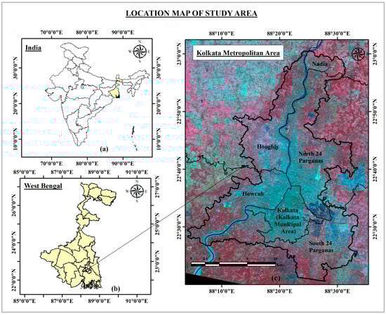
Figure 1.
Location map (a) map of India (b) map of West Bengal (c) Kolkata metropolitan area.
Population growth—The KMA is one of the fastest-growing million-plus cities in India and has witnessed significant migration and overpopulation, burdening existing natural resources [58]. Its population grew from 9.19 million in 1981 to 14.72 million in 2011 and is projected to reach 21.1 million by 2025 [59].
Urban area expansion—The KMA expanded geographically from 361 km2 at the time of independence to 1851.41 km2 between 1991 and 2001 to 1880 km2 at present. Since Kolkata district is the only completely urbanized district in the state, resulting in a stagnant rate of urbanization, the peripheral areas are witnessing rapid urban expansion, characterized by leapfrogging and fragmented built-up area development [15,58].
LULC change—The unrestrained urbanization of KMA has rapidly engulfed agricultural land, naturally vegetated land, and water bodies along the periphery [57]. As per Kolkata and Climate Crisis 2022, shrinkage of waterbodies (including the East Kolkata Wetlands), conversion of agricultural land into built-up areas, loss of agriculture lands in peri-urban areas to construction, damages caused by soil salinization in the aftermath of cyclones, etc., are significant LULC changes in the KMA [60,61].
Pollution—As a progressive metropolitan area, the study area is home to several industries based on steel, heavy engineering, pharmaceuticals, electronics, textiles, food processing, information and technology (IT), and more [57]. Increasing developmental activities and unplanned urban growth have left it to deal with issues like increasing air and land surface temperatures, water and air pollution, poverty, excessive migration, increasing slum population, traffic congestion and various other socio-economic problems.
Diminishing vegetation cover and increasing temperatures—Ray et al. (2023) [59] observed that the urban built-up area has expanded from 20.21% in 1989 to 30.05% in 2019 of the total area of KMA, whereas the area occupied by vegetation and homestead under plantations has decreased from 10.18% and 32.40%, respectively, in 1989, to 9.73% and 19.57%, respectively, in 2019. An expanding urban area with shrinking vegetation cover increases the possibility of the study area experiencing higher LST. The results of studies based on the Kolkata district and its surrounding areas that make up KMA show an increase in LST with the expanding urban built-up area and diminishing vegetation cover that aligns with the findings of [51,62], which are studies conducted on various urban areas around the world [8,63].
Extreme weather events—The study area has been experiencing intense heatwaves in recent times, which have been linked with the ongoing global climate change. Study [64] discusses the erratic nature of rainfall in the study area observed over a number of decades, leading to extreme conditions like urban flooding and droughts.
Cons of the geography and location of the study area—Owing to its proximity to the coast, the study area is more vulnerable to climate change impacts like rapid sea level rise, erratic rainfall, cyclones and storm surges, and coastal flooding. Based on the following issues, KMA was selected for this study.
2.2. Data and Materials Used
Satellite images from Landsat 5—Thematic Mapper (TM) for the years 2000, 2005 and 2010 and Landsat 8—Operational Land Imager (OLI) and Thermal Infrared Sensors (TIRS) for the years 2015 and 2020 were obtained for this study. Owing to the recent increase in LST, UHI phenomenon and heatwaves in the area, most studies pertaining to this area have focused on the post-2000s. The aim was to collect images from the pre-summer months in India, which would be cloud-free and free from the bias caused by the summer heat in the processed data. Despite trying to maintain parity in the images, a cloud-free image for processing was not available for January 2015. Therefore, the next best alternative of March 2015 was considered.
ArcGIS Version 10.8 software was used for the computation of ECI, hotspot and consistency analysis and obtaining data for correlation analysis. The MOLUSCE plugin, QGIS Version 2.8.3, was used for future prediction. Two shapefiles were used for the study area: one for the Kolkata district and the other one for the KMA.
2.3. Methodology
2.3.1. Image Pre-Processing
Landsat 5 and 8 data (Table 1) were procured from USGS. All satellite data were pre-processed with Chavez’s COST model for atmospheric corrections [65]. Image bands (Table 2 and Table 3) were stacked, and standard False Colour Composites (FCC) were generated using the Near Infrared (NIR), red and green bands for Landsat 5 and 8 images (Figure 1b).

Table 1.
Product details of Landsat 5 and 8.
Table 2.
Band details and resolutions of Landsat 8–OLI and TIRS, used in this study [66].
Table 3.
Band details and resolutions of Landsat 5—TM, used in this study [67,68].
2.3.2. Image Processing
- (1)
- Computation of Spectral Indices
Spectral indices offer a semi-automated method of identification and extraction of desired LULC features [69]. These indices were devised based on the spectral reflectance characteristics of earth surface features and provide more information than raw image bands [70]. When compared with conventional techniques, identification of specific earth surface features using spectral indices has proved to be more accurate, and efficient, has simple calculations that might not always require image pre-processing, and uses multiple band combinations and ratios that involve strong reflectance from the target feature while offering adequate distinction between other LULC features [71,72]. Spectral index-based identification and extraction of desired LULC features were incorporated in this study.
- (a)
- NDVI—Depending upon the spectral characteristics of vegetation, NDVI, a dimensionless index, which describes the difference between visible and near-infrared reflectance of vegetation cover, can be used to estimate the density of green on an area of land [73].The value of NDVI ranges from −1 to 1, where a score of 0 or close to 0 indicates non-vegetated lands, a negative score of −1 or close to −1 indicates water, snow, etc., and a positive score nearing +1 indicates greater chlorophyll content, vegetation health and vigour, greater vegetation density, etc. [74].The NDVI thus produced for the entire image was used for two purposes: (a) the entire image was stretched for ECI estimation and (b) the study area shapefile was used to extract the study area from the original NDVI image for the purpose of creating maps and correlation analysis. The entire process was applied to images of all 5 years.
- (b)
- Modified Normalized Difference Water Index (MNDWI)—It utilizes green and SWIR or MIR bands to identify water bodies and is proven to be the best fit for extracting water bodies in a built-up area, as it successfully suppresses the noise generated by non-water features like built-up areas, vegetation and soil [75]. Thus, the water bodies of KMA were identified using the following formula for MNDWI:The water bodies were identified using the MNDWI for the entire image. KMA was extracted from the MNDWI image using the study area shapefile. The image was reclassified into non-water and water using appropriate thresholds. It was then segmented, and separate rasters were created for non-water and water, which were then converted to shapefiles of non-water and water. This process was applied to images of all 5 years.
- (c)
- Modified Bare Soil Index (MBI)—The spectral similarity of built-up areas and bare lands often lead to an unrealistic representation of urban spaces [76]. Bare soils, e.g., agricultural fallow, can change due to soil moisture, vegetation cover, cropping patterns, and seasons, whereas built-up areas do not exhibit such transformations, as they lack the soil–plant–water interaction [77]. Thus, it was used to identify the bare land areas using appropriate thresholds in this study, using the following equation:KMA was extracted from the MNDWI image using the study area shapefile. The image was reclassified into non-bare and bare using appropriate thresholds, selected after verification from Google Earth Pro and field inputs. It was then segmented, and separate rasters were created for non-bare and bare, which were then converted to shapefiles of non-bare and bare. This process was applied to images of all 5 years.
- (d)
- Built-Up Area Demarcation—Impervious Built-up Index (optical), IBUIopt (Equation (4)) was adopted for this study owing to its ability to use the spectral reflectance characteristics of built-up areas eliminating noise from vegetation and water [78,79,80].where,The study area was extracted using the metropolitan area shapefile and the bare soil areas were eliminated using the MBI shapefile forming the product BUINB (Built-up Index Non Bare). In order to bring the index values for built-up areas within a common range of 0–1, the product was normalized, forming Normalized BUI Non Bare (NBUINB):The product was then reclassified into a binary image of built-up areas and non-built-up areas using the appropriate threshold, based on FCC images, Google Earth Pro and field inputs, for the creation of a built-up area map. Values close to 1 indicated built-up areas and those close to 0 indicated non-built-up areas. An accuracy assessment was performed to obtain the accuracy level and kappa coefficient of the method used for built-up area demarcation. Using Google Earth Pro and field verification, the classified and ground truth values to points were validated and a confusion matrix was generated. It was applied to images of all 5 years.
- (2)
- Computation of thermal-based Environmental Criticality
- (a)
- LST Estimation—The thermal infrared remote sensing technique has been applied in multiple studies based on the urban climate and environment, mainly for the retrieval of LST, an important parameter in the study of urban thermal environment and dynamics, and analysis of its spatio-temporal variation and relationship with surface features, e.g., vegetation, water bodies, and built-up area. A series of airborne and space-borne sensors, like AVHRR, MODIS, Landsat TM/ETM+, ASTER, TIMS, HCMM and AVHRR, was devised for collecting thermal data [25,81]. Standard steps were adopted for calculating LST from Landsat data.
- i
- Calculation of Radiance of Band 10 for Landsat 8 and Band 6 for Landsat 5—where Lλ—Top of the Atmosphere (TOA) spectral radianceML—Radiance Multiplicative BandAL—Radiance Additive BandDN—Quantized and calibrated standard product pixel values.
- ii
- Calculation of Satellite Brightness Temperature from Bands 10 and 6 for Landsat 8 and 5—where K1 and K2 are band-specific thermal conversion constants obtained from Metadata. K1 = 607.76 for Landsat 5 and 774.8853 for Landsat 8. K2 = 1260.56 for Landsat 5 and 1321.0789 for Landsat 8. This step was performed to obtain the final results in Celsius from Kelvin. It is executed by adding absolute zero which is approximately equal to −273.15.
- iii
- Calculation of NDVI—In Landsat 8, band 5 and band 4 represent NIR and red, respectively. In Landsat 5, band 4 and band 3 represent NIR and red, respectively. The bands were entered in the raster calculator accordingly.
- iv
- Calculation of Proportional Vegetation (Pv)—where NDVImax—Maximum value of NDVI, NDVImin—Minimum value of NDVI.Pv = [(NDVI − NDVImin)(NDVImax − NDVImin)]2
- v
- Calculation of Land Surface Emissivity (LSE)—LSE = 0.004 ∗ Pv + 0.986
- vi
- Calculation of LST—where BT—Brightness Temperature of Thermal Bandsw—Wavelength of emitted radianceP = (h*c)/s = 1.438 ∗ 10−2 mkwhere h—Planck’s constant (6.626 ∗ 10−34 Js)c—Boltzman constant (1.38 ∗ 10−23 J/K)s—Velocity of light (2.998 ∗ 108 m/s)The LST thus produced for the entire image was used for two purposes: (a) the entire image was stretched for ECI estimation and (b) the study area shapefile was used to extract the study area from a non-stretched LST image for the purpose of creating the map.The entire process was applied to images of all 5 years.
- (b)
- ECI Estimation—To estimate the ECI for the entire image for each year, the stretched images of LST were divided by the stretched image of NDVI, as stretching enhances the contrast for processing LST and NDVI data and prevents errors, such as infinite ECI values, that could result from 0 values in the stretched NDVI dataset [14,16].The study area shapefile was used to extract the study area from ECI images. Using the non-water shapefile created in Section 2.3.2 (1b), the non-water areas were extracted from the ECI images of the study area. Thus, water bodies were eliminated from the ECI images of the study area, as per [16]. This process was applied to images of all 5 years.
- (3)
- Consistency and Hotspot Analyses of ECI
- (a)
- Spatio Temporal Thermal–based Environmental Criticality Consistency Index (STTECCI)—The Spatio Temporal Thermal Consistency Index (STTCI) is a novel technique proposed in [15], developed to highlight the surfaces that consistently record high LST in the user-defined temporal span for the study area, KMA, which was later delivered successfully with an accuracy level close to 90% and the kappa coefficient exceeding 0.85. This idea was incorporated in this study as STTECCI to highlight the areas that have consistently recorded higher levels of environmental criticality over the period considered for this study, as these areas should be the ones to be prioritized at the time of devising mitigation measures and policies. Thus, in our study, this analysis was based on the ECI (Section 2.3.2 (2b)).The STTECCI was conducted in two steps:
- i
- The Spatial Consistency Index (SCI) was calculated using:
- ii
- The mean of the output products offered a long-term picture of ECI in the study area and highlighted those areas that have consistently recorded high and low ECI.
- (b)
- Getis-Ord Gi* technique of hotspot analysis—The Getis-Ord Gi* technique of hotspot analysis, a local statistical method, was devised to identify the statistically significant spatial clusters of high and low values of a phenomenon or feature within a limited geographical area [24]. A cluster of high values is considered to be a hotspot, while a cluster of low values indicates a cold spot.Hotspot analysis was conducted on LST to locate the LST hotspots and understand the impact of LULC change and urbanization on UHI and highlight the critical areas that require immediate attention and actions to resolve the issue. In this study, the STTECCI raster (Section 2.3.2 (3a)) was used for hotspot analysis, with 5000 randomly generated points with ECI values as input, fixed distance band as conceptualization of spatial relationships and Euclidean distance as distance method used to obtain high and low ECI value clusters. The high/low clustering report was also produced using the Getis-Ord general G technique.
- (4)
- Correlation Analysis
Correlation analysis is used to study the association or relationship between two (or more) quantitative variables [82]. The index rasters (NDVI, NBUINB, MBI) were combined temporally using ‘Cell Statistics’ where mean (average) was used as overlay statistics. Point shapefiles for agriculture, plantation, open fields, natural vegetation, urban and rural build-up, industrial, agricultural fallow and lightly vegetated open ground were made. With the help of Basemap imagery, FCCs, Google Earth and visual image interpretation elements, points for the aforementioned features were marked. Values to these points in the point shapefiles were extracted from the combined rasters of their respective land cover and use (Section 2.3.2 (1)) and STTECCI raster (Section 2.3.2 (3a)). The attribute tables for the point shapefiles were then converted to Excel sheets, scatter plots were constructed, and the correlation coefficient (r) and coefficient of determination (r2) were computed.
2.3.3. Predictive Modelling
ECI for the years 2030 and 2040 were predicted using the MOLUSCE plugin in QGIS Version 2, which is based on the combination of two models, CA and ANN [46,83,84] and uses the strength of both. The CA method models the state of the phenomenon based on the previous state of the cells within a neighbourhood according to a set of transition rules [85]. ANN is similar to the structure of synaptic connections for distributed and parallel information processing of the brain, and possesses the ability to self-learn and self-adapt [86]. The pros of using ANN are (a) it is best suited for cases where the underlying processes and relationships are hard to understand or unknown and display chaotic properties, unlike the Markov Chain, which works better when the trends within the phenomenon are known, and (b) it can model complex nonlinear relationships, which is advantageous for the prediction and simulation of LULC and LST [85,86]. CA can effectively comprehend land-use systems and their underlying dynamics, particularly when combined with ANN. Since CA-ANN is based on “what-if” scenarios, it can be used in land change simulation studies.
MOLUSCE was employed in this study, owing to it being an open-source platform used in various studies for predicting LST, one of two decisive parameters that are directly related to ECI [87,88]. These studies predicted an increase in area under high LST categories with expanding built-up area and decreasing vegetation cover. Since the future prediction of ECI is a novel attempt, the execution of it was heavily based on existing literature and personal cognition.
The MOLUSCE plugin consists of seven elements and the following steps show how they were used:
- (a)
- Inputs: For 2030, years 2010 and 2020 were used as initial and final years, respectively and for 2040, years 2000 and 2020 were used as initial and final years, respectively. The initial and final ECI rasters were reclassified and converted to discrete data. NDVI, LST and NBUINB were used as spatial variables, and, following this, such variables on which LST is dependent were used as input parameters for the simulation.
- (b)
- Evaluation Correlation: Pearson’s correlation, Crammer’s coefficient, and joint information uncertainty are inbuilt correlation methods in the MOLUSCE plugin. Pearson’s correlation was used to evaluate the correlation between the spatial variable factors used for this study.
- (c)
- Area Changes: It produces a transition probability matrix and a change map showing the fraction of pixels that have transitioned from one class to the other. The proportion of area changes in sq. km in each category of ECI was computed in this step.
- (d)
- Transition Potential Modelling: The Artificial Neural Network—Multi-layer Perceptron (ANN-MLP) method was selected for transition potential modelling. Based on available literature [89] and multiple permutations and combinations, Neighbourhood was set at 1 px, learning rate at 0.001, maximum iterations at 1000, hidden layers at 10 and momentum at 0.001. This approach utilized geographic factors and information about changes in ECI for calibration and modelling [90].
- (e)
- Cellular Automata Simulation: The number of iterations was set as 1 and simulated maps for 2030 and 2040 were produced based on their respective initial and final years and associated information using cellular automata simulation.
- (f)
- Validation: In order to validate the accuracy of the simulated map, MOLUSCE uses Kappa statistics that include % of correctness, standard Kappa, Kappa histogram, and Kappa location [91]. Following [92], simulated ECI maps of 2030 and 2040 were validated using the actual ECI map of 2020.
The flow diagram of the approach is summarized and depicted in Figure 2.
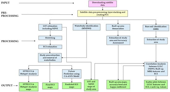
Figure 2.
Flow diagram of the approach.
3. Results
3.1. Thermal-Based ECI
- (1)
- NDVI—Figure 3 reflects on the status of vegetation cover in the study area. A considerable portion of the peripheral areas of the KMA, comprising Howrah in the southwest and west, Hooghly in the west, northwest and north, Nadia in the north and northeast, North 24 Parganas in the north, northeast and east and South 24 Parganas in the southeast and south (Figure 1a), had dense vegetation until 2010, following which a decline in vegetation can be witnessed in 2015 and 2020.
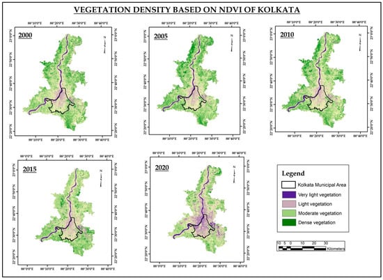 Figure 3. NDVI maps of the study area.Section 2.1 discusses the linear development of the metropolitan’s built-up area along the Hooghly River, owing to it being a major source of water for all sorts of activities, thus attracting settlements and industries. Thus, the consistent classification of the Hooghly River banks under low vegetation, from ‘Light’ until 2010 to ‘Very Light’ in 2015 and 2020, can be attributed to the spread of the built-up area, which also consists of Kolkata district and Howrah. The built-up areas were classified under ‘Moderate’ until 2010, and from ‘Light’ in 2015 to ‘Very Light’ vegetation in 2020. It was previously mentioned in Section 2.1 that Kolkata district is the only completely urbanized district in the state. This information supports the change observed in the vegetation cover, from ‘Light’ to ‘Very Light’ until 2010, where the absence of vegetation was restricted in the northwestern part along the river bank, to the entire district being categorized under low vegetation in 2015 and 2020. In the neighbouring districts, the transformation of vegetated lands into built-up areas can also be observed.A decrease in vegetation cover was also observed in the East Kolkata Wetlands (EKW). EKW, located on the eastern fringe of Kolkata district, was recognized as a Wetland of International Importance by the Government of India, in accordance with Criteria 1 of the Ramsar Convention in 2002 [93]. It offers a cost-efficient Nature-Based Solution (NBS) for sewage treatment of the district, utilizing nutrients from wastewater to produce fish, vegetables, and paddy, trapping carbon and reducing greenhouse gas emissions and acting as a flood buffer on the peri-urban interface. Wetlands also have a cooling effect on surrounding areas, and the air and land surface temperatures are reduced by vegetation via evapotranspiration and canopy shading (Section 1) and water via evaporative cooling [10,94], potentially reducing environmental criticality and UHI effect. However, rapid urbanization and land conversion induced by the encroachment of built-up areas have disturbed the equilibrium of the wetland ecosystem, hampering the quality of ecosystem services that they provide and disrupting the lives and livelihood of their residents, which is not just the case for EKW but for wetlands across other Asian countries like Bangladesh, Nepal, Sri Lanka [95].
 - (2)
- LST—Shrinking vegetation cover plays a key role in the rising LST (Section 1). Figure 4 shows that the LST is high, particularly in those areas that lack vegetation (Figure 3), where the maximum LST ranges between 28 °C to 39 °C approximately.
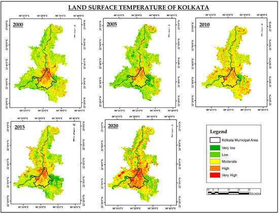 Figure 4. LST maps of study area.The central part of the agglomeration, which is occupied by Kolkata district and part of Howrah, has consistently recorded ‘Moderate’ to ‘Very High’ LST. The northwestern (NW) part of Kolkata and the eastern part of Howrah, on opposite banks of Hooghly River, were classified under ‘High’ to ‘Very High’ LST from 2000–2020, owing to the absence of vegetation, indicating the presence of built-up areas. The rest of the area was classified under ‘Low’ to ‘Moderate’ LST until 2005. Since 2010, these areas have also witnessed a rise in LST, which could indicate the clearing up of vegetated lands to make space for built-up areas. LST has also increased along the right and left banks of the river with progress in developmental activities over the years.Figure 4 also shows that major portions of the neighbouring districts of the Kolkata district or the peripheral areas that are occupied by rural settlements [96] and that are under vegetation cover have lower LST. Rural areas have naturally vegetated surfaces [27] and are surrounded by agricultural plots, which could be one of the factors that could help in the identification of rural areas. Thus, the amount of energy stored is lower compared to the urban artificial surfaces; hence, the LST is lower in comparison to the urban surfaces. As development progressed and the urban areas started encroaching upon the surrounding areas with vegetated land, the LST started showing an upward trend from 2010. Since these areas have a certain degree of vegetation cover, not as dense as there were previously, these areas now have low to moderate LST. The central part, which has witnessed maximum growth, has the highest LST. With the gradual increase in built-up area by clearing vegetation cover, the LST can be seen to have increased gradually from the central part to the peripherals of the agglomeration. The water bodies of EKW were classified under ‘Very low’ to ‘Low’ LST, whereas the land areas have witnessed a rise in LST, which could be an outcome of clearing up vegetation cover for developmental activities.
 - (3)
- ECI—It can be inferred from Figure 5 that environmental criticality follows a trend similar to LST. Areas with very low vegetation cover have the highest LST and consequently the highest criticality rate. The mean of the image statistics (Table 4) clearly indicates the rising criticality over the years. The NW part of Kolkata Municipal Area and the eastern part of Howrah were consistently classified under ‘Very High’ criticality over two decades. The rest of the Kolkata Municipal Area has seen a gradual rise in ECI, from ‘Very Low’ to ‘Moderate’ in 2000 and 2005, from ‘Moderate’ to ‘High’ in 2005 and 2010 and ‘High’ to ‘Very High’ in 2015 and 2020. The peripheral areas have witnessed a significant rise in ECI over the years, and they were classified under ‘Very Low’ to ‘Low’ until 2010 with some pockets having ‘Moderate’ to ‘High’ ECI. In 2015 and 2020, spatial decreases in the areas under ‘Very Low’ and ‘Low’ and increases in areas under ‘Moderate’ to ‘High’ were observed. Even then ‘Very Low’ to ‘Low’ ECI regions are restricted to the outer reaches of the peripheries. ECI has increased along the banks of the river over the years as well.
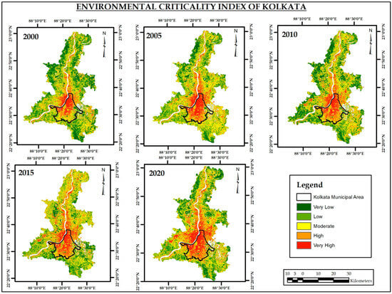 Figure 5. ECI maps of study area.
Table 4. Image statistics of ECI of study area, without water bodies.After eliminating the water bodies from the EKW region, it can be observed that in 2000, this region had low criticality rates. It was classified under ‘Moderate’, with some pockets having ‘High’ criticality in 2005 and 2010. In 2015 and 2020, a major portion was facing ‘High’ to ‘Very High’ criticality, with some pockets having ‘Moderate’ to ‘Low’ criticality.Spatial increases in the areas under ‘High’ to ‘Very High’ and decreases in the areas under ‘Very low’ to ‘Low’ were observed over a span of 20 years. The rise in environmental criticality over the years can be attributed to the progress in developmental activities, construction and expansion of residential, commercial, industrial complexes, etc.
Figure 5. ECI maps of study area.
Table 4. Image statistics of ECI of study area, without water bodies.After eliminating the water bodies from the EKW region, it can be observed that in 2000, this region had low criticality rates. It was classified under ‘Moderate’, with some pockets having ‘High’ criticality in 2005 and 2010. In 2015 and 2020, a major portion was facing ‘High’ to ‘Very High’ criticality, with some pockets having ‘Moderate’ to ‘Low’ criticality.Spatial increases in the areas under ‘High’ to ‘Very High’ and decreases in the areas under ‘Very low’ to ‘Low’ were observed over a span of 20 years. The rise in environmental criticality over the years can be attributed to the progress in developmental activities, construction and expansion of residential, commercial, industrial complexes, etc.
Thus, it can be seen that the results of this study align with the findings of global studies like [54] based in Chicago (USA), ref. [4] based on Milan, Bologna, Florence and Rome (Italy), ref. [62] based on the National Capital Region (Ottawa-Gatineau) and the Greater Toronto Area, ref. [23] based on Bangkok Metropolitan Area, Thailand, which highlights the fact that rising urbanization and the consequent decline in vegetation cover, increase in built-up area, rising LST and formation of heat islands are a matter of utmost concern in almost all urban areas across the world. Studies based on our study area, e.g., [56,97] and other tropical cities in the Indian subcontinent.
3.2. Consistency and Hotspot Analyses of ECI
- (1)
- STTECCI—For the purpose of mitigation measures and policies, the ‘High’ to ‘Very High’ ECI zones were mainly focused upon in this study. Since averages and standard deviations were involved in the computation of STTECCI, the original ECI values were modified further, giving a range of −4.59 to 5.90 for the study area. Furthermore, 0.46–5.90 is the range for high to very high ECI, which was recorded in the urban built-up areas and industrial zones.With the help of Figure 6, the Kolkata Municipal Area was identified as the most significant zone of consistently ‘High’ to ‘Very High’ ECI, owing to its completely urbanized nature, the highest concentration of built-up area and the highest population density in metropolitan Kolkata. The eastern part of Howrah, along the bank of the Hooghly River, is another urbanized area with the same level of criticality as the Kolkata Municipal Area. Hooghly River, being the major source of water in the study area, has attracted settlements and industries that include power plants like the Bandel Thermal Power Station and jute mills to develop along its banks. Industrial zones, like the ones located in Howrah, also fall under the ‘Very High’ ECI category. Besides urban areas, industrial zones also generate a considerable amount of pollutants and wastes that are responsible for the deteriorating air and water qualities. As one moves away from the core urban and industrial centres, the criticality decreases. These zones have moderate environmental criticality. The areas located in the absolute peripheries have rural built-up areas [96] dominated by natural vegetation and agriculture, which could be the reason behind having ‘Low’ to ‘Very Low’ criticality.
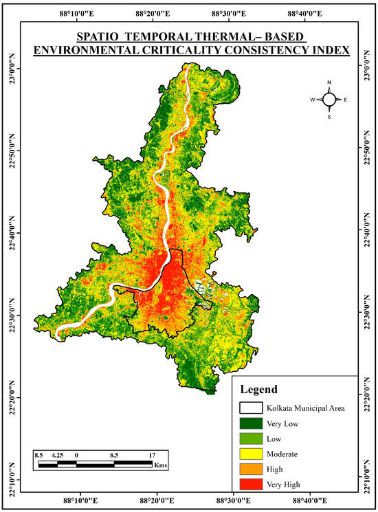 Figure 6. STTECCI.
 - (2)
- Hotspot Analysis—A significant ECI hotspot can be located in the center of KMA (Figure 7b), which is the core urban area in the agglomeration. This cluster has a Gi*z-score greater than 2.58 and a Gi*p-value as low as 0.00–0.01 (Table 5). Thus, it can be said that it shows a statistically significant spatial cluster of high ECI values. With a 99% confidence level, it can be stated that the possibility of this high-value cluster being a result of random chance is less than 1%. The same can be inferred from the High–Low clustering report in Figure 7a as well, where the z-score is 10.59 (~) and the p-value is 0.
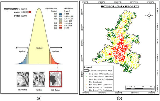 Figure 7. (a) High–low clustering. (b). Hotspot analysis of ECI.
Table 5. Gi*z-scores, p-values, Gi Bin and Gi*Hotspot classes.
Figure 7. (a) High–low clustering. (b). Hotspot analysis of ECI.
Table 5. Gi*z-scores, p-values, Gi Bin and Gi*Hotspot classes.
The policy-making process can gain from the mapping and identification of environmentally critical areas in KMA, using STTECI and hotspot analysis, in a number of ways. Policymakers can use these maps in various ways: (a) to visualize the ground reality and make decisions based on data and facts; (b) to focus development and management plans, mitigation strategies, and resource allocation on areas that need immediate attention; (c) to communicate with the masses and raise public awareness regarding environmental challenges; (d) by identifying zones prone to extreme thermal events, they can prepare plans to reduce damage to lives and infrastructure; and (e) in the face of global climate change, these studies increase the flexibility of the policy-making process by enabling them to modify strategies in response to evolving data from long-term environmental monitoring and assessment.
3.3. Mapping of Built-Up Area
Figure 8 presents a clear picture of the expansion of the built-up area from the central part of metropolitan Kolkata, occupied by parts of two districts, Kolkata and Howrah, to the peripheral areas that include Rajarhat, Barrackpore, Barasat, Madhyamgram, etc., in the east, and Maheshtala, Sonarpur-Rajpur, etc., in the southeast, south and southwest.
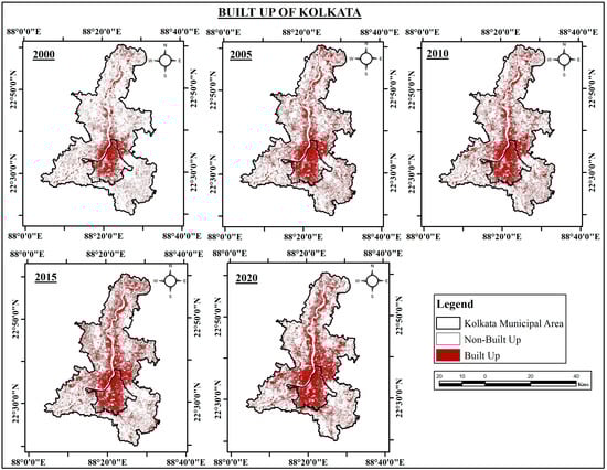
Figure 8.
Built-up maps of the study area.
The northwestern part of Kolkata district and eastern part of Howrah, located in the vicinity of Hooghly River, has had the highest concentration of built-up areas since 2000. As per the images, from 2005–2020, a significant increase in the area and compactness of built-up areas from the northwestern to the other parts of the Kolkata district, barring the eastern part occupied by the EKW, can be observed. It could be expressed that, owing to the presence of the wetlands, even though the built-up areas have increased, they are comparatively lower than the rest of the region.
By virtue of being the major source of water in the region, the Hooghly River has attracted settlements and industries to develop along its banks. The built-up area has also increased in the interiors of other districts in the metropolitan area as well, but the major development has occurred in Howrah, North and South 24 Parganas, besides Kolkata district.
3.4. Correlation Between LULC Features and ECI
- (1)
- Agriculture, Plantations and Open Fields—Figure 9a and Table 6 show a negative or inverse correlation between agriculture, plantations and open fields and ECI. For positive NDVI values that indicate the presence of some kind of vegetation, ranging between 0.05 and 0.45 approximately, the ECI values range between −2 and 0.75 approximately. This indicates that areas with crops and plantations and open fields have low environmental criticality.
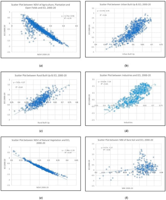 Figure 9. (a,b) show a correlation between agriculture and ECI, (b–d) show a correlation between built-up areas and ECI, (e) shows a correlation between natural vegetation and ECI and (f) shows a correlation between bare soil and ECI.
Table 6. Showing ‘r’, ‘r2’ and spatio-temporal ECI values for LULC features, 2000–2020.
Figure 9. (a,b) show a correlation between agriculture and ECI, (b–d) show a correlation between built-up areas and ECI, (e) shows a correlation between natural vegetation and ECI and (f) shows a correlation between bare soil and ECI.
Table 6. Showing ‘r’, ‘r2’ and spatio-temporal ECI values for LULC features, 2000–2020. - (2)
- Built-up—LST and vegetation are two important parameters used for the computation of ECI. Thus, it could be assumed that if the expansion of the built-up area is the cause of the depletion of vegetation cover and elevated temperature levels (Section 1), it would also have an impact on the ECI of the study area. It could be inferred from Figure 5 and Figure 8 that both the built-up area and areas categorized under high environmental criticality have increased, and the high criticality zones coincide with the densely built-up areas of KMA.The urban built-up areas have a positive correlation with rising ECI (Figure 9b and Table 6). It can be observed from the graph that a cluster of points has formed with an index value of built-up areas ranging between 0.525–0.675, approximately, for which the ECI values range between 0 and 3. Rural built-up areas, by virtue of being part of built-up areas, are positively correlated with the ECI (Figure 9c and Table 6), and the index value range is 0.45–0.625, approximately, for which the ECI ranges between −1.5 and 1.5, approximately, which is comparatively lower than urban areas. Figure 6 also shows that the urban areas have consistently recorded ‘High’ to ‘Very High’ criticality, while the rural areas have consistently been classified under ‘Very Low’ to ‘Moderate’ criticality. The industrial areas are positively correlated with rising ECI (Figure 9d and Table 6). Industries, again, by virtue of being a form of build-up and being constructed using materials similar to that used in urban built-up features, have similar optical and thermal properties, which may explain the occurrence of a cluster in the graph, ranging between 0.5–0.7, approximately, on the x-axis. For industrial zones, the ECI ranges between −1.2 and 3, approximately, which is almost similar to that of urban build-up.
- (3)
- Natural Vegetation—The peripheries were classified under ‘Very Low’ to ‘Moderate’ LST over the years (Figure 4). Therefore, natural vegetation, with the capability to absorb greenhouse gases, modulates surrounding air temperature and lowers the criticality levels. Figure 5 and Figure 6 show that the peripheries of KMA were consistently classified under high vegetation, low LST and low ECI levels. NDVI undoubtedly has a strong inverse correlation with ECI, which indicates that environmental criticality is lower and under control in those areas that are dominated by vegetation cover. The values of NDVI for natural vegetation range between 0.12–0.40, for which the ECI ranges between –2 and 0.5. A cluster forming on the x-axis, along the trend line between 0.15–0.35, for which the ECI ranges between −1.60 and 0 approximately, can also be seen in the image.
- (4)
- Bare lands—In this study, appropriate satellite imageries from the pre-summer season for the years 2000, 2005, 2010, 2015 and 2020, avoiding the cloud cover, were collected. Certain bare areas in the southeastern part of KMA, in the vicinity of EKW were identified as agricultural fallow with the help of Basemap imagery, for recent years, and Google Earth Pro, for previous years, while others appeared to be open grounds partly covered with very light vegetation like grasses (Figure 10n,o).
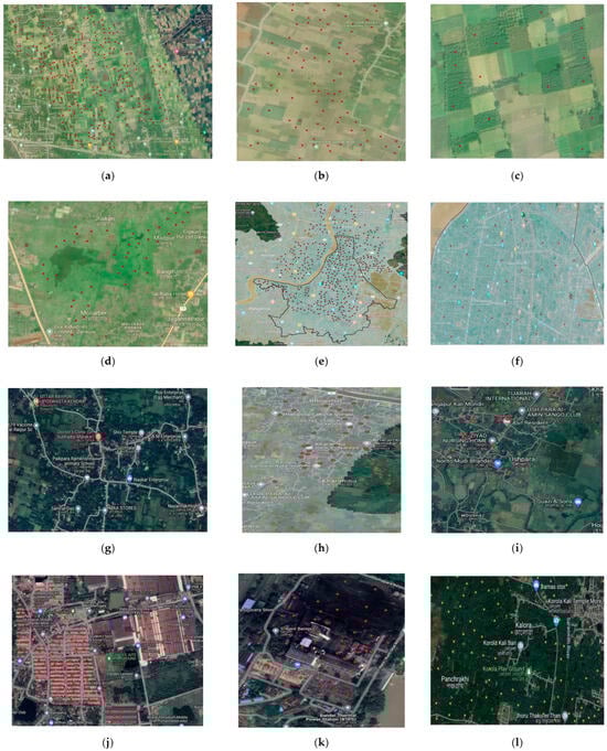
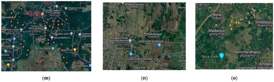 Figure 10. (a,b) show agricultural plots, (c) depicts plantations, (d) shows open fields, (e,f) show urban built-up areas, (g–i) depict rural built-up areas, (j,k) show industrial areas, (l,m) show naturally vegetated lands, (n,o) show bare lands in KMA.For the cluster forming between 0.32 and 0.36 approximately, the ECI values range between −0.5 and 1, approximately. The highest value of the range for ECI can be classified under moderate to high criticality, but this could be attributed to LST values that are supposed to be lower in the pre-summer than in the peak summer and form the numerator while ratioing. The weak correlation could indicate that the effect of bare soils on the criticality of an area is insignificant. The LST of such lands vary with their moisture content. When under crop cover, the irrigation processes that take place indicate that the soil, underneath crops, is moist. This results in higher vegetation (NDVI), lower LST and lower criticality. Thus, moist bare lands produce lower LST than the drier ones.
3.5. Future Prediction of ECI
The studies indicated the use of the CA-ANN technique on ECI [87,88]. These studies have applied the CA-ANN technique for predicting the LST of their respective study areas, a decisive parameter of ECI, and directly related to it, and have observed an increase in it over time. The thermal-based environmental criticality of Kolkata appears to be increasing following the trend of increases in LST with the decline in vegetation cover and expansion of the built-up area. Figure 11 gives a visual representation of the spatial pattern of changing ECI. It shows that in the upcoming decades, the percentage of land area under high ECI categories is expected to increase. This increase was observed to take place in areas that are today occupied by urban built-up areas and industries (Figure 8). The LST (Figure 4) and ECI (Figure 5) images indicate that the urban areas are zones of high LST and ECI; Figure 9b, d confirms the same. Figure 6 highlighted the urban and industrial areas as zones that have consistently recorded high LST over the period considered for the study and Figure 7b identifies this zone as a significant ECI hotspot.
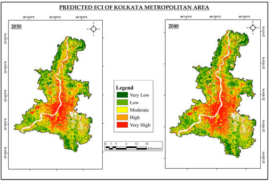
Figure 11.
Predicted ECI of study area.
Table 7 shows the validation Kappa statistics revealing the accuracy in the prediction which is more than 90% for both 2030 and 2040 and Table 8 offers a summary of the area change data generated by the MOLUSCE plugin. It indicates a significant decline in the percentage of land area under low ECI categories, from 50.02% in 2000 to 35.6% in 2040. It can also be inferred from the table that the land area under the high ECI categories is predicted to increase significantly from 23.93% in 2000 to 36.56% in 2040. However, the percentage of areas under moderate ECI is expected to witness a gradual increase from 26.05% in 2000 to 27.84% in 2040.
Table 7.
Showing validation Kappa statistics.
Table 8.
Percentage of area in each ECI class.
4. Discussion
Section 3 demonstrates why studying thermal-based ECI is essential for a dynamic metropolitan area like KMA. Rapid urbanization and declining vegetation have led to rising LST and ECI, particularly in urban and industrial built-up areas, which have consistently recorded higher criticality than rural and peripheral regions. These urban areas have become criticality hotspots, and their encroachment into rural lands has begun to affect the latter as well, as discussed in Section 3. To address the current situation and balance economic growth with environmental sustainability in the future, certain mitigation measures must be implemented.
4.1. Mitigation Measures
In order to reduce the rising temperatures (LST and air) and mitigate the UHI effect, thereby reducing the environmental criticality of any region, studies like [16,29,98] have suggested certain strategies. Some of these strategies are already in use in most countries, including India, like:
- (a)
- Planning urban area construction and developmental activities in a way that makes room for free flow of air in urban areas, i.e., reducing the height of structures promotes and ensures the use of appropriate light materials with higher albedos for buildings, pavements, etc., and use of cool pavements [99], landscaping using vertical green spaces in multi-storied buildings and horizontal green spaces on rooftops, incorporation of water bodies, etc.
- (b)
- Incorporation of green infrastructure like green belts around industries in India. As per the guidelines of the Ministry of Environment, Forests and Climate Change, Government of India, a greenbelt should be created along the boundary of industrial complexes with tall, evergreen trees and the total green area including landscaping area should be about 33% of the industry’s area. Greenbelts have now been introduced in urban areas as well. They act as a sink for harmful greenhouse gases generated by vehicles and industries functioning in urban areas and curb the generation of waste heat, thereby reducing temperatures. Certain specific species were suggested by the government based on their ability to manage environmental issues, e.g., Australian Wattle, Neem, Banyan trees, Coconut trees, and Ashoka trees.
- (c)
- The West Bengal Government’s Green City Mission includes the Greening and Blueing plan under its list of schemes. The Greening plan is concerned with urban afforestation, creation and revival of parks, nurseries, floriculture, pocket forests, and plantations along the median of the roads while the Blueing plan is associated with the conservation of water bodies, water-based recreation, canal/waterfront development and hedges along the waterfront.
- (d)
- Conservation of wetland ecosystems is also deemed to be important in managing environmental criticality. Thus, plans like the East Kolkata Wetlands Management Action Plans for preserving EKW were put into effect.
4.2. Contributions and Limitations
This study was able to make the following contributions as per the objectives set for it in Section 1:
- (1)
- This study made a novel attempt to identify and map those areas in a dynamic UA like KMA, that were experiencing severe heat-related environmental issues owing to the rapid population growth, urbanization and urbanization-induced land cover transformations. The quantification of environmental criticality contributed towards a deeper understanding of the impacts of rapid and unrestrained urbanization on the local climate and ecosystem. These changes have intensified heatwaves in recent times and have disrupted the weather pattern leading to frequent occurrence of extreme events like droughts and floods. The EKW have also been driven into a critical state owing to the rising encroachment by urban areas, thereby hampering the ecosystem services offered by it and disrupting the lives and livelihood of its residents (Section 3.1(1)).
- (2)
- With consistency and hotspot analysis, this study was able to further explore this relatively new concept of ECI in-depth and provide new insights. An in-depth understanding of the consistency of the level of criticality in the urban and industrial areas would help policymakers in making data-driven informed decisions. By focusing the mitigation strategies and resources on such areas, they could help bring down the level of environmental criticality. The application of geospatial techniques for monitoring and assessment could increase the flexibility of the policymaking process in the face of global climate change.
- (3)
- By quantifying the relationship between LULC features and ECI, this study can assist policymakers in striking a balance between economic growth and development and conservation of the environment. Some of the policies were discussed in Section 4.1. This step also proved the hypotheses, on which the entire study was based, true.
- (4)
- Forecasting the future can aid in the creation of appropriate strategies for future economic growth and development that will not jeopardize the health of the environment.
However, this study is also not without limitations: (a) since the study involved multiple elements associated with ECI, the quantification and validation of other parameters are not discussed in detail; (b) ECI could be calculated using LST and a built-up index, but our study area faced noise from bare lands and NBUINB (Section 2.3.2 (1d)), the product for which is a binary image and could not be used for image multiplication, which was determined to be our most suited method for our study; (c) predictive models like CA-ANN are based on parameters entered into the system, but the outcomes vary with ground reality, as they can be influenced by policy changes, climate variations, extreme events or economic development; and (d) socio-economic trends and patterns were not within the scope; mainly thermal based assessments were performed. Despite its limitations, this study can be recreated to check its accuracy over other study areas, new insights can be provided and there is scope for further improvements.
5. Conclusions
Thus, it can be concluded that different LULC features have different impacts on ECI. While natural vegetation lands and agricultural plots with crops or some sort of vegetation have a negative correlation with ECI, owing to the evapotranspiration and canopy shading by trees that reduce land surface and air temperatures, respectively, built-up areas, mainly urban and industrial, are positively correlated. Built-up areas are constructed with low albedo materials with high heat absorbing capacity, and witness a dearth of vegetation cover due to land conversion and experience the urban canyon effect that restricts the free flow of air and generates waste heat in abundance, thereby increasing temperatures and imposing heat island effect, which is quantified and reflected as high ECI in these areas. All the figures and charts in this study prove the fact that rising environmental criticality is indeed an outcome of LULC change from naturally vegetated lands, agricultural plots, bare lands, and rural settlements to urban residential and industrial areas. This has become a grim reality for most metropolitan areas around the world, especially the rapidly developing South Asian countries, of which KMA is a significant part. KMA’s urban areas have already started bearing the brunt of urbanization, which have induced climate change in the forms of severe heat waves, floods and droughts caused by erratic precipitation patterns. The only way to reverse this pattern is to devise policies that take care of economic development and create employment opportunities without jeopardizing environmental health. Certain policies were discussed herein (Section 4.1). One noteworthy strategy was delivered by the Government of National Capital Delhi in 1996–97, i.e., the Green Action Plan.
Author Contributions
Conceptualization, S.B., S.S. and M.Z.; methodology, S.B. and S.S.; software, S.B.; validation, S.B., S.S. and M.K.; formal analysis, M.K. and V.N.M.; investigation, S.B., S.S. and M.Z.; resources, M.Z.; data curation, S.B.; writing—original draft preparation, S.B.; writing—review and editing, S.S., M.K., V.N.M., F.F.B.H., M.S. and M.Z.; visualization, S.B. and S.S.; supervision, S.S. and M.K.; project administration, M.Z. All authors have read and agreed to the published version of the manuscript.
Funding
This research was funded by Princess Nourah bint Abdulrahman University Researchers Supporting Project Number (PNURSP2025R675), Princess Nourah bint Abdulrahman University, Riyadh, Saudi Arabia.
Data Availability Statement
The raw data supporting the conclusions of this article will be made available by the authors on request.
Acknowledgments
The authors extend their appreciation to Princess Nourah bint Abdulrahman University Researchers Supporting Project Number (PNURSP2025R675), Princess Nourah bint Abdulrahman University, Riyadh, Saudi Arabia. The authors wish to acknowledge Amity University Uttar Pradesh, Noida and Amity University Kolkata for providing the opportunity to conduct this study, and providing a strong foundation of knowledge and means to various sources of information used in the study.
Conflicts of Interest
The authors declare no conflicts of interest.
References
- United Nations, Department of Economic and Social Affairs Population Division. World Urbanization Prospects 2018: Highlights; United Nations: New York, NY, USA, 2019. [Google Scholar]
- Xu, H. Analysis of Impervious Surface and Its Impact on Urban Heat Environment Using the Normalized Difference Impervious Surface Index (NDISI). Photogramm. Eng. Remote. Sens. 2010, 76, 557–565. [Google Scholar] [CrossRef]
- Patra, S.; Sahoo, S.; Mishra, P.; Mahapatra, S.C. Impacts of Urbanization on Land Use/Cover Changes and Its Probable Implications on Local Climate and Groundwater Level. J. Urban Manag. 2018, 7, 70–84. [Google Scholar] [CrossRef]
- Morabito, M.; Crisci, A.; Messeri, A.; Orlandini, S.; Raschi, A.; Maracchi, G.; Munafò, M. The Impact of Built-up Surfaces on Land Surface Temperatures in Italian Urban Areas. Sci. Total Environ. 2016, 551–552, 317–326. [Google Scholar] [CrossRef] [PubMed]
- MacLachlan, A.; Biggs, E.; Roberts, G.; Boruff, B. Urbanisation-Induced Land Cover Temperature Dynamics for Sustainable Future Urban Heat Island Mitigation. Urban Sci. 2017, 1, 38. [Google Scholar] [CrossRef]
- Sun, J.; He, J. Influence of Land Use and Land Cover Change on Land Surface Temperature. E3S Web Conf. 2021, 283, 01038. [Google Scholar] [CrossRef]
- Yadav, N.K.; Mitra, S.S.; Santra, A.; Samanta, A.K. Understanding Responses of Atmospheric Pollution and Its Variability to Contradicting Nexus of Urbanization–Industrial Emission Control in Haldia, an Industrial City of West Bengal. J. Indian Soc. Remote Sens. 2023, 51, 625–646. [Google Scholar] [CrossRef]
- Diksha; Mishra, V.N.; Kumar, D.; Kumari, M.; Bashir, B.; Pramanik, M.; Zhran, M. Dynamic Quantification and Characterization of Spatial Heterogeneity in Mid-Sized Urban Landscape of India. Land 2024, 13, 1989. [Google Scholar] [CrossRef]
- Yadav, P.K.; Mishra, V.N.; Kumari, M.; Kumar, A.; Kumar, P.; Bhatla, R. Spatially Explicit Simulation and Forecasting of Urban Growth Using Weights of Evidence Based Cellular Automata Model in a Millennium City of India. Phys. Chem. Earth Parts A/B/C 2024, 136, 103739. [Google Scholar] [CrossRef]
- Gupta, N.; Mathew, A.; Khandelwal, S. Analysis of Cooling Effect of Water Bodies on Land Surface Temperature in Nearby Region: A Case Study of Ahmedabad and Chandigarh Cities in India. Egypt. J. Remote Sens. Space Sci. 2019, 22, 81–93. [Google Scholar] [CrossRef]
- Talukdar, K.K. Land Surface Temperature Retrieval of Guwahati City and Suburbs, Assam, India Using Landsat Data. Int. J. Eng. Res. 2020, V9, 882–887. [Google Scholar] [CrossRef]
- Sinha, S.; Pandey, P.C.; Sharma, L.K.; Nathawat, M.S.; Kumar, P.; Kanga, S. Remote Estimation of Land Surface Temperature for Different LULC Features of a Moist Deciduous Tropical Forest Region. In Remote Sensing Applications in Environmental Research; Springer: Cham, Switzerland, 2014; pp. 57–68. [Google Scholar] [CrossRef]
- Sinha, S.; Sharma, L.K.; Nathawat, M.S. Improved Land-Use/Land-Cover Classification of Semi-Arid Deciduous Forest Landscape Using Thermal Remote Sensing. Egypt. J. Remote Sens. Space Sci. 2015, 18, 217–233. [Google Scholar] [CrossRef]
- Ranagalage, M.; Estoque, R.C.; Murayama, Y. An Urban Heat Island Study of the Colombo Metropolitan Area, Sri Lanka, Based on Landsat Data (1997–2017). ISPRS Int. J. Geoinf. 2017, 6, 189. [Google Scholar] [CrossRef]
- Santra, A.; Kumar, A.; Mitra, S.S.; Mitra, D. Identification of Built-Up Areas Based on the Consistently High Heat-Radiating Surface in the Kolkata Metropolitan Area. J. Indian Soc. Remote Sens. 2022, 50, 1547–1561. [Google Scholar] [CrossRef]
- Senanayake, I.P.; Welivitiya, W.D.D.P.; Nadeeka, P.M. Remote Sensing Based Analysis of Urban Heat Islands with Vegetation Cover in Colombo City, Sri Lanka Using Landsat-7 ETM+ Data. Urban Clim. 2013, 5, 19–35. [Google Scholar] [CrossRef]
- Ali, S.B.; Patnaik, S.; Madguni, O. Microclimate Land Surface Temperatures across Urban Land Use/Land Cover Forms. Glob. J. Environ. Sci. Manag. 2017, 3, 231–242. [Google Scholar] [CrossRef]
- Ningrum, W. Urban Heat Island towards Urban Climate. IOP Conf. Ser. Earth Environ. Sci. 2018, 118, 012048. [Google Scholar] [CrossRef]
- Sarif, M.O.; Rimal, B.; Stork, N.E. Assessment of Changes in Land Use/Land Cover and Land Surface Temperatures and Their Impact on Surface Urban Heat Island Phenomena in the Kathmandu Valley (1988–2018). ISPRS Int. J. Geo-Inf. 2020, 9, 726. [Google Scholar] [CrossRef]
- Pickett, S.T.A.; Cadenasso, M.L.; Grove, J.M.; Boone, C.G.; Groffman, P.M.; Irwin, E.; Kaushal, S.S.; Marshall, V.; Mcgrath, B.P.; Nilon, C.H.; et al. Urban Ecological Systems: Scientific Foundations and a Decade of Progress. J. Environ. Manag. 2011, 92, 331–362. [Google Scholar] [CrossRef]
- Zhou, W.; Huang, G.; Cadenasso, M.L. Does Spatial Configuration Matter? Understanding the Effects of Land Cover Pattern on Land Surface Temperature in Urban Landscapes. Landsc. Urban Plan. 2011, 102, 54–63. [Google Scholar] [CrossRef]
- Ishola, K.A.; Okogbue, E.C.; Adeyeri, O.E. Dynamics of Surface Urban Biophysical Compositions and Its Impact on Land Surface Thermal Field. Model. Earth Syst. Environ. 2016, 2, 1–20. [Google Scholar] [CrossRef]
- Adulkongkaew, T.; Satapanajaru, T.; Charoenhirunyingyos, S.; Singhirunnusorn, W. Effect of Land Cover Composition and Building Configuration on Land Surface Temperature in an Urban-Sprawl City, Case Study in Bangkok Metropolitan Area, Thailand. Heliyon 2020, 6, e04485. [Google Scholar] [CrossRef] [PubMed]
- Guerri, G.; Crisci, A.; Messeri, A.; Congedo, L.; Munafò, M.; Morabito, M. Thermal Summer Diurnal Hot-Spot Analysis: The Role of Local Urban Features Layers. Remote Sens. 2021, 13, 538. [Google Scholar] [CrossRef]
- Effat, H.; Taha, L.; Mansour, K. Change Detection of Land Cover and Urban Heat Islands Using Multi-Temporal Landsat Images, Application in Tanta City, Egypt. Open J. Remote Sens. Position. 2014, 1, 1–15. [Google Scholar] [CrossRef]
- Larsen, L. Urban Climate and Adaptation Strategies. Front. Ecol. Environ. 2015, 13, 486–492. [Google Scholar] [CrossRef]
- Sultana, S.; Satyanarayana, A.N.V. Impact of Urbanisation on Urban Heat Island Intensity during Summer and Winter over Indian Metropolitan Cities. Environ. Monit. Assess. 2019, 191, 789. [Google Scholar] [CrossRef]
- Silva, R.; Carvalho, A.; Carvalho, D.; Rocha, A. Study of Urban Heat Islands Using Different Urban Canopy Models and Identification Methods. Atmosphere 2021, 12, 521. [Google Scholar] [CrossRef]
- Shahmohamadi, P.; Che-Ani, A.I.; Etessam, I.; Maulud, K.N.A.; Tawil, N.M. Healthy Environment: The Need to Mitigate Urban Heat Island Effects on Human Health. Procedia Eng. 2011, 20, 61–70. [Google Scholar] [CrossRef]
- Faisal, A.-A.; Kafy, A.-A.; Al Rakib, A.; Akter, K.S.; Jahir, D.M.A.; Sikdar, M.S.; Ashrafi, T.J.; Mallik, S.; Rahman, M.M. Assessing and Predicting Land Use/Land Cover, Land Surface Temperature and Urban Thermal Field Variance Index Using Landsat Imagery for Dhaka Metropolitan Area. Environ. Chall. 2021, 4, 100192. [Google Scholar] [CrossRef]
- Kumari, M.; Sarma, K.; Sharma, R. Predicting Spatial and Decadal LULC Changes in the Singrauli District of Madhya Pradesh Through Artificial Neural Network Models Using Geospatial Technology. J. Indian Soc. Remote Sens. 2023, 51, 519–530. [Google Scholar] [CrossRef]
- Cao, J.; Zhou, W.; Zheng, Z.; Ren, T.; Wang, W. Within-City Spatial and Temporal Heterogeneity of Air Temperature and Its Relationship with Land Surface Temperature. Landsc. Urban Plan. 2020, 206, 10397. [Google Scholar] [CrossRef]
- Richards, D.; Fung, T.; Belcher, R.N.; Edwards, P. Differential Air Temperature Cooling Performance of Urban Vegetation Types in the Tropics. Urban For. Urban Green. 2020, 50, 126651. [Google Scholar] [CrossRef]
- Rogan, J.; Ziemer, M.; Martin, D.; Ratick, S.; Cuba, N.; DeLauer, V. The Impact of Tree Cover Loss on Land Surface Temperature: A Case Study of Central Massachusetts Using Landsat Thematic Mapper Thermal Data. Appl. Geogr. 2013, 45, 49–57. [Google Scholar] [CrossRef]
- Mahapatra, A.; Hore, U.; Singh, A.; Kumari, M. The Effect of Urbanization on the Shrinkage of Wetlands in the Noida-Greater Noida Region and Its Surrounding Sub-Urban Areas. Acta Ecol. Sin. 2023, 44, 96–104. [Google Scholar] [CrossRef]
- Jabbar, H.K.; Hamoodi, M.N.; Al-Hameedawi, A.N. Urban Heat Islands: A Review of Contributing Factors, Effects and Data. IOP Conf. Ser. Earth Environ. Sci. 2023, 1129, 012038. [Google Scholar] [CrossRef]
- Zhou, B.; Rybski, D.; Kropp, J.P. The Role of City Size and Urban Form in the Surface Urban Heat Island. Sci. Rep. 2017, 7, 4791. [Google Scholar] [CrossRef] [PubMed]
- Rizwan, A.M.; Dennis, L.Y.; Chunho, L. A Review on the Generation, Determination and Mitigation of Urban Heat Island. J. Environ. Sci. 2008, 20, 120–128. [Google Scholar] [CrossRef]
- Ulpiani, G. On the Linkage between Urban Heat Island and Urban Pollution Island: Three-Decade Literature Review towards a Conceptual Framework. Sci. Total Environ. 2021, 751, 141727. [Google Scholar] [CrossRef]
- Pandit, J.; Sharma, A.K. Urbanization’s Environmental Imprint: A Review. Environ. Conserv. J. 2022, 23, 168–177. [Google Scholar] [CrossRef]
- McGrane, S.J. Impacts of Urbanisation on Hydrological and Water Quality Dynamics, and Urban Water Management: A Review. Hydrol. Sci. J. 2016, 61, 2295–2311. [Google Scholar] [CrossRef]
- Hibbs, B.J.; Sharp, J.M., Jr. Hydrogeological Impacts of Urbanization. Environ. Eng. Geosci. 2012, 18, 3–24. [Google Scholar] [CrossRef]
- Steele, M.K.; Heffernan, J.B. Morphological Characteristics of Urban Water Bodies: Mechanisms of Change and Implications for Ecosystem Function. Ecol. Appl. 2014, 24, 1070–1084. [Google Scholar] [CrossRef]
- Liu, X.; Xu, Y.; Engel, B.A.; Sun, S.; Zhao, X.; Wu, P.; Wang, Y. The Impact of Urbanization and Aging on Food Security in Developing Countries: The View from Northwest China. J. Clean. Prod. 2021, 292, 126067. [Google Scholar] [CrossRef]
- Chen, Y.; Huang, B.; Zeng, H. How Does Urbanization Affect Vegetation Productivity in the Coastal Cities of Eastern China? Sci. Total Environ. 2022, 811, 152356. [Google Scholar] [CrossRef] [PubMed]
- Muhammad, R.; Zhang, W.; Abbas, Z.; Guo, F.; Gwiazdzinski, L. Spatiotemporal Change Analysis and Prediction of Future Land Use and Land Cover Changes Using QGIS MOLUSCE Plugin and Remote Sensing Big Data: A Case Study of Linyi, China. Land 2022, 11, 419. [Google Scholar] [CrossRef]
- Zhou, T.; Liu, H.; Gou, P.; Xu, N. Conflict or Coordination? Measuring the Relationships between Urbanization and Vegetation Cover in China. Ecol. Indic. 2023, 147, 109993. [Google Scholar] [CrossRef]
- Krtalić, A.; Kuveždić Divjak, A.; Čmrlec, K. Satellite-Driven Assessment of Surface Urban Heat Islands in the City of Zagreb, Croatia. ISPRS Ann. Photogramm. Remote Sens. Spat. Inf. Sci. 2020, V-3-2020, 757–764. [Google Scholar] [CrossRef]
- Roy, M.; Bhandari, U.; Ray, R.; Mukhopadhyay, U. Spatio-Temporal Evaluation of Environmental Criticality Index by Using Landsat TM/ETM+ Digital Data: A Case Study of Sobha Watershed, West Bengal and Jharkhand; University of North Bengal: Siliguri, India, 2017; ISBN 978-81-921692-8-6. [Google Scholar]
- Diksha; Kumari, M.; Kumari, R. Spatiotemporal Characterization Of Land Surface Temperature In Relation Landuse/Cover: A Spatial Autocorrelation Approach. J. Landsc. Ecol. 2023, 16, 1–18. [Google Scholar] [CrossRef]
- Fonseka, H.P.U.; Zhang, H.; Sun, Y.; Su, H.; Lin, H.; Lin, Y. Urbanization and Its Impacts on Land Surface Temperature in Colombo Metropolitan Area, Sri Lanka, from 1988 to 2016. Remote Sens. 2019, 11, 957. [Google Scholar] [CrossRef]
- Roy, S.; Pandit, S.; Eva, E.A.; Bagmar, M.S.H.; Papia, M.; Banik, L.; Dube, T.; Rahman, F.; Razi, M.A. Examining the Nexus between Land Surface Temperature and Urban Growth in Chattogram Metropolitan Area of Bangladesh Using Long Term Landsat Series Data. Urban Clim. 2020, 32, 100593. [Google Scholar] [CrossRef]
- Halder, B.; Bandyopadhyay, J.; Banik, P. Monitoring the Effect of Urban Development on Urban Heat Island Based on Remote Sensing and Geo-Spatial Approach in Kolkata and Adjacent Areas, India. Sustain. Cities Soc. 2021, 74, 103186. [Google Scholar] [CrossRef]
- Alfraihat, R.; Mulugeta, G.; Gala, T.S. Ecological Evaluation of Urban Heat Island in Chicago City, USA. J. Atmos. Pollut. 2016, 4, 23–29. [Google Scholar] [CrossRef]
- Sahana, M.; Hong, H.; Sajjad, H. Analyzing Urban Spatial Patterns and Trend of Urban Growth Using Urban Sprawl Matrix: A Study on Kolkata Urban Agglomeration, India. Sci. Total Environ. 2018, 628–629, 1557–1566. [Google Scholar] [CrossRef] [PubMed]
- Chatterjee, U.; Majumdar, S. Impact of Land Use Change and Rapid Urbanization on Urban Heat Island in Kolkata City: A Remote Sensing Based Perspective. J. Urban Manag. 2022, 11, 59–71. [Google Scholar] [CrossRef]
- Ghosh, S.; Chatterjee, N.D.; Dinda, S. Relation between Urban Biophysical Composition and Dynamics of Land Surface Temperature in the Kolkata Metropolitan Area: A GIS and Statistical Based Analysis for Sustainable Planning. Model. Earth Syst. Environ. 2019, 5, 307–329. [Google Scholar] [CrossRef]
- Mithun, S.; Sahana, M.; Chattopadhyay, S.; Johnson, B.A.; Khedher, K.M.; Avtar, R. Monitoring Metropolitan Growth Dynamics for Achieving Sustainable Urbanization (SDG 11.3) in Kolkata Metropolitan Area, India. Remote Sens. 2021, 13, 4423. [Google Scholar] [CrossRef]
- Ray, R.; Das, A.; Hasan, M.S.U.; Aldrees, A.; Islam, S.; Khan, M.A.; Lama, G.F. Quantitative Analysis of Land Use and Land Cover Dynamics Using Geoinformatics Techniques: A Case Study on Kolkata Metropolitan Development Authority (KMDA) In West Bengal, India. Remote Sens. 2023, 15, 959. [Google Scholar] [CrossRef]
- Ansari, N.; Rukhsana; Pramanik, M.; Alkhuraiji, W.S.; Zhran, M. An Assessment of the Seasonally Dependent Biophysical Mechanism and Dynamic Land Use Change: A Research Effort from Emerging Urban Agglomeration of West Bengal. Results Eng. 2024, 24, 103291. [Google Scholar] [CrossRef]
- Hasan, M.M.; Pramanik, M.; Alam, I.; Kumar, A.; Avtar, R.; Zhran, M. Assessing the Efficacy of Artificial Intelligence Based City-Scale Blue Green Infrastructure Mapping Using Google Earth Engine in the Bangkok Metropolitan Region. J. Urban Manag. 2024, in press. [Google Scholar] [CrossRef]
- Zhang, Y.; Sun, L. Spatial-Temporal Impacts of Urban Land Use Land Cover on Land Surface Temperature: Case Studies of Two Canadian Urban Areas. Int. J. Appl. Earth Obs. Geoinf. 2019, 75, 171–181. [Google Scholar] [CrossRef]
- Chakrabortty, R.; Kumar, A.; Mishuk, S.R.; Pramanik, M.; Avtar, R.; Manna, H.; Zhran, M. Assessment of Urban Environment Quality Using Analytical Hierarchical Process and Multi-Dimensional Decomposition Analysis for Mumbai Metropolitan Region, India. Adv. Space Res. 2025, 75, 2792–2809. [Google Scholar] [CrossRef]
- Talapatra, A.; Majumder, A.; Das, S. Geospatial Analysis of the Dynamics of Climate in Kolkata Metropolitan Area. J. Phys. Conf. Ser. 2021, 1964, 042038. [Google Scholar] [CrossRef]
- Sharma, L.K.; Nathawat, M.S.; Sinha, S. Top-down and Bottom-up Inventory Approach for above Ground Forest Biomass and Carbon Monitoring in REDD Framework Using Multi-Resolution Satellite Data. Environ. Monit. Assess. 2013, 185, 8621–8637. [Google Scholar] [CrossRef] [PubMed]
- Loveland, T.R.; Irons, J.R. Landsat 8: The Plans, the Reality, and the Legacy. Remote Sens. Environ. 2016, 185, 1–6. [Google Scholar] [CrossRef]
- Markham, B.L.; Barker, J.L. Spectral Characterization of the Landsat Thematic Mapper Sensors. Int. J. Remote Sens. 1985, 6, 697–716. [Google Scholar] [CrossRef]
- Markham, B.L.; Storey, J.C.; Williams, D.L.; Irons, J.R. Landsat Sensor Performance: History and Current Status. IEEE Trans. Geosci. Remote Sens. 2004, 42, 2691–2694. [Google Scholar] [CrossRef]
- Santra, A.; Mitra, S.S.; Sinha, S.; Routh, S. Performance Testing of Selected Spectral Indices in Automated Extraction of Impervious Built-up Surface Features Using Resourcesat LISS-III Image. Arab. J. Geosci. 2020, 13, 1229. [Google Scholar] [CrossRef]
- Xu, H. Modification of Normalised Difference Water Index (NDWI) to Enhance Open Water Features in Remotely Sensed Imagery. Int. J. Remote Sens. 2006, 27, 3025–3033. [Google Scholar] [CrossRef]
- Sinha, S.; Santra, A.; Mitra, S.S. Semi-Automated Impervious Feature Extraction Using Built-up Indices Developed from Space-Borne Optical and SAR Remotely Sensed Sensors. Adv. Space Res. 2020, 66, 1372–1385. [Google Scholar] [CrossRef]
- Somvanshi, S.S.; Kumari, M. Comparative Analysis of Different Vegetation Indices with Respect to Atmospheric Particulate Pollution Using Sentinel Data. Appl. Comput. Geosci. 2020, 7, 100032. [Google Scholar] [CrossRef]
- Schinasi, L.H.; Benmarhnia, T.; De Roos, A.J. Modification of the Association between High Ambient Temperature and Health by Urban Microclimate Indicators: A Systematic Review and Meta-Analysis. Environ. Res. 2018, 161, 168–180. [Google Scholar] [CrossRef]
- Kumari, M.; Somvanshi, S.; Sharma, R.; Zubair, S. Analysis, of Multi-Temporal Remotely Sensed Spectral Indices Influence on Ecology of Singrauli Sub-District, Madhya Pradesh Using an Ecological Impact Index. Egypt. J. Remote Sens. Space Sci. 2022, 25, 863–871. [Google Scholar] [CrossRef]
- Bhattacharya, O.; Sinha, S.; Mishra, V.N.; Kumari, M.; Hasher, F.F.B.; Barman, J.; Zhran, M. Harnessing Geospatial Tools to Map the Forest Fire: Risk Zonation in Pauri Garhwal, Uttarakhand. Results Eng. 2025, 25, 103694. [Google Scholar] [CrossRef]
- Nguyen, C.T.; Chidthaisong, A.; Diem, P.K.; Huo, L.-Z. A Modified Bare Soil Index to Identify Bare Land Features during Agricultural Fallow-Period in Southeast Asia Using Landsat 8. Land 2021, 10, 231. [Google Scholar] [CrossRef]
- Scavo, A.; Fontanazza, S.; Restuccia, A.; Pesce, R.G.; Abbate, C.; Mauromicale, G. The Role of Cover Crops in Improving Soil Fertility and Plant Nutritional Status in Temperate Climates. A Review. Agron. Sustain. Dev. 2022, 42, 93. [Google Scholar] [CrossRef]
- Sharma, R.; Pradhan, L.; Kumari, M.; Bhattacharya, P.; Mishra, V.N.; Kumar, D. Spatio-Temporal Assessment of Urban Carbon Storage and Its Dynamics Using InVEST Model. Land 2024, 13, 1387. [Google Scholar] [CrossRef]
- Zhran, M.; Ghanem, K.; Tariq, A.; Alshehri, F.; Jin, S.; Das, J.; Pande, C.B.; Pramanik, M.; Hasher, F.F.B.; Mousa, A. Exploring a GIS-Based Analytic Hierarchy Process for Spatial Flood Risk Assessment in Egypt: A Case Study of the Damietta Branch. Environ. Sci. Eur. 2024, 36, 184. [Google Scholar] [CrossRef]
- Sinha, S.; Santra, A.; Mitra, S.S. A Method for Built-up area Extraction using Dual Polarimetric ALOS PALSAR. ISPRS Ann. Photogramm. Remote Sens. Spat. Inf. Sci. 2018, 4, 455–458. [Google Scholar] [CrossRef]
- Tran, D.X.; Pla, F.; Latorre-Carmona, P.; Myint, S.W.; Caetano, M.; Kieu, H.V. Characterizing the Relationship between Land Use Land Cover Change and Land Surface Temperature. ISPRS J. Photogramm. Remote Sens. 2017, 124, 119–132. [Google Scholar] [CrossRef]
- Gogtay, N.J.; Thatte, U.M. Principles of Correlation Analysis. J. Assoc. Physicians India 2017, 65, 78–81. [Google Scholar]
- Blissag, B.; Yebdri, D.; Kessar, C. Spatiotemporal Change Analysis of LULC Using Remote Sensing and CA-ANN Approach in the Hodna Basin, NE of Algeria. Phys. Chem. Earth Parts A/B/C 2024, 133, 103535. [Google Scholar] [CrossRef]
- Jain, M. Future Land Use and Land Cover Simulations with Cellular Automata-Based Artificial Neural Network: A Case Study over Delhi Megacity (India). Heliyon 2024, 10, e34662. [Google Scholar] [CrossRef] [PubMed]
- Maduako, I.D.; Yun, Z.; Patrick, B. Simulation and Prediction of Land Surface Temperature (LST) Dynamics within Ikom City in Nigeria Using Artificial Neural Network (ANN). J. Remote Sens. GIS 2015, 5, 158. [Google Scholar] [CrossRef]
- Zhang, L.; Yang, L.; Zohner, C.M.; Crowther, T.W.; Li, M.; Shen, F.; Guo, M.; Qin, J.; Yao, L.; Zhou, C. Direct and Indirect Impacts of Urbanization on Vegetation Growth across the World’s Cities. Sci. Adv. 2022, 8, eabo0095. [Google Scholar] [CrossRef] [PubMed]
- Kafy, A.-A.; Rahman, M.S.; Faisal, A.-A.; Hasan, M.M.; Islam, M. Modelling Future Land Use Land Cover Changes and Their Impacts on Land Surface Temperatures in Rajshahi, Bangladesh. Remote Sens. Appl. 2020, 18, 100314. [Google Scholar] [CrossRef]
- Edan, M.H.; Maarouf, R.M.; Hasson, J. Predicting the Impacts of Land Use/Land Cover Change on Land Surface Temperature Using Remote Sensing Approach in Al Kut, Iraq. Phys. Chem. Earth Parts A/B/C 2021, 123, 103012. [Google Scholar] [CrossRef]
- Alshari, E.A.; Gawali, B.W. Modeling Land Use Change in Sana’a City of Yemen with MOLUSCE. J. Sens. 2022, 2022, 7419031. [Google Scholar] [CrossRef]
- Kamaraj, M.; Rangarajan, S. Predicting the Future Land Use and Land Cover Changes for Bhavani Basin, Tamil Nadu, India, Using QGIS MOLUSCE Plugin. Environ. Sci. Pollut. Res. 2022, 29, 86337–86348. [Google Scholar] [CrossRef]
- Perović, V.; Jakšić, D.; Jaramaz, D.; Koković, N.; Čakmak, D.; Mitrović, M.; Pavlović, P. Spatio-Temporal Analysis of Land Use/Land Cover Change and Its Effects on Soil Erosion (Case Study in the Oplenac Wine-Producing Area, Serbia). Environ. Monit. Assess. 2018, 190, 675. [Google Scholar] [CrossRef]
- Sajan, B.; Mishra, V.; Kanga, S.; Meraj, G.; Singh, S.K.; Kumar, P. Cellular Automata-Based Artificial Neural Network Model for Assessing Past, Present, and Future Land Use/Land Cover Dynamics. Agronomy 2022, 12, 2772. [Google Scholar] [CrossRef]
- Mukherjee, A.; Kumari, M.; Mishra, V.N. Assessing Post-Monsoon Seasonal Soil Loss over Un-Gauged Stations of the Dwarkeswar and Shilabati Rivers, West Bengal, India. Earth 2024, 5, 45–71. [Google Scholar] [CrossRef]
- Mangal, S.; Kumar, D.; Dhupper, R.; Kumari, M.; Gupta, A.K. Identifying Influential Climatic Factors for Urban Risk Studies in Rapidly Urbanizing Region. Comput. Urban Sci. 2024, 4, 9. [Google Scholar] [CrossRef]
- Mondal, B.K.; Kumari, S.; Ghosh, A.; Mishra, P.K. Transformation and Risk Assessment of the East Kolkata Wetlands (India) Using Fuzzy MCDM Method and Geospatial Technology. Geogr. Sustain. 2022, 3, 191–203. [Google Scholar] [CrossRef]
- Majumdar, S.; Chatterjee, U. Modelling Urban Growth Using Urban Growth Deterministic Model in Kolkata Metropolitan Area: A Geo-Statistical Approach. Model. Earth Syst. Environ. 2021, 7, 2241–2249. [Google Scholar] [CrossRef]
- Halder, B.; Bandyopadhyay, J.; Banik, P. Evaluation of the Climate Change Impact on Urban Heat Island Based on Land Surface Temperature and Geospatial Indicators. Int. J. Environ. Res. 2021, 15, 819–835. [Google Scholar] [CrossRef]
- Xu, Y.; Zhou, D.; Li, Z. Research on Characteristic Analysis of Urban Heat Island in Multi-Scales and Urban Planning Strategies. Procedia Eng. 2016, 169, 175–182. [Google Scholar] [CrossRef]
- Santamouris, M. Using Cool Pavements as a Mitigation Strategy to Fight Urban Heat Island—A Review of the Actual Developments. Renew. Sustain. Energy Rev. 2013, 26, 224–240. [Google Scholar] [CrossRef]
Disclaimer/Publisher’s Note: The statements, opinions and data contained in all publications are solely those of the individual author(s) and contributor(s) and not of MDPI and/or the editor(s). MDPI and/or the editor(s) disclaim responsibility for any injury to people or property resulting from any ideas, methods, instructions or products referred to in the content. |
© 2025 by the authors. Licensee MDPI, Basel, Switzerland. This article is an open access article distributed under the terms and conditions of the Creative Commons Attribution (CC BY) license (https://creativecommons.org/licenses/by/4.0/).