Highlights
What are the main findings?
- An anchor learning strategy that explicitly accounts for the distribution consistency between anchors and samples is proposed, and a discriminative anchor-based hyperspectral image clustering algorithm is developed accordingly.
- Imposing low-rank and probabilistic constraints on the consensus coefficient matrix excavates the intrinsic structure of anchors and further enhances their discriminative capability.
What is the implication of the main finding?
- The new anchor strategy provides an effective tool for anchor-based clustering algorithm.
- The proposed algorithm significantly improves the accuracy of hyperspectral image clustering and yields high-quality clustering maps.
Abstract
Anchor-based clustering algorithms for hyperspectral image (HSI) have alleviated the computational burden and become a prominent research direction in remote sensing. The performance results of these methods are heavily influenced by the quality of the anchors. However, existing anchor-based methods directly utilize the learned anchors for clustering, ignoring the distribution consistency between anchors and samples. This leads to the degradation of anchor quality and suboptimal clustering performance. To address the problem, we propose a discriminative anchor-based hyperspectral image clustering algorithm. Specifically, by sharing the coefficient matrix among anchors and that between samples and anchors, the proposed method explicitly takes into account the distribution of samples and anchors, enabling the learned anchors to better describe the samples. We further impose low-rank and probabilistic constraints on the consensus coefficient matrix, which effectively captures latent structural information and enhances the anchors’ discriminative ability. Extensive experimental results on public HSI benchmarks demonstrate the superiority and effectiveness of the proposed method.
1. Introduction
With hundreds of spectral bands and abundant spatial information, HSI can better identify land-cover materials for real-word applications such as vegetation surveys, environmental monitoring, resource exploration and military reconnaissance [1,2]. Among these diverse applications, HSI classification remains the most fundamental task. Due to the high dimensionality of HSI, the analysis task usually requires a large number of high-quality labeled samples to avoid the Hughes phenomenon and underfitting problems. However, manual annotation directly on HSI data is inefficient and error prone, which severely restricts the application of hyperspectral remote sensing. Faced with the dilemma of label acquisition, clustering analysis that does not rely on any labeled samples has become a research hotspot.
As an unsupervised approach, HSI clustering partitions pixels into groups by exploring their intrinsic properties, ensuring that pixels within the same group have high similarity, while those between different groups show significant differences. Existing clustering approaches for HSI can be roughly classified as shallow-based methods and deep learning-based methods. Shallow-based methods mainly include centroid-based [3,4,5], density-based [6,7,8], graph-based [9] and subspace-based methods [10]. These techniques analyze the features of HSI or optimize specific objective functions to attain the clustering labels. Deep learning-based methods involve self-representation-based [11,12,13], autoencoder-based [14,15], contrastive learning-based [16,17] and transformer-based methods [18,19]. Benefiting from the strong nonlinear feature extraction, deep clustering algorithms typically achieve superior performance. However, they lack interpretability and require powerful GPU support, which limits their practical applications. Consequently, this paper focuses on shallow models for hyperspectral image clustering.
Among shallow-based methods, subspace-based clustering methods have developed rapidly and achieved success in HSI analysis. A representative method is sparse subspace clustering (SSC) [20], which learns sparse representations in a self-expression model, effectively mining the structural information of HSI. Although SSC has achieved good clustering results, it only uses the spectral features to group pixels and ignores the rich spatial information. As a result, the discriminative power of features is significantly constrained by spectral distinguishability, which limits the algorithm’s performance. To alleviate this problem, Zhang et al. [21] and Zhai et al. [22] incorporated spatial information into a sparse self-representation framework to learn the similarity matrix. Cai et al. [23] combined graph convolution and a self-representation framework to calculate the coefficient matrix, and proposed two subspace clustering models in original feature space and kernel space. These algorithms regard the entire image as a dictionary to model the low-dimensional subspaces. Nevertheless, the redundant information among the spectral features of HSIs weakens the dictionary’s expressive ability, and the construction of a coefficient matrix between all pixels usually requires quadratic computational complexity with the size of pixels, which is prohibitive for the large-scale HSI.
To tackle this problem, more efficient dictionary learning algorithms have been proposed [24,25,26]. Instead of using the entire HSI data as a dictionary, Huang et al. learned a smaller dictionary based on the random matrix and presented a large-scale SSC method [27]. Since the corresponding coefficients under the small-scale dictionary are diminished, the computational cost is accordingly lowered. To mitigate noise and spectral variability, it employs a total variation constraint on the coefficient matrix to consider the spatial dependence between adjacent pixels. In addition, Zhai et al. introduced a sketched reweighted sparse and low-rank subspace clustering, which effectively incorporated non-local spatial information through non-local mean regularization [28]. These algorithms have improved computational efficiency, but they select M anchors () from N pixels via random sampling, which fails to guarantee the quality of anchors, resulting in unstable clustering performance. More importantly, such anchor selection strategies, inherited from machine learning, treat each pixel as an independent sample. During the selection process, they solely focus on the spectral features of pixels while ignoring the crucial spatial correlation in HSI, failing to select the satisfactory high-quality anchors. To incorporate the spectral–spatial characteristics of the pixels, superpixel-based anchor selection methods have gradually emerged [29,30,31]. Most of these methods generate homogeneous regions via superpixel segmentation and then produce representative points for these regions as anchors by weighted averaging all pixels within the same superpixel. While this strategy enhances clustering performance by incorporating spatial information, it disregards the distribution consistency between anchors and samples, resulting in the poor discriminability of anchors. As illustrated in Figure 1, the distribution consistency between anchors and samples critically affects the anchors’ representational quality. If anchor distributions deviate from pixel distributions, the anchors fail to represent samples effectively, which degrades anchor graph quality and further reduces the clustering performance.
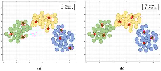
Figure 1.
Schematic illustration of anchors and pixels distributions. Taking three clusters as an example, the dots and stars represent pixels and anchors, respectively, with different colored dots denoting distinct clusters. In Figure 1a, without considering the distribution of anchors and pixels, the anchors are affected by outliers and deviate from the pixels distribution, making it difficult to accurately represent the pixels. In Figure 1b, the anchors maintain the distribution of the pixels and better represent the pixels under the constraint of distributed consistency. (a) Inconsistency. (b) Consistency.
To combat the aforementioned issue, we propose a discriminative anchor learning method for hyperspectral image clustering. Within a self-expressive framework, our model explicitly aligns the anchors distribution with the pixels distribution by sharing the same coefficient matrix, enabling the learned anchors to better represent the pixels. We impose the low-rank regularization constraint on the consensus coefficient matrix to reveal the underlying low-dimensional subspace structure. Different from the classic subspace clustering algorithms that enforce the diagonal elements of the coefficient matrix which are zero and where the row sum is one, we apply non-negative and row-sum-to-one constraints on the coefficient matrix. The non-negativity constraint ensures positive contribution between anchors, eliminating interference from negative values in similarity judgments and enhancing interpretability. The row-sum-to-one constraint normalizes the relationships between each anchor and others. Under these dual constraints, the coefficients corresponding to intra-class anchors are more concentrated, while those for inter-class anchors are sparser, which strengthens the anchors’ discriminative ability. Using the anchor graph constructed from discriminative anchors can achieve superior clustering performance.
The primary contributions of this paper are as follows:
- We propose a discriminative anchor learning strategy to capture the intrinsic structure of anchors. By sharing the coefficient matrix, this strategy aligns the anchors distribution with the pixels distribution, facilitating the effective clustering.
- We impose low-rank and probabilistic constraints on the consensus coefficient matrix, which not only excavates the global structures but also enhances the discriminative capability of the anchors.
- We present an alternating optimization strategy to solve the proposed formulation. Extensive experimental results demonstrate the superiority and effectiveness of the proposed method.
2. Related Work
Driven by diverse clustering mechanisms, various HSI clustering algorithms have witnessed flourishing development. Among them, subspace-based clustering methods effectively model homogeneous land-covers using a single subspace and express the internal structure of HSI through the union of these subspaces. Given an HSI tensor with pixels and B bands, we reshape it into a matrix denoted by , where . Traditional SSC algorithms need to construct affinity matrix with computational complexity , which is not suitable for large-scale HSI clustering tasks. Table 1 details the main used notations and definitions in the paper.

Table 1.
Notations and definitions used throughout the paper.
To address this challenge, anchor-based strategies are employed to construct a similarity matrix. For instance, Wang et al. proposed a non-negative relaxation-based graph clustering method, which utilized an anchor graph to accelerate the calculation process and mitigated computational overhead [32]. By enforcing orthogonal non-negative constraints on the category indicator matrix, it eliminates the need for K-means and directly outputs the clustering results. Due to the influence of the continuity of ground objects, adjacent pixels exhibit significant correlation in spectral features. Taking this problem into account, Wang et al. presented a fast spectral clustering with anchor graph by incorporating spatial information [33]. It applies mean filtering to obtain denoised pixels that incorporate contextual information, and then constructs a shared anchor graph based on these pixels and original pixels for clustering. Given that HSI contains uniform regions of varying sizes, single-scale filtering cannot accurately cover local uniform areas. Wang et al. proposed a spatial–spectral clustering with anchor graph, which enhances the consistency of pixels within local windows through multi-scale mean filtering, obtaining more representative characteristics [34]. Considering that the pixels within each generated superpixel share identical features, Chen et al. proposed a spectral–spatial superpixel anchor graph-based clustering method [35]. By integrating spatial and structural information as well as superpixel-based anchor selection strategies, the clustering performance is further boosted. To achieve more efficient clustering, Cai et al. developed a neighborhood contrastive subspace clustering network, which utilizes a superpixel pooling autoencoder to learn subspace representations at the superpixel level for clustering [36]. To integrate spectral, spatial, and structural information, Zhang et al. constructed a superpixel graph and a band graph based on superpixel features, and realized elastic graph fusion subspace clustering through three effective graph fusion strategies [37]. Taking the superpixels obtained via SLIC segmentation as input, Luo et al. proposed a self-supervised double-structure transformer. It jointly optimizes a shared autoformer structure based on the autoencoder and transformer and Siamese dual-former graph structure for HSI clustering [19]. Guan et al. mined deep spectral and spatial information as two branches via graph autoencoders, utilized cluster-oriented consistency learning to generate consistent distributions for nodes, and finally adopted hard sample contrastive learning to better focus on indistinguishable samples, thereby enhancing discriminative capability [17]. Although these methods have exhibited excellent performance on some datasets, their anchors are fixed after initialization. This setting is not flexible, making it difficult to obtain an appropriate similarity matrix in practical applications.
To solve this problem, adaptive anchors learning algorithms have been proposed. Huang et al. learned a compact dictionary from data to model the low-dimensional subspaces [24]. Considering that uniform regions exhibit greater spatial continuity than edge regions, this algorithm adopted an adaptive spatial regularization for the representation coefficients, achieving superior clustering performance. Although this method achieves favorable clustering performance, it separates feature learning and clustering tasks into two stages, resulting in suboptimal clustering results. Inspired by matrix factorization, Zhang et al. directly obtained the clustering labels of sampled data through two rounds of matrix factorization on pixel subsets, and then used a K-nearest neighbor classifier to derive the labels of all pixels [38]. Zhang et al. proposed a bipartite graph-based projection clustering algorithm, which incorporates projection learning and bipartite graph learning with explicit connected components into a unified framework, obtaining the clustering results in one step [29]. It is worth noting that when the number of pixels is extremely large, learning the clustering structure from pixel-anchor graph remains a time-consuming process. For this reason, Jiang et al. developed structured anchor-based projected clustering [39]. It simultaneously learns a pixel-anchor graph and an anchor–anchor graph with Laplacian rank constraint within the projection space. Based on these two graphs, the model propagates clustering labels from anchors to pixels, accomplishing the clustering of original HSI. To consider the symmetry condition of graph during the process of affinity estimation, Wang et al. proposed a doubly stochastic graph based projected clustering [40]. Introducing the doubly stochastic constraints results in learning an anchor–anchor graph with strict probabilistic affinity, which directly provides anchor cluster indicators via connectivity. Subsequently, label propagation is employed to derive pixel-level clustering results. Although the aforementioned methods have achieved satisfactory clustering performance, they fail to consider anchors distribution during anchor selection, resulting in suboptimal anchors, which consequently compromises the performance of subsequent clustering tasks. Therefore, we propose a discriminative anchor-based hyperspectral image clustering algorithm. By considering the consistent similarity distribution between anchors and pixels, more representative anchors are obtained to improve the quality of anchor images.
3. Methodology
3.1. Problem Formulation and Objective Function
For anchor-based clustering algorithms, the selection of high-quality anchors is a pivotal challenge. Although the existing methods have achieved good performance, they directly utilize the learned anchors for clustering, overlooking the distribution consistency between anchors and samples. To address this problem, our approach integrates spectral, spatial, and distribution information to learn high-quality anchors. Then, the pixel-anchor graph constructed from discriminative anchors is used for clustering.
Superpixel Generation. Generally speaking, pixels belonging to the same class are mostly distributed within homogeneous regions. Entropy rate superpixel (ERS) segmentation [41] techniques can adaptively generate such homogeneous regions based on the spatial distribution and texture information of pixels, offering a viable approach to extract spectral–spatial structures. ERS is initially designed for RGB image segmentation, which requires converting the RGB image into a grayscale image and then segmenting the grayscale image. Given that hyperspectral remote sensing images comprise numerous spectral bands, we need to select a representative component to perform segmentation. Principal component analysis (PCA) is a common dimension reduction technique and is widely employed for data preprocessing in ERS segmentation. In detail, we adopt the max-min normalization to standardize the features to eliminate the impact of feature magnitude differences on PCA. Only the first principal component (PCA dimensionality = 1) is retained for executing ERS to obtain M non-overlapping superpixels as
where is the i-th superpixel. By mapping the segmentation results back to the original HSI, we obtain the corresponding superpixels across all spectral bands.
Each superpixel contains pixels, denoted as . The i-th anchor is computed by averaging the pixels within the same superpixel, i.e.,
where . Based on M superpixels, we derive the initialized anchor matrix .
Spatial Denoising. In the acquisition of hyperspectral images, noise and outliers are inevitably introduced, which degrades image quality and affects subsequent clustering tasks. To mitigate the influence of noise and outliers, most existing algorithms augment spatial information by implementing mean filtering within small square windows. Nevertheless, such an approach is too strict to effectively extract complex spatial features. Considering that superpixel segmentation can generate homogeneous regions, conducting denoising operations within the same superpixel can result in the desired denoised pixels. Given an original pixel within , we identify its K nearest spatial neighbors within the corresponding superpixel using the Euclidean distance and define them as . To accomplish effective denoising, we denoise by employing the weighted sum of K nearest neighbors, and the formula is expressed as
where is the denoised pixel of . The weight of the spectral similarity between and is denoted by
where and . By applying the above operation to all pixels, we can obtain the denoised image . Through noise suppression, we strengthen the spatial coherence of the image while boosting the representativeness of the data.
Discriminative Anchor Learning. The initialized anchor matrix incorporates the spatial consistency of the image, yet fails to account for the distribution consistency between anchors and pixels. Ideally, the anchors have a consensus distribution structure with the denoised pixels . If a pixel exhibits high affinity with certain anchors, these anchors have a high probability of belonging to the same cluster and the corresponding affinities are likely to be high as well. To achieve this, we jointly learn anchor matrix and anchor graph within a self-expression framework, allowing these two matrices to share the same coefficient representation for aligning the anchors with the pixels distribution. The loss function is
where is defined as an anchor graph. is the regularization term, , and are trade-off parameters. Since similar pixels usually produce similar representation coefficients, dissimilar pixels yield different representation coefficients, we can regard as the extracted features of input data . Under the self-representation model, we learn the coefficient matrix corresponding to the anchor matrix , which contains the anchor–anchor relationships. We further decompose the anchor graph into the anchor graph and the anchor coefficient matrix . Through the consistent coefficient matrix , we enhance the consistency between the affinity relationships among anchors and those between pixels and anchors, promoting that the anchor distribution is consistent with the pixels distribution. Building on the superpixel-averaged anchors, we iteratively update the anchor matrix through adaptive learning, fostering greater alignment between the distribution of anchors and pixels. This approach effectively mitigates the potential errors arising from initial superpixel segmentation, thereby enhancing the quality of the anchors.
To explore the global low-rank structure, we impose a nuclear norm constraint on the coefficient matrix , which encourages a more desirable block structure. Moreover, by constraining the coefficient matrix to be non-negative with row sums equal to one, the coefficient representations of intra-class anchors are more compact, while those of inter-class anchors are more dispersed. This further enhances the anchors’ discriminative capability. The final objective function is as follows:
where is a nuclear norm that represents the sum of all non-zero singular values in the matrix.
3.2. Optimization
It is challenging to directly address the model (6) when all variables are considered at once. Based on Augmented Lagrange Multiplier [42], we introduce the following auxiliary variables , and . By setting and , the model (6) can be rewritten as
where , , and represent Lagrange multipliers; , , and are the penalty parameters. The problem (7) can be solved by an alternating optimization method.
-subproblem. Fixing the variables , , , and . In this condition, the optimization of is
Taking the derivative of Equation (8) w.r.t and setting it to zero, can be updated by
-subproblem. Fixing the variables , , , and . In this condition, the optimization of is
Taking the derivative of Equation (10) w.r.t and setting it to zero, can be updated by
-subproblem. Fixing the variables , , , and . In this condition, the optimization of is
Taking the derivative of Equation (12) w.r.t and setting it to zero, can be updated by
-subproblem. Fixing the variables , , , and . In this condition, the optimization of is
In order to solve the issue, we present the following theorem.
Theorem 1
([43]). Suppose an arbitrary matrix and it is decomposed into , , , . For the following optimization problem
the optimal solution is
where , which can be calculated by the soft-thresholding method [44].
According to Theorem 1, can be updated by
-subproblem. Fixing the variables , , , and . In this condition, the optimization of is
where . Based on [45], the closed-form solution of is
where and stands for the Lagrangian multiplier.
-subproblem. Fixing the variables , , , and . In this condition, the optimization of is
where . Based on [45], the closed-form solution of is
where is the Lagrangian multiplier.
Furthermore, the Lagrange multipliers , , and can be updated as
The penalty parameters are updated by
where represents the given constant.
Ultimately, we encapsulate the pseudo code in Algorithm 1.
| Algorithm 1: Discriminative anchor learning for hyperspectral image clustering. |
Input: HSI matrix , number of superpixels M, parameters , and . |
Output: Clustering labels.
|
3.3. Complexity Analysis
Computational Complexity. The computational consumption of the proposed algorithm comprises two phases: HSI segmentation and optimization by iteratively solving Equation (6). To achieve HSI segmentation, it requires for performing PCA and takes for conducting ERS. Subsequently, we concentrate on optimizing six variables, i.e., , , , , and . To optimize the and subproblems, they take at each iteration. As for the and subproblems, they need and at each iteration, respectively. Updating and take , and , respectively. Since , the primary computational complexity of the proposed algorithm in each iteration is .
Storage Complexity. Throughout the optimization process, the storage consumption of the proposed method mainly originates from , , , , and . For these eight variables, their corresponding storage complexities are , , , , and . Thus, the storage complexity of the proposed algorithm is .
4. Experiments
4.1. Experiment Settings
Datasets. To evaluate our proposed method, we conducted extensive experiments on three commonly used HSI datasets, including Salinas, Pavia University (PaviaU), and Pavia Center (PaviaC) [29]. The detailed statistical information of these datasets is presented in Table 2.
Table 2.
HSI datasets utilized in this paper.
Baselines. To demonstrate the effectiveness of our proposed method, we compare it with several representative clustering methods. FSCAG [33]: Constructing an anchor graph separately based on the original pixels and denoised pixels via mean filtering and performing fast spectral clustering to get the clustering labels. HESSC [46]: Automatically estimating the number of clusters and executing hierarchical sparse subspace clustering. NCSC [36]: Designing a superpixel pooling autoencoder to learn superpixel-level subspace representations and employing neighborhood contrastive regularization to enhance the robustness of subspace representations. S3AGC [35]: Building an anchor graph using denoised pixels and band structure information, followed by spectral clustering on similarity matrix to obtain the clustering results. BGPC [29]: Combining projection learning and bipartite graph learning with Laplacian rank constraint into a unified framework to directly obtain the clustering outcomes. SDST [19]: Designing a self-supervised double-structure transformer that contains a shared autoformer and Siamese dual-former graph module to enhance the representation performance of features for clustering. SSGCC [17]: Designing a spatial–spectral graph contrastive clustering that dynamically set the weights of sample pairs, enabling the model to prioritize handling hard samples. SAPC [39]: Learning a pixel-anchor graph and an anchor–anchor graph with Laplacian rank constraint in the projection space and designing an inference strategy to derive the clustering labels. HPCDL [40]: Imposing doubly stochastic constraints on an anchor–anchor graph and producing a better graph with strict probabilistic affinity. For a more intuitive comparison, we summarized the above algorithm from four aspects: parameter sharing, stochastic, regularization, and end-to-end, as shown in Table 3.
Table 3.
Mechanism comparison table of different compared methods.
Experimental Settings.
To ensure an equitable comparison between the proposed method and the baselines, NCSC, SDST, and SSGCC are implemented on a standard Windows 10 Server with two Intel(R) Xeon(R) Platinum 8168 CPUs 2.7 GHz and 384 GB RAM. The remaining experiments are conducted using MATLAB 2020b. To quantify the clustering performance, we adopt five common metrics in HSI clustering methods, including overall clustering accuracy (OA), average clustering accuracy (AA), Kappa coefficient, normalized mutual information (NMI), and Purity. Higher values in all metrics reflect better clustering performance.
To determine the homogeneous regions, we adaptively set the number of superpixels by
where denotes the number of nonzero elements in the detected edge image, and is an adjustable parameter whose default is 2000. M is finely adjusted within the range of [100 200] to obtain a more suitable homogeneous area. To achieve optimal clustering results, we employ a grid search strategy to fine-tune the parameters included in the proposed model. Specifically, we adjust the parameters , and in the range of [0.01 100]. Each experiment is repeated 10 times, and the outcomes are presented as an average.
4.2. Experimental Results and Analysis
Performance Comparison. Table 4 presents the experimental results of different clustering methods on three HSI datasets. Bold and underline are used to highlight the best and second-best results for all methods, respectively. By observing and analyzing the extensive experimental results, it can be seen that our method has achieved better clustering performance compared with most comparative algorithms. Relative to the corresponding second-best baseline, our algorithm exhibits the obvious improvement of 8.4%, 2.6%, and 7.1% in OA, AA, and Kappa on the Salinas dataset. And our approach demonstrates the apparent promotion of 8.3%, 11.9%, and 17.8% in OA, AA and Kappa over the second-best baseline on the PaviaU dataset.
Table 4.
Clustering performance on the Salinas, PaviaU, and PaviaC datasets.
To be specific, HESSC yields the poorest clustering results among all the comparative algorithms. This is because it only relies on spectral information for clustering and ignores the spatial information that is crucial for HSI clustering. By incorporating spatial information, FSCAG and S3AGC achieve better clustering performance compared to HESSC. For deep learning algorithms, NCSC, SDST and SSGCC have achieved better feature representation due to their complex network design, gaining promising clustering performance. Among these methods, constrained by the pixel–superpixel relationships, the superpixel-based method NCSC exhibits inferior clustering performance. Compared with shallow methods, these deep algorithms have poorer interpretability and higher computational complexity. In contrast to the aforementioned baselines, BGPC, SAPC, and HPCDL demonstrate superior clustering performance. This is primarily because BGPC can directly obtain pixel labels in one step, whereas SAPC and HPCDL can propagate anchor labels to pixels utilizing graph-based mechanisms, effectively realizing clustering tasks. By contrast, our proposed algorithm yields the optimal clustering performance. This superiority can be attributed to the consideration of anchor distribution during the anchor selection process. When the anchor distribution aligns with that of the pixels, it helps to generate more discriminative anchors. Remarkably, even when post-processing techniques such as K-means are applied to attain clustering labels, it still maintains excellent clustering performance. To visualize the clustering effect, the clustering maps obtained by different methods are presented in Figure 2, Figure 3 and Figure 4. From these figures, it can be observed that the clustering maps produced by the proposed algorithm are close to the ground truth maps. This further substantiates the superiority of our proposed algorithm.
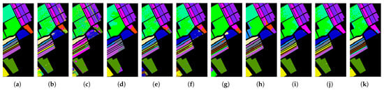
Figure 2.
Clustering maps on the Salinas dataset. (a) GT. (b) FSCAG. (c) HESSC. (d) NCSC. (e) S3AGC. (f) BGPC. (g) SDST. (h) SSGCC. (i) SAPC. (j) HPCDL. (k) OUR.
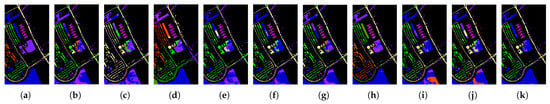
Figure 3.
Clustering maps on the PaviaU dataset. (a) GT. (b) FSCAG. (c) HESSC. (d) NCSC. (e) S3AGC. (f) BGPC. (g) SDST. (h) SSGCC. (i) SAPC. (j) HPCDL. (k) OUR.
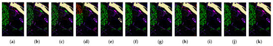
Figure 4.
Clustering maps on the PaviaC dataset. (a) GT. (b) FSCAG. (c) HESSC. (d) NCSC. (e) S3AGC. (f) BGPC. (g) SDST. (h) SSGCC. (i) SAPC. (j) HPCDL. (k) OUR.
t-SNE visualization. Figure 5 illustrates the clustering results visualized with t-distributed stochastic neighbor embedding (t-SNE) on the three HSI datasets. Each pixel is displayed using t-SNE, and distinct colors represent different cluster labels derived from our method. It can be observed that the proposed method exhibits better separability. Pixels within the same cluster are more aggregated, while those from different clusters are further dispersed, obtaining more discriminative representations.
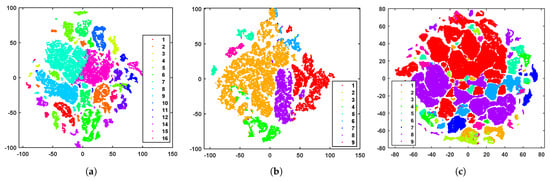
Figure 5.
Visualization of the clustering results with t-SNE on the three datasets. (a) Salinas. (b) PaviaU. (c) PaviaC.
Parameter Study.
- Parameter M. We investigate the effect of M for our algorithm and record the clustering performance results (OA, NMI, and Kappa) as shown in Figure 6. Overall, the proposed method reaches the optimal outcomes when M is set to [120 200]. Furthermore, we can discover that these metrics curves do not monotonically increase with M. This implies that it is unnecessary to employ numerous anchors for clustering.
- Parameters , and . To facilitate observation, we analyze the effect of the parameters and for our method when is fixed. The results are shown in the first row of Figure 7. It can be observed that as and are varied, OA exhibits significant fluctuations, indicating that these parameters need to be carefully adjusted to optimize the clustering performances. Satisfactory clustering results are typically achieved when and are set within the range [0.1, 10]. The second row of Figure 7 shows the variation curve corresponding to . Obviously, the clustering results are notably impacted by these parameters, especially for the Salinas and PaviaU datasets. Because of the discrepancy in the distribution of dataset, different parameters are selected to achieve the optimal clustering results. When is set to 1, our method achieves the optimal clustering results on the Salinas and PaviaC datasets. And when is set to 100, our method achieves the optimal clustering results on the PaviaU dataset.

Figure 6.
Clustering performance with different M on the three datasets. (a) Salinas. (b) PaviaU. (c) PaviaC.

Figure 7.
Sensitivity analysis of the parameters , and on the three datasets. Left: Salinas; Medium: PaviaU; Right: PaviaC.
Effectiveness of ERS Segmentation.
Table 5 shows the comparison of different superpixel segmentation methods included SLIC, LSC and ERS. The performance of ERS incorporating spatial information outperforms SLIC and LSC. The main distinction lies in the fact that ERS embraces the complete spatial context, while SLIC and LSC rely on K-nearest neighbors for segmentation. By enhancing spatial awareness and more accurately capturing spatial relationships within the data, ERS achieves improved clustering accuracy.
Table 5.
Ablation study of segmentation algorithms.
Ablation Study. To demonstrate the effectiveness of discriminative anchors (DAs) and low-rank constraint (LR) in our proposed algorithm, we conduct ablation experiments on the three HSI datasets, as shown in Table 6. DA and LR respectively correspond to the third and fourth terms in the objective function. By comparing three variants, we find that explicitly learning discriminative anchors and low-rank constraint can better represent pixels, improving the quality of anchor graph and enhancing the clustering performance.
Table 6.
Ablation study of the proposed method on the three datasets.
Converge Analysis. For the proposed method, we set the iteration cap to 300. When the reconstruction errors (i.e., , and ) are less than , the iteration stops and the model converges. To investigate the convergence of the proposed algorithm, we plot the convergence curves of reconstruction errors and clustering metrics curves (OA, NMI, and Kappa) on the three databases in Figure 8. It can be seen that our algorithm can gradually converge within 100 iterations, and the best performance after convergence is selected as the final metric. Therefore, our algorithm has good convergence and performs well in practical applications.
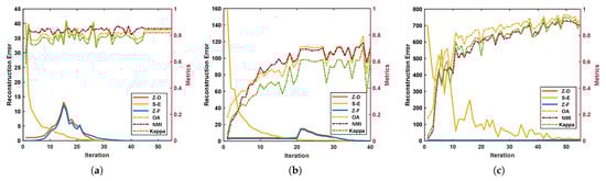
Figure 8.
Convergence curves and clustering metrics curves on the three datasets. (a) Salinas. (b) PaviaU. (c) PaviaC.
5. Conclusions
In this paper, we proposed a discriminative anchor-based HSI clustering algorithm. It achieves consistency between the distribution of anchors and that of pixels by sharing the coefficient matrix between an anchor matrix and anchor graph, ensuring that the selected anchors can better reflect the distribution structure of pixels. By imposing low-rank and probabilistic constraints on the consensus coefficient matrix, it effectively excavates the structural information of anchors and strengthens their discriminative ability. Experimental results on three HSI databases have confirmed the superiority and effectiveness of the proposed approach.
Author Contributions
Conceptualization, Y.Y. and Q.G.; methodology, Y.Y. and Q.G.; software, Y.Y.; validation, J.Z., Y.D. and C.D.; visualization, Y.Y., J.Z. and Y.D.; supervision, Q.G., J.Z., Y.D. and C.D.; project administration, Q.G., J.Z. and Y.D.; data curation, Y.Y., J.Z. and Y.D.; writing—original draft preparation, Y.Y.; writing—review and editing, Y.Y., Q.G., J.Z. and Y.D. All authors have read and agreed to the published version of the manuscript.
Funding
This work was supported by the National Natural Science Foundation of China, Grant No. 62176203 and 62576263; the Natural Science Basic Research Program of Shaanxi Province, Grant No. 2025JC-QYCX-051; and the Fundamental Research Funds for the Central Universities and the Innovation Fund of Xidian University, Grant No. YJSJ25007.
Data Availability Statement
The data presented in this study are available on request corresponding author.
Conflicts of Interest
The authors declare no conflicts of interest.
References
- Yang, G.; Huang, K.; Sun, W.; Meng, X.; Mao, D.; Ge, Y. Enhanced mangrove vegetation index based on hyperspectral images for mapping mangrove. ISPRS J. Photogramm. Remote Sens. 2022, 189, 236–254. [Google Scholar] [CrossRef]
- Tu, B.; He, W.; Li, Q.; Peng, Y.; Plaza, A. A New Context-Aware Framework for Defending Against Adversarial Attacks in Hyperspectral Image Classification. IEEE Trans. Geosci. Remote Sens. 2023, 61, 5505114. [Google Scholar] [CrossRef]
- Zhang, B.; Li, S.; Wu, C.; Gao, L.; Zhang, W.; Peng, M. A neighbourhood-constrained k-means approach to classify very high spatial resolution hyperspectral imagery. Remote Sens. Lett. 2013, 4, 161–170. [Google Scholar] [CrossRef]
- Ranjan, S.; Nayak, D.R.; Kumar, K.S.; Dash, R.; Majhi, B. Hyperspectral image classification: A k-means clustering based approach. In Proceedings of the 2017 4th International Conference on Advanced Computing and Communication Systems (ICACCS), Coimbatore, India, 6–7 January 2017; pp. 1–7. [Google Scholar]
- Ghaffarian, S.; Ghaffarian, S. Automatic histogram-based fuzzy C-means clustering for remote sensing imagery. ISPRS J. Photogramm. Remote Sens. 2014, 97, 46–57. [Google Scholar] [CrossRef]
- Rodriguez, A.; Laio, A. Clustering by fast search and find of density peaks. Science 2014, 344, 1492–1496. [Google Scholar] [CrossRef]
- Ester, M.; Kriegel, H.-P.; Sander, J.; Xu, X. A Density-Based Algorithm for Discovering Clusters in Large Spatial Databases with Noise. In Proceedings of the International Conference on Knowledge Discovery and Data Mining (KDD-96), Portland, OR, USA, 2–4 August 1996; pp. 226–231. [Google Scholar]
- Xie, H.; Zhao, A.; Huang, S.; Han, J.; Liu, S.; Xu, X.; Luo, X.; Pan, H.; Du, Q.; Tong, X. Unsupervised Hyperspectral Remote Sensing Image Clustering Based on Adaptive Density. IEEE Geosci. Remote Sens. Lett. 2018, 15, 632–636. [Google Scholar] [CrossRef]
- Zhao, Y.; Yuan, Y.; Wang, Q. Fast Spectral Clustering for Unsupervised Hyperspectral Image Classification. Remote Sens. 2019, 11, 399. [Google Scholar] [CrossRef]
- Huang, N.; Xiao, L.; Liu, J.; Chanussot, J. Graph Convolutional Sparse Subspace Coclustering With Nonnegative Orthogonal Factorization for Large Hyperspectral Images. IEEE Trans. Geosci. Remote Sens. 2023, 60, 5512016. [Google Scholar] [CrossRef]
- Cai, Y.; Zeng, M.; Cai, Z.; Liu, X.; Zhang, Z. Graph Regularized Residual Subspace Clustering Network for Hyperspectral Image Clustering. Inf. Sci. 2021, 578, 85–101. [Google Scholar] [CrossRef]
- Li, T.; Cai, Y.; Zhang, Y.; Cai, Z.; Liu, X. Deep Mutual Information Subspace Clustering Network for Hyperspectral Images. IEEE Geosci. Remote Sens. Lett. 2022, 19, 6009905. [Google Scholar] [CrossRef]
- Lei, J.; Li, X.; Peng, B.; Fang, L.; Ling, N.; Huang, Q. Deep Spatial-Spectral Subspace Clustering for Hyperspectral Image. IEEE Trans. Circuits Syst. Video Technol. 2021, 31, 2686–2697. [Google Scholar] [CrossRef]
- Zhao, Y.; Li, X. Deep Spectral Clustering With Regularized Linear Embedding for Hyperspectral Image Clustering. IEEE Trans. Geosci. Remote Sens. 2023, 61, 5509311. [Google Scholar] [CrossRef]
- Zhang, Y.; Wang, Y.; Chen, X.; Jiang, X.; Zhou, Y. Spectral–Spatial Feature Extraction With Dual Graph Autoencoder for Hyperspectral Image Clustering. IEEE Trans. Circuits Syst. Video Technol. 2022, 32, 8500–8511. [Google Scholar] [CrossRef]
- Hu, X.; Li, T.; Zhou, T.; Peng, Y. Deep Spatial-Spectral Subspace Clustering for Hyperspectral Images Based on Contrastive Learning. Remote Sens. 2021, 13, 4418. [Google Scholar] [CrossRef]
- Guan, R.; Tu, W.; Li, Z.; Yu, H.; Hu, D.; Chen, Y.; Tang, C.; Yuan, Q.; Liu, X. Spatial–Spectral Graph Contrastive Clustering With Hard Sample Mining for Hyperspectral Images. IEEE Trans. Geosci. Remote Sens. 2024, 62, 5535216. [Google Scholar] [CrossRef]
- Liu, W.; Liu, K.; Sun, W.; Yang, G.; Ren, K.; Meng, X.; Peng, J. Self-Supervised Feature Learning Based on Spectral Masking for Hyperspectral Image Classification. IEEE Trans. Geosci. Remote Sens. 2023, 61, 4407715. [Google Scholar] [CrossRef]
- Luo, F.; Liu, Y.; Duan, Y.; Guo, T.; Zhang, L.; Du, B. SDST: Self-Supervised Double-Structure Transformer for Hyperspectral Images Clustering. IEEE Trans. Geosci. Remote Sens. 2024, 62, 5511614. [Google Scholar] [CrossRef]
- Elhamifar, E.; Vidal, R. Sparse Subspace Clustering: Algorithm, Theory, and Applications. IEEE Trans. Pattern Anal. Mach. Intell. 2013, 35, 2765–2781. [Google Scholar] [CrossRef]
- Zhang, H.; Zhai, H.; Zhang, L.; Li, P. Spectral-Spatial Sparse Subspace Clustering for Hyperspectral Remote Sensing Images. IEEE Trans. Geosci. Remote Sens. 2016, 54, 3672–3684. [Google Scholar] [CrossRef]
- Zhai, H.; Zhang, H.; Zhang, L.; Li, P.; Plaza, A. A New Sparse Subspace Clustering Algorithm for Hyperspectral Remote Sensing Imagery. IEEE Geosci. Remote Sens. Lett. 2017, 14, 43–47. [Google Scholar] [CrossRef]
- Cai, Y.; Zhang, Z.; Cai, Z.; Liu, X.; Jiang, X.; Yan, Q. Graph convolutional subspace clustering: A robust subspace clustering framework for hyperspectral image. IEEE Trans. Geosci. Remote Sens. 2021, 59, 4191–4202. [Google Scholar] [CrossRef]
- Huang, S.; Zhang, H.; Pizurica, A. Subspace clustering for hyperspectral images via dictionary learning with adaptive regularization. IEEE Trans. Geosci. Remote Sens. 2022, 60, 5524017. [Google Scholar] [CrossRef]
- Zhai, H.; Zhang, H.; Zhang, L.; Li, P. Sparsity-Based Clustering for Large Hyperspectral Remote Sensing Images. IEEE Trans. Geosci. Remote Sens. 2021, 59, 10410–10424. [Google Scholar] [CrossRef]
- Huang, S.; Zeng, H.; Chen, H.; Zhang, H. Spatial and Cluster Structural Prior-Guided Subspace Clustering for Hyperspectral Image. IEEE Trans. Geosci. Remote Sens. 2024, 62, 5511115. [Google Scholar] [CrossRef]
- Huang, S.; Zhang, H.; Du, Q.; Pizurica, A. Sketch-Based Subspace Clustering of Hyperspectral Images. Remote Sens. 2020, 12, 775. [Google Scholar] [CrossRef]
- Zhai, H.; Zhang, H.; Zhang, L.; Li, P. Nonlocal Means Regularized Sketched Reweighted Sparse and Low-Rank Subspace Clustering for Large Hyperspectral Images. IEEE Trans. Geosci. Remote Sens. 2021, 59, 4164–4178. [Google Scholar] [CrossRef]
- Zhang, Y.; Jiang, G.; Cai, Z.; Zhou, Y. Bipartite Graph-Based Projected Clustering With Local Region Guidance for Hyperspectral Imagery. IEEE Trans. Multim. 2024, 26, 9551–9563. [Google Scholar] [CrossRef]
- Zhao, H.; Zhou, F.; Bruzzone, L.; Guan, R.; Yang, C. Superpixel-level Global and Local Similarity Graph-based Clustering for Large Hyperspectral Images. IEEE Trans. Geosci. Remote Sens. 2022, 60, 5519316. [Google Scholar] [CrossRef]
- Cui, K.; Li, R.; Polk, S.L.; Lin, Y.; Zhang, H.; Murphy, J.M.; Plemmons, R.J.; Chan, R.H. Superpixel-based and Spatially-regularized Diffusion Learning for Unsupervised Hyperspectral Image Clustering. IEEE Trans. Geosci. Remote Sens. 2024, 62, 4405818. [Google Scholar] [CrossRef]
- Wang, R.; Nie, F.; Wang, Z.; He, F.; Li, X. Scalable Graph-Based Clustering With Nonnegative Relaxation for Large Hyperspectral Image. IEEE Trans. Geosci. Remote Sens. 2019, 57, 7352–7364. [Google Scholar] [CrossRef]
- Wang, R.; Nie, F.; Yu, W. Fast Spectral Clustering With Anchor Graph for Large Hyperspectral Images. IEEE Geosci. Remote Sens. Lett. 2017, 14, 2003–2007. [Google Scholar] [CrossRef]
- Wang, Q.; Miao, Y.; Chen, M.; Yuan, Y. Spatial-Spectral Clustering With Anchor Graph for Hyperspectral Image. IEEE Trans. Geosci. Remote Sens. 2022, 60, 5542413. [Google Scholar] [CrossRef]
- Chen, X.; Zhang, Y.; Feng, X.; Jiang, X.; Cai, Z. Spectral-Spatial Superpixel Anchor Graph-Based Clustering for Hyperspectral Imagery. IEEE Geosci. Remote Sens. Lett. 2023, 20, 5507405. [Google Scholar] [CrossRef]
- Cai, Y.; Zhang, Z.; Ghamisi, P.; Ding, Y.; Liu, X.; Cai, Z.; Gloaguen, R. Superpixel Contracted Neighborhood Contrastive Subspace Clustering Network for Hyperspectral Images. IEEE Trans. Geosci. Remote Sens. 2021, 60, 5530113. [Google Scholar] [CrossRef]
- Zhang, Y.; Wang, X.; Jiang, X.; Zhang, L.; Du, B. Elastic Graph Fusion Subspace Clustering for Large Hyperspectral Image. IEEE Trans. Circuits Syst. Video Technol. 2025, 35, 6300–6312. [Google Scholar] [CrossRef]
- Zhang, L.; Zhang, L.; Du, B.; You, J.; Tao, D. Hyperspectral image unsupervised classification by robust manifold matrix factorization. Inf. Sci. 2019, 485, 154–169. [Google Scholar] [CrossRef]
- Jiang, G.; Zhang, Y.; Wang, X.; Jiang, X.; Zhang, L. Structured Anchor Learning for Large-Scale Hyperspectral Image Projected Clustering. IEEE Trans. Circuits Syst. Video Technol. 2025, 35, 2328–2340. [Google Scholar] [CrossRef]
- Wang, N.; Cui, Z.; Lan, Y.; Zhang, C.; Xue, Y.; Su, Y.; Li, A. Large-Scale Hyperspectral Image-Projected Clustering via Doubly Stochastic Graph Learning. Remote Sens. 2025, 17, 1526. [Google Scholar] [CrossRef]
- Liu, M.-Y.; Tuzel, O.; Ramalingam, S.; Chellappa, R. Entropy rate superpixel segmentation. In Proceedings of the IEEE Conference on Computer Vision and Pattern Recognition (CVPR), Colorado Springs, CO, USA, 20–25 June 2011; pp. 2097–2104. [Google Scholar]
- Lin, Z.; Liu, R.; Su, Z. Linearized Alternating Direction Method with Adaptive Penalty for Low-Rank Representation. In Proceedings of the Advances in Neural Information Processing Systems 24 (NIPS 2011), Granada, Spain, 12–15 December 2011; pp. 612–620. [Google Scholar]
- Gao, Q.; Zhang, P.; Xia, W.; Xie, D.; Gao, X.; Tao, D. Enhanced Tensor RPCA and Its Application. IEEE Trans. Pattern Anal. Mach. Intell. 2021, 43, 2133–2140. [Google Scholar] [CrossRef]
- Cai, J.-F.; Candès, E.J.; Shen, Z. A singular value thresholding algorithm for matrix completion. SIAM J. Optim. 2010, 20, 1956–1982. [Google Scholar] [CrossRef]
- Nie, F.; Wang, X.; Jordan, M.; Huang, H. The constrained laplacian rank algorithm for graph-based clustering. In Proceedings of the AAAI Conference on Artificial Intelligence, Phoenix, AZ, USA, 12–17 February 2016; pp. 1969–1976. [Google Scholar]
- Shahi, K.R.; Khodadadzadeh, M.; Tusa, L.; Ghamisi, P.; Tolosana-Delgado, R.; Gloaguen, R. Hierarchical Sparse Subspace Clustering (HESSC): An Automatic Approach for Hyperspectral Image Analysis. Remote Sens. 2020, 12, 2421. [Google Scholar] [CrossRef]
Disclaimer/Publisher’s Note: The statements, opinions and data contained in all publications are solely those of the individual author(s) and contributor(s) and not of MDPI and/or the editor(s). MDPI and/or the editor(s) disclaim responsibility for any injury to people or property resulting from any ideas, methods, instructions or products referred to in the content. |
© 2025 by the authors. Licensee MDPI, Basel, Switzerland. This article is an open access article distributed under the terms and conditions of the Creative Commons Attribution (CC BY) license (https://creativecommons.org/licenses/by/4.0/).