Article

Assessment of WRF-Solar and WRF-Solar EPS Radiation Estimation in Asia Using the Geostationary Satellite Measurement

State Key Laboratory of Severe Weather Meteorological Science and Technology & Key Laboratory of Atmospheric Chemistry of CMA, Chinese Academy of Meteorological Sciences, Beijing 100081, China
*
Author to whom correspondence should be addressed.
Remote Sens. 2025, 17(24), 3970; https://doi.org/10.3390/rs17243970
Submission received: 6 November 2025 / Revised: 4 December 2025 / Accepted: 5 December 2025 / Published: 9 December 2025

Highlights

What are the main findings?
  • The WRF-Solar EPS model shows comparable short-term (<36 h) forecasting capabilities to WRF-Solar, the model performing well in the Beijing-Tianjin-Hebei region and the Yangtze River Delta. Bias is lower in summer and autumn, while RMSE and MAE are lower in autumn and winter.
  • There is a temporal mismatch in the seasonal fluctuations of the bias, root mean square error, and mean absolute error of GHI. The errors fluctuations in DIR over Western China follow a distinctive pattern.
What are the implications of the main findings?
  • Ensemble forecasting can slightly enhance the stability of forecast results, but improve results little in short-term forecasting.
  • The error performance of WRF-Solar and WRF-Solar EPS in the short-term prediction of solar irradiance at the interannual scale in Asia is quantitatively evaluated, which provides a basic reference for subsequent improvement work.

Abstract

Accurate solar radiation forecasting with numerical weather prediction (NWP) is critical for optimizing photovoltaic power generation. This study evaluates short-term (<36 h) performance of the Weather Research and Forecasting model (WRF-Solar) and its ensemble version (WRF-Solar EPS) for global horizontal irradiance (GHI) and direct horizontal irradiance (DIR) over East Asia (December 2019–November 2020) against geostationary satellite retrievals. Both models effectively capture GHI spatial patterns but exhibit systematic overestimation (biases: 17.27–17.68 W/m2), with peak errors in northwest China and the North China Plain. Temporal mismatches between bias (maximum in winter-spring) and RMSE/MAE (maximum in summer) may indicate seasonal variability in error signatures dominated by aerosols and clouds. For DIR, regional biases prevail: overestimation in the Tibetan Plateau and northwest China, and underestimation in southern China and Indo-China Peninsula. Errors (RMSE and MAE) are larger than for GHI, with peaks in southeast and northwest China, likely linked to poor cloud–aerosol simulations. WRF-Solar EPS shows no significant bias reduction but modest RMSE/MAE improvements in summer–autumn, particularly in southeast China, indicating limited enhancement of short-term predictive stability. Both WRF-Solar and WRF-Solar EPS require further refinements in cloud–aerosol parameterizations to mitigate systematic errors over East Asia in future applications.

1. Introduction

Faced with the increasing demand for photovoltaic power generation, forecasting for photovoltaic systems’ power output is essential for power plants and managers to plan generation capacity and improve electricity efficiency [1,2,3,4]. The essence of enhancing photovoltaic power forecasting lies in accurately obtaining surface solar radiation forecasts [5,6]. Various methods for solar radiation forecasting have been developed [7,8], such as all-sky cameras, satellite remote sensing retrievals [9,10], and numerical weather prediction (NWP). Statistical methods represented by machine learning and deep learning have also been extensively applied [11,12,13,14]. Among these, NWP models perform well in one-day forecasts due to the variability of solar radiation caused by clouds and microphysical processes, making it challenging for non-physics-based statistical methods to provide accurate forecasts over longer time scales (>6 h). However, general NWP models still lack sufficient consideration of the feedback of the interactions between aerosols and clouds on solar radiation, which can introduce uncertainty in solar radiation simulation. Therefore, to improve the accuracy of NWP solar radiation forecasts, a comprehensive analysis and validation of the traditional NWP model’s simulation is necessary.
Weather Research and Forecasting (WRF)-Solar model [15], as one of the representative NWP models, is specifically developed for photovoltaic power forecasting. Compared to conventional models, WRF-Solar incorporates several enhancements in radiation calculations [16], such as accounting for the radiative effects of atmospheric aerosols and improving the feedback of clouds on radiation. Research by [15] indicated that WRF-Solar significantly improves solar radiation forecasts under clear-sky conditions compared to the standard WRF model. Subsequent evaluations and studies of WRF-Solar performance have demonstrated its operational stability and reliability in photovoltaic power forecasting applications [17,18,19,20].
Ensemble forecasting can effectively reduce the forecast errors associated with a single forecast while generating probabilistic forecasts essential for grid operations. The WRF-Solar Ensemble Prediction System (WRF-Solar EPS) [21,22], an ensemble forecasting framework that generates multiple members by introducing stochastic perturbations to the input variables of the WRF-Solar physical parameterization schemes, is distinguished from WRF-Solar because of its implementation of a tangent linear analysis [23] to assess the influence of variables within the parameterization schemes on the simulation uncertainty. Several dominant parameters are selected and added random perturbations for the ensemble forecasts to further address critical requirements for probabilistic solar forecasting in photovoltaic plant scheduling and risk management.
The implementation of China’s dual-carbon policy has accelerated renewable energy deployment across East Asia, especially the installation of solar photovoltaic. This rapid transition emphasizes the critical need for reliable solar irradiance forecasting and monitoring. Although ground-based observations can provide high-precision in situ measurements, their spatial coverage is limited, making it difficult to capture the fine-scale spatial variations in solar irradiance, which are significantly influenced by clouds and aerosols. In contrast, geostationary satellite platforms, owing to their capability of delivering extensive, high spatiotemporal resolution remote sensing measurements, have become a crucial tool for current surface solar radiation monitoring. Ref. [24] proposed a method for deriving high-resolution solar irradiance data from Meteosat Second Generation (MSG) geostationary satellite and evaluated solar resources across Europe, highlighting the significant potential of applying remote sensing technologies to the solar energy industry. Ref. [25] developed the first freely available surface solar radiation database covering Asia using the Meteosat East geostationary satellite, aiding researchers and solar system planners in estimating photovoltaic system energy output. The updated version of The National Solar Radiation Data Base (NSRDB), developed by [26], through integration of Geostationary Operational Environmental Satellite (GOES) satellite remote sensing data, has been widely adopted in research and the energy industry and has been utilized to evaluate the overall performance of the WRF-Solar model across the contiguous United States. Recently, an optimal algorithm was developed to calculate several solar radiation compositions based on geostationary satellite measurements (Himawari-8/9 and Fengyun-4) under the full consideration of the effects of aerosol types and cloud phases [10,27]. At present, many studies have been discussed in the performance of WRF-Solar in East Asia. Ref. [28] applied satellite-retrieved AOD data to WRF-Solar and improved the model’s simulation of solar irradiance in North China during heavy haze period in winter. Ref. [29] evaluated a high-resolution model setup in East China and concluded that WRF-Solar outperforms the standard WRF model in simulating surface solar irradiance. The evaluation by [30] of WRF-Solar during a summer month in China also demonstrated the model’s advanced capabilities in solar irradiance simulation. Furthermore, there are many more studies on WRF-Solar focusing on cases [31,32,33]. However, there is still a lack of studies on the region for a longer time, such as the annual scale. Therefore, this study aims to assess the short-term predictive capabilities of WRF-Solar and WRF-Solar EPS across extended periods in East Asia, specifically in China using these high spatial-temporal resolution of radiation products derived from satellite measurements, which will deepen our understanding of WRF-Solar’s capabilities. The results are helpful for improving model performance in the region to enhance photovoltaic power forecasting. Our study consists of two model simulation experiments with specific details and data used, outlined in Section 2, and Section 3 presents the evaluation results. Discussion and conclusions are provided, respectively, in Section 4 and Section 5.

2. Materials and Methods

2.1. Satellite-Derived Solar Radiation Data

Due to the limited coverage of in situ ground-based measurement sites, this study employs global horizontal irradiance (GHI) and direct horizontal irradiance (DIR) products derived from the Himawari-8/9 and Fengyun-4A/B geostationary satellite measurements [27] to assess the WRF-Solar model’s simulated solar radiation. The products first employed the Himawari-8 cloud and haze mask (HCHM) algorithm developed by [34] to perform stringent and precise cloud and haze pixel detection and data screening of the satellite data. The cloud detection was accomplished using multi-band reflectance and brightness temperature information along with adaptive thresholds. The surface shortwave radiation components were then retrieved through an optimal algorithm that combines physically based radiative transfer modeling with machine learning techniques. This method comprehensively accounts for the effects of different aerosol types, cloud phase (water/ice), and atmospheric gases to achieve high retrieval accuracy. Validation against ground-based measurements from the seven sites in the Baseline Surface Radiation Network (BSRN) has shown that the products perform exceptionally well. For daily mean GHI, the relative root mean square error (rRMSE) is 10.94%, with a correlation coefficient (R) of 0.97, outperforming other products like CERES, ERA5, and GLASS [27].
The satellite data selected in this study cover December 2019 to November 2020 (2019-12-01T00:00 to 2020-11-30T23:00 UTC), temporally aligned with WRF-Solar hourly output. The model estimation and satellite products were well time-matched as the deletion of model estimation corresponding to satellite gaps and the linearly interpolation of satellite products into the same spatial resolution of model estimation.

2.2. WRF-Solar Setting

Because WRF-Solar is an NWP model specifically designed to provide relatively accurate solar irradiance forecasts for the photovoltaic power industry and also a special configuration based on the WRF. In this study, WRF-Solar and its ensemble forecasting version (WRF-Solar EPS) were employed based on the WRF version 4.5.2. The parametric physical process settings and optimal configurations in our study mainly refer to the reference configuration given in the Research Applications Laboratory from https://ral.ucar.edu/documentation/wrf-solar-reference-configuration (accessed on 4 May 2025) and the study of [35]. Two experiments were set up for WRF-Solar and WRF-Solar EPS to evaluate their simulated performance in East Asia, and the specific detailed configurations are summarized in Table 1.
In the WRF-Solar experimental setup, the Rapid Radiative Transfer Model for Global Circulation Models (RRTMG) was used for the longwave and shortwave radiation scheme [36], the Thompson was selected for the microphysics scheme [37], the Mellor-Yamada Nakanishi and Niino (MYNN) was selected for the planetary boundary layer scheme [38], the Noah was selected for the land surface parameterization scheme [39], the Grell-3D was selected for cumulus cloud parameterization scheme [40], and the climatological monthly AOD data was also used in all short-term forecast runs [41]. This choice aligns with our primary goal of evaluating the baseline performance of the standard WRF-Solar reference configuration from the Research Applications Laboratory. However, we acknowledge that the overly simplified AOD setting will impose certain limitations on model performance. The static climatological AOD data cannot capture the strong temporal and spatial variations in aerosol loading in East Asia, thereby introducing biases in the models’ solar irradiance forecasts. Employing time-varying, advanced AOD conditions to enhance the model performance will be a primary focus in further studies. It is noted that a sub-grid-scale cloud scheme (CL3) parameterized by relative humidity was included to account for radiative effects from unresolved clouds [42]. Ensemble simulations were generated by introducing stochastic perturbations to variables within the parameterization scheme, comprising eight member runs whose ensemble mean was subsequently calculated. The specific perturbation settings primarily follow those in [19] and the user guide from https://ral.ucar.edu/solutions/products/wrf-solar-eps (accessed on 4 May 2025), applying perturbation in different degrees according to the standard deviation to 13 model internal state variables. Perturbations were not added to the Deng shallow convection parameterization scheme; the perturbed parameterization schemes include microphysics, boundary layer, land surface, Fast-All-sky Radiation model, and CLD3 sub-grid cloud scheme.
The initial meteorological fields and boundary conditions for both simulation experiments were provided by forecast data from the National Centers for Environmental Prediction (NCEP) Global Forecast System (GFS), which has a horizontal resolution of 0.25° × 0.25° and temporal interval of 3 h. For assessing the annual performance of WRF-Solar and EPS short-term forecasts, according to the WRF-Solar experiment, we conducted 366 short-term simulations spanning 2019-11-30T12:00 to 2020-11-30T23:00 UTC. Each run was initiated at 12:00 UTC on the preceding day and finished at 23:00 UTC of the target date, with the initial 12 h spin-up period discarded from verification. The WRF-Solar EPS experiment was also conducted using this method, generating eight distinct ensemble simulation members by configuring perturbation fields. The model outputs data were generated at 1 h intervals and the simulated domain featured a two-nested grid system. (Figure 1): Domain_01 (d01) covers most of Asia with a horizontal resolution of 81 km, covering 149 × 119 grid points horizontally and a time step of 90 s. Domain_02 (d02) focuses on East Asia, particularly the Chinese region, with an enhanced resolution of 27 km, covering 276 × 192 grid points horizontally and a time step of 30 s. Both simulation domains employ identical physical parameterization scheme settings.

2.3. Statistics Methods

Several metrics including bias, root mean square error (RMSE), and mean absolute error (MAE) were employed to quantify discrepancies between the simulations of WRF-Solar and WRF-Solar EPS against the satellite-derived radiation products. The equations are described below.
b i a s = 1 N i = 1 N ( M o d e l i R e t r i e v a l i )
R M S E = 1 N i = 1 N M o d e l i R e t r i e v a l i 2
M A E = 1 N i = 1 N M o d e l i R e t r i e v a l i
Here, N denotes the total number of available NWP model outputs and satellite retrieval products covering the specified time range of the study. To further evaluate the model performance under diverse environmental conditions in East Asia, five specific regions of interest were selected (shown in Table 2). These regions were chosen to represent a variety of climates, topographies, and aerosol conditions: the Beijing-Tianjin-Hebei (BTH) and the Yangtze River Delta (YZD) region represent large urban agglomerations and heavily polluted industrial centers in eastern China; the Sichuan Basin (SCB) region, characterized by persistent cloud cover and unique topography, serves as a representative of central China’s complex terrain; Western China (WC), representing the high-altitude plateau climate of the Tibetan Plateau, is also one of the regions in China with abundant solar irradiance resources; and South China (SC), dominated by monsoon climate with surface solar irradiance significantly affected by clouds.

3. Results

3.1. Assessment of WRF-Solar and EPS GHI Estimation

Figure 2 shows the annual average GHI from December 2019 to November 2020, which is generated by WRF-Solar, WRF-Solar EPS, and satellite observations. Both WRF-Solar and WRF-Solar EPS model simulations can capture the spatial distribution of surface GHI over East Asia, with high radiation areas mainly concentrated in the Qinghai–Tibet Plateau and Indo-China Peninsula, and low radiation areas in northern East Asia, the Sichuan Basin and its surrounding regions, as well as the plains along the southern Tibetan Plateau edge. Their simulated surface GHI patterns were consistent with satellite retrievals. However, the model simulations have some overestimation compared to satellite data. The mean GHI over East Asia evaluated by WRF-Solar, WRF-Solar EPS, and satellite retrievals is 197.04 W/m2, 197.45 W/m2, and 179.78 W/m2, respectively. This result is also consistent with previous studies [18,30], suggesting that the model’s overestimation of GHI is a systematic error. The ensemble mean result from WRF-Solar EPS showed only a minor difference with WRF-Solar, being 17.68 W/m2 higher than the satellite retrievals.
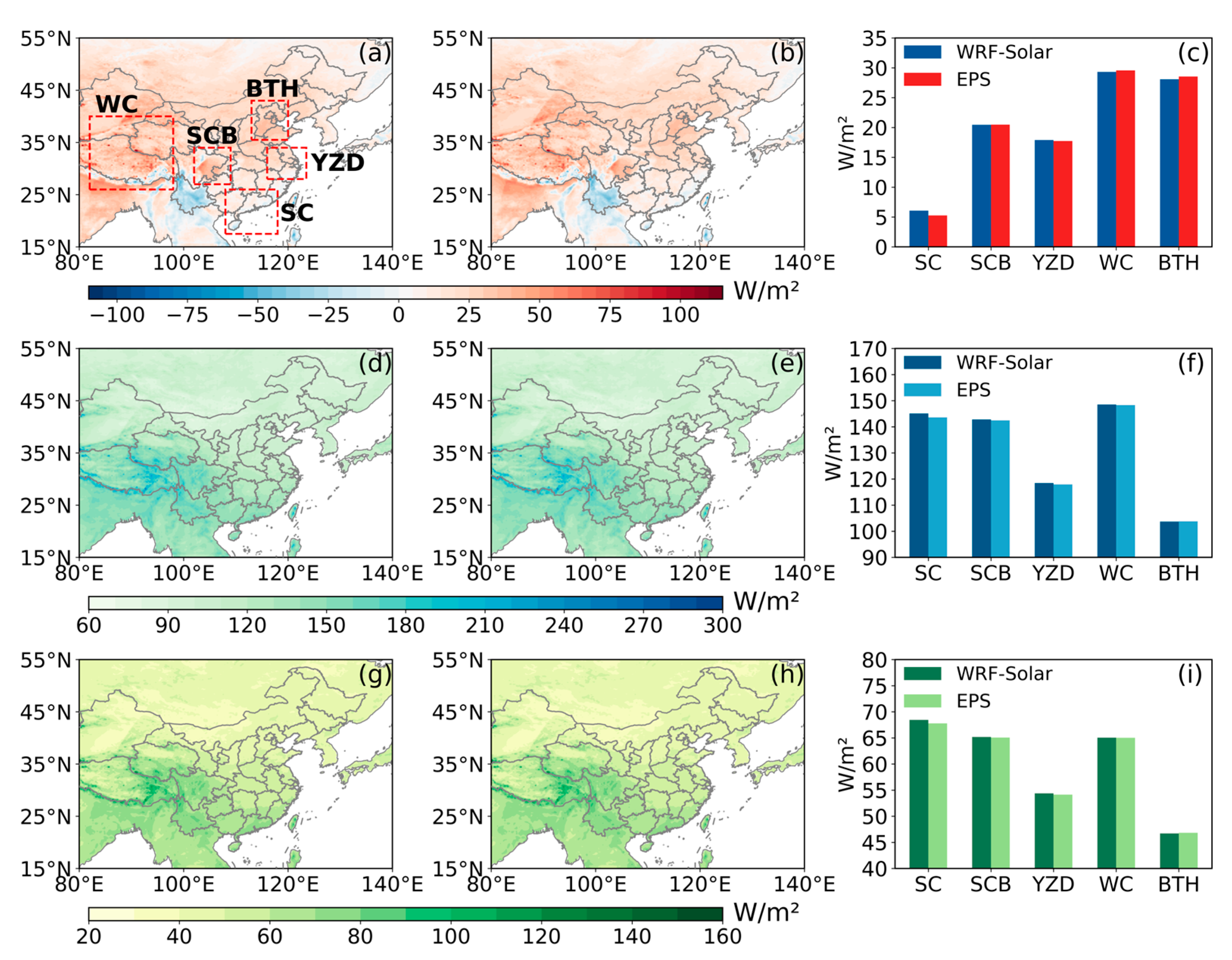
Figure 3a–c present the annual average bias of GHI between WRF-Solar, WRF-Solar EPS estimation, and satellite retrievals. We can see that the estimated annual average GHI is higher than satellite retrieval with the bias of 17.27 W/m2 for WRF-Solar and 17.68 W/m2 for WRF-Solar EPS. Model overestimations were primarily concentrated in northwest China, the North China Plain, the Sichuan Basin, and the northern Indian Peninsula. Specifically, the biases of 5.27 W/m2, 20.47 W/m2, 17.71 W/m2, 29.55 W/m2, and 28.53 W/m2 are obtained, respectively, in the SC, SCB, YZD, WC, and BTH regions for WRF-Solar. At the same time, similar results for WRF-Solar EPS were also observed in these regions (SC: 6.06 W/m2, SCB: 20.45 W/m2, YZD: 17.88 W/m2, WC: 29.30 W/m2, and BTH: 28.08 W/m2). It is noted that model underestimations were observed in the Yunnan–Guizhou Plateau and the Himalayan foothills bordering the Ganges Plain. This widespread overestimation can to some extent be attributed to the inherent limitation of using monthly climatological AOD in the model, which fails to capture the intense and frequent aerosol events in East Asia.
Figure 3d–f present the annual average RMSE of GHI between WRF-Solar, WRF-Solar EPS estimation, and satellite retrievals. The RMSE for WRF-Solar GHI is 116.71 W/m2, which is slightly higher than that of WRF-Solar EPS (116.15 W/m2). High RMSE values concentrate in the plateau and mountainous regions, especially the Himalayas, which indicates that the undulating terrain in these areas may impact the stability of the model performance. Specifically, models show large RMSE values in the SC (WRF-Solar: 145.06 W/m2 and WRF-Solar EPS: 143.62 W/m2), SCB (WRF-Solar: 142.77 W/m2 and WRF-Solar EPS: 142.45 W/m2) and WC (WRF-Solar: 148.49 W/m2 and WRF-Solar EPS: 148.32 W/m2) regions. Low RMSEs were obtained in the YZD (WRF-Solar: 118.44 W/m2 and WRF-Solar EPS: 117.95 W/m2) and BTH (WRF-Solar: 103.71 W/m2 and WRF-Solar EPS: 103.81 W/m2) regions. We have to point out that the SC and BTH regions exhibit distinct characteristics in terms of bias and RMSE among the selected areas. The SC region presents a smaller bias but a larger RMSE, which could be attributed to the differences with high variability and instability in this region. However, the BTH region presents a larger bias but the smallest RMSE, which could be attributed to the stability of model performance but with a systematic shift. According to [43,44], both ground-based and satellite observations have confirmed the high aerosol loading in the North China Plain, where the annual mean AOD often exceeds 0.6. Consequently, an inadequate characterization of the AOD background leads models to underestimate the aerosol radiative effect in the BTH region, thereby causing this systematic bias.
Figure 3g–i present the annual average MAE of GHI between WRF-Solar, WRF-Solar EPS estimation, and satellite retrievals. We can see that the annual average MAE values of GHI for WRF-Solar (51.57 W/m2) and WRF-Solar EPS (51.38 W/m2) are almost the same. Large MAEs were mainly distributed in the southwest of China. Specifically, similar to RMSE, models also show large MAE values in the SC (WRF-Solar: 68.45 W/m2 and WRF-Solar EPS: 67.78 W/m2), SCB (WRF-Solar: 65.18 W/m2 and WRF-Solar EPS: 65.07 W/m2), and WC (WRF-Solar: 65.03 W/m2 and WRF-Solar EPS: 65.01 W/m2) regions. Low RMSEs were obtained in the YZD (WRF-Solar: 54.37 W/m2 and WRF-Solar EPS: 54.13 W/m2) and BTH (WRF-Solar: 46.71 W/m2 and WRF-Solar EPS: 46.83 W/m2) regions. The error in GHI estimation by WRF-Solar in East Asia is comparable to the error result reported by [35] for the contiguous United States, and also aligns well with the model’s performance in studies conducted in other countries or regions [45,46,47].
Among the regions of interest, the ensemble mean forecast demonstrates the most significant improvement in the SC region, with bias reduced by 0.79 W/m2, RMSE reduced by 1.44 W/m2, and MAE reduced by 0.66 W/m2, respectively. Other regions showed minimal improvement, while the BTH region has slight increases with the metrics of bias, RMSE, and MAE. These results indicate that for 36 h forecasts over East Asia, WRF-Solar EPS performs comparably to WRF-Solar.
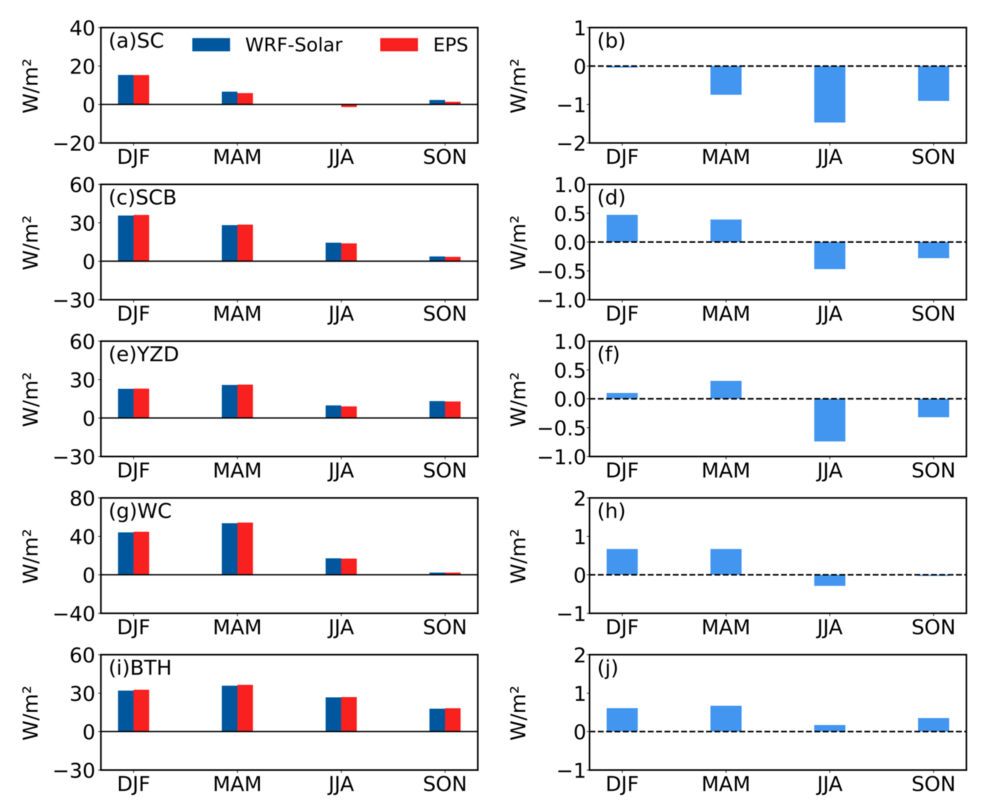
Figure 4 shows the seasonal mean bias of GHI from WRF-Solar and WRF-Solar EPS versus satellite retrievals in the SC, SCB, YZD, WC, and BTH regions from December 2019 to November 2020. Both models have positive bias for each season in almost all regions of interest, with the exception of WRF-Solar EPS, which showed a small negative value (−1.38 W/m2) during JJA in the SC region. At the same time, the biases of the models were generally larger during DJF and MAM compared to JJA and SON. The biases reach their maximum values within a year during DJF in the SC region (WRF-Solar: 15.33 W/m2 and WRF-Solar EPS: 15.29 W/m2) and in the SCB region (WRF-Solar: 35.60 W/m2 and WRF-Solar EPS: 36.07 W/m2), and YZD (WRF-Solar: 25.74 W/m2 and WRF-Solar EPS: 26.05 W/m2), WC (WRF-Solar: 53.58 W/m2 and WRF-Solar EPS: 54.25 W/m2), BTH (WRF-Solar: 35.77 W/m2 and WRF-Solar EPS: 36.44 W/m2) have their own maximum values during the MAM period.
The ensemble mean forecast has different effects on different regions across the seasons, with the WRF-Solar EPS showing no significant reduction in bias during DJF and MAM in most regions. However, during JJA and SON, it demonstrates a certain level of improvement in reducing bias. Notably, the WRF-Solar EPS has the most pronounced effect in reducing the overestimation in the SC region, where its bias is consistently lower than that of WRF-Solar. The maximum bias difference between WRF-Solar EPS and WRF-Solar in the SC region is observed during JJA, reaching −1.47 W/m2. Moreover, the bias of WRF-Solar EPS across all seasons in the BTH region is greater than that of WRF-Solar, indicating that the ensemble mean forecast does not significantly enhance the GHI prediction in bias for this area.
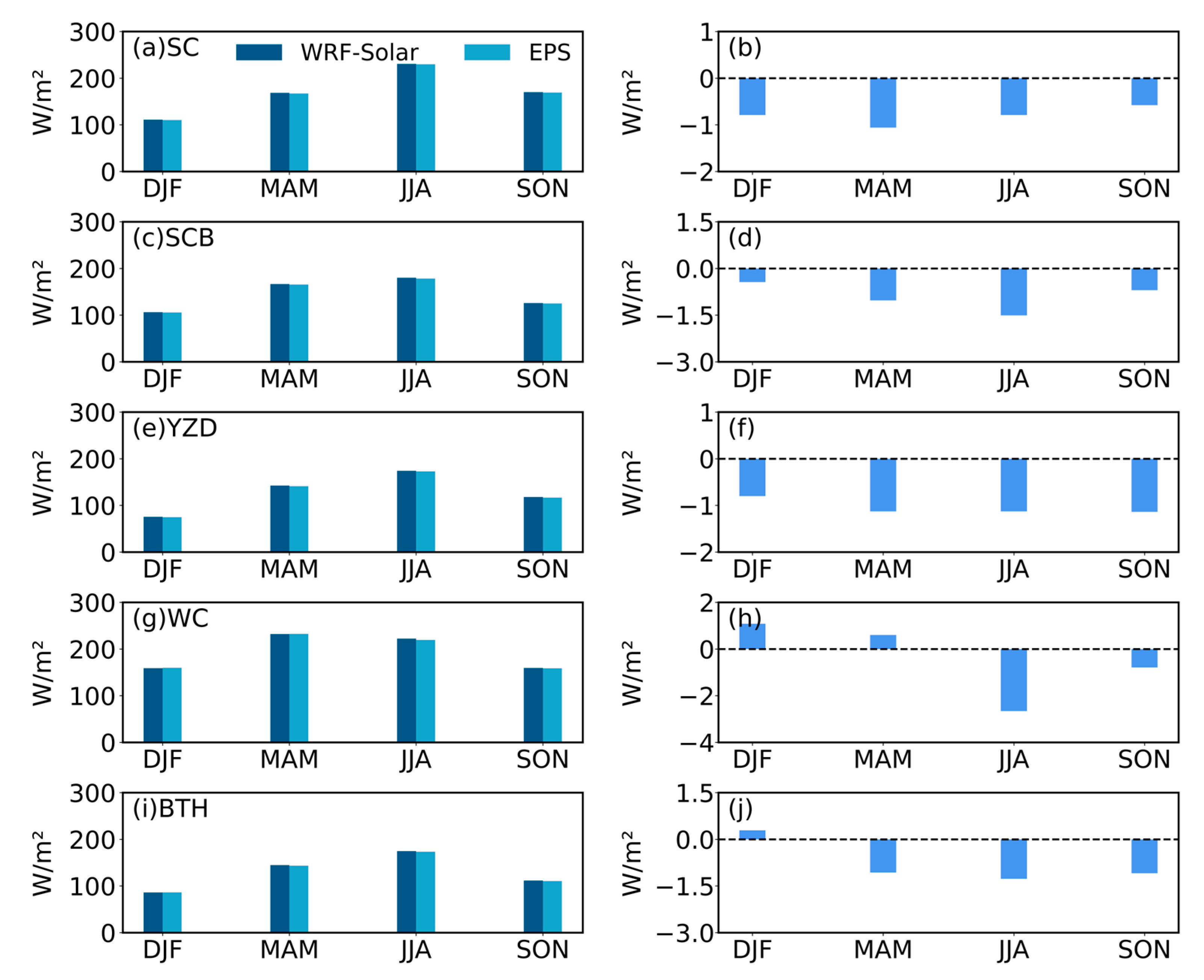
Figure 5 illustrates the comparison of seasonal average RMSE of GHI from WRF-Solar and WRF-Solar EPS versus satellite retrievals across the regions of interest. In all the regions of interest, both models exhibit smaller RMSE during the DJF period, with WRF-Solar showing RMSE values of 116.00 W/m2, 113.27 W/m2, 87.31 W/m2, 106.17 W/m2, and 79.95 W/m2 for SC, SCB, YZD, WC, and BTH, respectively. The corresponding results for WRF-Solar EPS were 115.43 W/m2, 113.60 W/m2, 87.16 W/m2, 106.80 W/m2, and 80.71 W/m2. The sole exception is the BTH region, where the minimum RMSE occurs during the SON period, with values of 77.40 W/m2 and 77.19 W/m2 for WRF-Solar and WRF-Solar EPS, respectively. The maximum RMSE is observed during the JJA period, and the RMSE values of WRF-Solar in SC, SCB, YZD, WC, and BTH were 160.7 W/m2, 166.38 W/m2, 148.66 W/m2, 176.52 W/m2, and 136.55 W/m2, respectively. The values of WRF-Solar EPS were 157.80 W/m2, 165.35 W/m2, 147.76 W/m2, 175.32 W/m2, and 136.55 W/m2, respectively. WRF-Solar EPS has a small improvement in RMSE in each region during JJA and SON, among which the improvement effect is the largest in SC area, and the difference in RMSE between WRF-Solar EPS and WRF-Solar in SC area is −2.9 W/m2, while the the RMSE in BTH region decreased by only 0.37 W/m2 and 0.21 W/m2 during JJA and SON, respectively.
In summary, the errors in GHI estimation by the models exhibit the characteristic of increasing with the solar irradiance. It is noteworthy that there is a temporal mismatch in the periods when the bias and RMSE of the model’s GHI estimation reach their maximum values. The maximum bias typically occurs during the winter and spring seasons, whereas the maximum RMSE occurs in the summer. The possible reason for this phenomenon is related to the different sources of error dominated by the model in different seasons. The primary factors contributing to the peak RMSE during summer may be insufficient cloud simulation. This period is characterized by intense East Asian summer monsoon activity, marked by intense convection, high humidity, and complex cloud life cycles [48]. As demonstrated by [49], cloud microphysics parameterization is a major source of uncertainty in solar radiation forecasting under cloudy conditions. The complex dynamical cloud environment during summer leads to larger forecast errors, resulting in high RMSE. Conversely, the maximum bias in winter and spring points towards a more systematic error source. The inaccurate characterization of AOD by the models is a major part, leading to a persistent and systematic overestimation of GHI.
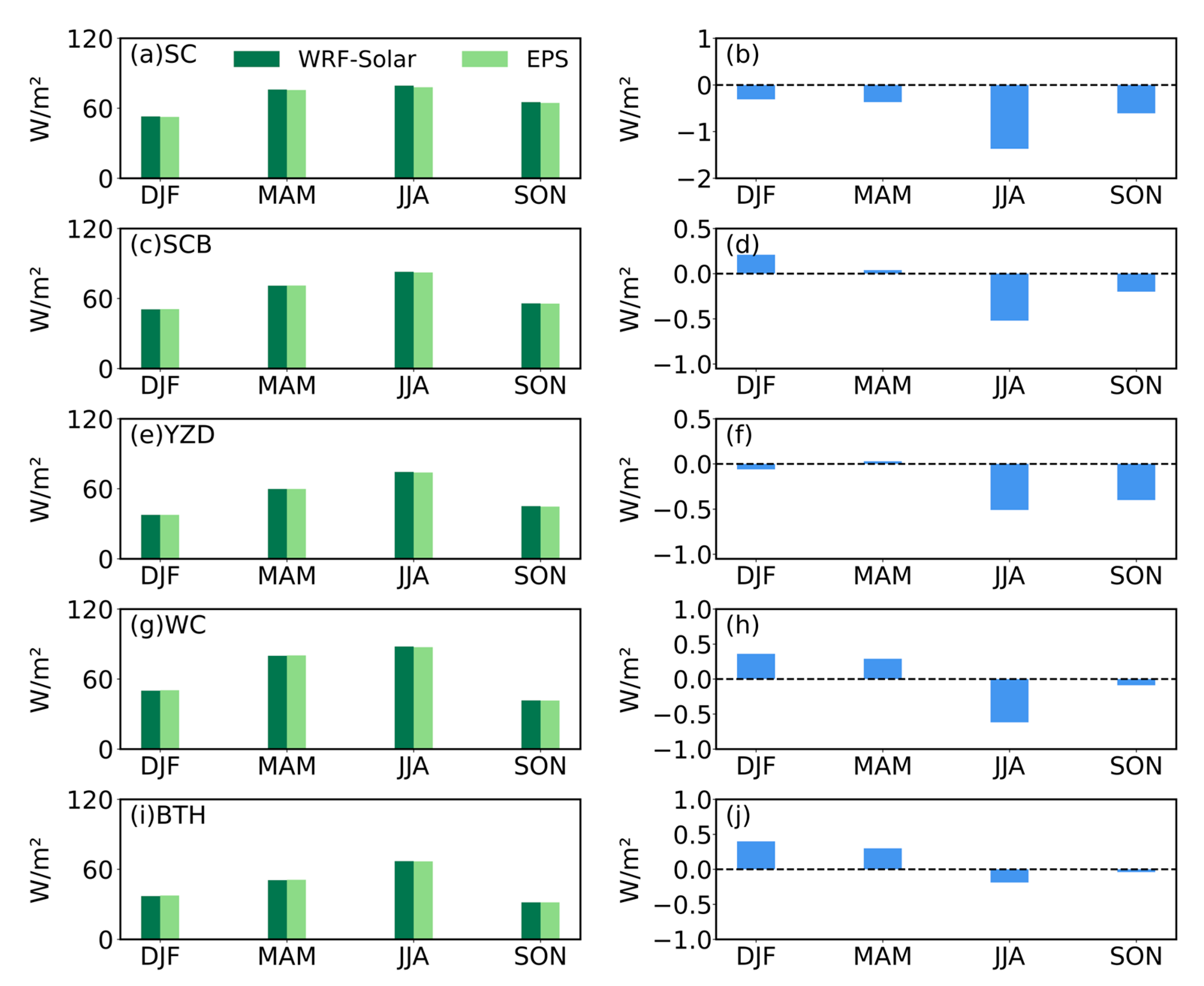
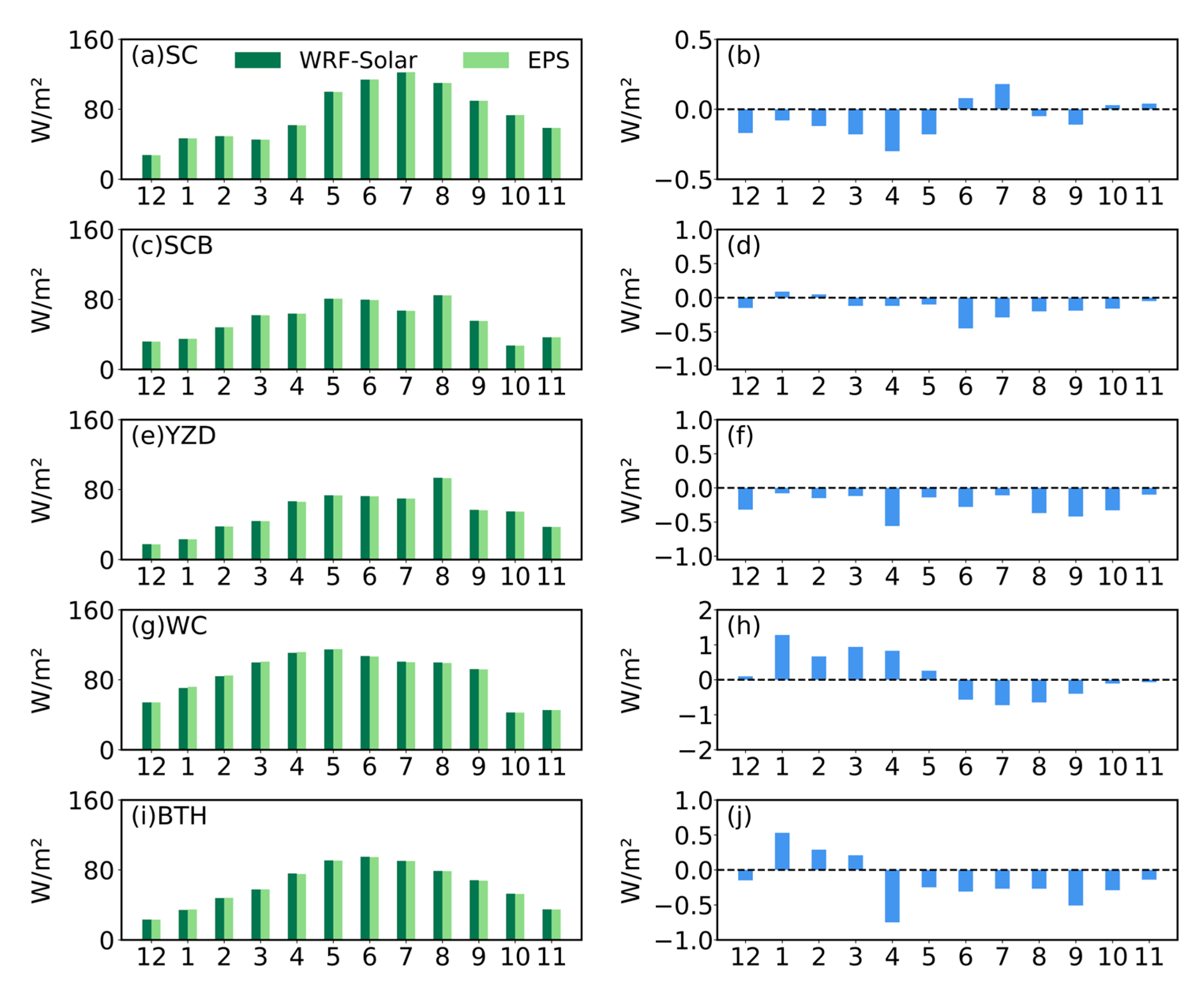
The comparison of the seasonal mean MAE of GHI from WRF-Solar and WRF-Solar EPS versus satellite retrievals in the selected areas is shown in Figure 6. The overall characteristics of MAE were similar to those of RMSE, with the SC, SCB, and YZD regions having the smallest MAE during DJF; the MAE for WRF-Solar in these areas were 52.92 W/m2, 50.70 W/m2, and 37.69 W/m2, respectively, and the MAE of WRF-Solar EPS were 52.61 W/m2, 50.91 W/m2, and 37.63 W/m2. The WC and BTH have the smallest MAE during SON, with WRF-Solar and WRF-Solar EPS values of 41.59 W/m2 and 31.70 W/m2 and 41.68 W/m2 and 31.66 W/m2, respectively. During the JJA, the MAE reaches its maximum values in all regions. The RMSE values of WRF-Solar in the SC, SCB, YZD, WC, and BTH regions were 79.38 W/m2, 82.88 W/m2, 74.46 W/m2, 87.95 W/m2, and 67.04 W/m2, respectively. The values for WRF-Solar EPS were 78.01 W/m2, 82.36 W/m2, 73.95 W/m2, 87.33 W/m2, and 66.85 W/m2, respectively. The improvement in MAE by WRF-Solar EPS is most significant in SC region, where during the JJA period, the maximum reduction in MAE reaches 1.37 W/m2. This indicates that the improvement of the model’s short-term capability to predict GHI through ensemble averaging is relatively minor during the winter and spring, while the enhancement is more pronounced in summer and autumn.
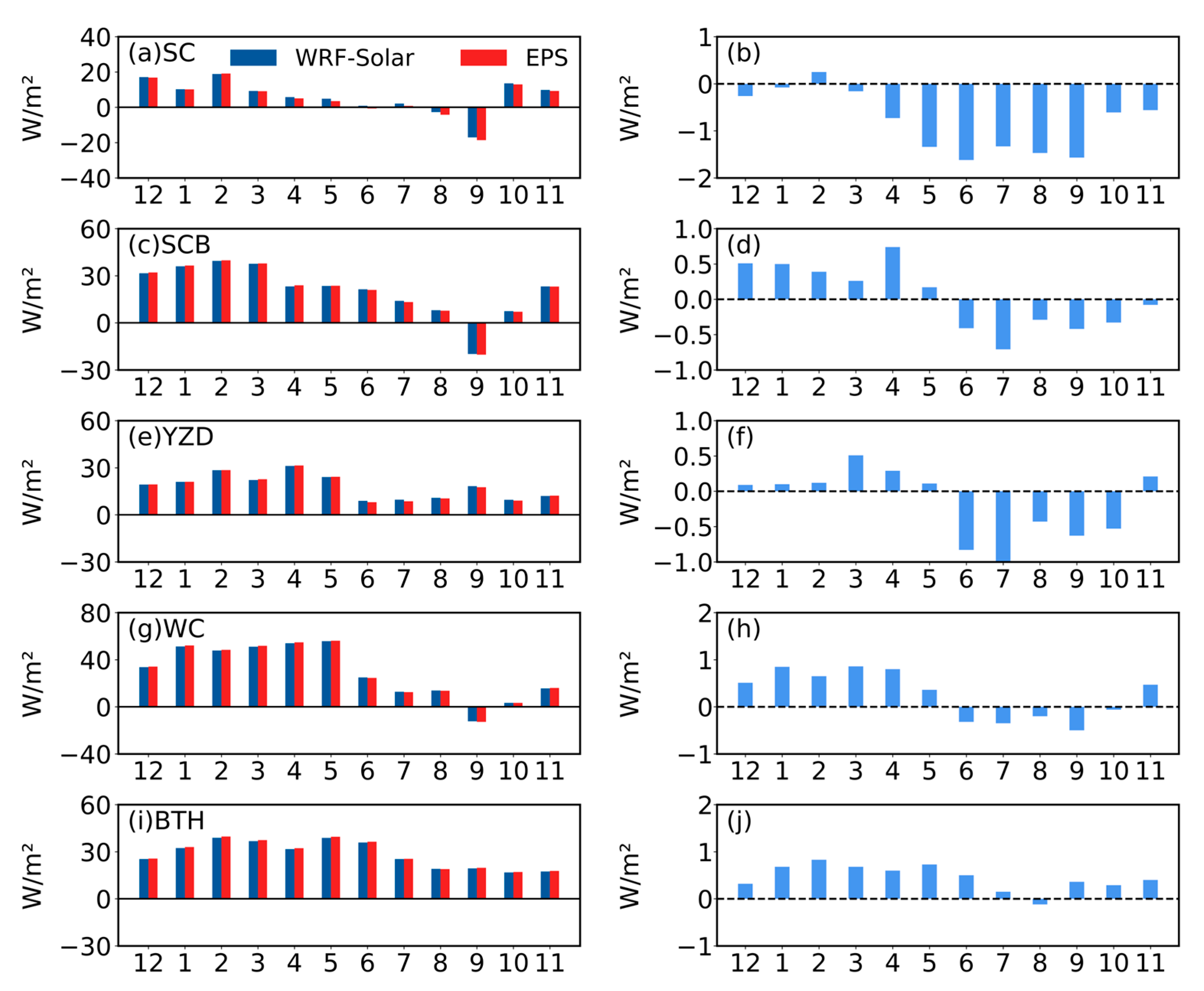
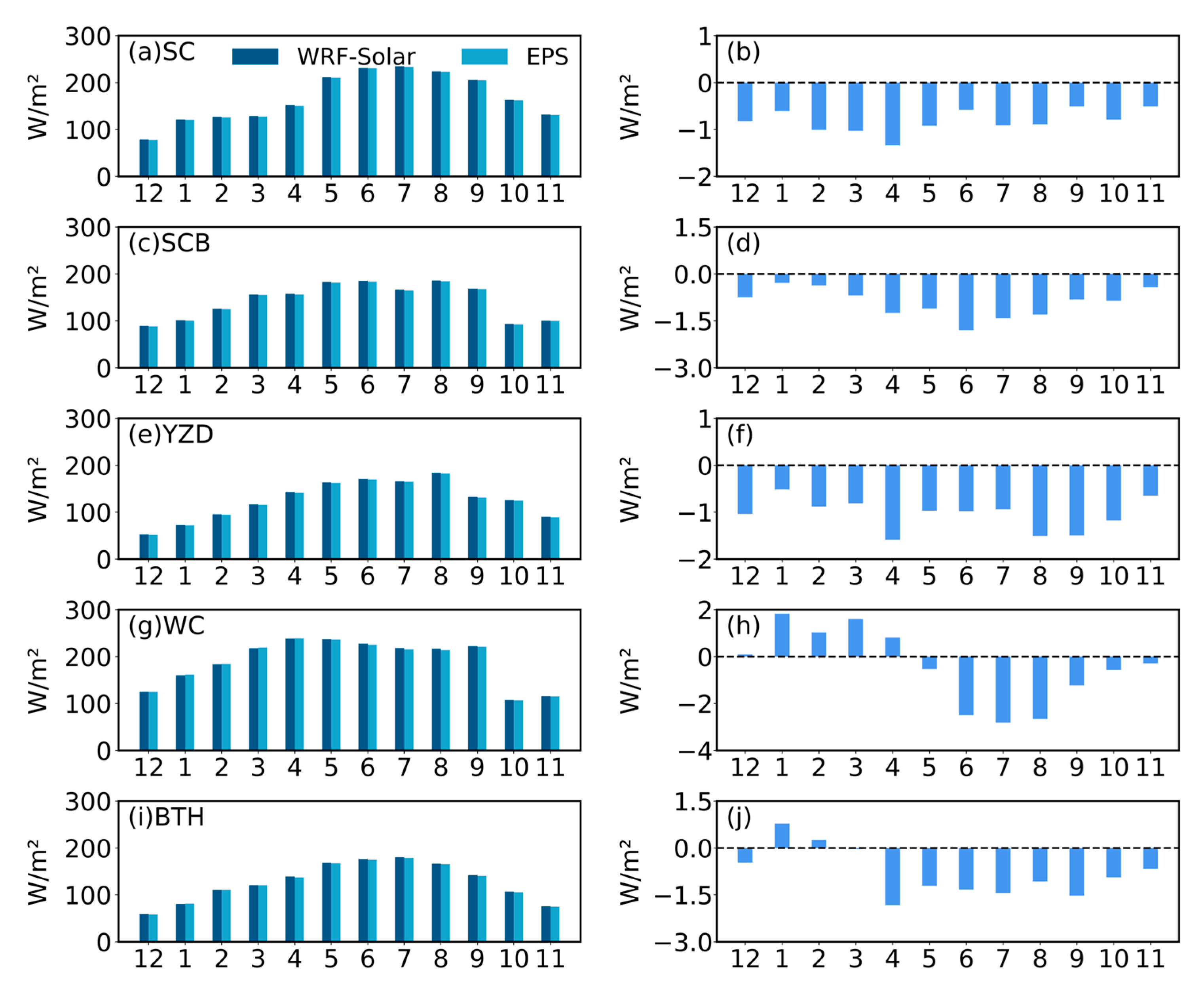
Figure 7 presents the monthly mean bias comparisons of GHI between model simulations (WRF-Solar and WRF-Solar EPS) and satellite retrievals from December 2019 to November 2020 in the regions of interest. It is noted that regional biases in GHI have pronounced fluctuations: larger discrepancies occur from December to June, while biases remain relatively smaller from July to November. Among the regions, WC region showed the most significant bias, peaking at 55.77 W/m2 of WRF-Solar and 56.13 of WRF-Solar EPS in May. Positive biases were observed in all regions throughout the year, except for BTH and WC regions in September and the SC region in August and September.
The difference between WRF-Solar EPS and WRF-Solar bias also exhibits temporal fluctuations. During the period from December to May, the ensemble mean bias is generally greater than WRF-Solar across most regions (SCB, YZD, and WC). Conversely, from June to November, the bias is smaller than that of WRF-Solar. Notably, WRF-Solar EPS showed the most significant reduction in bias for the SC region, with the bias being lower than WRF-Solar in almost all months. The maximum reduction in bias, reaching 1.62 W/m2, occurs in June. In the BTH region, the ensemble mean does not show a significant improvement in bias.
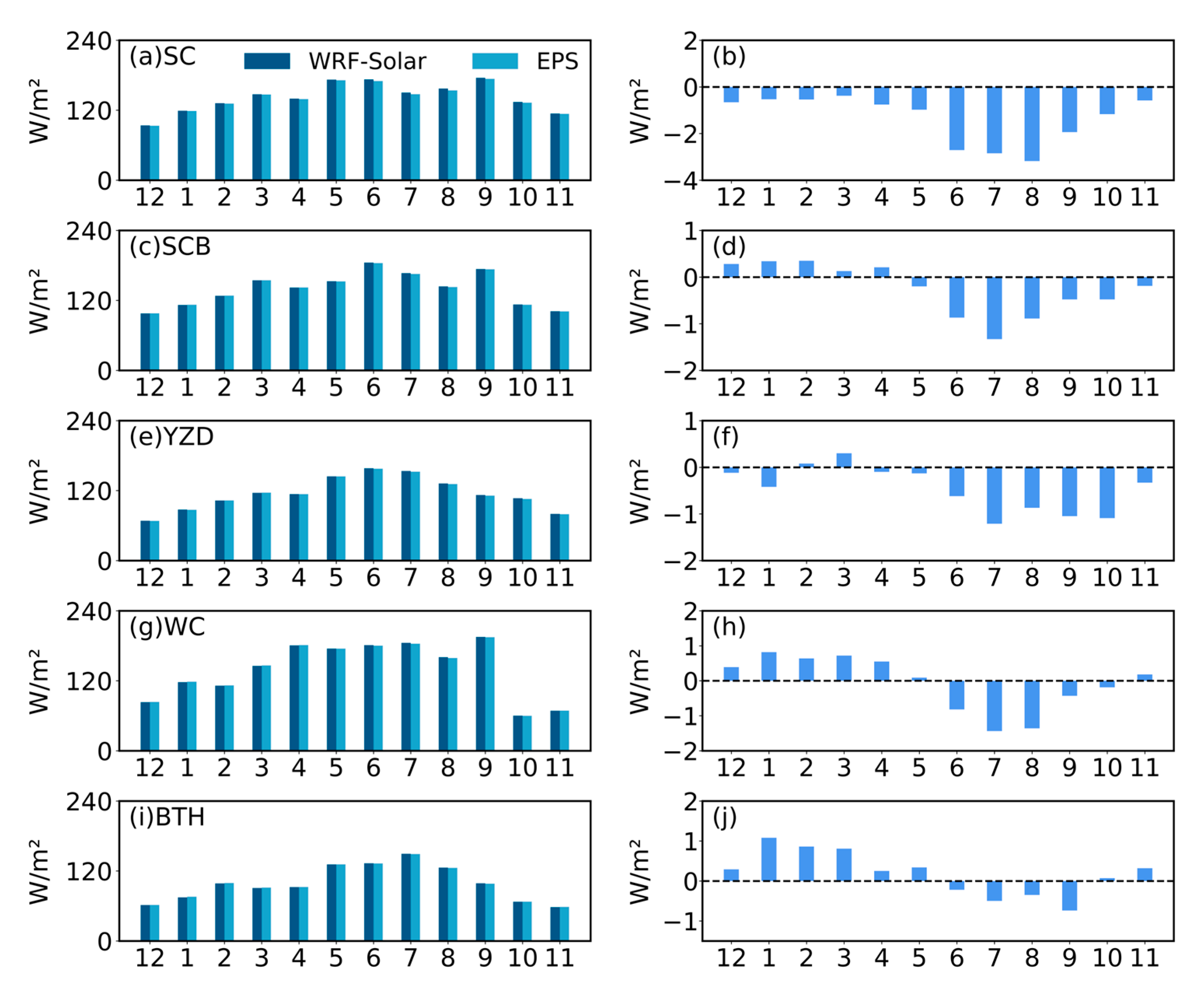
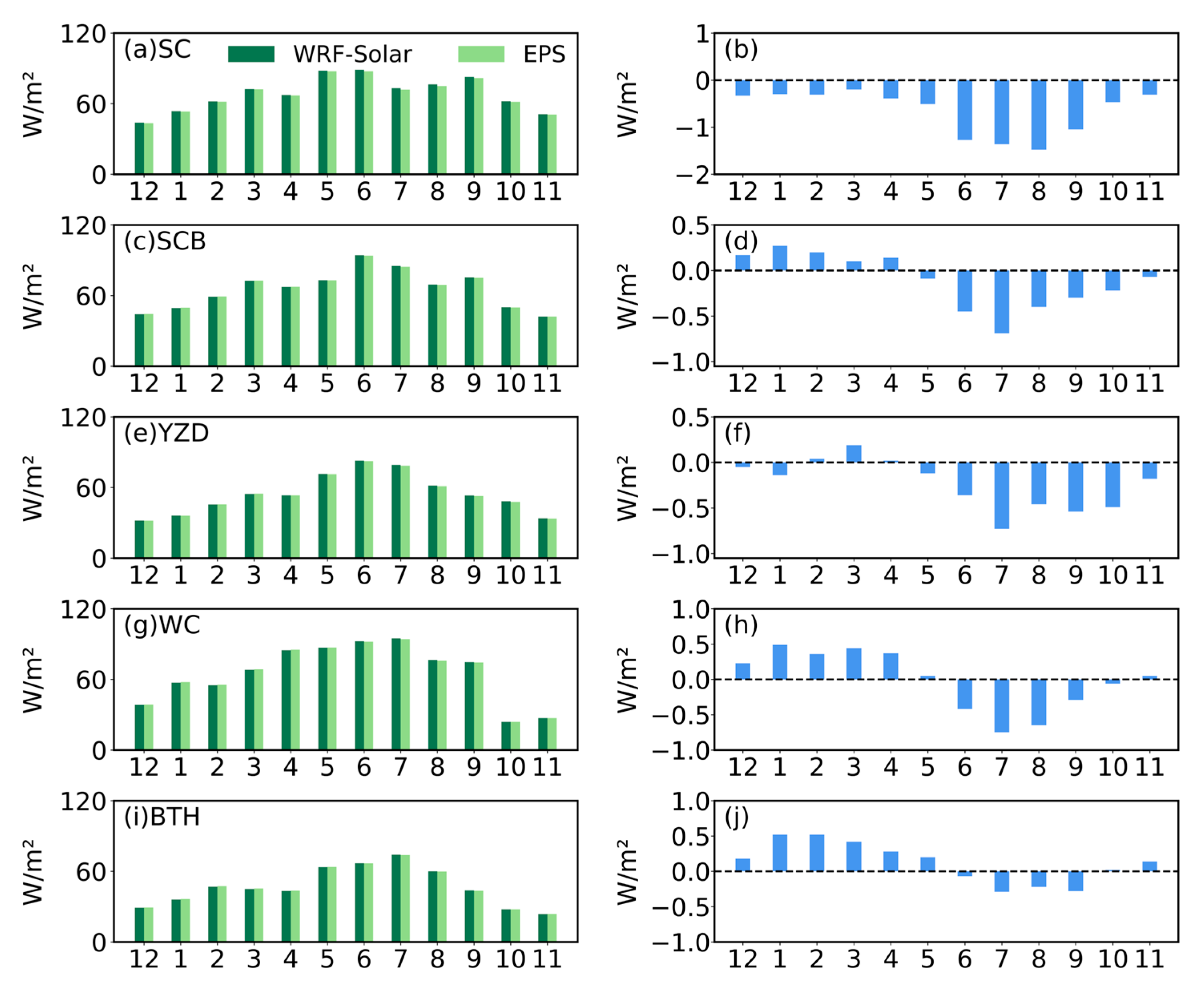
The RMSE and MAE further reveal that large differences were obtained in June and July over all regions (Figure 8 and Figure 9). It is worth noting that in response to the negative bias observed in the SC, SCB, and WC regions during September, the RMSE for these three regions also exhibits notably high values in that month, RMSE of WRF-Solar in these three regions were 175.71 W/m2, 173.84 W/m2, and 195.23 W/m2, and the results of WRF-Solar EPS were 173.77 W/m2, 173.84 W/m2, and 195.23 W/m2, respectively. During the period from December to May, for WC, SBC, and BTH, the RMSE and MAE of WRF-Solar EPS increase slightly compared to WRF-Solar, while for YZD and SC, there is a slight decrease. Between June and November, the RMSE and MAE for almost all regions show varying degrees of reduction compared to WRF-Solar, with the largest reduction generally occurring between July and August. Among these regions, SC exhibits the most significant reduction, with its RMSE and MAE decreasing by a maximum of 3.18 W/m2 and 1.48 W/m2 in August, respectively.

3.2. Assessment of WRF-Solar and EPS DIR Estimation

Figure 10 displays the annual average DIR from December 2019 to November 2020, generated by WRF-Solar, WRF-Solar EPS, and satellite retrievals. Unlike GHI, DIR exhibits higher sensitivity to feedback processes of aerosol and cloud [49,50,51]. Consequently, inaccuracies in simulating these components constitute the primary source of error in DIR modeling. WRF-Solar and WRF-Solar EPS show similar radiation distribution characteristics to the satellite results, with high DIR values primarily found in the western Tibetan Plateau of China, Inner Mongolia, Mongolia, and the Indo-China Peninsula. Low values were observed in the southern Tibetan Plateau, Sichuan Basin region, and high-latitude areas. Both models exhibit systematic underestimation compared to satellite retrievals. WRF-Solar EPS slightly exceeds WRF-Solar in average radiation. The regional mean DIR derived from WRF-Solar, WRF-Solar EPS, and satellite retrievals is 98.89 W/m2, 100.33 W/m2, and 110.26 W/m2, respectively.
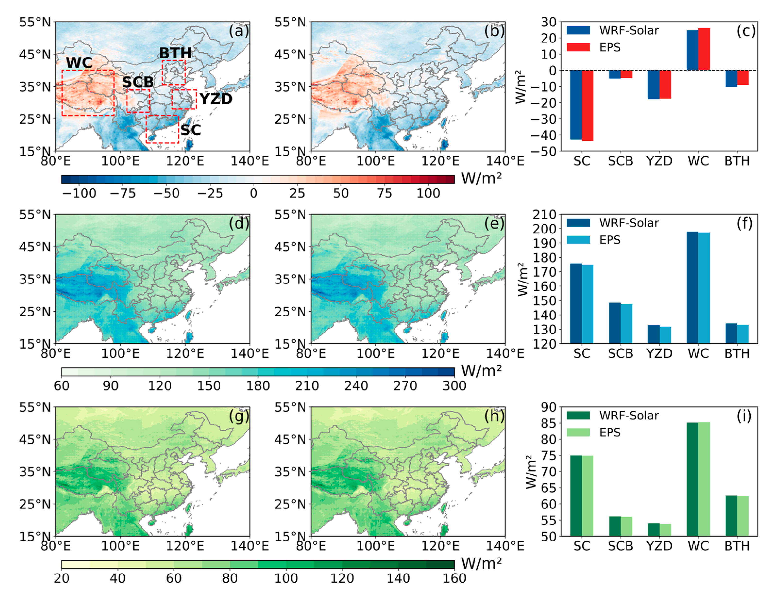
Figure 11a–c show the annual average bias of DIR between WRF-Solar, WRF-Solar EPS estimation, and satellite retrievals. The DIR estimated by WRF-Solar was 11.37 W/m2 lower than the satellite observations, while the results from the WRF-Solar EPS were 9.93 W/m2 below the satellite observations. Unlike the systematic overestimation in GHI (Figure 3a–c), DIR from both models exhibits regionally opposing biases, positive bias dominates the Tibetan Plateau, Qinghai, Gansu, and certain parts of the Gangetic Plain, and negative bias prevails in southern China and Indo-China Peninsula. The biases of −42.85 W/m2, −5.24 W/m2, −17.80 W/m2, 24.60 W/m2, and −10.36 W/m2 were, respectively, obtained in the SC, SCB, YZD, WC, and BTH regions for WRF-Solar. Concurrently, results from WRF-Solar EPS in these regions were values of −43.69 W/m2 in SC, −4.91 W/m2 in SCB, −17.63 W/m2 in YZD, 26.06 W/m2 in WC, and −9.15 W/m2 in BTH. The results of the two models exhibit similarity. Among all the regions of interest, WC is the only area that showed a positive bias. The primary reason for this situation is the significant underestimation of cloud by the CLD3 sub-grid scale cloud scheme employed in the models, particularly over the Tibetan Plateau, leading to an overestimation of DIR.
Figure 11d–f present the annual average RMSE of direct shortwave radiation between WRF-Solar and WRF-Solar EPS estimates versus satellite retrievals. Compared to the RMSE for GHI, significantly higher RMSE values were observed for DIR estimates from both WRF-Solar and WRF-Solar EPS. The RMSE for WRF-Solar is 150.12 W/m2, while the result for WRF-Solar EPS is 148.99 W/m2. Regions with relatively higher RMSE were predominantly concentrated over the Tibetan Plateau. Among the regions of interest, both models exhibit higher RMSE values in the SC (WRF-Solar: 175.75 W/m2 and WRF-Solar EPS: 174.91 W/m2) and WC regions (WRF-Solar: 197.82 W/m2 and WRF-Solar EPS: 197.33 W/m2). Relatively lower RMSE were obtained in the SCB (WRF-Solar: 148.42 W/m2 and WRF-Solar EPS: 147.45 W/m2), YZD (WRF-Solar: 132.89 W/m2 and WRF-Solar EPS: 131.84 W/m2), and BTH (WRF-Solar: 134.00 W/m2 and WRF-Solar EPS: 133.13 W/m2) regions
The MAE of DIR between WRF-Solar and WRF-Solar EPS estimation, which shares similar characteristics with RMSE, is presented in Figure 11g–i. The average MAE of WRF-Solar in SC, SCB, YZD, WC, and BTH is 74.99 W/m2, 56.11 W/m2, 54.07 W/m2, 85.14 W/m2, and 62.57 W/m2, and the MAE of WRF-Solar EPS is 74.92 W/m2, 55.97 W/m2, 53.82 W/m2, 85.27 W/m2, and 62.40 W/m2, respectively.
Compared to the results of GHI, although the mean DIR is generally lower than GHI, WRF-Solar and WRF-Solar EPS exhibit higher RMSE and MAE, indicating greater uncertainty in the model’s prediction of DIR. Both WRF-Solar and WRF-Solar EPS exhibit large errors in the SC and WC region, which may be due to the inaccurate simulation of the dissipation process of the low and medium clouds by models in these areas [50,51]. The WRF-Solar EPS showed a very slight improvement in the simulation of DIR, with RMSE and MAE decreasing by 1.23 and 0.22 W/m2, respectively. The RMAE and MAE for the selected five regions also exhibit minor reductions. Among the regions, the YZD region demonstrated the most effective improvement, with a bias reduction of 0.17 W/m2, and decreases in RMSE and MAE to 1.04 W/m2 and 0.25 W/m2, respectively. This also indicates that the 36 h forecasting capabilities of WRF-Solar EPS and WRF-Solar for DIR in East Asia are on par.
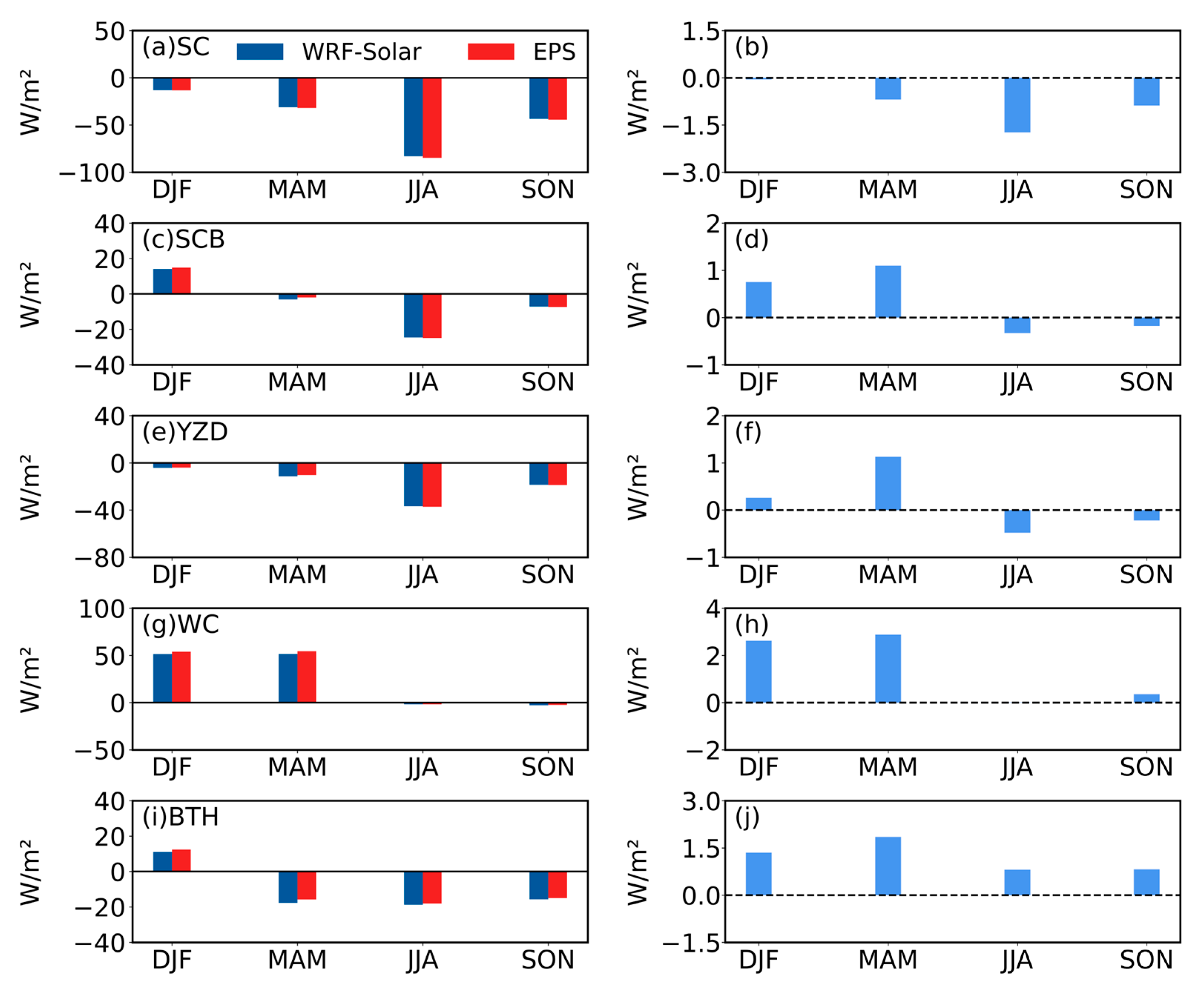
Figure 12 depicts the comparison of seasonal average DIR biases between WRF-Solar and WRF-Solar EPS against satellite retrievals for the regions SC, SCB, YZD, WC, and BTH. In the regions of interest, WRF-Solar and WRF-Solar EPS exhibit a consistent bias tendency across all seasons, with negative bias observed over a majority of seasons. During JJA and SON, the biases were negative across all regions, with SC showing the largest negative bias among the regions of interest in JJA, with WRF-Solar and WRF-Solar EPS reporting biases of −83.12 W/m2 and −84.86 W/m2, respectively. During DJF, SCB, and BTH regions exhibit a minor positive bias, while WC showed a significantly higher positive bias during both DJF and MAM. Significant negative DIR biases in the SC and YZD regions, particularly during summer, may be related to the simulation of cloud properties by the microphysics scheme. The model tends to overestimate cloud fraction during summer, when convective activities are extensive, consistent with findings by [35,49]. Furthermore, Ref. [49] pointed out that excessive spurious high clouds generated by the model reduce DIR while simultaneously overestimating diffuse radiation. Under such compensatory effects, the model’s simulation error for GHI is reduced, which aligns with our previous evaluation results for GHI. Specifically, during DJF, the biases for WRF-Solar and WRF-Solar EPS were 51.39 W/m2 and 54.01 W/m2, respectively, and during MAM, they were 51.60 W/m2 and 54.48 W/m2, respectively. The performance of DIR estimation by WRF-Solar EPS in terms of bias does not show a significant improvement compared to WRF-Solar. Across the four seasons, WRF-Solar EPS exacerbates the underestimation observed in the SC region. The ensemble mean forecast also exhibits a more pronounced increase in bias for the WC region during DJF and MAM. The BTH region is the only area where WRF-Solar EPS demonstrates a relatively stable improvement, with bias reductions in MAM, JJA, and SON periods. Specifically, during MAM, WRF-Solar EPS improved the bias by 1.85 W/m2 compared to WRF-Solar.
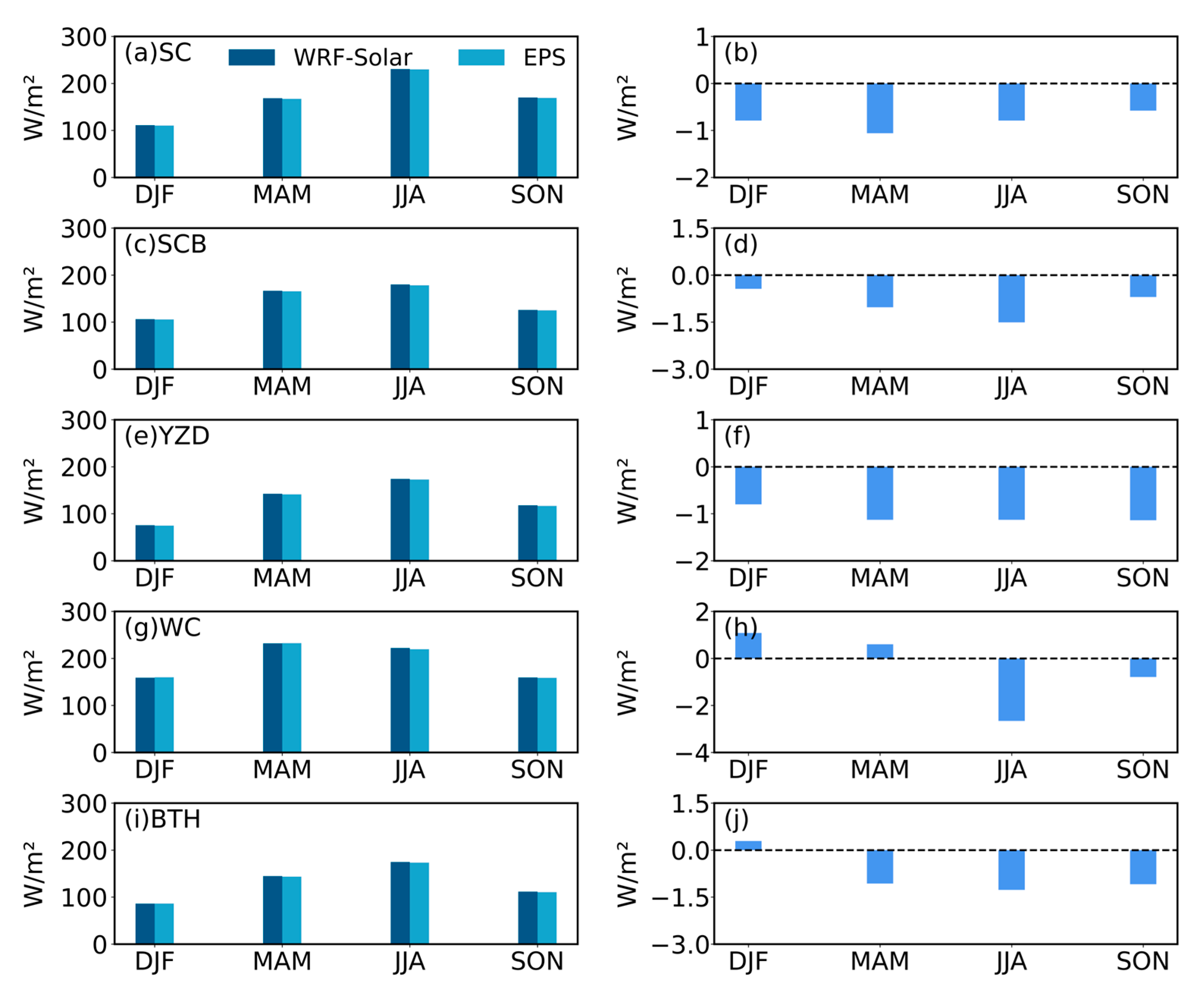
The seasonal average RMSE and MAE of DIR for all regions of interest are depicted in Figure 13 and Figure 14. The RMSE fluctuations across four seasons exhibit two distinct patterns. In regions of SC, SCB, YZD, and BTH, the RMSE reaches its peak during JJA, with WRF-Solar showing RMSE of 230.64 W/m2, 179.90 W/m2, 174.14 W/m2, and 174.68 W/m2, respectively. The RMSE of WRF-Solar EPS in the aforementioned regions was 229.85 W/m2, 178.39 W/m2, 173.01 W/m2, and 173.41 W/m2, respectively. In the WC region, the RMSE reaches its maximum during the MAM, with WRF-Solar yielding a value of 232.02 W/m2 and WRF-Solar EPS a value of 232.62 W/m2. The improvement of WRF-Solar EPS in terms of RMSE is relatively stable, and the RMSE showed a decrease for SC, SCB, YZD, and during MAM, JJA, and SON of BTH. There is no improvement in RMSE during DJF and MAM for WC region, but there is a significant decrease in RMSE during JJA and SON, and the difference between RMSE and WRF-Solar during JJA is the largest, which is −2.66 W/m2.
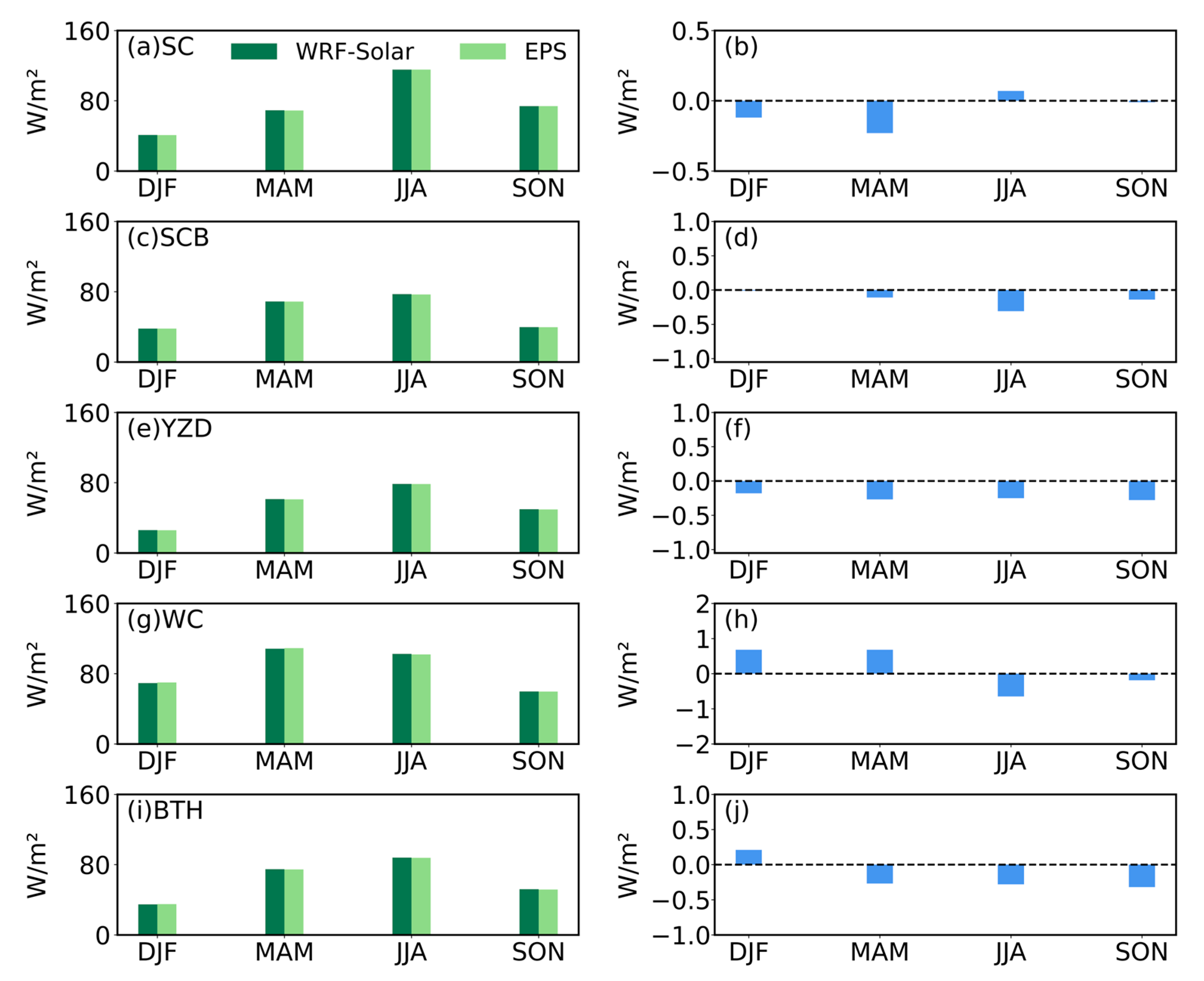
The seasonal mean characteristics of MAE for the model-estimated DIR are similar to those of the RMSE, with the maximum MAE of SC, SCB, YZD, and BTH during JJA being 115.45 W/m2, 77.24 W/m2, 78.66 W/m2, and 88.08 W/m2 for WRF-Solar, and 115.52 W/m2, 79.63 W/m2, 78.41 W/m2, and 87.8 W/m2 for WRF-Solar EPS. The maximum MAE is 108.43 W/m2 in WC region and 109.11 W/m2 in WRF-Solar EPS during MAN. The average MAE of WRF-Solar EPS shows a relatively stable decrease in SC, SCB, YZD, and BTH during most seasons. During the JJA, the difference in MAE between WRF-Solar EPS and WRF-Solar is the largest, which is −0.65 W/m2.
The above results indicate that the errors in the model’s forecasts of DIR for the WC region exhibit specific characteristics. Ensemble mean forecast contributes to enhancing the stability of the model’s forecasts of DIR to a limited extent.
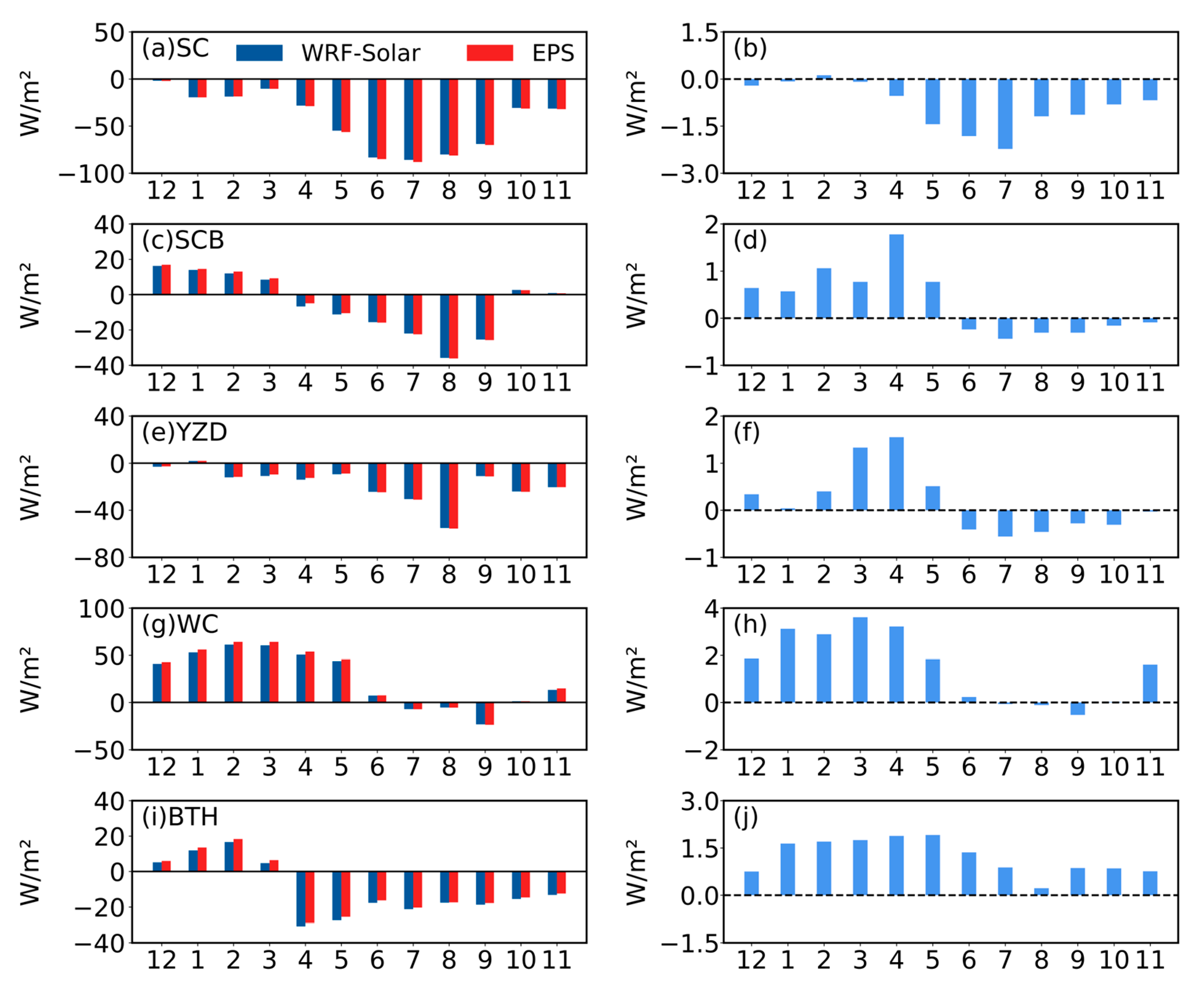
Figure 15 illustrates the monthly mean DIR bias between WRF-Solar/WRF-Solar EPS model outputs and satellite retrievals across the regions of interest for December 2019 to November 2020. The average bias of different months showed very distinct characteristics from the comparison results of GHI. The bias in the WC and SC regions exhibits significant volatility. From January to May, the WC showed a large positive bias pattern, and its maximum value at 61.24 W/m2 of WRF-Solar and 64.13 W/m2 of WRF-Solar EPS in February. After June, the amplitude of bias in the WC decreases significantly. At the same time, from May to September, the negative bias of the SC began to increase, and it reaches the largest negative bias in June, which is −85.91 W/m2 of WRF-Solar and −88.14 W/m2 of WRF-Solar EPS. The difference between the monthly mean bias of WRF-Solar EPS and WRF-Solar showed that WRF-Solar EPS mainly tends to increase the amplitude of bias, and it can be seen that the ensemble forecast aggravates the overestimation of DIR in the WC, BTH, and SCB from December to May and the underestimation of SC and YZD from May to November. Only in the May to November period is there a certain improvement in the average bias for BTH.
The comparison results between RMSE and MAE with similar characteristics are, respectively, presented in Figure 16 and Figure 17. Except for WC, where the maximum RMSE and MAE values occur in April and May, respectively (with maximum RMSE and MAE values of 238.14 W/m2 and 114.73 W/m2), the RMSE and MAE values in other regions increase over time and reach their peak in June. Among these, SC exhibits the highest RMSE and MAE, with values of 234.52 W/m2 and 122.22 W/m2, respectively. Regarding the comparison between RMSE and MAE, except for the period between December and May, the WRF-Solar EPS has led to a small increase in RMSE and MAE for WC, BTH, and SBC. The ensemble mean has brought about a certain degree of improvement in RMSE and MAE, with the improvement being more significant in most regions between April and September. The improvement in WC is larger, with RMSE and MAE reduced by a maximum of 2.82 W/m2 and 0.73 W/m2, respectively.

4. Discussion

WRF-Solar and WRF-Solar EPS effectively reproduce the large-scale spatial distribution characteristics of solar radiation over East Asia, although regional and seasonal errors still exist. The systematic overestimation by GHI and the peak bias pattern observed during winter and spring are largely attributable to the inadequate representation of actual aerosol loading by the monthly climatological aerosol optical depth (AOD) data used in the model, particularly during the polluted winter and spring seasons. The peak in RMSE/MAE observed during summer suggests that the dominant error sources may vary seasonally, the high variability of cloud cover during the summer monsoon season and its inaccurate simulation may be key factors contributing to increased errors during this period. The distinct overestimation of DIR in the WC region may be related to the inadequate cloud representation of some regions (e.g., the complex terrain region of southwest China) by the CLD3 scheme in the current model configuration [51]. These results are consistent with previous studies indicating that aerosols and clouds remain the primary sources of uncertainty in WRF-Solar radiation forecasts [15,16]. Moreover, the insufficient representation of aerosol–cloud feedback in microphysical schemes may further increase uncertainty by affecting cloud property parameters such as cloud droplet number concentration and effective radius [51,52].
Regarding the short-term (≤36 h) WRF-Solar EPS forecasts, the results indicate that, while ensemble averaging improves stability (RMSE/MAE), it fails to correct systematic biases. This limitation is likely twofold: first, the forecast window is too short for initial perturbations to fully propagate and generate significant ensemble spread; second, perturbing a static and already underestimated climatological AOD field cannot correct the fundamental systematic errors originating from the input data.
Therefore, improving solar irradiance forecasting of WRF-Solar in East Asia can be improved by enhancing the simulation of aerosol–cloud–radiation feedback by utilizing high-resolution AOD retrieval data from geostationary satellites, such as Himawari-8/9 or Fengyun-4 [53,54,55], combined with advanced microphysics schemes (e.g., the Thompson aerosol-aware scheme), and improving the representation of clouds in complex terrain.

5. Conclusions

This study quantitatively evaluated the short-term (≤36 h) predictive performance of WRF-Solar and WRF-Solar EPS for GHI and DIR over East Asia (December 2019–November 2020) by comparing simulations with satellite retrievals. Key findings are summarized as follows:
(1)
WRF-Solar and WRF-Solar EPS effectively captured the spatial patterns of surface GHI over East Asia, with high radiation areas concentrated in the Qinghai–Tibet Plateau and Indo-China Peninsula, and low radiation areas in northern East Asia and the Sichuan Basin. However, both models exhibited a systematic overestimation of GHI compared to satellite retrievals over East Asia (annual mean biases: 17.27 W/m2for WRF-Solar and 17.68 W/m2for WRF-Solar EPS). Overestimations were most pronounced in northwest China, the North China Plain, the Sichuan Basin, and the northern Indian Peninsula. It is noted that the temporal patterns of bias and other error metrics (RMSE and MAE) diverged: maximum biases occurred in winter (DJF) and spring (MAM), whereas peak RMSE/MAE appeared in summer (JJA).
(2)
DIR exhibited larger regional disparities in model performance. Unlike GHI, DIR simulations showed contrasting biases: positive biases dominated the Tibetan Plateau, Qinghai, Gansu, and parts of the Gangetic Plain, while negative biases prevailed in southern China and the Indo-China Peninsula. Specifically, the WC was uniquely characterized by persistent overestimation, whereas the SC, SCB, YZD, and BTH exhibited significant underestimations. Both models yielded higher RMSE and MAE for DIR than for GHI, with peak errors in the SC and WC regions.
(3)
For short-term (≤36 h) predictions, WRF-Solar EPS performed comparably to WRF-Solar at the annual scale, with no statistically significant reduction in systematic biases for either GHI or DIR. However, modest improvements in RMSE and MAE were observed, particularly during JJA and SON, with the most notable enhancements in the SC region (e.g., RMSE reduced by up to 3.18 W/m2 in August for GHI). Conversely, limited benefits were seen in the BTH region, where minor increases in bias and error metrics were noted. These results indicate that while WRF-Solar EPS does not resolve the underlying systematic biases in short-term simulations, it marginally enhances predictive stability—an effect that varies by region and season.
In summary, while WRF-Solar and WRF-Solar EPS reproduce large-scale radiation characteristics, addressing the systematic errors requires future integration of time-varying aerosol data and improved cloud microphysics schemes.

Author Contributions

Conceptualization, H.Z. and L.L.; Data curation, X.Z., S.L., Y.Z., K.G., J.M. and H.C.; Formal analysis, L.L.; Funding acquisition, L.L. and H.C.; Investigation, H.Z.; Methodology, H.Z.; Project administration, L.L.; Resources, L.L., S.L. and K.G.; Software, H.Z.; Supervision, L.L., Y.Z., K.G. and J.M.; Validation, H.Z., L.L. and X.Z.; Visualization, H.Z.; Writing—original draft, H.Z.; Writing—review and editing, L.L. All authors have read and agreed to the published version of the manuscript.

Funding

This work was supported by the National Natural Science Foundation of China (42275195, 42375188), Youth Innovation Team of China Meteorological Administration (CMA2024QN13) and National Key Research and Development Program of China (2024YFB3908701).

Data Availability Statement

Data will be made available on request.

Conflicts of Interest

The authors declare no conflicts of interest.

Abbreviations

The following abbreviations are used in this manuscript:
NWPNumerical weather prediction
WRFWeather Research and Forecasting
WRF-Solar EPSWRF-Solar Ensemble Prediction System
RMSERoot mean square error
MAEMean absolute error

References

  1. Devabhaktuni, V.; Alam, M.; Depuru, S.S.S.R.; Green, R.C., II; Green, R.C.; Nims, D.; Near, C. Solar Energy: Trends and Enabling Technologies. Renew. Sustain. Energy Rev. 2013, 19, 555–564. [Google Scholar] [CrossRef]
  2. Kabir, E.; Kumar, P.; Kumar, S.; Adelodun, A.A.; Kim, K.-H. Solar Energy: Potential and Future Prospects. Renew. Sustain. Energy Rev. 2018, 82, 894–900. [Google Scholar] [CrossRef]
  3. Lei, Y.; Wang, Z.; Xu, Y.; Yu, X.; Tian, C.; Li, Z.; Li, L.; Zhong, J.; Guo, L.; Liu, L.; et al. Global Solar Droughts Due To Supply-Demand Imbalance Exacerbated by Anthropogenic Climate Change. Geophys. Res. Lett. 2024, 51, e2024GL112162. [Google Scholar] [CrossRef]
  4. Zhuo, C.; Wei, L.; Zhangrong, P.; Chenchen, L.; Huiyuan, W.; Junhong, G. Spatiotemporal Changes in PV Potential and Extreme Characteristics in China under SSP Scenarios. Energy 2025, 320, 135215. [Google Scholar] [CrossRef]
  5. Bacher, P.; Madsen, H.; Nielsen, H.A. Online Short-Term Solar Power Forecasting. Sol. Energy 2009, 83, 1772–1783. [Google Scholar] [CrossRef]
  6. Krishnan, N.; Kumar, K.R.; Inda, C.S. How Solar Radiation Forecasting Impacts the Utilization of Solar Energy: A Critical Review. J. Clean. Prod. 2023, 388, 135860. [Google Scholar] [CrossRef]
  7. Inman, R.H.; Pedro, H.T.C.; Coimbra, C.F.M. Solar Forecasting Methods for Renewable Energy Integration. Prog. Energy Combust. Sci. 2013, 39, 535–576. [Google Scholar] [CrossRef]
  8. Kumar, D.S.; Yagli, G.M.; Kashyap, M.; Srinivasan, D. Solar Irradiance Resource and Forecasting: A Comprehensive Review. IET Renew. Power Gener. 2020, 14, 1641–1656. [Google Scholar] [CrossRef]
  9. Xia, P.; Zhang, L.; Min, M.; Li, J.; Wang, Y.; Yu, Y.; Jia, S. Accurate Nowcasting of Cloud Cover at Solar Photovoltaic Plants Using Geostationary Satellite Images. Nat. Commun. 2024, 15, 510. [Google Scholar] [CrossRef]
  10. Shi, C.; Letu, H.; Nakajima, T.Y.; Nakajima, T.; Wei, L.; Xu, R.; Lu, F.; Riedi, J.; Ichii, K.; Zeng, J.; et al. Near-Global Monitoring of Surface Solar Radiation Through the Construction of a Geostationary Satellite Network Observation System. Innovation 2025, 6, 100876. [Google Scholar] [CrossRef]
  11. Chow, C.W.; Urquhart, B.; Lave, M.; Dominguez, A.; Kleissl, J.; Shields, J.; Washom, B. Intra-Hour Forecasting with a Total Sky Imager at the UC San Diego Solar Energy Testbed. Sol. Energy 2011, 85, 2881–2893. [Google Scholar] [CrossRef]
  12. Diagne, M.; David, M.; Lauret, P.; Boland, J.; Schmutz, N. Review of Solar Irradiance Forecasting Methods and a Proposition for Small-Scale Insular Grids. Renew. Sustain. Energy Rev. 2013, 27, 65–76. [Google Scholar] [CrossRef]
  13. Benavides Cesar, L.; Amaro e Silva, R.; Manso Callejo, M.Á.; Cira, C.-I. Review on Spatio-Temporal Solar Forecasting Methods Driven by In Situ Measurements or Their Combination with Satellite and Numerical Weather Prediction (NWP) Estimates. Energies 2022, 15, 4341. [Google Scholar] [CrossRef]
  14. Duan, J.; Zuo, H.; Bai, Y.; Chang, M.; Chen, X.; Wang, W.; Ma, L.; Chen, B. A Multistep Short-Term Solar Radiation Forecasting Model Using Fully Convolutional Neural Networks and Chaotic Aquila Optimization Combining WRF-Solar Model Results. Energy 2023, 271, 126980. [Google Scholar] [CrossRef]
  15. Jimenez, P.A.; Hacker, J.P.; Dudhia, J.; Haupt, S.E.; Ruiz-Arias, J.A.; Gueymard, C.A.; Thompson, G.; Eidhammer, T.; Deng, A. WRF-Solar: Description and Clear-Sky Assessment of an Augmented NWP Model for Solar Power Prediction. Bull. Am. Meteorol. Soc. 2016, 97, 1249–1264. [Google Scholar] [CrossRef]
  16. Haupt, S.E.; Kosović, B.; Jensen, T.; Lazo, J.K.; Lee, J.A.; Jiménez, P.A.; Cowie, J.; Wiener, G.; McCandless, T.C.; Rogers, M.; et al. Building the Sun4Cast System: Improvements in Solar Power Forecasting. Bull. Am. Meteorol. Soc. 2018, 99, 121–136. [Google Scholar] [CrossRef]
  17. Prasad, A.A.; Kay, M. Assessment of Simulated Solar Irradiance on Days of High Intermittency Using WRF-Solar. Energies 2020, 13, 385. [Google Scholar] [CrossRef]
  18. Jiménez, P.A.; Yang, J.; Kim, J.-H.; Sengupta, M.; Dudhia, J. Assessing the WRF-Solar Model Performance Using Satellite-Derived Irradiance from the National Solar Radiation Database. J. Appl. Meteorol. Climatol. 2022, 61, 129–142. [Google Scholar] [CrossRef]
  19. Yang, J.; Sengupta, M.; Jiménez, P.A.; Kim, J.-H.; Xie, Y. Evaluating WRF-Solar EPS Cloud Mask Forecast Using the NSRDB. Sol. Energy 2022, 243, 348–360. [Google Scholar] [CrossRef]
  20. Thaker, J.; Höller, R. Evaluation of High Resolution WRF Solar. Energies 2023, 16, 3518. [Google Scholar] [CrossRef]
  21. Kim, J.-H.; Jimenez, P.A.; Sengupta, M.; Yang, J.; Dudhia, J.; Alessandrini, S.; Xie, Y. The WRF-Solar Ensemble Prediction System to Provide Solar Irradiance Probabilistic Forecasts. In Proceedings of the 2021 IEEE 48th Photovoltaic Specialists Conference (PVSC), Fort Lauderdale, FL, USA, 20–25 June 2021; pp. 1233–1235. [Google Scholar]
  22. Alessandrini, S.; Kim, J.-H.; Jimenez, P.A.; Dudhia, J.; Yang, J.; Sengupta, M. A Gridded Solar Irradiance Ensemble Prediction System Based on WRF-Solar EPS and the Analog Ensemble. Atmosphere 2023, 14, 567. [Google Scholar] [CrossRef]
  23. Yang, J.; Kim, J.-H.; Jiménez, P.A.; Sengupta, M.; Dudhia, J.; Xie, Y.; Golnas, A.; Giering, R. An Efficient Method to Identify Uncertainties of WRF-Solar Variables in Forecasting Solar Irradiance Using a Tangent Linear Sensitivity Analysis. Sol. Energy 2021, 220, 509–522. [Google Scholar] [CrossRef]
  24. Hammer, A.; Heinemann, D.; Hoyer, C.; Kuhlemann, R.; Lorenz, E.; Müller, R.; Beyer, H.G. Solar Energy Assessment Using Remote Sensing Technologies. Remote Sens. Environ. 2003, 86, 423–432. [Google Scholar] [CrossRef]
  25. Amillo, A.G.; Huld, T.; Müller, R. A New Database of Global and Direct Solar Radiation Using the Eastern Meteosat Satellite, Models and Validation. Remote Sens. 2014, 6, 8165–8189. [Google Scholar] [CrossRef]
  26. Sengupta, M.; Xie, Y.; Lopez, A.; Habte, A.; Maclaurin, G.; Shelby, J. The National Solar Radiation Data Base (NSRDB). Renew. Sustain. Energy Rev. 2018, 89, 51–60. [Google Scholar] [CrossRef]
  27. Letu, H.; Ma, R.; Nakajima, T.Y.; Shi, C.; Hashimoto, M.; Nagao, T.M.; Baran, A.J.; Nakajima, T.; Xu, J.; Wang, T.; et al. Surface Solar Radiation Compositions Observed from Himawari-8/9 and Fengyun-4 Series. Bull. Am. Meteorol. Soc. 2023, 104, E1772–E1789. [Google Scholar] [CrossRef]
  28. Cheng, X.; Ye, D.; Shen, Y.; Li, D.; Feng, J. Studies on the Improvement of Modelled Solar Radiation and the Attenuation Effect of Aerosol Using the WRF-Solar Model with Satellite-Based AOD Data over North China. Renew. Energy 2022, 196, 358–365. [Google Scholar] [CrossRef]
  29. Lu, Y.-B.; Wang, L.-C.; Zhou, J.-J.; Niu, Z.-G.; Zhang, M.; Qin, W.-M. Assessment of the High-Resolution Estimations of Global and Diffuse Solar Radiation Using WRF-Solar. Adv. Clim. Change Res. 2023, 14, 720–731. [Google Scholar] [CrossRef]
  30. Yue, X.; Tang, X.; Hu, B.; Chen, K.; Wu, Q.; Kong, L.; Wu, H.; Wang, Z.; Zhu, J. Evaluation of the Simulation Performance of WRF-Solar for a Summer Month in China Using Ground Observation Network Data. Atmos. Ocean. Sci. Lett. 2025, 18, 100532. [Google Scholar] [CrossRef]
  31. Fu, Y.; Zhou, Z.; Li, J.; Zhang, S. Impact of Aerosols on NPP in Basins: Case Study of WRF−Solar in the Jinghe River Basin. Remote Sens. 2023, 15, 1908. [Google Scholar] [CrossRef]
  32. Wang, W.; Shi, H.; Fu, D.; Liu, M.; Li, J.; Shan, Y.; Hong, T.; Yang, D.; Xia, X. Moving beyond the Aerosol Climatology of WRF-Solar: A Case Study over the North China Plain. Weather Forecast. 2024, 39, 765–780. [Google Scholar] [CrossRef]
  33. Wen, W.; Hua, T.; Liu, L.; Ma, X.; Tharaka, W.A.N.D.; Xing, Y.; Deng, Z.; Shen, L. Assessing Aerosol-Radiation Interaction with WRF-Chem-Solar: Case Study on the Impact of the “Pollution Reduction and Carbon Reduction Synergy” Policy. Atmos. Res. 2024, 308, 107537. [Google Scholar] [CrossRef]
  34. Shang, H.; Chen, L.; Letu, H.; Zhao, M.; Li, S.; Bao, S. Development of a Daytime Cloud and Haze Detection Algorithm for Himawari-8 Satellite Measurements over Central and Eastern China. J. Geophys. Res. Atmos. 2017, 122, 3528–3543. [Google Scholar] [CrossRef]
  35. Sengupta, M.; Jimenez, P.; Kim, J.-H.; Yang, J.; Xie, Y. Final Report on Probabilistic Cloud Optimized Day-Ahead Forecasting System Based on WRF-Solar; National Renewable Energy Laboratory: Golden, CO, USA, 2022. [Google Scholar] [CrossRef]
  36. Iacono, M.J.; Delamere, J.S.; Mlawer, E.J.; Shephard, M.W.; Clough, S.A.; Collins, W.D. Radiative Forcing by Long-Lived Greenhouse Gases: Calculations with the AER Radiative Transfer Models. J. Geophys. Res. Atmos. 2008, 113, D13103. [Google Scholar] [CrossRef]
  37. Thompson, G.; Field, P.R.; Rasmussen, R.M.; Hall, W.D. Explicit Forecasts of Winter Precipitation Using an Improved Bulk Microphysics Scheme. Part II: Implementation of a New Snow Parameterization. Mon. Weather Rev. 2008, 136, 5095–5115. [Google Scholar] [CrossRef]
  38. Nakanishi, M.; Niino, H. Development of an Improved Turbulence Closure Model for the Atmospheric Boundary Layer. J. Meteorol. Soc. Jpn. Ser. II 2009, 87, 895–912. [Google Scholar] [CrossRef]
  39. Chen, F.; Dudhia, J. Coupling an Advanced Land Surface–Hydrology Model with the Penn State–NCAR MM5 Modeling System. Part I: Model Implementation and Sensitivity. Mon. Wea. Rev. 2001, 129, 569–585. [Google Scholar] [CrossRef]
  40. Grell, G.A.; Dévényi, D. A Generalized Approach to Parameterizing Convection Combining Ensemble and Data Assimilation Techniques. Geophys. Res. Lett. 2002, 29, 1693. [Google Scholar] [CrossRef]
  41. Tegen, I.; Hollrig, P.; Chin, M.; Fung, I.; Jacob, D.; Penner, J. Contribution of Different Aerosol Species to the Global Aerosol Extinction Optical Thickness: Estimates from Model Results. J. Geophys. Res. Atmos. 1997, 102, 23895–23915. [Google Scholar] [CrossRef]
  42. Liu, Y.; Qian, Y.; Feng, S.; Berg, L.K.; Juliano, T.W.; Jiménez, P.A.; Liu, Y. Sensitivity of Solar Irradiance to Model Parameters in Cloud and Aerosol Treatments of WRF-Solar. Sol. Energy 2022, 233, 446–460. [Google Scholar] [CrossRef]
  43. de Leeuw, G.; Sogacheva, L.; Rodriguez, E.; Kourtidis, K.; Georgoulias, A.K.; Alexandri, G.; Amiridis, V.; Proestakis, E.; Marinou, E.; Xue, Y.; et al. Two Decades of Satellite Observations of AOD over Mainland China Using ATSR-2, AATSR and MODIS/Terra: Data Set Evaluation and Large-Scale Patterns. Atmos. Chem. Phys. 2018, 18, 1573–1592. [Google Scholar] [CrossRef]
  44. Li, Z.Q.; Xu, H.; Li, K.T.; Li, D.H.; Xie, Y.S.; Li, L.; Zhang, Y.; Gu, X.F.; Zhao, W.; Tian, Q.J.; et al. Comprehensive Study of Optical, Physical, Chemical, and Radiative Properties of Total Columnar Atmospheric Aerosols over China: An Overview of Sun–Sky Radiometer Observation Network (SONET) Measurements. Bull. Am. Meteorol. Soc. 2018, 99, 739–755. [Google Scholar] [CrossRef]
  45. Amorim, A.C.B.; de Almeida Dantas, V.; dos Reis, J.S.; de Assis Bose, N.; de Azevedo Santos Emiliavaca, S.; Cruz Bezerra, L.A.; de Fátima Alves de Matos, M.; de Mello Nobre, M.T.C.; de Lima Oliveira, L.; de Medeiros, A.M. Analysis of WRF-Solar in the Estimation of Global Horizontal Irradiation in Amapá, Northern Brazil. Renew. Energy 2024, 235, 121361. [Google Scholar] [CrossRef]
  46. Khamees, A.S.; Sayad, T.; Morsy, M.; Ali Rahoma, U. Evaluation of Three Radiation Schemes of the WRF-Solar Model for Global Surface Solar Radiation Forecast: A Case Study in Egypt. Adv. Space Res. 2024, 73, 2880–2891. [Google Scholar] [CrossRef]
  47. Sawadogo, W.; Fersch, B.; Bliefernicht, J.; Meilinger, S.; Rummler, T.; Salack, S.; Guug, S.; Kunstmann, H. Evaluation of the WRF-Solar Model for 72-Hour Ahead Forecasts of Global Horizontal Irradiance in West Africa: A Case Study for Ghana. Sol. Energy 2024, 271, 112413. [Google Scholar] [CrossRef]
  48. Li, Z.; Wang, Y.; Guo, J.; Zhao, C.; Cribb, M.C.; Dong, X.; Fan, J.; Gong, D.; Huang, J.; Jiang, M.; et al. East Asian Study of Tropospheric Aerosols and Their Impact on Regional Clouds, Precipitation, and Climate (EAST-AIRCPC). J. Geophys. Res. Atmos. 2019, 124, 13026–13054. [Google Scholar] [CrossRef]
  49. Zhou, X.; Liu, Y.; Shan, Y.; Endo, S.; Xie, Y.; Sengupta, M. Influences of Cloud Microphysics on the Components of Solar Irradiance in the WRF-Solar Model. Atmosphere 2024, 15, 39. [Google Scholar] [CrossRef]
  50. Liu, Y.; Qian, Y.; Feng, S.; Berg, L.K.; Juliano, T.W.; Jiménez, P.A.; Grimit, E.; Liu, Y. Calibration of Cloud and Aerosol Related Parameters for Solar Irradiance Forecasts in WRF-Solar. Sol. Energy 2022, 241, 1–12. [Google Scholar] [CrossRef]
  51. Guo, L.; Lu, B.; Chen, M.; Guo, C. Revealing Key Factor in Cloud Radiation Processes Affecting Global Horizontal Irradiance in WRF-Solar in China. J. Geophys. Res. Atmos. 2025, 130, e2024JD042033. [Google Scholar] [CrossRef]
  52. Thompson, G.; Eidhammer, T. A Study of Aerosol Impacts on Clouds and Precipitation Development in a Large Winter Cyclone. J. Atmos. Sci. 2014, 71, 3636–3658. [Google Scholar] [CrossRef]
  53. Yoshida, M.; Kikuchi, M.; Nagao, T.M.; Murakami, H.; Nomaki, T.; Higurashi, A. Common Retrieval of Aerosol Properties for Imaging Satellite Sensors. J. Meteorol. Soc. Jpn. Ser. II 2018, 96B, 193–209. [Google Scholar] [CrossRef]
  54. Kikuchi, M.; Murakami, H.; Suzuki, K.; Nagao, T.M.; Higurashi, A. Improved Hourly Estimates of Aerosol Optical Thickness Using Spatiotemporal Variability Derived from Himawari-8 Geostationary Satellite. IEEE Trans. Geosci. Remote Sens. 2018, 56, 3442–3455. [Google Scholar] [CrossRef]
  55. Fu, D.; Shi, H.; Gueymard, C.A.; Yang, D.; Zheng, Y.; Che, H.; Fan, X.; Han, X.; Gao, L.; Bian, J.; et al. A Deep-Learning and Transfer-Learning Hybrid Aerosol Retrieval Algorithm for FY4-AGRI: Development and Verification over Asia. Engineering 2024, 38, 164–174. [Google Scholar] [CrossRef]
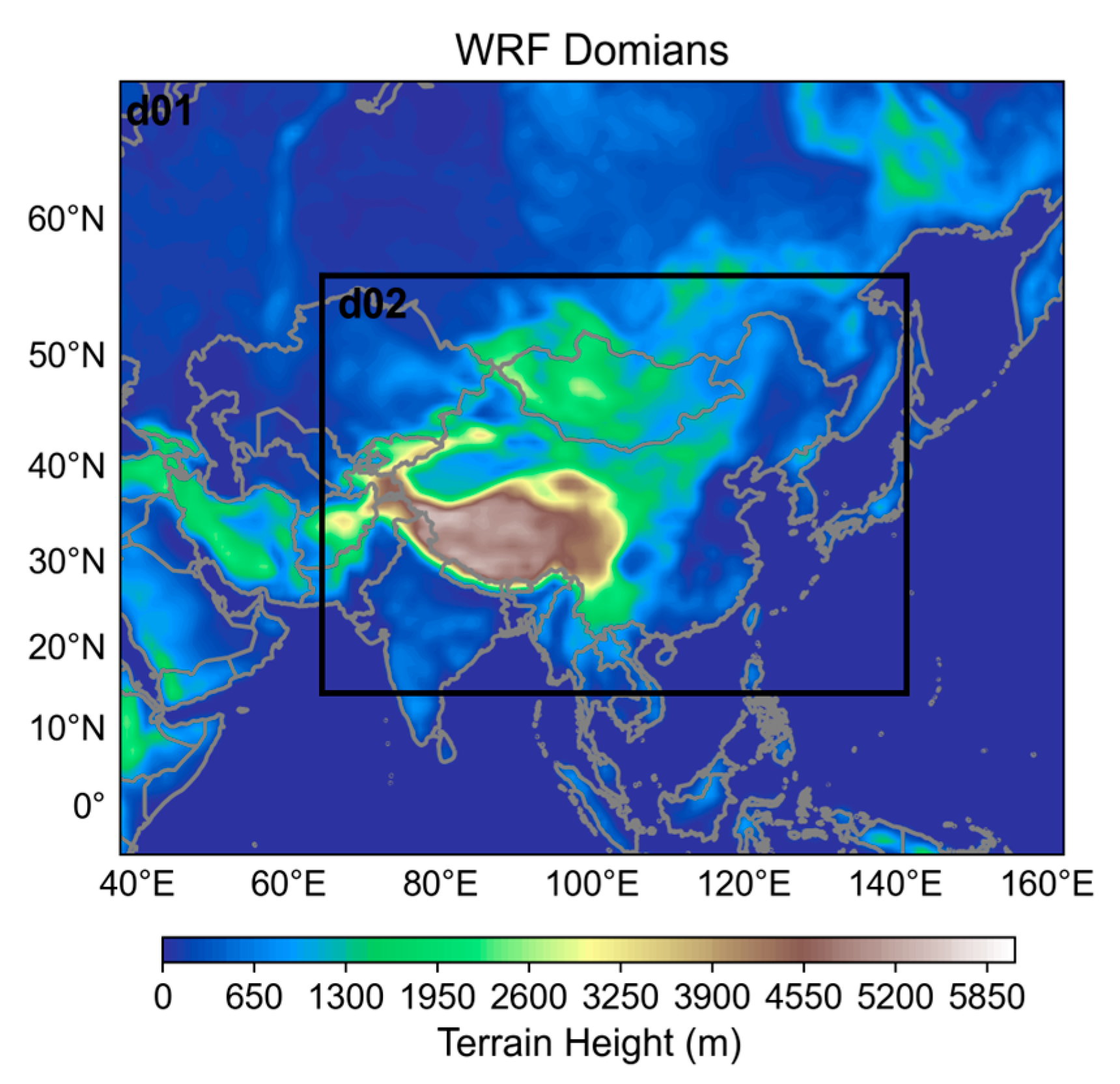
Figure 1. Configuration of the WRF-Solar and WRF-Solar EPS domains.
Remotesensing 17 03970 g001
Figure 2. Distribution of annual average GHI from (a) WRF-Solar, (b) WRF-Solar EPS, (c) satellite retrievals from December 2019 to November 2020.
Remotesensing 17 03970 g002
Figure 3. Intercomparison of the annual average (ac) bias, (df) RMSE, and (gi) MAE for the GHI from December 2019 to November 2020 derived from WRF-Solar and WRF-Solar EPS versus satellite retrievals. The column on the left shows the comparison results of WRF-Solar, the middle column shows the comparison results of WRF-Solar EPS, and the bar chart on the right shows the average values comparison of the corresponding statistical indicators in the regions of interest.
Remotesensing 17 03970 g003
Figure 4. Intercomparison of seasonal mean bias of GHI in the regions of SC (a,b), SCB (c,d), YZD (e,f), WC (g,h), and BTH (i,j) from December 2019 to November 2020. The left panels show the biases of WRF-Solar (blue bars) and WRF-Solar EPS (red bars) relative to satellite retrievals, while the right panels illustrate the bias differences between the two models (WRF-Solar EPS-WRF-Solar).
Remotesensing 17 03970 g004
Figure 5. Intercomparison of seasonal mean RMSE of GHI in the regions of SC (a,b), SCB (c,d), YZD (e,f), WC (g,h), and BTH (i,j) from December 2019 to November 2020. The left panels show the biases of WRF-Solar (dark blue bars) and WRF-Solar EPS (light blue bars) relative to satellite retrievals, while the right panels illustrate the bias differences between the two models (WRF-Solar EPS–WRF-Solar).
Remotesensing 17 03970 g005
Figure 6. Intercomparison of seasonal mean MAE of GHI in the regions of SC (a,b), SCB (c,d), YZD (e,f), WC (g,h), and BTH (i,j) from December 2019 to November 2020. The left panels show the biases of WRF-Solar (dark green bars) and WRF-Solar EPS (light green bars) relative to satellite retrievals, while the right panels illustrate the bias differences between the two models (WRF-Solar EPS–WRF-Solar).
Remotesensing 17 03970 g006
Figure 7. Intercomparison of monthly mean bias of GHI in the regions of SC (a,b), SCB (c,d), YZD (e,f), WC (g,h), and BTH (i,j) from December 2019 to November 2020. The left panels show the biases of WRF-Solar (dark blue bars) and WRF-Solar EPS (light blue bars) relative to satellite retrievals, while the right panels illustrate the bias differences between the two models (WRF-Solar EPS–WRF-Solar).
Remotesensing 17 03970 g007
Figure 8. Intercomparison of monthly mean RMSE of GHI in the regions of SC (a,b), SCB (c,d), YZD (e,f), WC (g,h), and BTH (i,j) from December 2019 to November 2020. The left panels show the biases of WRF-Solar (dark blue bars) and WRF-Solar EPS (light blue bars) relative to satellite retrievals, while the right panels illustrate the bias differences between the two models (WRF-Solar EPS–WRF-Solar).
Remotesensing 17 03970 g008
Figure 9. Intercomparison of monthly mean MAE of GHI in the regions of SC (a,b), SCB (c,d), YZD (e,f), WC (g,h), and BTH (i,j) from December 2019 to November 2020. The left panels show the biases of WRF-Solar (dark green bars) and WRF-Solar EPS (light green bars) relative to satellite retrievals, while the right panels illustrate the bias differences between the two models (WRF-Solar EPS–WRF-Solar).
Remotesensing 17 03970 g009
Figure 10. Distribution of annual average DIR from (a) WRF-Solar, (b) WRF-Solar EPS, and (c) satellite retrievals from December 2019 to November 2020.
Remotesensing 17 03970 g010
Figure 11. Intercomparison of the annual average (ac) bias, (df) RMSE, and (gi) MAE for the DIR from December 2019 to November 2020 derived from satellite retrievals versus WRF-Solar and WRF-Solar EPS models. The column on the left shows the comparison results of WRF-Solar, the middle column shows the comparison results of WRF-Solar EPS, and the bar chart on the right shows the average values comparison of the corresponding statistical indicators in the regions of interest.
Remotesensing 17 03970 g011
Figure 12. Intercomparison of seasonal mean bias of DIR in the regions of SC (a,b), SCB (c,d), YZD (e,f), WC (g,h), and BTH (i,j) from December 2019 to November 2020. The left panels show the biases of WRF-Solar (blue bars) and WRF-Solar EPS (red bars) relative to satellite retrievals, while the right panels illustrate the bias differences between the two models (WRF-Solar EPS–WRF-Solar).
Remotesensing 17 03970 g012
Figure 13. Intercomparison of seasonal mean RMSE of DIR in the regions of SC (a,b), SCB (c,d), YZD (e,f), WC (g,h), and BTH (i,j) from December 2019 to November 2020. The left panels show the biases of WRF-Solar (dark blue bars) and WRF-Solar EPS (light blue bars) relative to satellite retrievals, while the right panels illustrate the bias differences between the two models (WRF-Solar EPS–WRF-Solar).
Remotesensing 17 03970 g013
Figure 14. Intercomparison of seasonal mean MAE of DIR in the regions of SC (a,b), SCB (c,d), YZD (e,f), WC (g,h), and BTH (i,j) from December 2019 to November 2020. The left panels show the biases of WRF-Solar (dark green bars) and WRF-Solar EPS (light green bars) relative to satellite retrievals, while the right panels illustrate the bias differences between the two models (WRF-Solar EPS–WRF-Solar).
Remotesensing 17 03970 g014
Figure 15. Intercomparison of monthly mean bias of DIR in the regions of SC (a,b), SCB (c,d), YZD (e,f), WC (g,h), and BTH (i,j) from December 2019 to November 2020. The left panels show the biases of WRF-Solar (blue bars) and WRF-Solar EPS (red bars) relative to satellite retrievals, while the right panels illustrate the bias differences between the two models (WRF-Solar EPS–WRF-Solar).
Remotesensing 17 03970 g015
Figure 16. Intercomparison of monthly mean RMSE of DIR in the regions of SC (a,b), SCB (c,d), YZD (e,f), WC (g,h), and BTH (i,j) from December 2019 to November 2020. The left panels show the biases of WRF-Solar (dark blue bars) and WRF-Solar EPS (light blue bars) relative to satellite retrievals, while the right panels illustrate the bias differences between the two models (WRF-Solar EPS–WRF-Solar).
Remotesensing 17 03970 g016
Figure 17. Intercomparison of monthly mean MAE of DIR in the regions of SC (a,b), SCB (c,d), YZD (e,f), WC (g,h), and BTH (i,j) from December 2019 to November 2020. The left panels show the biases of WRF-Solar (dark green bars) and WRF-Solar EPS (light green bars) relative to satellite retrievals, while the right panels illustrate the bias differences between the two models (WRF-Solar EPS–WRF-Solar).
Remotesensing 17 03970 g017
Table 1. The parameterization schemes and experimental configurations used in this study for WRF-Solar and WRF-Solar EPS.
SettingWRF-SolarWRF-Solar EPS
microphysical schemeThompsonThompson
longwave and shortwaveradiation schemeRRTMGRRTMG
planetary boundary layer schemeMYNNMYNN
land surface schemeNoahNoah
cumulus cloud schemeGrell-3DGrell-3D
sub-grid-scale cloud schemeCLD3CLD3
AOD datamonthly climatologymonthly climatology
stochastic perturbationsoffon
Table 2. Abbreviations for selected areas and their latitude and longitude ranges.
Regions of InterestAbbreviationLatitudeLongitude
South ChinaSC17.5°N–26°N108°E–118°E
Sichuan BasinSCB27°S–34°N102°E–109°E
Yangtze River DeltaYZD27°N–34°N116°E–123.5°E
Western ChinaWC26°N–40°N82°E–98°E
Beijing-Tianjin-HebeiBTH35.5°N–43°N113°E–120°E
Disclaimer/Publisher’s Note: The statements, opinions and data contained in all publications are solely those of the individual author(s) and contributor(s) and not of MDPI and/or the editor(s). MDPI and/or the editor(s) disclaim responsibility for any injury to people or property resulting from any ideas, methods, instructions or products referred to in the content.