Article

Response of Vegetation to Extreme Climate in the Yellow River Basin: Spatiotemporal Patterns, Lag Effects, and Scenario Differences

1
College of Atmospheric Sciences, Lanzhou University, Lanzhou 730000, China
2
College of Oceanography and Space Informatics, China University of Petroleum (East China), Qingdao 266580, China
*
Author to whom correspondence should be addressed.
Remote Sens. 2025, 17(24), 3967; https://doi.org/10.3390/rs17243967
Submission received: 14 October 2025 / Revised: 25 November 2025 / Accepted: 2 December 2025 / Published: 8 December 2025
(This article belongs to the Section Ecological Remote Sensing)

Highlights

What are the main findings?
  • Under three CMIP6 SSP scenarios, the leaf area index (LAI) shows an increasing trend across the Yellow River Basin, with significant scenario-dependent spatial variations in both distribution patterns and responses to extreme climate indices.
  • Annual total wet-day precipitation, frost days, growing season length, summer days, and ice days are identified as key extreme climate indices driving LAI variability.
What are the implications of the main findings??
  • The relatively long time-lag and cumulative effects of climate extremes in arid/semiarid regions highlight vegetation vulnerability to prolonged climatic stress.
  • These findings provide a scientific basis for formulating region-specific ecological conservation and climate adaptation strategies in ecologically vulnerable watersheds.

Abstract

Extreme climates pose increasing threats to ecosystems, particularly in ecologically fragile regions such as the Yellow River Basin (YRB). Leaf area index (LAI) reflects vegetation response to climatic stressors, yet spatiotemporal dynamics of such responses under future climate scenarios remain poorly understood. This study examined LAI responses to extreme climatic factors across the YRB from 2025 to 2065, utilizing Coupled Model Intercomparison Project Phase 6 (CMIP6) outputs under three Shared Socioeconomic Pathways (SSP) scenarios. Partial least squares regression was performed using historical consistency-validated and future scenario LAI data alongside 26 extreme climate indices to identify extreme climate impacts on vegetation dynamics. Time-lag and cumulative effect analyses using Pearson correlation further quantified the potential impacts of extreme climate on future vegetation dynamics. Results indicate that the regionally averaged LAI in the YRB exhibits a consistent increasing trend under all three SSP scenarios, with linear rates of 0.0016–0.0020 yr−1 and the highest values under SSP5-8.5, accompanied by clear scenario-dependent spatial differences in LAI distribution and vegetation response to extreme climates, particularly in the lag and cumulative effects that depend on local hydro-climatic conditions. Partial least squares regression results identified annual total wet-day precipitation, frost days, growing season length, summer days, and ice days as the dominant extreme climate indices regulating LAI variability. In the arid and semiarid Loess Plateau regions, relatively long lag and cumulative effects imply vegetation vulnerability to delayed or prolonged climatic stress, necessitating enhanced soil and water conservation practices. These findings support region-specific ecological conservation and climate mitigation strategies for the YRB and other ecologically vulnerable watersheds.

1. Introduction

Under intensifying global climate change, climate disasters pose a serious threat to ecosystems. According to the World Meteorological Organization (WMO), the global mean temperature in 2024 was 1.55 °C above the preindustrial (1850–1900) average, with an uncertainty of ±0.13 °C based on six international datasets [1]. In the context of global warming, extreme climate events such as tropical cyclones, floods, and droughts are intensifying global ecological impacts [2,3].
Vegetation, a core ecosystem component, plays a critical role in shaping global carbon, water and energy cycles [4]. Extreme high temperatures can induce stomatal closure, reducing photosynthetic efficiency [5,6]. Cold waves and frost can directly kill newly emerging buds and leaves [7,8], and intense rainfall events can lead to root oxygen deficiency [9,10]. Long-term drought can significantly reduce plant water uptake capacity [11,12,13]. Extreme climate conditions disrupt the key physiological balance between photosynthesis and respiration, altering phenological traits, reshaping interspecific competition, and ultimately changing vegetation growth [14,15]. In recent decades, although some regions have shown sustained greening under broader climate and ecological restoration trends [16], climate extremes continue to exert substantial influence on the interannual variability and spatial heterogeneity of vegetation, as exemplified by the Yellow River Basin [17]. Among the various vegetation indices, the leaf area index (LAI) is a key biophysical parameter reflecting vegetation responses to climate change [18,19,20]. Thus, studying the effects of extreme climate on the LAI is crucial for predicting future ecosystem resilience and addressing the cascading effects of intensifying extreme climate change [21].
The Yellow River Basin (YRB), characterized by ecological fragility and high dependence on natural resources, exhibits complex vegetation dynamics shaped by both climate variability and anthropogenic activities [22,23,24,25]. The vegetation in the YRB is highly sensitive to extreme climates, affecting water resources, the carbon cycle, and biodiversity [26]. Previous studies have analyzed primarily historical trends, including LAI responses to past climate change [27] and the influence of individual extreme events on vegetation [17,28]. However, critical knowledge gaps remain regarding future vegetation dynamics in the YRB. Although research has examined vegetation responses to historical extreme events in the YRB [29,30], some limitations persist: (1) the spatiotemporal mechanisms by which specific extreme climate indices exert cumulative and lag effects on LAI remain poorly quantified, despite growing recognition of such temporal response processes [31,32]; and (2) systematic projections of LAI sensitivity to extreme climate indices under different Shared Socioeconomic Pathway (SSP) scenarios remain limited. Assessing future extreme climate impacts on the LAI in the YRB is critical for understanding vegetation dynamics and informing climate adaptation [33]. To address these gaps, this study adopts an integrated framework by analyzing spatiotemporal patterns to capture regional heterogeneity, quantifying lag and cumulative effects to reveal delayed ecological responses, and comparing three SSP scenarios to assess vegetation sensitivity under different emission pathways.
The Coupled Model Intercomparison Project Phase 6 (CMIP6) represents the latest generation of climate model intercomparison projects, offering substantial improvements over CMIP5. CMIP6 adopts a more federated organizational structure that addresses the increasingly broad scientific needs of the climate science community. Climate models are constantly being updated, as different modeling groups around the world incorporate higher spatial resolution, new physical processes and biogeochemical cycles. Additionally, CMIP6 employs the SSP framework to explore diverse future emission scenarios and socioeconomic development trajectories [34]. In this study, three representative SSP scenarios was selected to span a wide range of plausible futures: SSP2-4.5 represents a middle-of-the-road pathway with moderate mitigation efforts, SSP3-7.0 depicts a regional rivalry scenario with continued fossil fuel reliance, and SSP5-8.5 represents fossil-fueled development with intensive resource exploitation [35]. These scenarios were chosen to encompass different emission pathways and enable assessment of vegetation sensitivity across contrasting climate futures.
This study aims to clarify how vegetation in the YRB has responded and will respond to increasingly severe extreme climate by comparing historical and future LAI trends and their sensitivity to extreme climate indices under different scenarios. To achieve this, this study examines how future extreme climate indices affect LAI in the YRB, using projections from three CMIP6 SSP (SSP2-4.5, SSP3-7.0 and SSP5-8.5) [36]. LAI trends for 1982–2022 and 2025–2065 were quantified using the Mann–Kendall test with Sen’s slope estimator. On the basis of historical observational data and future scenario data, five key extreme climate indices significantly influencing LAI were identified through Partial Least Squares Regression (PLSR). Pearson’s correlation analysis was then performed on the future scenario datasets to examine the spatiotemporal responses of the LAI to the five identified extreme climate indices for 2025–2065. This framework highlights the study’s primary objective of linking key extreme climate indices with their cumulative and lag effects on vegetation, thereby providing robust theoretical support for regional ecosystem management and the formulation of climate adaptation strategies.

2. Materials and Methods

2.1. Study Area

As China’s second-longest river, the Yellow River drains approximately 794,600 km2 and spans nine provinces across eastern and western China [37] (Figure 1). The basin’s pronounced heterogeneity in climatic conditions and ecological environments arises from the diverse climatic zones and geomorphological features across its upper, middle, and lower reaches [38]. In recent years, the frequency of extreme climatic events in the YRB has markedly increased, with their spatial impacts progressively expanding [39,40], causing significant negative impacts on the basin’s ecosystems [28,30]. Under such circumstances, vegetation is essential for maintaining ecological balance, reducing climate stress, and supporting the resilience of ecosystem functions in the basin [41]. The ecological functions of vegetation include the regulation of evapotranspiration, reduction in soil erosion, enhancement of water and soil conservation, maintenance of the water–sediment balance of the YRB, and moderation of local temperature and humidity, and are critical to sustaining regional ecological integrity and supporting long-term sustainable development [42,43].

2.2. Methods

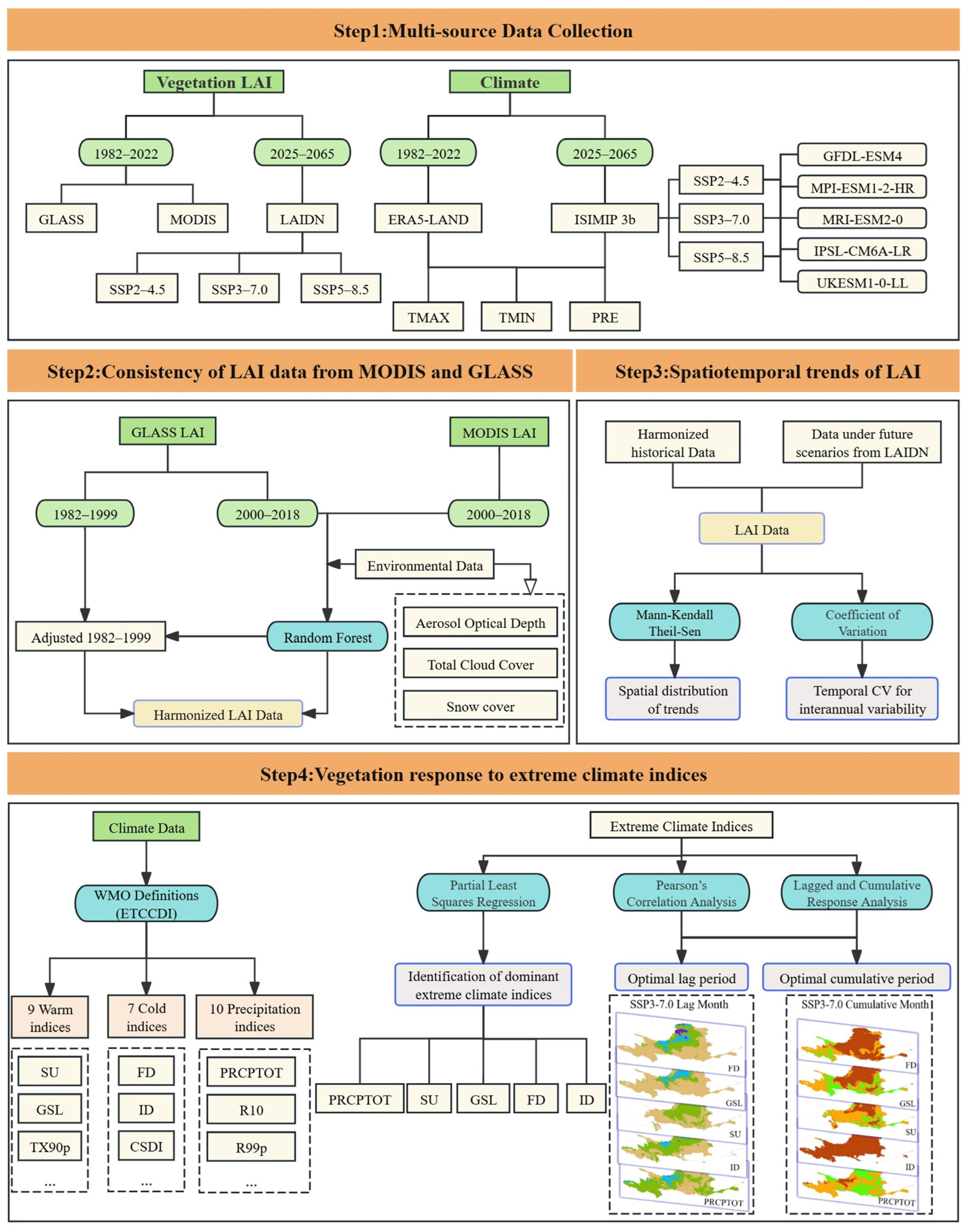
This study employed a systematic analytical framework to investigate vegetation responses to extreme climate in the YRB, as illustrated in Figure 2. The framework comprises four integrated components: (1) Multi-source Data collection: The acquisition and preprocessing of multisource data (Section 2.2.1); (2) Consistency of LAI data from MODIS and GLASS: MODIS and GLASS LAI datasets were harmonized through spatiotemporal consistency analysis (Section 2.2.2); (3) Spatiotemporal trends of LAI: Spatiotemporal patterns of LAI dynamics were quantified using Mann–Kendall tests and Sen’s slope estimators for both historical (1982–2022) and future (2025–2065) periods (Section 2.2.3); (4) Vegetation response to extreme climate indices: PLSR with variable importance in projection (VIP) scoring was applied to identify key extreme climate indices influencing LAI variability from 26 candidate indices (Section 2.2.4); Time-lag and cumulative effects of identified key drivers on vegetation dynamics were quantified through Pearson correlation analysis with temporal windows of 0–3 months (Section 2.2.5). This integrated approach enables comprehensive assessment of vegetation sensitivity to extreme climate under different scenarios, providing mechanistic insights into the temporal dynamics of ecosystem responses.

2.2.1. Multi-Source Data Collection

Multiple satellite-based LAI products have been developed using different retrieval approaches, including radiative transfer model inversion, vegetation index (VI)-based empirical algorithms, and machine learning methods. Common global LAI datasets—such as Moderate Resolution Imaging Spectroradiometer (MODIS) [44], Global Land Surface Satellite (GLASS) [45], and GEOV2 [46]—are generated using these techniques and provide long-term, spatially consistent observations widely used to assess vegetation responses to extreme climatic events. The historical vegetation LAI dataset used in this study was constructed through a spatiotemporal consistency analysis integrating the GLASS LAI product (1982–2018) and the MODIS MOD15A2H product (2000–2022) via a random forest (RF)-based approach. MODIS was used as the reference for consistency analysis owing to its well-validated retrieval algorithm and consistent multi-decadal temporal coverage, which together support robust cross-sensor calibration for vegetation–climate studies [47]. To ensure spatial comparability, both datasets were resampled to a uniform resolution of 0.05°. The aerosol optical depth (AOD) [48], snow depth estimate (SDE) [49], and total cloud cover (TCC) [50] were incorporated as auxiliary variables in the RF-based correction.
The future LAI dataset was derived from the LAIDN model developed by Li et al. [51], with a spatial resolution of 0.05°, monthly time steps, and a coverage period of 2025–2065, corresponding to a future period of equal duration to the historical record. This consistent temporal length enables a direct comparison of interannual LAI variability and ensures that the importance indices obtained from PLSR and correlation analyses remain representative across both historical and future periods, rather than being biased toward long-term projections.
Historical climate data, including daily maximum temperature, daily minimum temperature, and daily precipitation, were derived from the ERA5-Land high-resolution climate reanalysis dataset produced by the European Centre for Medium-Range Weather Forecasts (ECMWF) [52]. Future climate data were obtained from the Inter-Sectoral Impact Model Intercomparison Project phase 3b (ISIMIP 3b) bias-corrected CMIP6 dataset [53], covering three SSPs (SSP 2-4.5, SSP 3-7.0 and SSP5-8.5) and five models (GFDL-ESM4, IPSL-CM6A-LR, MPI-ESM1-2-HR, MRI-ESM2-0, and UKESM1-0-LL) with a daily temporal resolution. WFDE5 data over land merged with ERA5 data over the ocean were used as observational references for bias adjustment and statistical downscaling of the ISIMIP data, with the results subsequently validated [54]. On this basis, the dataset has been interpolated to 0.05° using bilinear interpolation to ensure consistency in spatial resolution with other datasets. The multimodel mean was then computed to reduce individual model bias and internal variability, and used to derive future extreme climate indices following the methodology of the Expert Team on Climate Change Detection and Indices (ETCCDI) under the WMO.

2.2.2. Consistency of LAI Data from MODIS and GLASS

In this study, MODIS LAI data for 2000–2022 were integrated with GLASS LAI data for 1982–2018. A spatiotemporal consistency analysis based on the RF algorithm and incorporating AOD, SDE, and TCC as auxiliary variables, was conducted to establish a MODIS–GLASS relationship model for the overlapping period of 2000–2018. This model was then applied to calibrate the GLASS data for the period of 1982–1999, resulting in a calibrated GLASS dataset at 0.05° spatial resolution. The performance of the harmonization was evaluated using the coefficient of determination (R2), producing a harmonized LAI dataset spanning 1982–2022.

2.2.3. Spatiotemporal Trends of LAI

The Mann–Kendall (MK) test [55,56] and Sen’s slope estimator [57] were employed to analyze spatiotemporal variations in the LAI under historical and future climate scenarios. The MK test is a non-parametric trend analysis method that is robust to non-normal distributions and widely used for long-term trend detection in environmental remote sensing data such as LAI [58,59]. In this study, it was applied to assess the statistical significance of trends. Trend magnitude was quantified using the Sen’s slope estimator, a non-parametric method robust to outliers [60,61]. This estimator is commonly paired with the MK test and provides reliable estimates for LAI datasets characterized by spatial heterogeneity and temporal variability. In addition, the coefficient of variation (CV) [62] was employed to assess the interannual variability of LAI, reflecting the stability and consistency of vegetation dynamics in response to extreme climate. Higher CV values indicate stronger interannual fluctuations in vegetation, whereas lower values reflect greater stability [63].

2.2.4. PLSR

The 26 extreme climate indices used in this study follow the standardized definitions established by the WMO ETCCDI. Due to the large number of indices, their complete definitions are provided in Supplementary Materials Table S1. The five key indices used in this study are: PRCPTOT (annual total wet-day precipitation), FD (frost days), GSL (growing season length), SU (summer days), and ID (ice days). This study applied the PLSR algorithm [64,65] to quantify the variable importance in projection (VIP) of each index across different scenarios. PLSR was selected for its ability to effectively handle multicollinearity among the 26 climate indices through orthogonal latent variables while providing VIP metrics to objectively identify key drivers [66,67]. For 1982–2022, the analysis was based on spatiotemporally harmonized LAI derived from historical satellite observations, and extreme climate indices calculated from the ERA5-Land high-resolution climate reanalysis dataset. For the period 2023–2065, the LAI was simulated using the LAIDN model [51], and the extreme climate indices were calculated based on bias-corrected multimodel ensemble climate projections from ISIMIP3b, spatially resampled to a unified resolution under three SSP scenarios. The performance of the PLSR models was evaluated primarily based on the coefficient of determination (R2) for the response variable LAI [68]. By applying a VIP threshold, key extreme climate factors with an explanatory effect on the variability in the vegetation LAI (VIP > 1) were selected, thereby avoiding the interference of multicollinearity and establishing a quantitative response relationship between extreme climate and vegetation dynamics.
V I P j = p h = 1 m R 2 ( y , t h ) w j h 2 / h = 1 m R 2 ( y , t h ) 1 / 2
where p denotes the total number of independent variables; m denotes the number of latent variable components; th denotes the h-th latent variable; R2 (y, th) denotes the coefficient of determination between y and th; and wih denotes the weighting coefficient of the j-th independent variable in constructing the h-th component. Notably, the higher the VIP value is, the more significant the explanatory effect is. When the VIP value exceeds 1, the corresponding factor is considered to have a significant explanatory effect, contributing to improved model robustness and predictive accuracy.

2.2.5. Time Lag Effect and Cumulative Effect on the Future Vegetation LAI

On the basis of the screening criteria established in Section 2.2.4, extreme climate indices that were significantly correlated with the LAI and could be computed on a monthly basis were selected. Pearson’s correlation analysis [69] was conducted with an analysis window set from 0 to 3 months [70], to examine the absolute value of the correlation coefficient (|r|) between the LAI in the current month and the climate indices in the analysis window at the 0.05 significance level. In regions where climate indices remained persistently at zero, correlation with the LAI could not be computed. This method quantifies the lagged and cumulative responses of the LAI to extreme climate indices, identifying optimal lag and cumulative periods [71,72], thus enabling a comprehensive analysis of vegetation response timing and magnitude to extreme climate conditions [73,74]. All data processing and visualization were performed using Python 3.9 (open-source), R 4.2.2 (open-source), and ArcGIS 10.8 (licensed academic software).

3. Results

3.1. Consistency of the LAI Data from MODIS and GLASS

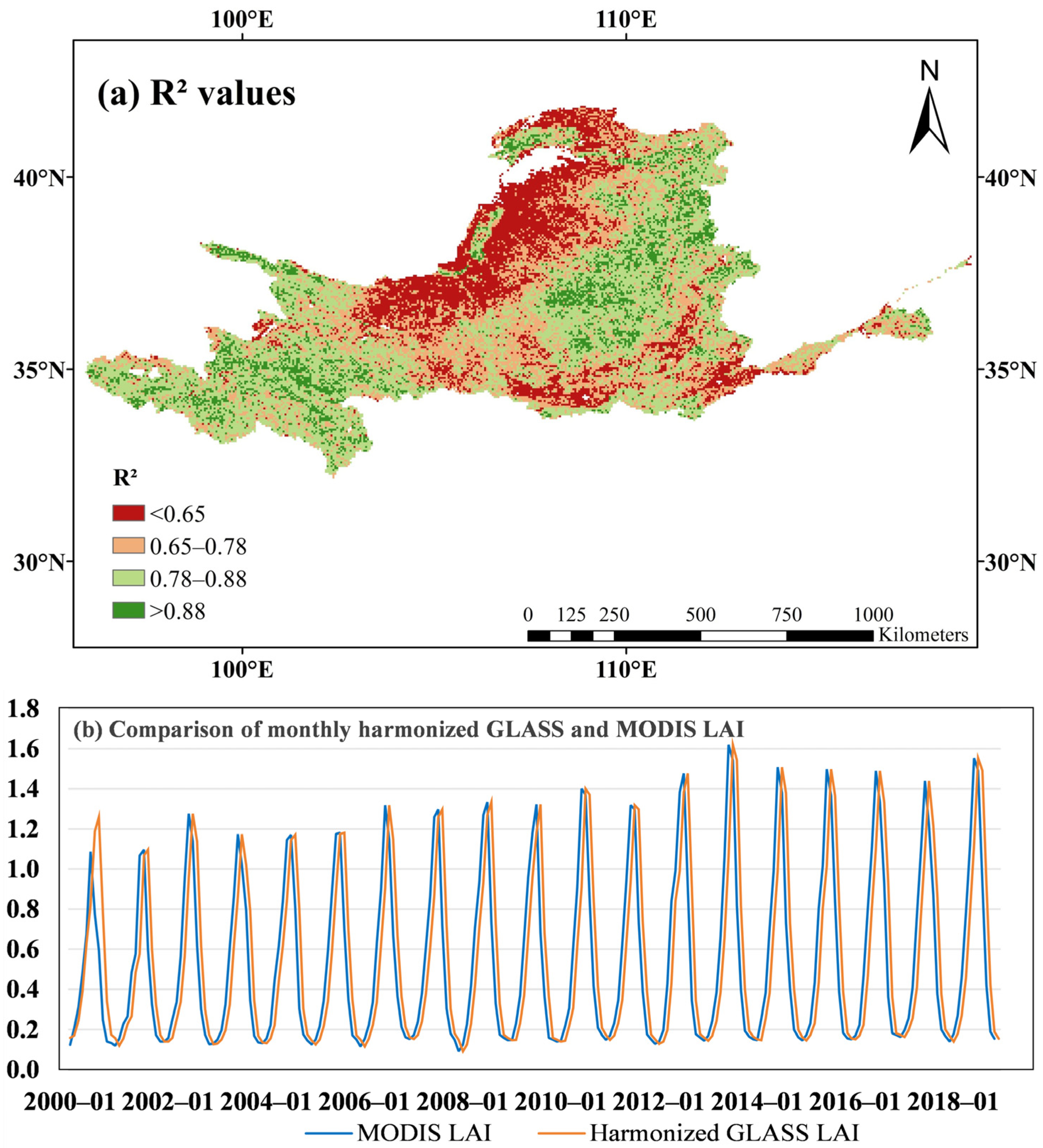
The RF algorithm was applied to correct and assess the spatiotemporal consistency between the MODIS and GLASS LAI datasets, with the model performance evaluated using R2. Pixels with R2 values less than 0.65 were excluded from correction, and the original GLASS LAI values were retained in these areas. A total of 6294 pixels (approximately 155,724.83 km2) were excluded, accounting for 20.03% of the YRB area. The model achieved an average R2 of 0.747, reflecting strong explanatory capacity overall. As shown in Figure 3, most corrected pixels exhibited R2 values between 0.65 and 0.89, indicating a generally high model fit, and the regional average monthly values also exhibited strong consistency. Spatially, relatively lower R2 values were concentrated in the northwestern Loess Plateau, indicating weaker performance in that region. Further examination using high-resolution remote sensing imagery and land-use datasets showed that these low-accuracy pixels are primarily associated with surface types characterized by very sparse or absent vegetation—such as bare soil, mining zones, and construction land—where LAI retrieval is inherently more uncertain, resulting in reduced consistency in correction.
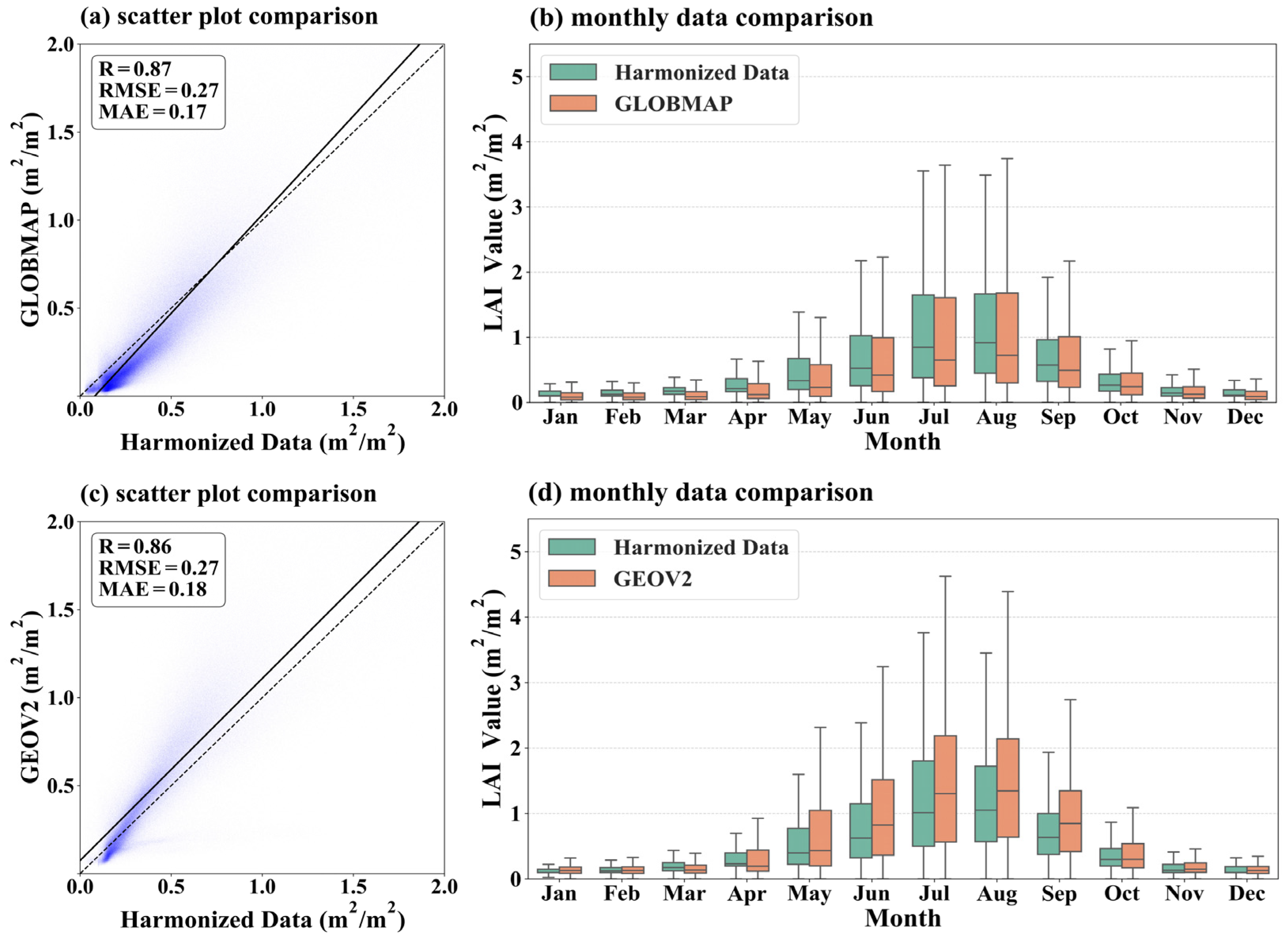
To evaluate the accuracy and reliability of the harmonized LAI dataset developed in this study, a comparative validation was conducted using two widely recognized reference products: Long-term Global Mapping (GLOBMAP) LAI product [75] (1982–2020) and GEOV2 (1999–2020). Figure 4 presents the results of this assessment. At the pixel level, scatterplots with linear regression and 1:1 reference line were used to quantify consistency. In these plots, the blue color density indicates data concentration, while the solid and dash lines represent the linear regression fit and the 1:1 reference line, respectively. The harmonized LAI shows strong agreement with both GLOBMAP and GEOV2, yielding correlation coefficients of 0.87 and 0.86, respectively, with root mean square error (RMSE) values of 0.27 and mean absolute errors (MAE) below 0.18. In addition, monthly boxplots reveal highly consistent temporal distributions and seasonal cycles across datasets, including the peak growth period from June to August. Overall, these results demonstrate that the harmonized long-term LAI series provides robust and credible estimates that align well with established benchmark products.

3.2. Spatiotemporal Patterns of LAI Trends Under Historical and Future Climate Scenarios

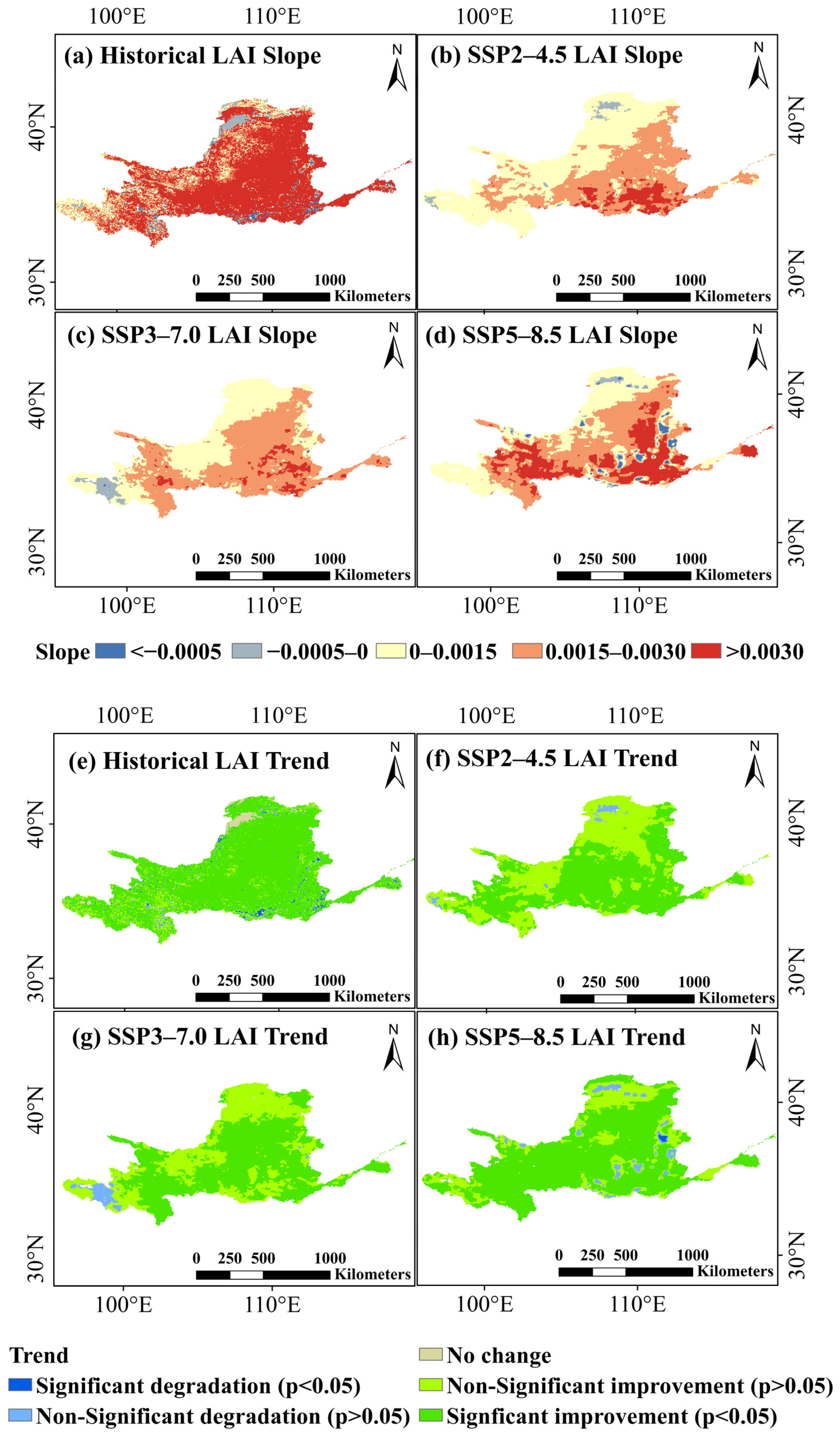
The MK test and Sen’s slope estimator were used to analyze the temporal change characteristics of the vegetation LAI during the historical period (1982–2022) and under three future SSP scenarios (2025–2065). The spatial distributions of the LAI trends are shown in Figure 5a–d. During the historical period, 83.43% of the YRB exhibited a significant increasing trend (p < 0.05). Under the future scenarios SSP2-4.5, SSP3-7.0, and SSP5-8.5, the percentages of the basin with a significant increase in LAI were 56.14%, 58.63%, and 74.90%, respectively, with particularly notable increases observed in the downstream regions. In contrast, under the SSP5-8.5 scenario, the LAI significantly decreased in parts of the southeastern midstream region. Sen’s slope analysis revealed that during the historical period, 96.12% of the basin exhibited vegetation improvement, as indicated by positive slope values (slope > 0). Moreover, under the three future emission scenarios, the proportions of improvement areas (slope > 0) are projected to be 98.55%, 97.24%, and 96.03%, respectively (Figure 5e–h). Overall, vegetation improvement is projected to persist under all the scenarios; however, under SSP5-8.5, the spatial extent of improvement slightly decreases. Compared with the historical period, the proportion of improvement areas increases under SSP2-4.5 and SSP3-7.0, but slightly declines under SSP5-8.5. Notably, in the southeastern midstream region, the area with a significant decrease in the LAI expands under SSP5-8.5, indicating a heightened risk of vegetation degradation.
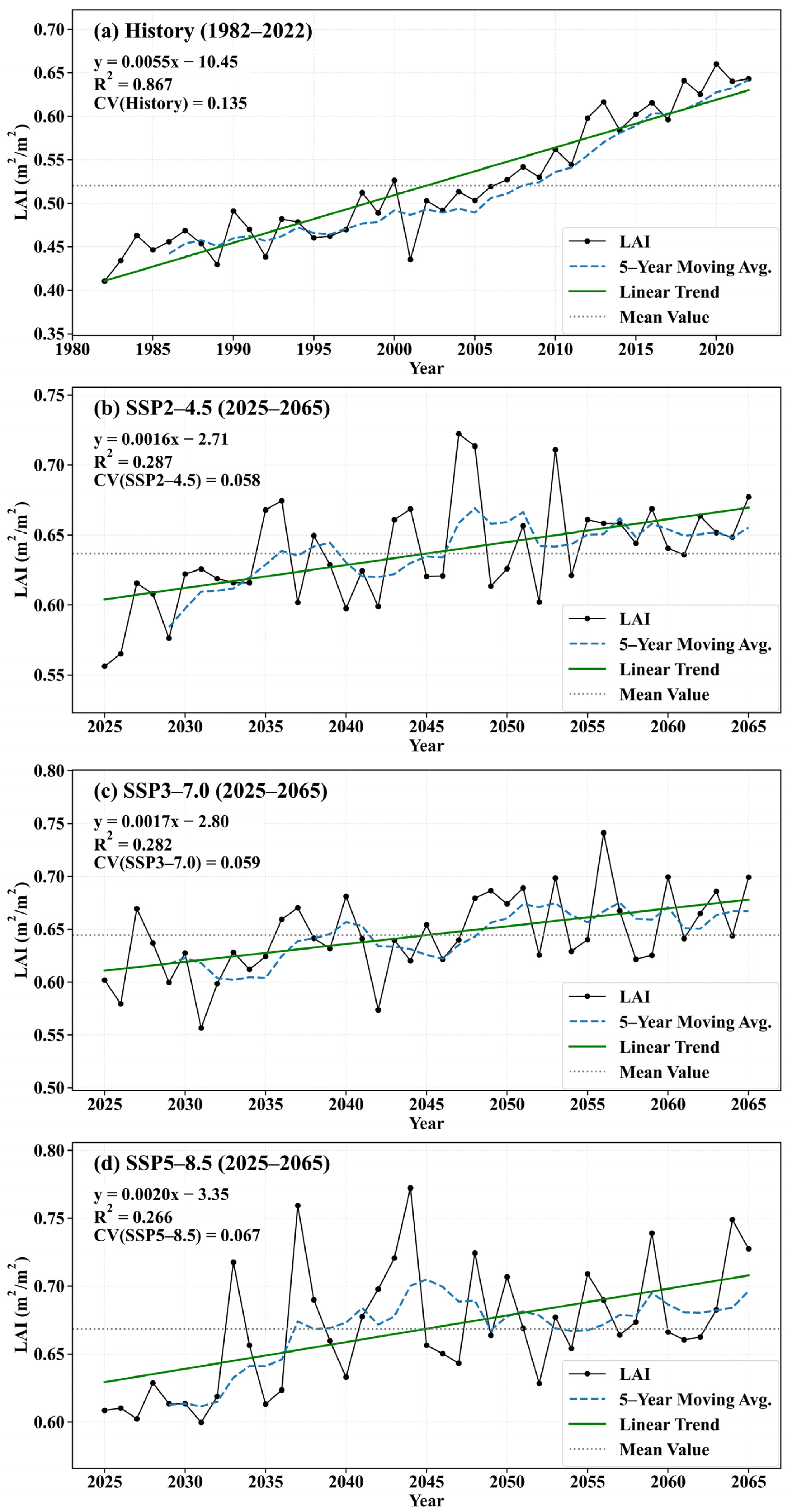
The analysis of the CV values derived from long-term LAI time series (Figure 6) showed that the CV value during the historical period was 0.135, whereas the CV values under the three future climate scenarios were 0.058, 0.059, and 0.067, respectively. Among future scenarios, SSP5-8.5 displayed the highest relative variability, though still lower than the historical period. The 5-year moving average effectively smooths short-term variability and reveals underlying long-term trajectories. During the historical period, the moving-average curve shows a steady upward trend, and similar long-term increases are observed across all future scenarios. Larger year-to-year fluctuations under higher-emission scenarios such as SSP3-7.0 and SSP5-8.5, and their moving-average curves display stronger rising tendencies, indicating that elevated climate forcing enhances both the magnitude of interannual fluctuations and the rate of long-term vegetation growth.

3.3. Key Extreme Climate Drivers of LAI Dynamics

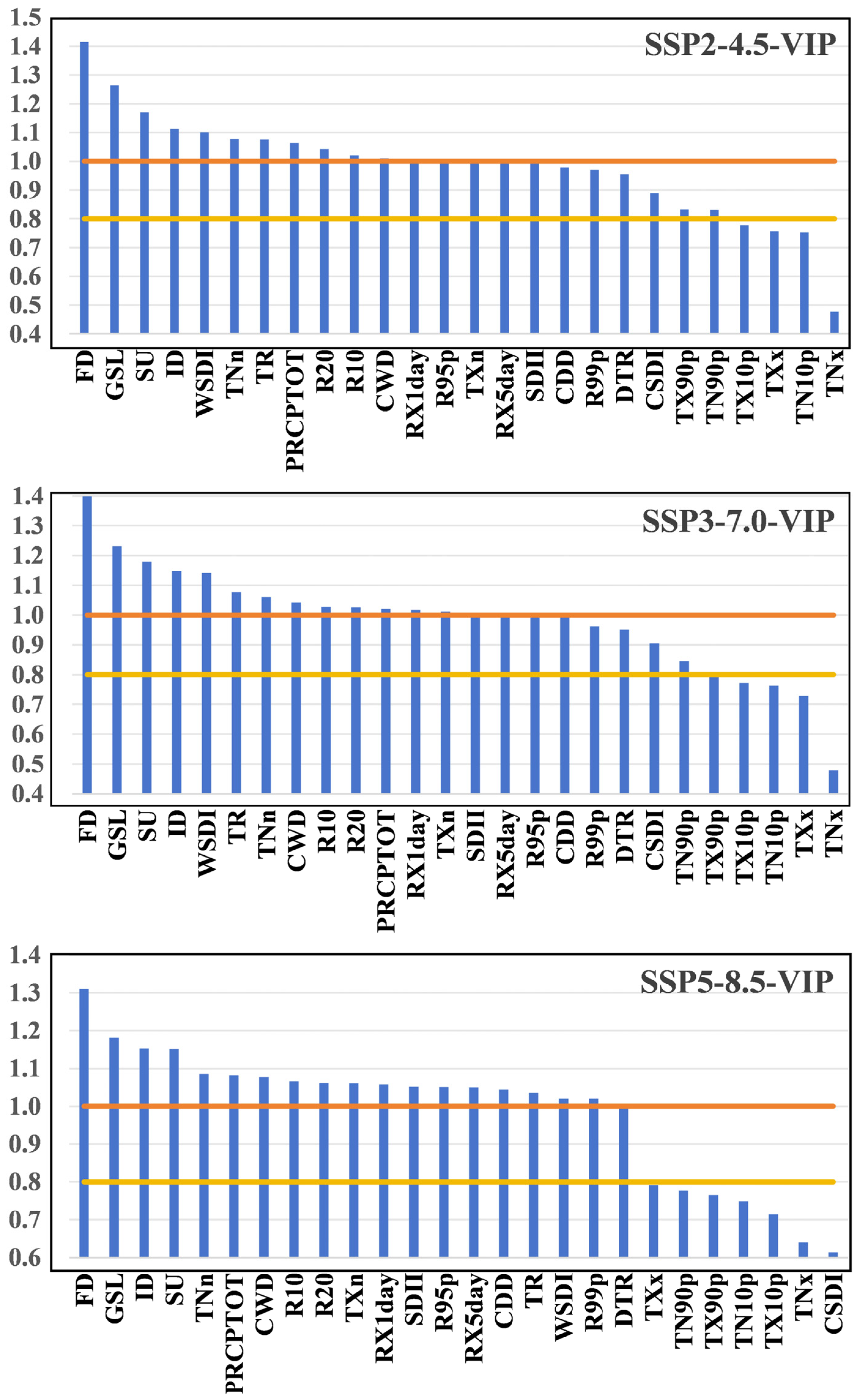
Using long-term time series data under three different scenarios—where this period corresponds to consistent historical observations—PLSR method and VIP scores were employed to quantify the driving effects of extreme climate indices on vegetation LAI. As shown in Table 1, PLSR models were constructed based on long-term time series data under the historical period and three SSP scenarios. Under the three scenarios, each model extracted six potential components, with model predictive capabilities (R2) of 0.805, 0.805, and 0.824, respectively, all exceeding 0.80, demonstrating satisfactory model performance. Table 1 presents the Beta coefficients (β) for the five indices based on their importance ranking. Positive beta coefficients indicate that an increase in the corresponding climate index is associated with enhanced vegetation growth and higher LAI values—for example, higher SU generally promotes photosynthetic activity and canopy development. In contrast, negative coefficients reflect indices that exert suppressing effects on vegetation, such as FD and ID, which can inhibit leaf formation, damage plant tissues, and reduce canopy cover.
The VIP scores of all the predictors are shown in Figure 7. Four temperature-related indices—FD, GSL, SU, and ID—consistently ranked among the top four across all three scenarios, with VIP scores greater than 1, indicating that these variables strongly and stably influence the vegetation LAI. Since vegetation growth is jointly regulated by temperature and precipitation, incorporating precipitation indices is also essential. Among all the precipitation-related indices, PRCPTOT ranked the highest when evaluated across all three scenarios, with VIP scores exceeding 1, demonstrating a strong explanatory power for LAI variations within each scenario. Taken together, and considering the compatibility of temporal resolution as well as the necessity of integrating both temperature and precipitation as key climatic drivers, five indices were ultimately selected for subsequent lagged cumulative analysis: one precipitation index (PRCPTOT) and four temperature-related indices (FD, GSL, SU, and ID). As shown in Table 1, the results revealed that across all scenarios, FD consistently exerted a strong negative impact on LAI, with this effect intensifying under higher emission scenarios (coefficients of −0.44, −0.60, and −0.67, respectively). In contrast, ID showed relatively weaker negative impacts. Under the SSP370 scenario, the index exhibited maximum (β = −0.25), compared with the other scenarios. SU was positively correlated with the LAI.

3.4. Time Lag Response of the LAI to the Extreme Indices

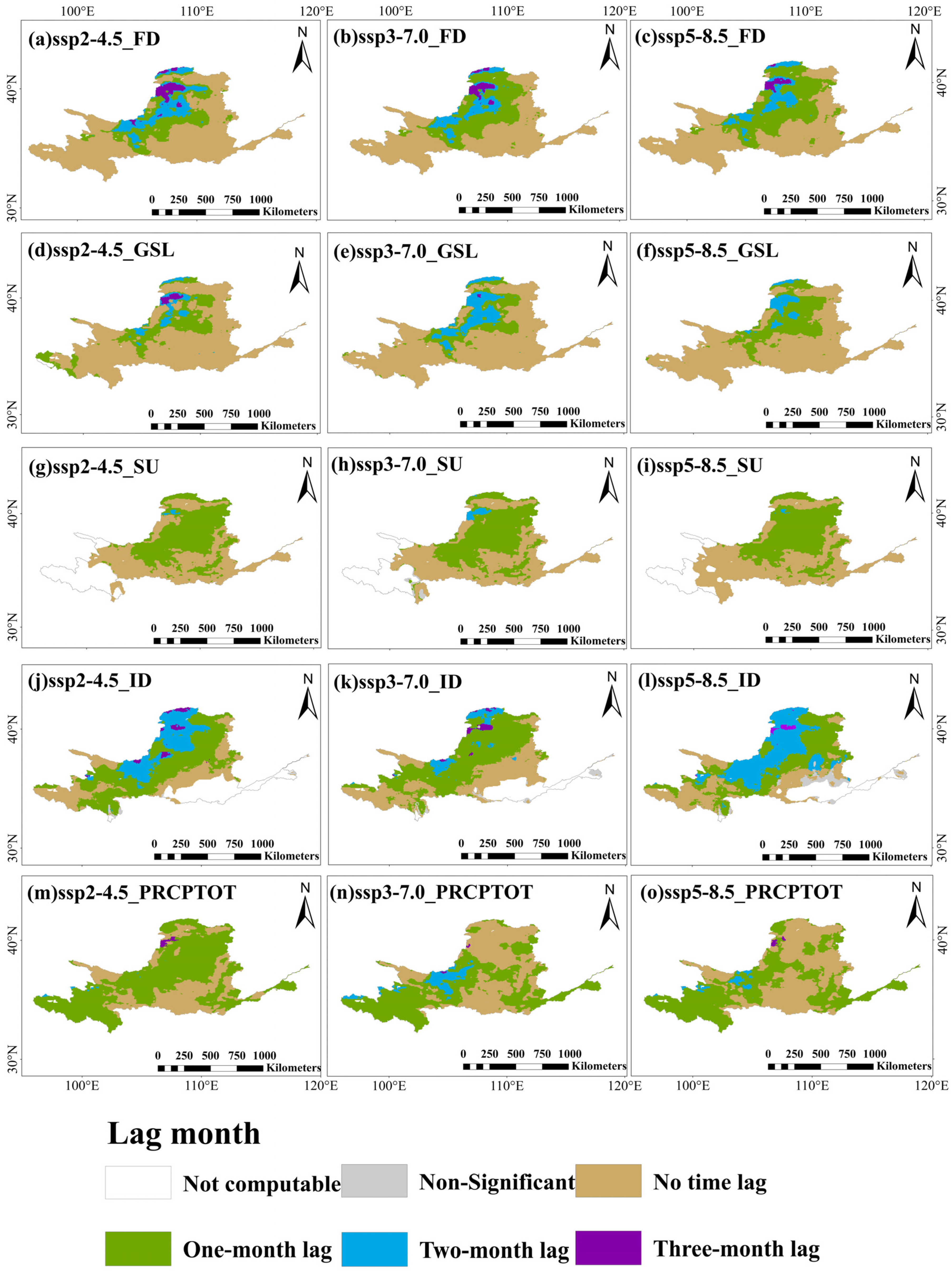
Figure 8 shows the spatial and temporal characteristics of lagged responses of vegetation LAI to extreme climate indices under three future scenarios in the YRB. Figure 8a–c show the lag effects of FD, (d)–(f) those of GSL, (g)–(i) those of SU, (j)–(l) those of ID, and (m)–(o) those of PRCPTOT. Different colors represent different lag-month responses, indicating how vegetation sensitivity varies with increasing temporal delays under each scenario. Among them, the first four indices are temperature-related, and the last index is related to precipitation. Among the temperature indices, two are warm indices (GSL and SU) and two are cold indices (FD and ID). Overall, from SSP2-4.5 to SSP5-8.5, the influences of the extreme climate indices on vegetation varied across the three scenarios.
The FD and GSL indices had significant impacts on more than 99% of the basin, with only a small portion of the upstream region showing no significant correlation. In terms of lag effects, both indices exhibited a 0-month lag in the upstream, eastern and southern middle reaches, at the northern bend (“Ji”-shaped bend) of the Yellow River, and in the downstream regions. However, in the Loess Plateau regions within the upper reaches and the southern Inner Mongolian Plateau, the lag time increased gradually from southeast to northwest. From the SSP2-4.5 scenario to the SSP5-8.5 scenario, the area experiencing a 3-month lag decreased.
In all three scenarios, certain upstream regions of the basin exhibited areas where the correlation for the SU index could not be calculated. This limitation arises because these regions, located on the Tibetan Plateau, have high elevations where the number of days with maximum temperatures above 25 °C remains zero, making the correlation between SU and LAI infeasible. No 3-month lag effects were detected in the basin. The largest area with a 2-month lag was observed under the SSP3-7.0 scenario. A 1-month lag was identified in the Loess Plateau regions within the upper reaches and in the southern Inner Mongolian Plateau, whereas all the other regions exhibited no lag.
Like the SU index, the ID index revealed regions where correlations could not be calculated, primarily in the southern middle reaches and downstream areas of the YRB. This is because these regions, which are located at lower latitudes and near the ocean, experience strong oceanic moderation, resulting in zero days with maximum temperatures below 0 °C and making the correlation between ID and LAI infeasible.
In the Yellow River source area, the lag for ID was predominantly 0 months. However, areas exhibiting a 2-month lag were primarily concentrated in the central Loess Plateau and southern Inner Mongolian Plateau regions. Furthermore, the lag effects of the precipitation index were pronounced across the entire basin, demonstrating greater spatial variation among scenarios compared to the temperature indices.
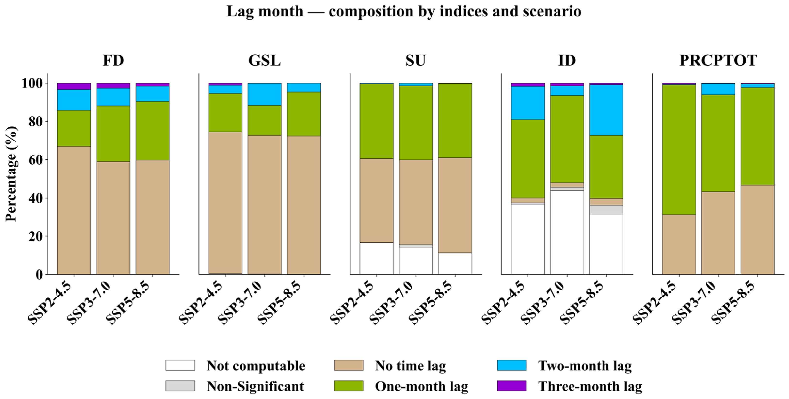
The proportion of pixels corresponding to the lag months for the five indices under the three scenarios in the YRB are shown in Figure 9. The bar chart comparison reveals distinct differences between lag and accumulation effects across indices and scenarios. The proportions of areas with a 3-month lag for FD were 3.33%, 2.66%, and 1.59% under the three scenarios, respectively. For GSL, the proportion of areas with a 3-month lag decreased across the three scenarios: 1.09%, 0.10%, and 0, with no areas showing a 3-month lag under the SSP5-8.5 scenario. The longest lag effect for SU was 2-month lag, which occurred in the northern basin, covering only small areas, with proportions of 0.40%, 1.37%, and 0.20% under the three scenarios, respectively. Under the three climate scenarios, for ID, areas with a 2-month lag accounted for 17.38%, 5.15%, and 26.47% of the basin, respectively. Regarding precipitation lag patterns, no-lag regions covered 31.23%, 43.23%, and 46.72%, respectively, while 1-month lag regions represented 67.83%, 50.63%, and 50.94% of the basin area, respectively. In the source area under SSP2-4.5, only 0.31% of the basin exhibited a 2-month lag, and notably, the 2-month lag area decreased from 5.96% under SSP3-7.0 to 1.96% under SSP5-8.5. The three-month lag areas were minimal across all scenarios, accounting for merely 0.59%, 0.18%, and 0.39%, respectively. Overall, GSL exhibits the shortest lag time, with the no time lag covering the largest area among all the indices. SU was the only index without a three-month lag, whereas the other four indices show the highest proportion of three-month lags under the SSP2-4.5 scenario.

3.5. Time Cumulative Response of the LAI to the Extreme Indices

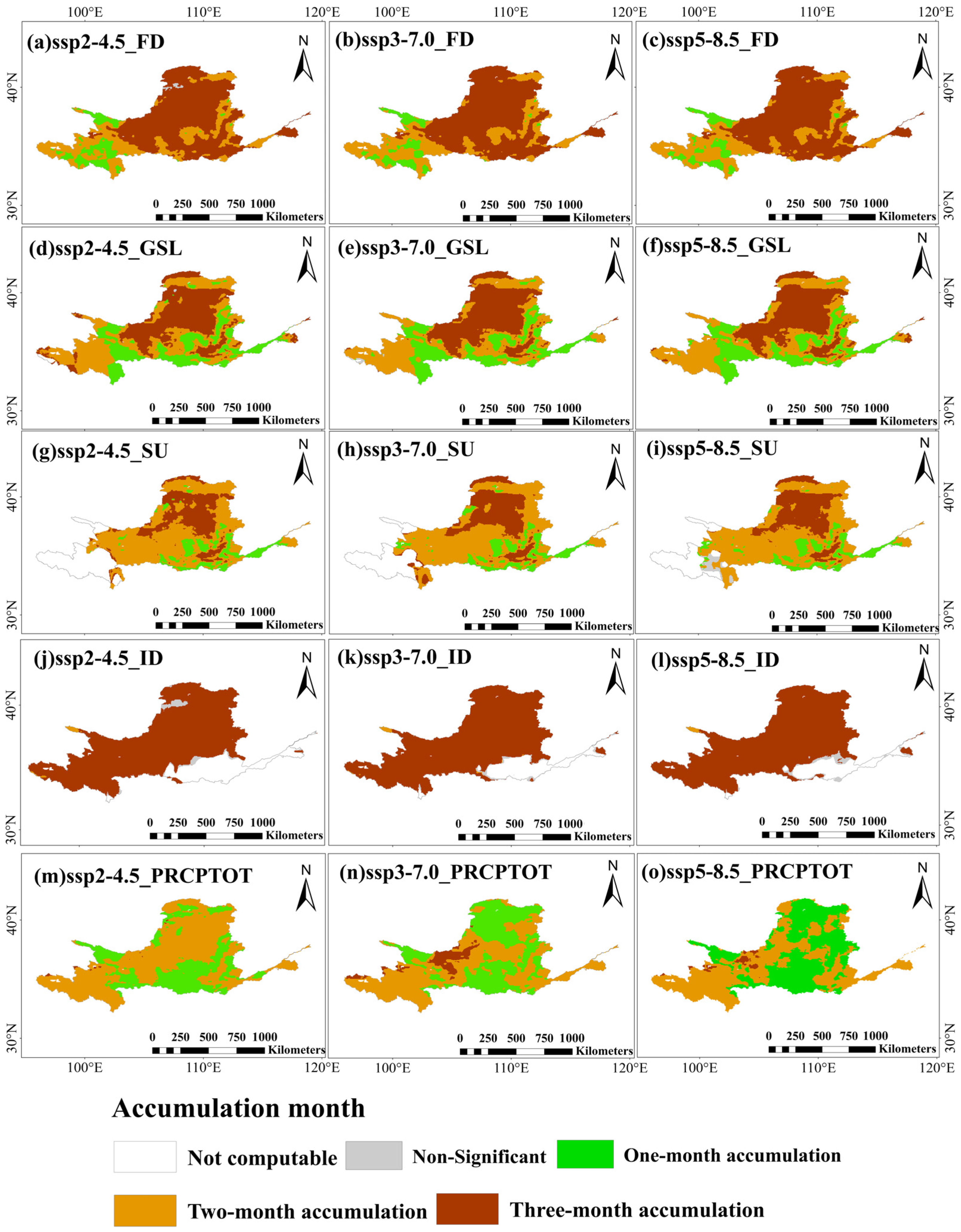
In terms of cumulative effects, as shown in Figure 10, the five indices exhibited distinct spatial patterns across different regions. For FD, a 1-month cumulative effect occurred in the river source area, while most of the Loess Plateau regions within the upper reaches and the southern Inner Mongolian Plateau displayed a 3-month cumulative effect. Meanwhile, the areas with a 2-month effect were fragmented and scattered across the basin. For GSL, the 2-month cumulative effect showed a relatively stable spatial distribution across the three SSP scenarios. The 3-month cumulative effect of SU was primarily concentrated in the Loess Plateau and the southern Inner Mongolian Plateau, with some distribution extending to the upstream and southern middle reaches. In contrast, the 2-month effect occurred mainly in other parts of the upper and middle reaches, whereas the 1-month effect was fragmented and concentrated in the southern middle reaches and downstream areas. For ID, the 2-month cumulative effect was observed mainly in Qinghai Province, while in most parts of the basin, the cumulative effect persisted for 3 months. Regarding PRCPTOT, cumulative effects also exhibited distinct spatial patterns and scenario-dependent characteristics. Under the SSP2-4.5 scenario, areas with 1-month cumulative effects showed similar distribution to areas with no time lag, and areas with 2-month cumulative effects resembled those with 1-month time lag. Under the SSP3-7.0 and SSP5-8.5 scenarios, however, the areas with 1-month cumulative effects were primarily distributed in northeastern Qinghai and the Loess Plateau, while areas with 2-month cumulative effects were mainly located in the river source area, downstream areas, scattered areas in the middle reaches, and southern Inner Mongolia Plateau.
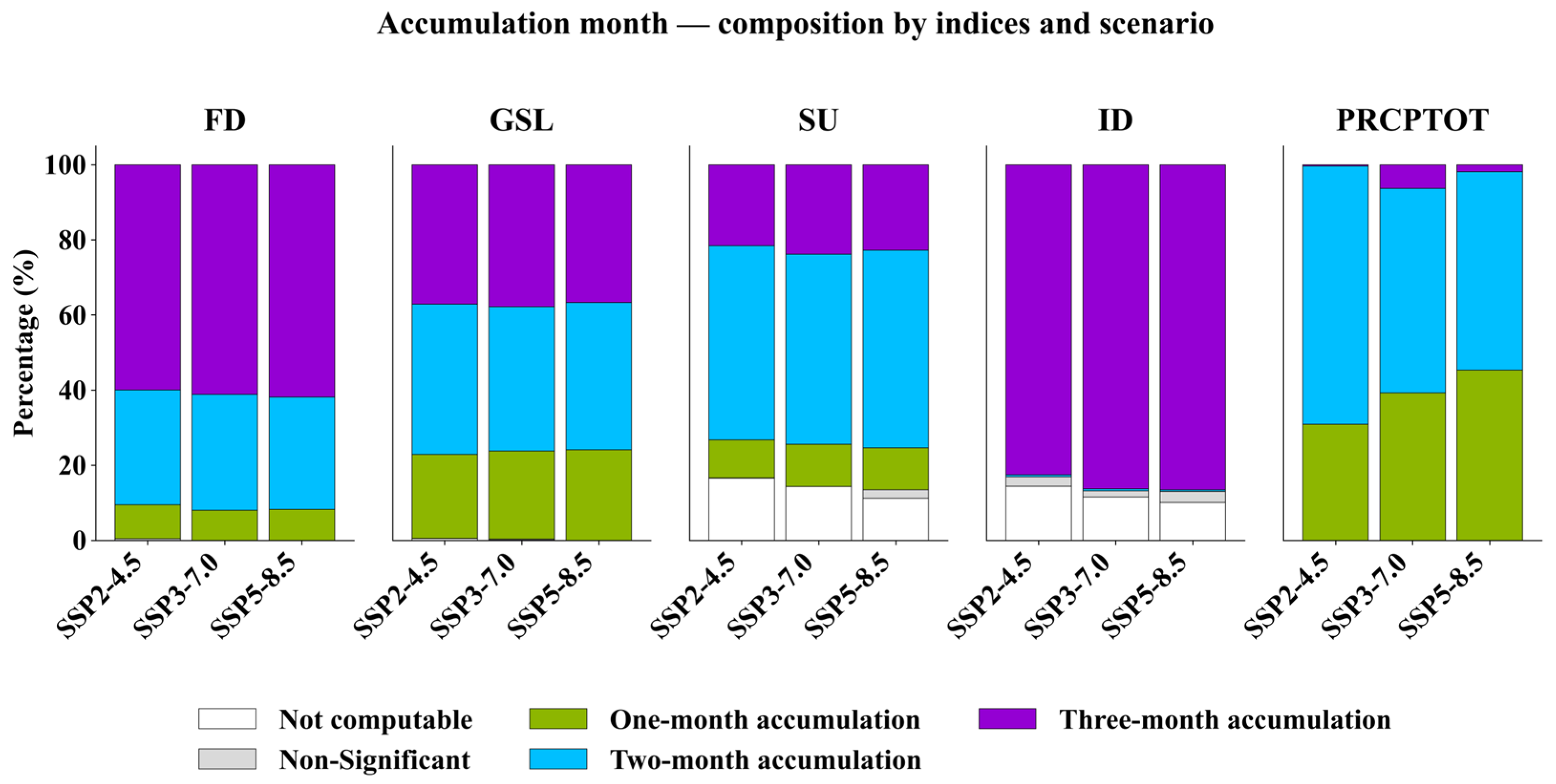
Figure 11 presents the proportion of pixels associated with different accumulation months for the five indices across the three scenarios in the YRB. Quantitatively, the GSL index results demonstrated that the 3-month effect areas exhibited minimal variation, accounting for 37.09%, 37.79%, and 36.68% of the basin under the three scenarios, respectively. Conversely, the extent of the 1-month effect increased progressively, covering 22.35%, 23.41%, and 24.13% of the basin under SSP2-4.5, SSP3-7.0, and SSP5-8.5, respectively. For ID, the 2-month cumulative effect showed a decreasing trend across the scenarios, accounting for 1.73%, 1.42%, and 0.81%, respectively. For PRCPTOT, under the SSP2-4.5 scenario, the areas with 3-month cumulative effects were limited, covering only 0.35% of the basin and mainly located in the source region. Furthermore, the spatial pattern of areas with 3-month cumulative effects resembled that of areas with 2-month time lag, reaching a maximum under the SSP3-7.0 scenario (6.32%) and subsequently declining to 1.90% under the SSP5-8.5 scenario. Overall, the cumulative effects varied less across the three scenarios, with ID exhibiting the longest accumulation duration. Except for SU and PRCPTOT, the accumulation duration of the remaining indices tends to increase. When the lag and accumulation effects for the same index were compared, FD shows similar proportions between the no-lag months and three-month accumulation months, while the precipitation-related indices displayed comparable patterns in terms of both the lag and accumulation effects.

4. Discussion

4.1. Long-Term LAI Trends

This study aims to clarify how vegetation in the YRB has responded and will respond to increasingly severe extreme climate by comparing historical and future LAI trends and their sensitivity to extreme climate indices under different scenarios. The spatiotemporal trend analysis shows that the annual average LAI across the YRB increased during the historical period (1982–2022) and under the three SSP scenarios (2025–2065), with interannual variability. The upward trend observed during the historical period (slope = 0.0055 yr−1) can be largely attributed to ecological restoration initiatives and adaptive vegetation recovery strategies implemented by the Chinese government [76]. Future spatial pattern analysis indicated that under scenarios with rising carbon emissions, the fertilization effect of elevated CO2 concentrations may increase vegetation growth [77], expanding areas with higher LAI values across much of the basin. However, with increasing scenario severity, small clusters of vegetation decline are projected to expand in the eastern and southern central reaches. This localized degradation may result from rising temperatures and intensified evaporation, which promote soil salinization and vegetation deterioration, thereby reducing LAI. Our findings of overall LAI increases are consistent with previous studies reporting widespread greening trends across the YRB [78,79]. The proportion of areas exhibiting significant LAI increases during the historical period in this study (83.43%) is higher than the 72.2% reported in [80]. This difference may result from variations in the study periods, as differences in temporal coverage can affect the estimated magnitude of long-term trends, even when the spatial patterns remain generally consistent.
During the historical period, the CV of the LAI across the entire basin was 0.135, indicating significant interannual variability in the YRB from 1982 to 2022. This variability may be closely related to the implementation of environmental protection and ecological restoration policies, such as the Grain for Green program, which have significantly improved the ecological environment of the basin. In the long term, under the three future scenarios, the CV of the LAI remained below 0.1, indicating relatively low interannual variability in the YRB. The lower CV values may reflect the proportionally smaller year-to-year deviations relative to the increasing mean LAI values, suggesting enhanced temporal stability of vegetation dynamics.

4.2. Vegetation Response to Extreme Climate Indices

The PLSR method was used to identify four temperature-related extreme climate indices and one precipitation-related index which, when synthesized across all three scenarios, had the most significant impacts on the vegetation LAI. The β coefficients of the PLSR model further support this conclusion: FD exerted the strongest and consistently negative influence, which intensified under higher-emission scenarios, underscoring the detrimental role of frost events in limiting vegetation growth. In contrast, SU showed positive coefficients, confirming that more summer days tend to increase the LAI. ID and PRCPTOT exhibited negative effects on LAI. PRCPTOT maintained VIP scores above 1 in all the scenarios, indicating its importance as a key hydrological driver that influences soil moisture availability and vegetation growth. Collectively, these results underscore the dominant role of temperature-related extremes in shaping the length of the growing season and vegetation growth patterns, particularly in climate transition zones such as the YRB [81,82]. Moreover, precipitation remains indispensable, with PRCPTOT serving as a representative index that captures the critical role of rainfall in driving vegetation dynamics [83]. The lag and cumulative analyses further revealed that these five indices exhibit regionally heterogeneous impacts across scenarios, reflecting the localized variability in vegetation response to extreme climates under future climate change.

4.2.1. Time Lag Response of Vegetation to Extreme Climate

The YRB lies within the temperate zone, where temperature changes have rapid and pronounced effects on vegetation growth [70]. From an overall perspective across the YRB, the results in this study may reflect the tendency that when temperatures increase, vegetation typically enters the growing season earlier, with an extended growing period and a reduction in frost days, which are generally conducive to increases in LAI. Conversely, when temperatures decrease, the number of frost days increases, which can suppress vegetation growth and subsequently reduce the LAI. The YRB is characterized by highly diverse terrain and vegetation types [84]. Coupled with heterogeneous climate conditions, this complexity results in substantial spatial variability in LAI dynamics. From the SSP2-4.5 scenario to the SSP5-8.5 scenario, vegetation responses to climate change became more sensitive to increasing temperatures in the YRB. In particular, under the SSP5-8.5 scenario, the pronounced temperature increase may either promote plant growth and photosynthetic efficiency or induce rapid negative impacts on heat-sensitive vegetation [85]. Regardless of whether the effects are positive or negative, vegetation tends to respond more rapidly to temperature changes, resulting in a gradual reduction in the spatial extent of areas with a 3-month lag.
The effects of SU and ID on vegetation in the YRB exhibited notable spatial heterogeneity and differences in response mechanisms. Many pixels in the headwater region showed uncomputable correlations for the SU index, while a similar issue occurred with the ID index in the southern middle reaches and lower reaches, indicating limitations in the applicability of these indices in certain climatic zones [86]. These limitations stem partly from the prolonged absence of the respective extreme climate events in these areas (e.g., days with maximum temperatures exceeding 25 °C are uncommon in the headwaters, whereas days with maximum temperatures below 0 °C are uncommon in the middle and lower reaches). They also reflect the presence of “response blind spots” in ecosystems to certain types of extreme climate variables [87]. The response lag of SU was generally short, with no 3-month lag period observed under any of the three scenarios, indicating that extreme high-temperature events tend to impact vegetation rapidly. These impacts are primarily exerted through intensified evapotranspiration and short-term water stress, which quickly disrupt plant physiological processes [88]. A 1-month lag occurred on the central Loess Plateau and southern Inner Mongolia Plateau, which may reflect the time needed for plants to adjust their water balance and stomatal regulation following heat stress, thereby affecting LAI dynamics [89]. Although a 2-month lag was observed in the northern region, its extent was limited. This localized response may be related to the region’s arid to semiarid environment, strong evaporative demand, and fluctuating groundwater recharge [90]. Under the SSP3-7.0 scenario, the proportion of areas with a 2-month lag was the highest among the three scenarios (1.37%), which is likely due to accelerated warming, increased frequency and intensity of high-temperature events, and further disruption of already fragile water-heat balances. In such water-limited regions, the physiological stress induced by extreme heat may not be alleviated in the short term, requiring more time for water regulation and tissue repair, thus resulting in longer response lags [91]. In contrast, the response mechanism of the ID index showed more pronounced characteristics of a long lag duration. In particular, the higher proportion of 2-month lag observed on the Loess Plateau suggests a delayed adaptive response of vegetation to cold stress. Although the 3-month lag zone in the north was spatially limited, its persistence across scenarios implies that in arid and semiarid environments, cold stress may indirectly influence the LAI by altering subsurface freeze–thaw processes and delaying the onset of early spring growth [92,93].
PRCPTOT exhibited significant lagged and cumulative responses to vegetation growth across the YRB under all three future climate scenarios, underscoring its critical role as a key water supply factor in regulating vegetation dynamics [94]. Compared with temperature-related indices, PRCPTOT showed greater spatial heterogeneity and scenario-dependent variation in its response characteristics. Under the SSP2-4.5 scenario, nearly 99% of the basin displayed either no lag or a one-month lag, indicating a rapid vegetation response to precipitation changes in most areas, particularly in regions with balanced hydro-climatic conditions, where changes in precipitation could be immediately reflected in vegetation growth. In contrast, under the high-emission SSP3-7.0 and SSP5-8.5 scenarios, the spatial response pattern changed significantly. The extent of no-lag areas expanded across the Loess Plateau, suggesting an enhanced dependence of vegetation on precipitation and a more immediate response under warming conditions [95]. Moreover, regions with longer lags of 2–3 months increased, and these regions were primarily located in climatic transition zones or areas with limited water regulation capacity, which may indicate that under more intense climate scenarios, lag mechanisms such as delayed soil moisture replenishment or physiological inertia in plant adjustment processes may become more prominent [96,97]. This “dual trend” reflects the complex evolution of water regulatory mechanisms in future scenarios, posing greater challenges for regional ecosystem management. Our observed lag patterns partially corroborate findings from other regions but reveal important distinctions. The predominantly short lag responses (0–1 month) for temperature indices align with studies showing rapid vegetation responses to thermal changes in temperate zones [70]. However, our findings of regionally variable 2–3 month lags for PRCPTOT in water-limited areas contrast with the 6-month lag effects of extreme temperature on NPP and NDVI reported elsewhere in the YRB [26], suggesting that different vegetation indices and extreme climate metrics capture distinct temporal response mechanisms.

4.2.2. Time Cumulative Response of Vegetation to Extreme Climate

In terms of cumulative effects, FD predominantly exhibited a 1-month accumulation period in the headwaters of the Yellow River, indicating a relatively direct and rapid vegetation response to frost events. This may be attributed to the high climate sensitivity to plateau climatic conditions [98,99]. In contrast, in the Loess Plateau regions within the upper reaches and the southern Inner Mongolian Plateau, FD generally exhibited a 3-month accumulation period, which may be associated with indirect mechanisms such as soil freezing, root system damage, and delayed spring phenology. Additionally, areas with a 2-month accumulation period were scattered throughout the basin, likely influenced by a combination of local climatic conditions, soil types, and anthropogenic factors such as cultivation and irrigation. In the upstream regions, particularly in the northward bend of the Yellow River, the LAI exhibited a predominant 2-month accumulation response to GSL, indicating that vegetation in these areas requires a certain period to accumulate favorable climatic conditions resulting from an extended growing season [25]. This delayed and prolonged vegetation response is likely attributable to the region’s cold, semiarid climate and limited precipitation, where plant growth relies heavily on multi-month or seasonal water availability. In the central Loess Plateau and the southern part of the Inner Mongolia Plateau, the accumulation period was mainly 3 months, suggesting a relatively delayed response of arid and semiarid ecosystems to climatic improvements [100]. In contrast, in the eastern middle reaches and lower reaches of the basin, the accumulation period was generally 1 month, implying that in areas with more favorable thermal conditions, the positive effects of a prolonged growing season on vegetation growth can be realized more rapidly. However, under high-emission scenarios, enhanced heat stress may intensify vegetation temperature sensitivity, thereby increasing ecological vulnerability in the southern basin [101].
The spatial distribution of the 3-month cumulative effect of SU largely overlapped with that of the 1-month lag zone. The cumulative effect of ID showed stronger spatial consistency across the entire basin, with the 3-month accumulation zone dominating in all three scenarios. This indicates that extreme low temperatures have prolonged impacts on vegetation, potentially associated with factors such as deeper soil freezing, damage to root systems, and extended winter phenological cycles [102]. For PRCPTOT, in terms of cumulative effects, 1–2 month accumulation periods remained dominant, but changes in the extent of 3-month accumulation zones were more indicative of long-term water stress mechanisms [103]. Under the SSP3-7.0 scenario, areas with a 3-month cumulative response reached the highest proportion (6.32%), suggesting that nonlinear ecosystem responses to altered precipitation regimes may require vegetation to accumulate effective rainfall over extended periods to support physiological functioning. The headwaters of the Yellow River exhibited the highest sensitivity to PRCPTOT. Characterized by a cold semiarid climate with limited thermal energy, vegetation growth in this region is highly dependent on both the timeliness and continuity of water availability. As such, the region demonstrated consistently strong and uniform responses to PRCPTOT in both lag and accumulation analyses. Owing to the increased instability of extreme precipitation, plants under persistent drought stress become more dependent on a stable, long-term water supply to maintain their physiological functions [104], thus significantly enhancing the long-term cumulative effect of precipitation. Long-term water accumulation is essential for initiating plant growth and maintaining metabolism, and this “precipitation-dominated” ecological response mechanism is particularly prominent in the headwater areas. In comparison, the northern “Ji-shaped” bend of the Yellow River showed shorter lag and accumulation durations. This may be attributed to long-term water diversion and irrigation practices in the region [105], which buffer the limitations imposed by natural precipitation and enhance vegetation short-term responsiveness to climatic factors. Such artificial water buffering mechanisms play a vital role in typical arid areas, highlighting the potential influence of anthropogenic activities in modulating climate–ecosystem response processes [106].
These lagged and cumulative response patterns are closely tied to underlying ecological and hydrological processes in the YRB. Cumulative effects of extreme cold events reflect the multi-week influence of freeze–thaw cycles on root activity and phenology [107]. For precipitation-related indices, the spatial variability in lag duration corresponds to differences in soil water-holding capacity and groundwater–soil–plant interactions [71]. Root systems in arid environments must access deeper soil moisture reserves, introducing temporal delays between precipitation events and observable LAI increases [108]. These mechanisms may collectively help explain why vegetation in humid regions tends to respond rapidly, whereas ecosystems in transition zones or drought-prone areas often exhibit more prolonged or buffered responses, highlighting the strong coupling between climatic forcing, hydrological regulation, and plant physiological processes.
Beyond the YRB, these spatiotemporal patterns, lag characteristics, and scenario-dependent responses offer broader implications for understanding vegetation adaptation under extreme climate conditions. The analytical framework combining PLSR-based key index identification with lag and cumulative effect quantification provides a transferable approach applicable to other climate-sensitive regions. Moreover, the finding that extreme temperature and precipitation indices exert delayed and scenario-amplified impacts on vegetation aligns with emerging evidence from continental-scale studies and highlights the necessity of incorporating time-dependent climate stresses into ecosystem modeling. Therefore, this study contributes not only a regional assessment but also a generalizable perspective on how vegetation systems may respond to intensifying climate extremes under future socioeconomic pathways, offering methodological and conceptual value to the wider field of extreme-climate ecology.

4.3. Limitations and Uncertainties

This study has several inherent limitations and uncertainties. First, in terms of data consistency, the lower R2 values observed in mining areas suggest that the adaptability of the model to complex surface conditions is limited. Areas with sparse vegetation such as mining zones or bare surfaces exhibit higher uncertainty, and future research could further improve LAI estimation for these surface types. The future high-resolution LAI data were derived from the LAIDN model developed by Li, Zhou, Zhao, Zhang and Liang [51], which does not incorporate the influence of anthropogenic activities, potentially introducing uncertainty into projections of vegetation dynamics. Second, the analysis of extreme climate indices focuses solely on intra-annual lagged and cumulative effects, without considering interannual oscillations that may also play a critical role. In addition, only three CMIP6 scenarios (SSP245, SSP370, SSP585) were used in this study. This choice reflects our focus on medium- to high-emission pathways, which are more consistent with current global emission trajectories. Although low-emission pathways such as SSP126 were not included, SSP126 is recognized as an important scenario and will be incorporated in future work to broaden scenario coverage. Furthermore, the selection of five CMIP6 ESMs was constrained by the availability of future LAI simulations and the downscaled, bias-corrected climate datasets required for the analyses. While this ensures methodological consistency, expanding the ensemble as more datasets become available would help strengthen robustness. The coarse spatial resolution of CMIP6 ESM outputs limits their ability to represent fine-scale spatial heterogeneity. We recognize the importance of finer-scale assessments, and future work will incorporate spatial downscaling techniques for CMIP6 projections to investigate high-resolution spatial heterogeneity under future climate conditions. Finally, long-term assessments of vegetation change do not incorporate potential human interventions, such as land-use change or ecological restoration, which could substantially alter future vegetation trajectories. Future research should pursue several critical directions: (1) integrating land use and land cover change data with socioeconomic factors such as urbanization patterns, agricultural intensification, and policy interventions to better disentangle anthropogenic and climatic influences on vegetation dynamics; (2) incorporating active remote sensing technologies such as LiDAR and SAR to capture three-dimensional vegetation structure and enable all-weather monitoring, thereby addressing limitations of optical sensors; and (3) further investigating the interactions between long-term vegetation dynamics and interannual climate variability, particularly examining threshold responses and ecosystem resilience under intensifying climate extremes. Moreover, future research will consider integrating multiple factor-screening approaches, including random-forest-based methods, to further enhance the robustness of variable selection and attribution analysis.

4.4. Policy Implications

The findings of this study demonstrate that vegetation responses to extreme climate indices in the YRB exhibit strong spatial heterogeneity and scenario dependency, underscoring the need for region-specific ecological management strategies. Temperature-related indices (FD, GSL, SU, and ID) were identified as the dominant drivers of LAI dynamics, while PRCPTOT demonstrated the critical role of precipitation. These results suggest that future ecological policies should not only emphasize large-scale vegetation restoration but also prioritize adaptive measures tailored to local hydro-climatic conditions. In the arid and semiarid regions of the Loess Plateau, for instance, long lag and cumulative effects of extreme indices imply that vegetation is highly vulnerable to delayed or prolonged climatic stress, necessitating enhanced soil and water conservation practices. In downstream regions with favorable thermal and moisture conditions, rapid vegetation responses may highlight the importance of stabilizing water resources to mitigate short-term climate shocks. Moreover, under high-emission scenarios such as SSP5-8.5, the projected expansion of vegetation degradation areas in the southeastern midstream region calls for urgent adaptive management, including diversified cropping systems, drought-resilient vegetation, and improved monitoring of extreme events. Collectively, these findings provide critical insights for designing flexible and spatially differentiated ecological protection strategies in the YRB, which are essential for enhancing ecosystem resilience and supporting sustainable development under future climate change.

5. Conclusions

In this study, a long-term assessment of LAI dynamics in the YRB was conducted using consistency-adjusted MODIS-GLASS LAI data and future projections derived from the LAIDN model [51], integrated with CMIP6-based climate scenarios. The key findings are as follows:
(1)
Under future SSP scenarios, the LAI in the YRB is projected to increase overall, and the proportions of improvement areas (slope > 0) are projected to be 98.55%, 97.24%, and 96.03%, respectively, which is likely due to the fertilization effect of elevated atmospheric CO2 concentrations. However, its spatial distribution is markedly heterogeneous. Vegetation degradation intensifies notably in the mid-stream’s eastern and southern regions under high-emission scenarios like SSP5-8.5.
(2)
Based on the PLSR and VIP scores, the LAI is strongly correlated with five extreme climate indices: FD, ID, SU, GSL, and PRCPTOT. Their cumulative and lagged effects highlight the complex vegetation response to extreme climates. PRCPTOT, GSL, and FD significantly influence most parts of the basin, whereas ID and SU have more scenario-specific spatial impacts.
(3)
Across all three future scenarios, vegetation responses in the YRB exhibited strong regional heterogeneity in terms of both lag and cumulative effects. PRCPTOT exerted a critical influence on vegetation responses, with rapid adjustments (0–1 month lag) dominating in regions with balanced hydro-climatic conditions, while longer cumulative periods were concentrated in transition zones and the source region, underscoring the essential role of precipitation as a water-supply factor in regulating LAI dynamics.
These findings reflect both the sensitivity and inertia of different vegetation types to warming and moisture variability, and highlight the critical role of local hydro-climatic conditions in modulating ecosystem responses. These findings highlight the importance of region-specific ecosystem management strategies that address both immediate and delayed vegetation responses to extreme climate events. They also provide valuable scientific support for ecological protection and climate adaptation planning in the YRB. Future research should expand upon these findings by integrating novel datasets and active remote sensing technologies. Specifically, this involves incorporating detailed land use and land cover data, as well as active sensor information, to complement the current analyses. Moreover, socioeconomic drivers should be explicitly incorporated to better understand ecosystem resilience and adaptive capacity against long-term vegetation dynamics and interannual climate variability.

Supplementary Materials

The following supporting information can be downloaded at: https://www.mdpi.com/article/10.3390/rs17243967/s1, Table S1: List of Core Climate Indices from the Expert Team on Climate Change Detection and Indices (ETCCDI) under the WMO. References [109,110] are cited in the Supplementary Materials.

Author Contributions

Conceptualization, S.Z. and N.N.; methodology, S.Z.; software, F.W.; validation, M.L. and R.L.; formal analysis, S.Z.; investigation, F.W.; resources, N.N.; data curation, F.W. and R.L.; writing—original draft preparation, S.Z. and F.W.; writing—review and editing, S.Z. and N.N.; visualization, M.L. and R.L.; supervision, N.N.; project administration, S.Z. and N.N.; funding acquisition, S.Z. and N.N. All authors have read and agreed to the published version of the manuscript.

Funding

This research was funded by National Natural Science Foundation of China (No. 41901228), the Shandong Provincial Natural Science Foundation, China (No. ZR2024QD135) and the Fundamental Research Funds for the Central Universities, China (No. 23CX06029A).

Data Availability Statement

Data are available upon request.

Conflicts of Interest

The authors declare no conflicts of interest.

References

  1. World Meteorological Organization (WMO). State of the Global Climate 2024; WMO-No.1368: 2025; WMO: Geneva, Switzerland, 2025. [Google Scholar]
  2. Zhao, Q.; Gao, L.; Meng, Q.; Zhu, M. Climate Warming Will Exacerbate Unequal Exposure to Compound Flood-Heatwave Extremes. Earth’s Future 2024, 12, e2024EF005179. [Google Scholar] [CrossRef]
  3. Yang, S.; Zhang, J.; Wang, J.; Zhang, S.; Bai, Y.; Shi, S.; Cao, D. Spatiotemporal variations of water productivity for cropland and driving factors over China during 2001–2015. Agric. Water Manag. 2022, 262, 107328. [Google Scholar] [CrossRef]
  4. Xu, C.; Zhang, Q.; Yu, Q.; Wang, J.; Wang, F.; Qiu, S.; Ai, M.; Zhao, J. Effects of land use/cover change on carbon storage between 2000 and 2040 in the Yellow River Basin, China. Ecol. Indic. 2023, 151, 110345. [Google Scholar] [CrossRef]
  5. Zailaa, J.; Scoffoni, C.; Brodersen, C.R. Stomatal closure as a driver of minimum leaf conductance declines at high temperature and vapor pressure deficit in Quercus. Plant Physiol. 2025, 197, kiae551. [Google Scholar] [CrossRef]
  6. Tulva, I.; Välbe, M.; Merilo, E. Plants lacking OST1 show conditional stomatal closure and wildtype-like growth sensitivity at high VPD. Physiol. Plant. 2023, 175, e14030. [Google Scholar] [CrossRef]
  7. Lambert, M.S.; Tang, H.; Aas, K.S.; Stordal, F.; Fisher, R.A.; Bjerke, J.W.; Holm, J.A.; Parmentier, F.J.W. Integration of a frost mortality scheme into the demographic vegetation model FATES. J. Adv. Model. Earth Syst. 2023, 15, e2022MS003333. [Google Scholar] [CrossRef]
  8. Suonan, J.; Lü, W.; Classen, A.T.; Wang, W.; La, B.; Lu, X.; Songzha, C.; Chen, C.; Miao, Q.; Sun, F. Alpine plants exhibited deep supercooling upon exposed to episodic frost events during the growing season on the Qinghai-Tibet Plateau. J. Plant Ecol. 2024, 17, rtae034. [Google Scholar] [CrossRef]
  9. Kreuzwieser, J.; Papadopoulou, E.; Rennenberg, H. Interaction of flooding with carbon metabolism of forest trees. Plant Biol. 2004, 6, 299–306. [Google Scholar] [CrossRef]
  10. Pedersen, O.; Perata, P.; Voesenek, L.A. Flooding and low oxygen responses in plants. Funct. Plant Biol. 2017, 44, iii–vi. [Google Scholar] [CrossRef]
  11. Pamungkas, S.S.T.; Farid, N. Drought stress: Responses and mechanism in plants. Rev. Agric. Sci. 2022, 10, 168–185. [Google Scholar] [CrossRef]
  12. Yang, S.; Zhang, J.; Han, J.; Bai, Y.; Xun, L.; Zhang, S.; Cao, D.; Wang, J. The ratio of transpiration to evapotranspiration dominates ecosystem water use efficiency response to drought. Agric. For. Meteorol. 2025, 363, 110423. [Google Scholar] [CrossRef]
  13. Zhang, J.; Yang, S.; Wang, J.; Zeng, R.; Zhang, S.; Bai, Y.; Zhang, J. Evapotranspiration Partitioning for Croplands Based on Eddy Covariance Measurements and Machine Learning Models. Agronomy 2025, 15, 512. [Google Scholar] [CrossRef]
  14. Kang, J.; Yu, M.; Xia, Y.; Sun, S.; Zhou, B. Impacts of Compound Hot–Dry Events on Vegetation Productivity over Northern East Asia. Forests 2024, 15, 549. [Google Scholar] [CrossRef]
  15. Liu, L.; Gou, X.; Wang, X.; Yang, M.; Qie, L.; Pang, G.; Wei, S.; Zhang, F.; Li, Y.; Wang, Q.; et al. Relationship between extreme climate and vegetation in arid and semi-arid mountains in China: A case study of the Qilian Mountains. Agric. For. Meteorol. 2024, 348, 109938. [Google Scholar] [CrossRef]
  16. Fensholt, R.; Langanke, T.; Rasmussen, K.; Reenberg, A.; Prince, S.D.; Tucker, C.; Scholes, R.J.; Le, Q.B.; Bondeau, A.; Eastman, R.; et al. Greenness in semi-arid areas across the globe 1981–2007—An Earth Observing Satellite based analysis of trends and drivers. Remote Sens. Environ. 2012, 121, 144–158. [Google Scholar] [CrossRef]
  17. Liu, W. The Response of NDVI to Drought at Different Temporal Scales in the Yellow River Basin from 2003 to 2020. Water 2024, 16, 2416. [Google Scholar] [CrossRef]
  18. Buermann, W.; Dong, J.; Zeng, X.; Myneni, R.B.; Dickinson, R.E. Evaluation of the Utility of Satellite-Based Vegetation Leaf Area Index Data for Climate Simulations. J. Clim. 2001, 14, 3536–3550. [Google Scholar] [CrossRef]
  19. Gao, Z.; Chen, Y.; Zhang, Z.; Duan, T.; Chen, J.; Li, A. Continuous Leaf Area Index (LAI) Observation in Forests: Validation, Application, and Improvement of LAI-NOS. Forests 2024, 15, 868. [Google Scholar] [CrossRef]
  20. Cao, S.; Li, M.; Zhu, Z.; Wang, Z.; Zha, J.; Zhao, W.; Duanmu, Z.; Chen, J.; Zheng, Y.; Chen, Y.; et al. Spatiotemporally consistent global dataset of the GIMMS leaf area index (GIMMS LAI4g) from 1982 to 2020. Earth Syst. Sci. Data 2023, 15, 4877–4899. [Google Scholar] [CrossRef]
  21. Holm, J.A.; Medvigy, D.M.; Smith, B.; Dukes, J.S.; Beier, C.; Mishurov, M.; Xu, X.; Lichstein, J.W.; Allen, C.D.; Larsen, K.S.; et al. Exploring the impacts of unprecedented climate extremes on forest ecosystems: Hypotheses to guide modeling and experimental studies. Biogeosciences 2023, 20, 2117–2142. [Google Scholar] [CrossRef]
  22. Xu, C.; McDowell, N.G.; Fisher, R.A.; Wei, L.; Sevanto, S.; Christoffersen, B.O.; Weng, E.; Middleton, R.S. Increasing impacts of extreme droughts on vegetation productivity under climate change. Nat. Clim. Change 2019, 9, 948–953. [Google Scholar] [CrossRef]
  23. Gao, J.; Jiao, K.; Wu, S. Investigating the spatially heterogeneous relationships between climate factors and NDVI in China during 1982 to 2013. J. Geogr. Sci. 2019, 29, 1597–1609. [Google Scholar] [CrossRef]
  24. Chen, Z.; Liu, X.; Feng, H.; Wang, H.; Hao, C. The Spatiotemporal Evolution of Vegetation in the Henan Section of the Yellow River Basin and Mining Areas Based on the Normalized Difference Vegetation Index. Remote Sens. 2024, 16, 4419. [Google Scholar] [CrossRef]
  25. Bai, Y.; Zhu, Y.; Liu, Y.; Wang, S. Vegetation greening and its response to a warmer and wetter climate in the yellow river basin from 2000 to 2020. Remote Sens. 2024, 16, 790. [Google Scholar] [CrossRef]
  26. Cao, Y.; Xie, Z.; Huang, X.; Cui, M.; Wang, W.; Li, Q. Vegetation Dynamics and Its Trends Associated with Extreme Climate Events in the Yellow River Basin, China. Remote Sens. 2023, 15, 4683. [Google Scholar] [CrossRef]
  27. Qin, G.; Meng, Z.; Fu, Y. Drought and water-use efficiency are dominant environmental factors affecting greenness in the Yellow River Basin, China. Sci. Total Environ. 2022, 834, 155479. [Google Scholar] [CrossRef]
  28. Zhang, K.; Zhang, Q.; Singh, V.P. Temporal Dynamics of Fractional Vegetation Cover in the Yellow River Basin: A Comprehensive Analysis. Remote Sens. 2024, 16, 2991. [Google Scholar] [CrossRef]
  29. Li, Z.; Xue, H.; Dong, G.; Liu, X.; Lian, Y. Spatiotemporal Variation in Extreme Climate in the Yellow River Basin and its Impacts on Vegetation Coverage. Forests 2024, 15, 307. [Google Scholar] [CrossRef]
  30. Liu, J.; Wei, L.; Zheng, Z.; Du, J. Vegetation cover change and its response to climate extremes in the Yellow River Basin. Sci. Total Environ. 2023, 905, 167366. [Google Scholar] [CrossRef]
  31. Dong, T.; Liu, J.; He, P.X.; Shi, M.J.; Chi, Y.; Liu, C.; Hou, Y.T.; Wei, F.L.; Liu, D.H. Time Lag and Cumulative Effects of Extreme Climate on Coastal Vegetation in China. Remote Sens. 2024, 16, 528. [Google Scholar] [CrossRef]
  32. Liu, M.; Wang, H.; Zhai, H.L.; Zhang, X.C.; Shakir, M.; Ma, J.Y.; Sun, W. Identifying thresholds of time-lag and accumulative effects of extreme precipitation on major vegetation types at global scale. Agric. For. Meteorol. 2024, 358, 110239. [Google Scholar] [CrossRef]
  33. Zhang, Y.; Gu, T.; He, S.; Cheng, F.; Wang, J.; Ye, H.; Zhang, Y.; Su, H.; Li, Q. Extreme drought along the tropic of cancer (Yunnan section) and its impact on vegetation. Sci. Rep. 2024, 14, 7508. [Google Scholar] [CrossRef] [PubMed]
  34. Eyring, V.; Bony, S.; Meehl, G.A.; Senior, C.A.; Stevens, B.; Stouffer, R.J.; Taylor, K.E. Overview of the Coupled Model Intercomparison Project Phase 6 (CMIP6) experimental design and organization. Geosci. Model Dev. 2016, 9, 1937–1958. [Google Scholar] [CrossRef]
  35. Riahi, K.; van Vuuren, D.P.; Kriegler, E.; Edmonds, J.; O’Neill, B.C.; Fujimori, S.; Bauer, N.; Calvin, K.; Dellink, R.; Fricko, O.; et al. The Shared Socioeconomic Pathways and their energy, land use, and greenhouse gas emissions implications: An overview. Glob. Environ. Change-Hum. Policy Dimens. 2017, 42, 153–168. [Google Scholar] [CrossRef]
  36. O’Neill, B.C.; Kriegler, E.; Ebi, K.L.; Kemp-Benedict, E.; Riahi, K.; Rothman, D.S.; van Ruijven, B.J.; van Vuuren, D.P.; Birkmann, J.; Kok, K.; et al. The roads ahead: Narratives for shared socioeconomic pathways describing world futures in the 21st century. Glob. Environ. Change 2017, 42, 169–180. [Google Scholar] [CrossRef]
  37. He, J.; Han, M. Analysis of spatial and temporal characteristics and evolution of green total factor productivity in agriculture in the lower Yellow River basin. Front. Sustain. Food Syst. 2024, 8, 1474813. [Google Scholar] [CrossRef]
  38. Lan, H.; Peng, J.; Zhu, Y.; Li, L.; Pan, B.; Huang, Q.; Li, J.; Zhang, Q. Research on geological and surfacial processes and major disaster effects in the Yellow River Basin. Sci. China Earth Sci. 2022, 65, 234–256. [Google Scholar] [CrossRef]
  39. Yin, S.; Gao, G.; Ran, L.; Li, D.; Lu, X.; Fu, B. Extreme streamflow and sediment load changes in the Yellow River Basin: Impacts of climate change and human activities. J. Hydrol. 2023, 619, 129372. [Google Scholar] [CrossRef]
  40. Jiang, S.; Cui, H.; Ren, L.; Yan, D.; Yang, X.; Yuan, S.; Liu, Y.; Wang, M.; Xu, C.-Y. Will China’s Yellow River basin suffer more serious combined dry and wet abrupt alternation in the future? J. Hydrol. 2023, 624, 129871. [Google Scholar] [CrossRef]
  41. Zhan, C.; Liang, C.; Zhao, L.; Jiang, S.; Niu, K.; Zhang, Y.; Cheng, L. Vegetation dynamics and its response to climate change in the Yellow River Basin, China. Front. Environ. Sci. 2022, 10, 892747. [Google Scholar] [CrossRef]
  42. Liu, Y.; Lin, Z.; Wang, Z.; Chen, X.; Han, P.; Wang, B.; Wang, Z.; Wen, Z.; Shi, H.; Zhang, Z. Discriminating the impacts of vegetation greening and climate change on the changes in evapotranspiration and transpiration fraction over the Yellow River Basin. Sci. Total Environ. 2023, 904, 166926. [Google Scholar] [CrossRef]
  43. Gu, T.; Guan, X.; Huang, J.; Shen, X.; Huang, X.; Zhang, G.; Han, D.; Fu, L.; Nie, J. The turning of ecological change in the Yellow River Basin. Hydrol. Process. 2023, 37, e15055. [Google Scholar] [CrossRef]
  44. Myneni, R.; Knyazikhin, Y.; Park, T. MOD15A2H MODIS/Terra Leaf Area Index/FPAR 8-Day L4 Global 500m SIN Grid V006; NASA EOSDIS Land Processes DAAC: Sioux Falls, SD, USA, 2015. [CrossRef]
  45. Pedelty, J.; Devadiga, S.; Masuoka, E.; Brown, M.; Pinzon, J.; Tucker, C.; Vermote, E.; Prince, S.; Nagol, J.; Justice, C.; et al. Generating a Long-term Land Data Record from the AVHRR and MODIS Instruments. In Proceedings of the 2007 IEEE International Geoscience and Remote Sensing Symposium, Barcelona, Spain, 23–28 July 2007; pp. 1021–1025. [Google Scholar]
  46. Verger, A.; Sánchez-Zapero, J.; Weiss, M.; Descals, A.; Camacho, F.; Lacaze, R.; Baret, F. GEOV2: Improved smoothed and gap filled time series of LAI, FAPAR and FCover 1 km Copernicus Global Land products. Int. J. Appl. Earth Obs. Geoinf. 2023, 123, 103479. [Google Scholar] [CrossRef]
  47. Yan, K.; Pu, J.; Park, T.; Xu, B.; Zeng, Y.; Yan, G.; Weiss, M.; Knyazikhin, Y.; Myneni, R.B. Performance stability of the MODIS and VIIRS LAI algorithms inferred from analysis of long time series of products. Remote Sens. Environ. 2021, 260, 112438. [Google Scholar] [CrossRef]
  48. Global Modeling and Assimilation Office. MERRA-2 inst3_2d_gas_Nx: 2D, 3-Hourly, Instantaneous, Single-Level, Assimilation, Aerosol Optical Depth Analysis, Version 5.12.4; NASA: Sioux Falls, SD, USA, 2015. [CrossRef]
  49. Hersbach, H.; Bell, B.; Berrisford, P.; Biavati, G.; Horányi, A.; Muñoz Sabater, J.; Nicolas, J.; Peubey, C.; Radu, R.; Rozum, I. ERA5 Hourly Data on Single Levels from 1940 to Present; CCD: Denver, CO, USA, 2023. [Google Scholar] [CrossRef]
  50. Muñoz Sabater, J. ERA5 Land Hourly Time-Series Data on Single Levels from 1950 to Present; ECEMS: Kyoto, Japan, 2019. [Google Scholar] [CrossRef]
  51. Li, H.; Zhou, Y.; Zhao, X.; Zhang, X.; Liang, S. A dataset of 0.05-degree leaf area index in China during 1983–2100 based on deep learning network. Sci. Data 2024, 11, 1122. [Google Scholar] [CrossRef]
  52. Muñoz Sabater, J. ERA5-Land Monthly Averaged Data from 1950 to Present; Commission’s Copernicus Climate Change Service: Bologna, Italy, 2019. [Google Scholar] [CrossRef]
  53. Volkholz, J.; Müller, C. ISIMIP3 Soil Input Data; ISIMIP: Berlin, Germany, 2020. [Google Scholar] [CrossRef]
  54. Lange, S. Trend-preserving bias adjustment and statistical downscaling with ISIMIP3BASD (v1.0). Geosci. Model Dev. 2019, 12, 3055–3070. [Google Scholar] [CrossRef]
  55. Mann, H.B. Nonparametric tests against trend. Econometrica 1945, 13, 245. [Google Scholar] [CrossRef]
  56. Kendall, M.G. Rank Correlation Methods; Charles Griffin & Co. Ltd.: London, UK, 1975; p. 160. [Google Scholar]
  57. Sen, P.K. Estimates of the Regression Coefficient Based on Kendall’s Tau. J. Am. Stat. Assoc. 1968, 63, 1379–1389. [Google Scholar] [CrossRef]
  58. Gocic, M.; Trajkovic, S. Analysis of changes in meteorological variables using Mann-Kendall and Sen’s slope estimator statistical tests in Serbia. Glob. Planet. Change 2013, 100, 172–182. [Google Scholar] [CrossRef]
  59. Zhai, R.; Luan, J.; Yang, J.; Xu, Z.; Xu, L.; Tian, J.; Lv, Z.; Chen, X.; Bai, Y. Spatiotemporal Dynamics and Multiple Drivers of Vegetation Cover in the Jinsha River Basin: A Geodetector-Based Analysis. Remote Sens. 2025, 17, 2783. [Google Scholar] [CrossRef]
  60. Fernandes, R.; Leblanc, S.G. Parametric (modified least squares) and non-parametric (Theil–Sen) linear regressions for predicting biophysical parameters in the presence of measurement errors. Remote Sens. Environ. 2005, 95, 303–316. [Google Scholar] [CrossRef]
  61. Liu, Y.; Li, Y.; Li, S.; Motesharrei, S. Spatial and Temporal Patterns of Global NDVI Trends: Correlations with Climate and Human Factors. Remote Sens. 2015, 7, 13233. [Google Scholar] [CrossRef]
  62. Raun, W.; Solie, J.; Martin, K.; Freeman, K.; Stone, M.; Johnson, G.; Mullen, R. Growth stage, development, and spatial variability in corn evaluated using optical sensor readings. J. Plant Nutr. 2005, 28, 173–182. [Google Scholar] [CrossRef]
  63. Fang, J.; Piao, S.; Tang, Z.; Peng, C.; Ji, W. Interannual variability in net primary production and precipitation. Science 2001, 293, 1723. [Google Scholar] [CrossRef]
  64. Wold, S.; Sjöström, M.; Eriksson, L. PLS-regression: A basic tool of chemometrics. Chemom. Intell. Lab. Syst. 2001, 58, 109–130. [Google Scholar] [CrossRef]
  65. Geladi, P.; Kowalski, B.R. Partial least-squares regression: A tutorial. Anal. Chim. Acta 1986, 185, 1–17. [Google Scholar] [CrossRef]
  66. Mahieu, B.; Qannari, E.M.; Jaillais, B. Extension and significance testing of Variable Importance in Projection (VIP) indices in Partial Least Squares regression and Principal Components Analysis. Chemom. Intell. Lab. Syst. 2023, 242, 104986. [Google Scholar] [CrossRef]
  67. Li, X.; Zhang, Y.; Bao, Y.; Luo, J.; Jin, X.; Xu, X.; Song, X.; Yang, G. Exploring the Best Hyperspectral Features for LAI Estimation Using Partial Least Squares Regression. Remote Sens. 2014, 6, 6221–6241. [Google Scholar] [CrossRef]
  68. Atzberger, C.; Guérif, M.; Baret, F.; Werner, W. Comparative analysis of three chemometric techniques for the spectroradiometric assessment of canopy chlorophyll content in winter wheat. Comput. Electron. Agric. 2010, 73, 165–173. [Google Scholar] [CrossRef]
  69. Pearson, K., VII. Note on regression and inheritance in the case of two parents. Proc. R. Soc. Lond. 1895, 58, 240–242. [Google Scholar] [CrossRef]
  70. Wu, D.; Zhao, X.; Liang, S.; Zhou, T.; Huang, K.; Tang, B.; Zhao, W. Time-lag effects of global vegetation responses to climate change. Glob. Change Biol. 2015, 21, 3520–3531. [Google Scholar] [CrossRef] [PubMed]
  71. Zhao, A.; Yu, Q.; Feng, L.; Zhang, A.; Pei, T. Evaluating the cumulative and time-lag effects of drought on grassland vegetation: A case study in the Chinese Loess Plateau. J. Environ. Manag. 2020, 261, 110214. [Google Scholar] [CrossRef]
  72. Peng, J.; Wu, C.; Zhang, X.; Wang, X.; Gonsamo, A. Satellite detection of cumulative and lagged effects of drought on autumn leaf senescence over the Northern Hemisphere. Glob. Change Biol. 2019, 25, 2174–2188. [Google Scholar] [CrossRef] [PubMed]
  73. Su, R.; Guo, E.; Wang, Y.; Yin, S.; Bao, Y.; Sun, Z.; Mandula, N.; Bao, Y. Vegetation dynamics and its response to extreme climate on the inner mongolian plateau during 1982–2020. Remote Sens. 2023, 15, 3891. [Google Scholar] [CrossRef]
  74. Liu, M.; Zhai, H.; Zhang, X.; Dong, X.; Hu, J.; Ma, J.; Sun, W. Time-lag and accumulation responses of vegetation growth to average and extreme precipitation and temperature events in China between 2001 and 2020. Sci. Total Environ. 2024, 945, 174084. [Google Scholar] [CrossRef]
  75. Liu, Y.; Liu, R.; Chen, J.M. Retrospective retrieval of long-term consistent global leaf area index (1981–2011) from combined AVHRR and MODIS data. J. Geophys. Res. Biogeosci. 2012, 117, G04003. [Google Scholar] [CrossRef]
  76. Ren, Z.; Tian, Z.; Wei, H.; Liu, Y.; Yu, Y. Spatiotemporal evolution and driving mechanisms of vegetation in the Yellow River Basin, China during 2000–2020. Ecol. Indic. 2022, 138, 108832. [Google Scholar] [CrossRef]
  77. Song, Y.; Guo, Y.; Li, S.; Li, W.; Jin, X. Elevated CO2 concentrations contribute to a closer relationship between vegetation growth and water availability in the Northern Hemisphere mid-latitudes. Environ. Res. Lett. 2024, 19, 084013. [Google Scholar] [CrossRef]
  78. Yu, H.Y.; Yang, Q.H.; Jiang, S.Z.; Zhan, B.; Zhan, C. Detection and Attribution of Vegetation Dynamics in the Yellow River Basin Based on Long-Term Kernel NDVI Data. Remote Sens. 2024, 16, 1280. [Google Scholar] [CrossRef]
  79. Yu, Y.; Hua, T.; Chen, L.; Zhang, Z.; Pereira, P. Divergent Changes in Vegetation Greenness, Productivity, and Rainfall Use Efficiency Are Characteristic of Ecological Restoration Towards High-Quality Development in the Yellow River Basin, China. Engineering 2024, 34, 109–119. [Google Scholar] [CrossRef]
  80. Luan, J.; Miao, P.; Tian, X.; Li, X.; Ma, N.; Abrar Faiz, M.; Xu, Z.; Zhang, Y. Estimating hydrological consequences of vegetation greening. J. Hydrol. 2022, 611, 128018. [Google Scholar] [CrossRef]
  81. Jiang, Q.; Yuan, Z.; Yin, J.; Yao, M.; Qin, T.; Lü, X.; Wu, G. Response of vegetation phenology to climate factors in the source region of the Yangtze and Yellow Rivers. J. Plant Ecol. 2024, 17, rtae046. [Google Scholar] [CrossRef]
  82. Zang, Y.; Yu, B.; Wu, C.; Zhao, Z. Spatiotemporal evolution of growing-season vegetation coverage and its natural-human drivers in the Yellow River Basin, China. Land Degrad. Dev. 2023, 34, 5849–5862. [Google Scholar] [CrossRef]
  83. Ren, Y.; Liu, J.; Liu, S.; Wang, Z.; Liu, T.; Shalamzari, M.J. Effects of climate change on vegetation growth in the Yellow River Basin from 2000 to 2019. Remote Sens. 2022, 14, 687. [Google Scholar] [CrossRef]
  84. Zhang, B.; Tian, L.; Zhao, X.; Wu, P. Study on the feedback effect of vegetation restoration on local precipitation in the Loess Plateau. Sci. China Earth Sci. 2021, 51, 1080–1091. [Google Scholar] [CrossRef]
  85. Fang, Z.; Zhang, W.; Wang, L.; Schurgers, G.; Ciais, P.; Peñuelas, J.; Brandt, M.; Yang, H.; Huang, K.; Shen, Q. Global increase in the optimal temperature for the productivity of terrestrial ecosystems. Commun. Earth Environ. 2024, 5, 466. [Google Scholar] [CrossRef]
  86. Yang, Q.; Li, M.; Zheng, Z.; Ma, Z. Regional applicability of seven meteorological drought indices in China. Sci. China Earth Sci. 2017, 60, 745–760. [Google Scholar] [CrossRef]
  87. Maxwell, S.L.; Butt, N.; Maron, M.; McAlpine, C.A.; Chapman, S.; Ullmann, A.; Segan, D.B.; Watson, J.E. Conservation implications of ecological responses to extreme weather and climate events. Divers. Distrib. 2019, 25, 613–625. [Google Scholar] [CrossRef]
  88. Shelake, R.M.; Wagh, S.G.; Patil, A.M.; Červený, J.; Waghunde, R.R.; Kim, J.-Y. Heat stress and plant–biotic interactions: Advances and perspectives. Plants 2024, 13, 2022. [Google Scholar] [CrossRef]
  89. Jensen, N.B.; Ottosen, C.-O.; Zhou, R. Exogenous melatonin alters stomatal regulation in tomato seedlings subjected to combined heat and drought stress through mechanisms distinct from ABA signaling. Plants 2023, 12, 1156. [Google Scholar] [CrossRef]
  90. Zhang, X.; Wang, G.; Xue, B.; Wang, Y.; Wang, L. Spatiotemporal variation of evapotranspiration on different land use/cover in the inner Mongolia reach of the Yellow River Basin. Remote Sens. 2022, 14, 4499. [Google Scholar] [CrossRef]
  91. Zhang, J.; Chen, H.; Fang, X.; Yin, Z.; Hu, R. Warming-induced hydrothermal anomaly over the Earth’s three Poles amplifies concurrent extremes in 2022. npj Clim. Atmos. Sci. 2024, 7, 8. [Google Scholar] [CrossRef]
  92. Li, N.; Cuo, L.; Zhang, Y. On the freeze–thaw cycles of shallow soil and connections with environmental factors over the Tibetan Plateau. Clim. Dyn. 2021, 57, 3183–3206. [Google Scholar] [CrossRef]
  93. McCulloh, K.A.; Augustine, S.P.; Goke, A.; Jordan, R.; Krieg, C.P.; O’Keefe, K.; Smith, D.D. At least it is a dry cold: The global distribution of freeze–thaw and drought stress and the traits that may impart poly-tolerance in conifers. Tree Physiol. 2023, 43, 1–15. [Google Scholar] [CrossRef] [PubMed]
  94. Qiu, Z.; Tang, L.; Wang, X.; Zhang, Y.; Tan, J.; Yue, J.; Xia, S. Satellite-Observed Hydrothermal Conditions Control the Effects of Soil and Atmospheric Drought on Peak Vegetation Growth on the Tibetan Plateau. Remote Sens. 2024, 16, 4163. [Google Scholar] [CrossRef]
  95. Shi, S.; Wang, P.; Zhan, X.; Han, J.; Guo, M.; Wang, F. Warming and increasing precipitation induced greening on the northern Qinghai-Tibet Plateau. Catena 2023, 233, 107483. [Google Scholar] [CrossRef]
  96. le Roux, P.C.; Aalto, J.; Luoto, M. Soil moisture’s underestimated role in climate change impact modelling in low-energy systems. Glob. Change Biol. 2013, 19, 2965–2975. [Google Scholar] [CrossRef]
  97. Hassan, K.; Golam Dastogeer, K.; Carrillo, Y.; Nielsen, U.N. Climate change-driven shifts in plant–soil feedbacks: A meta-analysis. Ecol. Process. 2022, 11, 64. [Google Scholar] [CrossRef]
  98. Liu, Y.; Zhang, X.; Du, X.; Du, Z.; Sun, M. Alpine grassland greening on the Northern Tibetan Plateau driven by climate change and human activities considering extreme temperature and soil moisture. Sci. Total Environ. 2024, 916, 169995. [Google Scholar] [CrossRef]
  99. Wang, Z.; Zhang, X.; Niu, B.; Zheng, Y.; He, Y.; Cao, Y.; Feng, Y.; Wu, J. Divergent Climate Sensitivities of the Alpine Grasslands to Early Growing Season Precipitation on the Tibetan Plateau. Remote Sens. 2022, 14, 2484. [Google Scholar] [CrossRef]
  100. Kulmatiski, A.; Yu, K.; Mackay, D.S.; Holdrege, M.C.; Staver, A.C.; Parolari, A.J.; Liu, Y.; Majumder, S.; Trugman, A.T. Forecasting semi-arid biome shifts in the Anthropocene. New Phytol. 2020, 226, 351–361. [Google Scholar] [CrossRef]
  101. Yang, H.; Zhong, C.; Jin, T.; Chen, J.; Zhang, Z.; Hu, Z.; Wu, K. Stronger Impact of Extreme Heat Event on Vegetation Temperature Sensitivity under Future Scenarios with High-Emission Intensity. Remote Sens. 2024, 16, 3708. [Google Scholar] [CrossRef]
  102. Sebastian, N.; Erika, H.; Christian, K. Critically low soil temperatures for root growth and root morphology in three alpine plant species. Alp. Bot. 2016, 126, 11–21. [Google Scholar] [CrossRef]
  103. Tang, Q. Global change hydrology: Terrestrial water cycle and global change. Sci. China Earth Sci. 2020, 63, 459–462. [Google Scholar] [CrossRef]
  104. Naikwade, P.V. Plant responses to drought stress: Morphological, physiological, molecular approaches, and drought resistance. In Plant Metabolites under Environmental Stress; Apple Academic Press: Oakville, ON, Canada, 2023; pp. 149–183. [Google Scholar]
  105. Wang, X.; Lu, Q.; Gao, Q. Study on the volumes of water diverted from the yellow river to the irrigated area in the great bend of the yellow river. Arid Zone Res. 2005, 22, 146–151. [Google Scholar] [CrossRef]
  106. Liu, D.; Zhang, C.; Ogaya, R.; Fernández-Martínez, M.; Pugh, T.A.; Peñuelas, J. Increasing climatic sensitivity of global grassland vegetation biomass and species diversity correlates with water availability. New Phytol. 2021, 230, 1761–1771. [Google Scholar] [CrossRef]
  107. Li, T.; Fu, B.J.; Lü, Y.H.; Du, C.J.; Zhao, Z.Y.; Wang, F.F.; Gao, G.Y.; Wu, X. Soil freeze-thaw cycles affect spring phenology by changing phenological sensitivity in the Northern Hemisphere. Sci. Total Environ. 2024, 914, 169963. [Google Scholar] [CrossRef]
  108. Fan, Y. Groundwater in the Earth’s critical zone: Relevance to large-scale patterns and processes. Water Resour. Res. 2015, 51, 3052–3069. [Google Scholar] [CrossRef]
  109. Karl, T.R.; Nicholls, N.; Ghazi, A. Clivar/GCOS/WMO workshop on indices and indicators for climate extremes workshop summary. In Weather and Climate Extremes: Changes, Variations and a Perspective from the Insurance Industry; Springer: Berlin/Heidelberg, Germany, 1999; pp. 3–7. [Google Scholar]
  110. Peterson, T.; Folland, C.; Gruza, G.; Hogg, W.; Mokssit, A.; Plummer, N. Report on the Activities of the Working Group on Climate Change Detection and Related Rapporteurs; World Meteorological Organization: Geneva, Switzerland, 2001. [Google Scholar]
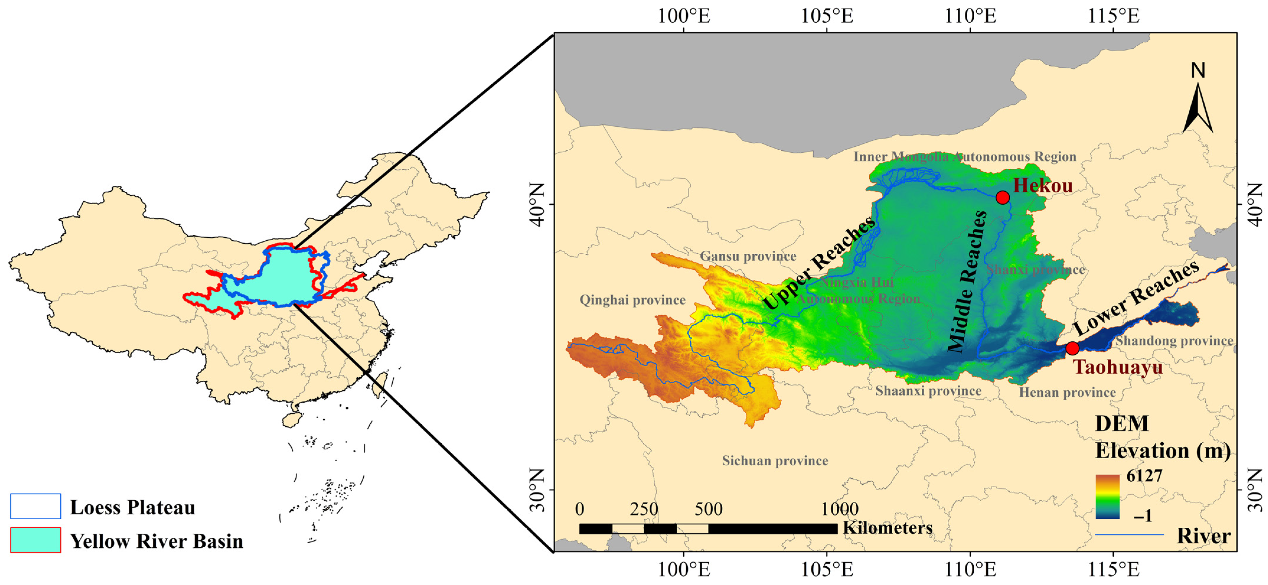
Figure 1. Overview of the YRB.
Remotesensing 17 03967 g001
Figure 2. Research framework. This figure presents a subset of the identified lag and accumulation patterns. Distinct colors denote different categories: white and gray indicate non-computable and non-significant results, respectively; khaki, green, blue, and purple represent conditions of no lag, one-month, two-month, and three-month lags, respectively; while light green, orange, and brown denote one-month, two-month, and three-month accumulation effects, respectively.
Remotesensing 17 03967 g002
Figure 3. Spatial and temporal consistency between harmonized GLASS and MODIS LAI data for the validation sets: (a) Coefficient of determination (R2) between depicting pixel-wise agreement GLASS and MODIS data. (b) Monthly time series of spatially averaged LAI from GLASS and MODIS data.
Remotesensing 17 03967 g003
Figure 4. Comparison between the harmonized LAI dataset and two LAI products (GLOBMAP and GEOV2), including (a) pixel-level scatter plot with GLOBMAP, (b) monthly LAI distribution boxplots for GLOBMAP, (c) pixel-level scatter plot with GEOV2, and (d) monthly LAI distribution boxplots for GEOV2, for consistency assessment.
Remotesensing 17 03967 g004
Figure 5. Spatial distribution of LAI trends and significance test results under the historical period and three future scenarios.
Remotesensing 17 03967 g005
Figure 6. Interannual variability, 5-year moving averages, and linear trends of LAI under the historical period and three future scenarios.
Remotesensing 17 03967 g006
Figure 7. The VIP values of the 26 extreme climate indices under historical and future SSP scenarios (The red and yellow lines denote the VIP = 1 and VIP = 0.8 thresholds used to identify key influencing factors).
Remotesensing 17 03967 g007
Figure 8. Time lag effect of five key indices on vegetation LAI under different scenarios.
Remotesensing 17 03967 g008
Figure 9. Composition of lag month effects for the five indices under the three SSP scenarios (% of pixels).
Remotesensing 17 03967 g009
Figure 10. Cumulative effect of five key indices on vegetation LAI under different scenarios.
Remotesensing 17 03967 g010
Figure 11. Composition of accumulation-month effects for the five indices under three SSP scenarios (% of pixels).
Remotesensing 17 03967 g011
Table 1. Construction and Evaluation of PLSR Models Based on Long-Term Time Series.
ScenarioNumber of ComponentsR2Beta Coefficient
FDGSLSUIDPRCPTOT
SSP2-4.560.805−0.440.120.13−0.16−0.44
SSP3-7.060.805−0.60−0.150.24−0.25−0.24
SSP5−8.560.824−0.670.120.09−0.15−0.36
Disclaimer/Publisher’s Note: The statements, opinions and data contained in all publications are solely those of the individual author(s) and contributor(s) and not of MDPI and/or the editor(s). MDPI and/or the editor(s) disclaim responsibility for any injury to people or property resulting from any ideas, methods, instructions or products referred to in the content.