A 3D GeoHash-Based Geocoding Algorithm for Urban Three-Dimensional Objects

Highlights

What are the main findings?

• A 3D GeoHash-based geocoding algorithm was developed for real-time, lightweight 3D urban modeling.
• The method achieved 9.8× faster performance than orthophoto-based modeling with full object accuracy.

What are the implications of the main findings?

• The 3D GeoHash provides a unified spatial key linking query, visualization, and simulation.
• It establishes a foundation for operational digital twins and predictive disaster management.

Abstract

The growing frequency of extreme weather, earthquakes, fires, and environmental hazards underscores the need for real-time monitoring and predictive management at the urban scale. Conventional three-dimensional spatial information systems, which rely on orthophotos and ground surveys, often suffer from computational inefficiency and data overload when processing large and heterogeneous datasets. To address these limitations, this study introduces a three-dimensional GeoHash-based geocoding algorithm designed for lightweight, real-time, and attribute-driven digital twin operations. The proposed method comprises five integrated steps: generation of 3D GeoHash grids using longitude, latitude, and altitude coordinates; integration with GIS-based urban 3D models; level optimization using the Shape Overlap Ratio (SOR) with a threshold of 0.90; representative object labeling through weighted volume ratios; and altitude correction using DEM interpolation. Validation using a testbed in Sillim-dong, Seoul (10.19 km²), demonstrated that the framework achieved approximately 9.8 times faster 3D modeling performance than conventional orthophoto-based methods, while maintaining complete object recognition accuracy. The results confirm that the 3D GeoHash framework provides a unified spatial key structure that enhances data interoperability across querying, visualization, and simulation. This approach offers a practical foundation for operational digital twins, supporting high-efficiency 3D mapping and predictive disaster management toward resilient and data-driven urban systems.

1. Introduction

1.1. Background and Research Necessity

In recent years, the frequency of urban disasters has been increasing due to extreme climatic events, earthquakes, fires, construction accidents, and air pollution, all of which are intensified by changes in urban and meteorological environments. In Republic of Korea, nine cases of extreme rainfall events exceeding 100 mm h⁻¹ were recorded in 2024, while Typhoon Hinnamnor in 2022 brought a daily maximum precipitation of 342.4 mm and resulted in 11 fatalities. The summer of 2024 (June–August) also marked the highest national average temperature on record (25.6 °C), demonstrating a clear intensification of extreme weather events. Seismic activity has likewise increased, with major earthquakes such as the 2016 Gyeongju (M 5.9) and 2017 Pohang (M 5.4) events, followed by 16 earthquakes above magnitude 3 in 2023 and 7 in 2024, indicating that Korea can no longer be regarded as a seismically safe region. Large-scale disasters caused by fires and construction accidents have also continued to occur, including the 2022 Uljin, 2023 Gangneung, and 2025 Yangyang wildfires (the Uljin fire alone caused an estimated ₩900 billion in damages), as well as the 2025 Busan hotel construction fire (6 fatalities) and 2025 Anseong bridge collapse (4 fatalities). Moreover, fine dust pollution has become so severe that it is officially classified as a social disaster, posing a significant threat to public health. In this context, there is an urgent need for an urban digital twin technology capable of real-time monitoring and predictive management of the increasingly frequent and complex disasters occurring within urban environments.

At present, three-dimensional spatial information is primarily constructed through aerial photography or drone-based orthophotos, combined with drawings, coordinates, and surveying instruments to generate 3D data for all urban objects. However, this approach imposes significant computational and data-processing burdens when handling diverse and large-scale datasets. Conventional disaster simulation methods, such as Computational Fluid Dynamics (CFD) and Moving Particle Simulation (MPS), are also constrained by high computational complexity and resource requirements, limiting their applicability to small-scale sites or specific disaster types. For predictive disaster management at the urban scale, it is therefore essential to develop a property-based, real-time automated digitalization and three-dimensional adaptive mapping technology that enables independent interactions within a virtual space.

To construct a digitalized virtual space in which diverse urban objects and sensors—such as those related to construction, road traffic, meteorological conditions, air quality, and multiple satellite systems—interact with one another, it is necessary to integrate not only fundamental spatial data (e.g., buildings and terrain) but also environmental factors (e.g., weather and air-pollution information) and physical factors (e.g., construction machinery and transportation systems). In this process, remote-sensing imagery, drone-based observations, and GNSS-derived positioning and displacement data can serve as primary data sources. The proposed 3D GeoHash provides an indexing and geocoding layer that acts as a common spatial key to efficiently align and update these heterogeneous observations in real time. Specifically, this study proposes a 3D GeoHash-based virtual spatial-information framework in which spatial grids are fixed while static and dynamic, location-based attributes of urban objects move across those fixed grids. By applying additional sub-division according to spatial characteristics, incorporating material-specific physical properties, and performing coordinate-based real-time geocoding, the proposed method aims to realize an intuitive and lightweight 3D urban-object geocoding system. The primary objective of this study is to validate the operational feasibility of the proposed framework through a test-bed implementation.

1.2. Study Scope and Methodology

As this study aims to support urban monitoring and predictive management, it is necessary to define an appropriate spatial scope at the regional level. Although the basic 3D GeoHash cell structure can theoretically cover the entire globe at level 0, this study defines the Korean Peninsula as the level-0 base region to reflect disaster-simulation applications in Korean cities. The study focuses on real-time urban digital-twin implementation and, further, on the predictive management of urban disasters such as flooding, wildfires, and air pollution. For empirical validation, Sillim-dong in Seoul was selected as the testbed area, as it includes diverse urban and environmental features such as mountains, rivers, and residential and commercial zones.

This research develops and validates a 3D GeoHash-based geocoding algorithm for urban three-dimensional objects. The methodological framework consists of the following five steps. For validation, 3D GeoHash values of major urban objects—such as buildings, roads, mountains, and rivers—are computed and visualized for the Sillim-dong testbed area in Seoul.

(1)

Generation of the 3D GeoHash: Extend the conventional two-dimensional GeoHash by incorporating altitude information, thereby creating a Korean Peninsula-based 3D GeoHash index.

(2)

Integration with GIS Data: Combine the generated 3D GeoHash with urban 3D models derived from GIS datasets such as digital topographic maps and road-name address data.

(3)

Optimization of GeoHash Resolution: Compute the geometric overlap ratio between 3D urban objects and GeoHash cells to determine the optimal GeoHash level.

(4)

Classification of Urban Objects: Calculate volumetric ratios for each object to classify urban-object types within the 3D GeoHash framework.

(5)

3D GeoCoding with Terrain Interpolation: Perform DEM-based 3D GeoHash geocoding using a Terrain-Normalized Interpolation (TNI) method to reflect topographical variations.

1.3. Literature Review

1.3.1. Tree-Dimensional Spatial Information

This study aims to construct a three-dimensional virtual spatial-information framework that incorporates attribute data, enabling digital-twin implementation and simulation. Accordingly, this section reviews previous research on representing urban environments through 3D spatial information. Existing studies on digital-twin-based 3D spatial data can be broadly categorized into (a) research on urban digital twins and (b) research on three-dimensional grids and voxels.

Regarding urban digital-twin research, recent studies have emphasized bidirectional synchronization between the physical and virtual worlds, while identifying standard-based data integration and real-time operability as common challenges—particularly with standards such as CityGML, IFC, 3D Tiles, and IndoorGML [1,2,3,4,5,6,7].

For example, Mazzetto (2024) highlighted that the success of urban digital twins depends critically on the integration of heterogeneous data and low-latency synchronization [1]. Jeddoub et al., (2023) identified the absence of a common spatial unit as the primary factor contributing to the gap between conceptual design and implementation [2]. Therias and Rafiee (2023) discussed the importance of linking simulation models to urban resilience analysis [3]. In terms of standardization, recent advances include the IndoorGML indoor network model, CityGML–IFC integration, and 3D Tiles-based web streaming, which have collectively improved large-scale visualization and interoperability [4,5,6,7].

Meanwhile, research on three-dimensional grid and voxel structures has mainly evolved toward improving numerical analysis and simulation efficiency. Methods such as the Scale-Elastic Grid System (SEGS) and hybrid boundary–voxel models have demonstrated strengths in hierarchically partitioning large-scale urban data while representing occupancy and uncertainty [8,9,10]. Extensions of spatial-indexing structures—including Octree, 3D R-tree/R*-tree, and Morton/Hilbert-based space-filling curves—have proven their effectiveness in accelerating database queries for 3D point clouds and urban models [11,12,13,14]. Furthermore, several studies have utilized 3D volumetric-grid frameworks for applications such as UAV air-route planning, urban-area GPS simulation, coastal-zone management, and fine-dust visualization [15,16,17,18,19].

More recent works have moved beyond volumetric partitioning to focus on spatial-database storage and utilization, introducing models such as the Sphere Shell Space 3D Grid (SSSG) [20], GeoSOT-3D [21], multi-grid spatial-partitioning methods [22], and Discrete Global Grid Systems (DGGS) [23,24,25]. However, these approaches often rely on multiple heterogeneous indexing units (e.g., layers, tiles, object IDs), making it difficult to unify real-time queries, streaming, and simulation calls under a single indexing rule. In addition, voxel-based or traditional 3D index structures impose high costs for updating and rebalancing, rendering them less suitable for online operations and heterogeneous-data joins.

In digital-twin operations, therefore, a lightweight common spatial key that includes the vertical (z-axis) dimension is required. A decoupled architecture—where voxel or Octree structures are used for physical simulations and the common spatial key is used for data indexing and streaming—is particularly desirable. Based on this rationale, the present study adopts a 3D GeoHash-based geocoding framework for urban 3D objects, aiming to optimize both the selection of the appropriate GeoHash level and the representation of urban objects through geometric-overlap and volumetric-ratio labeling.

1.3.2. GeoHash

Research related to 3D GeoHash for simulation can be classified into three categories: GeoAI studies, 2D GeoHash studies, and 3D GeoHash studies.

First, within the field of GeoAI, the conceptual scope and methodologies of spatially explicit artificial intelligence have been established, with increasing sophistication in prediction, detection, and explainability functions [26,27,28,29]. However, many models still rely on two-dimensional or spatially inconsistent units, making it difficult to directly represent vertical contexts such as building heights, terrain variations, and indoor or multilayer environments. Accordingly, there is a growing need for an input framework that unifies learning, inference, and explainability at the level of three-dimensional cells serving as a common spatial key.

GeoHash (2D) originated from Morton’s seminal work in 1966 [30], which introduced a hierarchical spatial data structure that partitions space into grid-shaped buckets. It was later implemented as a public-domain geocoding system invented by Niemeyer in 2008 [31], encoding geographic locations into short alphanumeric strings. More recently, in 2D GeoHash research, approaches such as GeohashTile have been used to optimize vector-data transmission at the code level, while Two-bit Geohash demonstrated high-performance nearest-neighbor and range queries [32]. Other studies have verified code-level level-of-detail (LOD) control, accelerated range and proximity queries, and adaptive-precision streaming [33,34,35]. GeoHash-based spatial analysis has also expanded to mobility applications such as traffic flow and accident prediction [36,37]. Nevertheless, the absence of a vertical (z) dimension limits its applicability in z-sensitive domains—such as wildfire spread, atmospheric phenomena, or multi-story and vertical environments. GeoHash has also been methodologically utilized for visual position estimation for autonomous lunar landings [38].

Finally, 3D GeoHash research has begun to address these limitations. Murugesan et al., (2020) simplified the generation of geohash codes for adjacent grid cells and proposed a two-bit 3D GeoHash encoding algorithm for efficient memory utilization [39]. Lai et al., (2020) introduced a multi-scale integer encoding method supporting basic spatial relationships within 3D grids, applying it to 3D city-model construction [40]. However, practical methodologies that explicitly define geocoding procedures at the urban-object level and integrate them with digital-twin metadata standards remain scarce. Therefore, this study proposes an intuitive and lightweight 3D urban-object geocoding algorithm that generalizes the conventional 2D GeoHash through bit interleaving of latitude, longitude, and altitude, enables additional sub-division based on spatial characteristics, incorporates material-based physical properties, and performs coordinate-based real-time geocoding within a defined 3D spatial domain.

2. Development of the 3D GeoHash-Based Urban Object Geocoding Algorithm

The primary objective of this study is to develop a 3D GeoHash-based geocoding algorithm for three-dimensional urban objects. The algorithm is designed and implemented through the following sequential processes:

(1)

Generation of the 3D GeoHash;

(2)

Integration of the GIS-based 3D urban model with the 3D GeoHash;

(3)

Determination of the optimal 3D GeoHash level;

(4)

Classification of 3D GeoHash urban-object types;

(5)

DEM-based 3D GeoHash geocoding of urban objects.

The process for each step is illustrated in Figure 1.

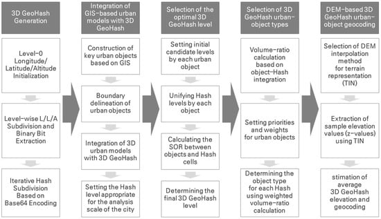
Figure 1. The 3D GeoHash-based urban object geocoding algorithm process.

2.1. Generation of the 3D GeoHash

This study introduces the concept of a 3D GeoHash to enable attribute-based digitalization of urban objects capable of independent interactions within a virtual space. While the conventional GeoHash encodes only two-dimensional coordinates (longitude and latitude), the proposed 3D GeoHash incorporates altitude to encode the triplet (longitude, latitude, altitude). To achieve data compactness suitable for domestic urban-control applications, the initial level (level 0) is defined with reference to the Korean Peninsula. The 3D GeoHash incorporates altitude information using a voxel-based hierarchical spatial structure, subdivided into near-cubic units composed of points, lines, and surfaces to ensure efficient simulation. The generation process proceeds as follows.

2.1.1. Define the Base Cube (Level 0)

The Korean Peninsula is defined as level 0, based on the UTM coordinate system, Zone 52 N. The corresponding longitudinal width (6°) is 526.488 km, the latitudinal height (12°) is 1333.584 km, and the vertical (altitude) range is set to ±250 km.

The altitude extent is chosen to produce a rectangular prism in which the longitudinal width is approximately twice the latitudinal width and the vertical range is half the latitudinal range.

2.1.2. Hierarchical Subdivision

The longitudinal axis is first divided three times, followed by two divisions each along longitude, latitude, and altitude for every level—resulting in six binary digits per level. The initial triple division along longitude compensates for its approximately two-fold scale relative to latitude, producing a near-cubic 3D GeoHash cell structure.

2.1.3. Code Encoding

The obtained binary sequences are converted into Base64 codes, and each newly generated 3D GeoHash code is appended iteratively to the previous hash string to create higher-level 3D GeoHash values. Through this iterative subdivision, the 3D GeoHash values can be generated at any desired resolution level. In this study, to capture centimeter-scale variations in urban-object attributes, 12-level 3D GeoHash codes were generated, corresponding to spatial resolutions of 3.14 cm (latitude), 3.97 cm (longitude), and 2.98 cm (altitude). The final generated 3D GeoHash level sizes are as shown in Table 1.

Table 1. 3D GeoHash level size.

Level	Latitude Size	Longitude Size	Altitude Size	Segmentation	Unit
0	526.488	1333.584	250	-	km
1	131.622	166.698	125	lon-lat-lon-lat-lon-alt	km
2	32.9055	41.6745	31.25	lon-lat-alt-lon-lat-alt	km
3	8.226375	10.418625	7.8125	lon-lat-alt-lon-lat-alt	km
4	2.05659375	2.60465625	1.953125	lon-lat-alt-lon-lat-alt	km
5	0.514148438	0.651164063	0.48828125	lon-lat-alt-lon-lat-alt	km
6	128.5371094	162.7910156	122.0703125	lon-lat-alt-lon-lat-alt	m
7	32.13427734	40.69775391	30.51757813	lon-lat-alt-lon-lat-alt	m
8	8.033569336	10.17443848	7.629394531	lon-lat-alt-lon-lat-alt	m
9	2.008392334	2.543609619	1.907348633	lon-lat-alt-lon-lat-alt	m
10	0.502098083	0.635902405	0.476837158	lon-lat-alt-lon-lat-alt	m
11	12.55245209	15.89756012	11.92092896	lon-lat-alt-lon-lat-alt	cm
12	3.138113022	3.97439003	2.980232239	lon-lat-alt-lon-lat-alt	cm

2.2. Integration of GIS-Based 3D Urban Models with the 3D GeoHash

In this step, the 3D GeoHash grids generated at each level are integrated with GIS-based urban 3D models. The detailed procedure is as follows.

First, major urban objects—such as buildings, roads, rivers, and contour lines—are constructed using a digital topographic map as the base dataset. In Republic of Korea, the Ministry of Land, Infrastructure and Transport provides national digital topographic maps in which terrain features and place names (e.g., roads, buildings, and rivers) are represented as coordinate-based datasets suitable for spatial analysis. These maps, which preserve real-world scale, are available nationwide without spatial restrictions at scales of 1:5000 and 1:25,000.

Second, the boundaries of urban objects are defined through data preprocessing based on the digital topographic map. Although most urban-object boundaries (buildings, roads, rivers, etc.) can be extracted from the topographic data, it is necessary to utilize additional data sources to enhance update frequency and positional accuracy. Since inconsistencies may occur among datasets with different update cycles, the boundaries are aligned based on the most frequently updated dataset, and internal boundaries are merged to prevent duplicate 3D GeoHash generation. In this study, road and river data were obtained from digital topographic maps, administrative boundaries from the Statistics Korea administrative-division dataset, building footprints from the Road Name Address database, and mountain boundaries from the Korea mountaion Spatial Information Service (mountaion type map).

Third, the 3D GeoHash is integrated with these GIS datasets. For each object class (building, road, river, mountaion), the geometric overlap ratio between the object boundary and the GeoHash cell is calculated to determine the optimal 3D GeoHash representation. Customized 3D GeoHash cells are then generated using the object-specific boundary coordinates (x, y) and height information (z). Because height attributes are typically absent from standard GIS datasets, this study derived z-values using attribute information and the digital elevation model (DEM).

Finally, the base 3D GeoHash level is selected according to the monitoring scale. For large-scale regional monitoring, level 6 (latitude: 128.5 m; longitude: 162.8 m; altitude: 122.1 m) is appropriate, whereas for small-scale urban applications, level 7 (latitude: 32.1 m; longitude: 40.7 m; altitude: 30.5 m) provides finer resolution. Given the substantial differences in data volume across levels, it is recommended to begin with a lower GeoHash level and manage individual urban objects in separate layers. The GIS-based city 3D model and 3D GeoHash levels are combined as shown in Figure 2.

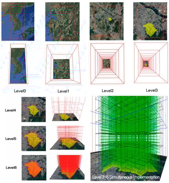
Figure 2. Integration of GIS-based 3D urban models with the 3D GeoHash (Testbed Example, yellow area represents the testbed and green boxes are 3D representations of the GeoHash).

2.3. Determination of the Optimal 3D GeoHash Level

Based on the integrated 3D urban model and the base 3D GeoHash level, this step establishes the optimal 3D GeoHash level for each urban object. The optimization procedure proceeds as follows.

First, the area and shape of each urban object are computed to determine an initial candidate level set. Using the previously defined base level, a first-stage GeoHash level is assigned to each object. For instance, in the case of a building, the object’s geometry is analyzed to calculate its width (W_obj) and height (H_obj), and a candidate GeoHash level is selected such that the grid width (W_grid) and height (H_grid) cover approximately 20% of the object dimensions. The selection condition can be expressed as:

W_grid ≤ W_obj, H_grid ≤ H_obj

(1)

0.8W_obj ≤ W_grid ≤ 1.2W_obj, 0.8H_obj ≤ H_grid ≤ 1.2H_obj (20% range)

(2)

where

• W_obj = object width,
• H_obj = object height,
• W_grid = grid width,
• H_grid = grid height.

Second, the 3D GeoHash levels assigned to the same object are unified. For example, a cubic-shaped building might be assigned Level 8 at its center and Level 9 at its edges. To prevent mixed-level generation, all cells associated with a single object are standardized to the finer level (e.g., if Levels 8 and 9 coexist, Level 9 is adopted).

Third, the Shape Overlap Ratio (SOR) is calculated to quantitatively evaluate the geometric conformity between the voxelized 3D GeoHash and the actual urban-object geometry. SOR is equivalent to the Jaccard coefficient or Intersection-over-Union (IoU) and is defined as:

SOR(G,B) = V(G ∩ B)/(V(G) + V(B) − V(G ∩ B))

(3)

where

• G = voxelized object volume set
• B = reference (actual) building volume set
• V(G) = volume occupied by the grid
• V(B) = volume of the actual building
• V(G ∩ B) = intersection volume between grid and building
• V(G ∪ B) = their union volume.

SOR ranges from 0 to 1, with higher values indicating a more accurate geometric representation of the real object by the 3D GeoHash.

Finally, the upper threshold of SOR is determined to select the final optimal 3D GeoHash level. A higher SOR corresponds to finer subdivision but exponentially increases the number of voxels, resulting in heavier memory requirements. Conversely, an excessively low SOR may distort terrain or building boundaries. Considering the trade-off between voxel growth and approximation error, this study sets the SOR upper limit at 0.90. If the SOR < 0.90, non-building elements such as roads or vegetation may intrude into the same cell, introducing bias and necessitating additional post-processing. When SOR ≥ 0.90, building boundaries are represented continuously, ensuring both topological stability and geometric accuracy—a minimum standard for reliable 3D GeoHash-based urban-object representation. Figure 3 illustrates the shape overlap ratios calculated for different 3D GeoHash levels at the same site.

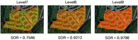
Figure 3. Determination of the optimal 3D GeoHash level for each urban object.

2.4. Classification of 3D GeoHash Urban Object Types

After integrating urban objects with the 3D GeoHash grid, the volume ratio is calculated to determine the representative urban-object type within each 3D GeoHash cell. Let a 3D GeoHash cell be denoted as C, and let the set of urban objects intersecting or contained within the cell be {i = 1, …, N_C}. The volume occupied by object i inside cell C is defined as follows:

$$V_i=A_i\times h_i^{eff}$$

(4)

• $A_i:$ the planar intersection area between cell C and object i
• $h_i^{eff}$: the effective height determined by the intersection of the vertical extents of object i and cell C.

Total volume of all objects within the cell:

$$V_{tot}={\sum }_{j=1}^{N_c}{V}_j$$

(5)

Volume ratio of object i:

$$r_i={\displaystyle \frac{V_i}{V_{tot}}}$$

(6)

Representative urban-object type for cell C:

$$\mathrm{f}\left(\mathrm{C}\right)=\mathrm{a}\mathrm{r}\mathrm{g}\mathrm{m}\mathrm{a}\mathrm{x}\_\left\{\mathrm{i}\in \left\{1,\dots ,{\mathrm{N}}_{\mathrm{C}}\right\}\right\}{r}_i$$

(7)

However, selecting urban-object types solely based on volume ratio may overlook semantically important objects in real urban environments. For example, in a fire simulation, a building may occupy a smaller volume than surrounding air or road space within a given 3D GeoHash cell, yet it remains the most critical feature for assessing fire propagation. Therefore, this study applies a priority-based weighting scheme to better reflect the relative importance of urban objects in disaster and hazard simulations. The priorities and weights of urban objects are as shown in Table 2.

Table 2. Urban object priority and base weights.

Urban Object Type	Priority	Weight (wi)	Rationale
Building	1	1.00	Core element for human and property loss assessment
Bridge	2	0.90	Critical infrastructure; high collapse vulnerability
Road	3	0.70	Essential for rescue, logistics, and firefighting access
Mountain	4	0.50	High risk of wildfire and landslides
River	5	0.50	Prone to flooding and overflow impacts
Air (Empty cell)	6	0.10	Non-physical or unoccupied space

These weights serve as initial coefficients that can be adjusted according to specific simulation scenarios (e.g., flood, fire, or air-pollution models). The weighted volume ratio for each object type is computed as:

$$r_i^{*}={\displaystyle \frac{w_i·V_i}{\sum _{j=1}^{N_c}{w}_j·V_j}}$$

(8)

where $w_i$ is the assigned weight of urban-object type i. The representative urban-object type for cell C is ultimately determined by the object with the maximum weighted volume ratio $r_i^{*}$.

2.5. DEM-Based 3D GeoHash Urban Object Geocoding

This final step involves generating a Digital Elevation Model (DEM) from contour data obtained from a 1:5000-scale digital topographic map and using it to geocode 3D GeoHash urban objects by incorporating terrain elevation. For DEM construction, this study employs the Triangulated Irregular Network (TIN) interpolation method, which is particularly effective for representing linear elevation structures. The TIN approach models continuous terrain surfaces by spatially connecting elevation data points through an irregular network of triangles. It enables the direct use of contour-line vertices as triangle nodes, thereby naturally preserving the linear structure of topographic elevation data. The TIN-based DEM creation process is as shown in Figure 4.

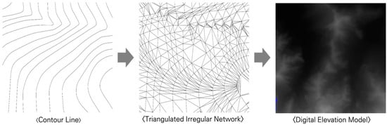
Figure 4. TIN-based DEM creation process.

Since primary urban objects are represented as two-dimensional datasets lacking explicit height information, the DEM was used to extract their elevation (z) values to better reflect the actual terrain. The height extraction was performed after the generation of 3D GeoHash cells for each object, using the mean-elevation estimation method based on the pixel centers of the DEM. This method estimates the representative elevation of a 3D GeoHash cell by averaging the elevation values of DEM pixels whose centers fall within the horizontal projection (rectangular or polygonal footprint) of the GeoHash cell. The method for selecting the center of pixels that fall within the horizontal projection (rectangular area) of 3D GeoHash as samples is as follows.

$$S_{ctr}\left(C\right)=\left(i,j\right)\left|\right(x_i,y_j)\in C$$

(9)

Here, the horizontal projection (rectangular or polygonal area) of the 3D GeoHash is C, and the DEM pixel centers are $(x_i,y_j)$.

The following formula estimates the average elevation of a GeoHash by averaging the elevation values of the samples.

$$\overline{z}\left(C\right)={\displaystyle \frac{1}{\left|S_{ctr}\right(C\left)\right|}}{\sum }_{(i,j)\in S_{ctr}\left(C\right)}{z}_{i,j}$$

(10)

$\overline{z}\left(C\right)$ represents the representative elevation (average elevation) of the horizontal projection (rectangular or polygonal area) of the GeoHash, $z_{i,j}$ represents the elevation value of the pixel centers in the DEM, and ${|S}_{ctr}\left(C\right)|$ represents the number of pixel centers within the voxel.

This approach ensures that the elevation of each GeoHash cell accurately reflects local terrain variations. The extracted height information (z-values) for key urban objects was subsequently used as an essential input parameter for constructing the 3D GeoHash-based urban-object models, thereby determining the vertical positioning of each urban object within the 3D geocoding framework.

3. Development of the 3D GeoHash Data Model

3.1. 3D GeoHash Data Model Framework

This section presents the data-model framework required to implement the proposed 3D GeoHash–based urban-object geocoding algorithm. The voxelized data are stored in the GeoPackage (.gpkg) format, which enables multi-layer storage, metadata embedding, and styling within a single file. This format is well suited for generating spatial indexes in both 2D and 3D (z-dimension).

The data model consists of five primary tables: (i) 3D GeoHash Background, (ii) Urban Object, (iii) 3D GeoHash by Object, (iv) Attribute Information, and (v) Interaction. The entire data model framework of 3D GeoHash is shown in Table 3.

Table 3. The data model framework.

Table Name	Field Name	Data Type	Contents	Notes
3D GeoHash Background	geohash_ID	VAR(255)	3D Geohash unique ID	PK (Fixed ID)
	geohash_code	VAR(255)	geohash code	Position Determination Calculation
	elev_bottom	INT	geohash height value(bottom surface)
	elev_top	INT	geohash height value (top surface)
	geohash_floor	INT	geohash floor information
	metadata	INT, JSON	metadata information
	geohash_level	VAR(255)	geohash generation level
Urban Object	U_object_ID	VAR(255)	urban object ID	PK (Fixed ID)
	build_nm	VAR(255)	building name
	build_height	VAR(255)	height information
	build_floor	VAR(255)	floor count
	build_material	VAR(255)	material
	road_nm	VAR(255)	road name
	road_material	VAR(255)	material
	bridge_nm	VAR(255)	bridge name
	bridge_material	VAR(255)	material
	mount_nm	VAR(255)	mountain name
	mount_material	VAR(255)	material
	river_nm	VAR(255)	river name
	river_material	VAR(255)	material
3D GeoHash by Object	geohash_ft_ID	VAR(255)	geohash feature ID by object	PK (Fixed ID)
	geohash_ID	VAR(255)	geohash unique ID by object	FK (Linked ID)
	U_object_ID	VAR(255)	urban object ID	FK (Linked ID)
	geohash_code	VAR(255)	geohash code	FK (Linked ID)
	object_level	VAR(255)	geohash optimal level by object	Optimal Level Calculation
	object_type	VAR(255)	urban object type	Volume Ratio Calculation
	geohash_Code	VAR(255)	geohash code
	elev_bottom	INT	geohash height value (bottom surface)
	elev_top	INT	geohash height value (top surface)
	geohash_floor	INT	geohash floor information
	geohash_level	VAR(255)	geohash generation level	Generation Level Calculation
Attribute Information	attribute_ID	VAR(255)	attribute unique ID	PK (Fixed ID)
	geohash_ID	VAR(255)	geohash ID	FK (Linked ID)
	geohash_ft_ID	VAR(255)	geohash feature ID by object	FK (Linked ID)
	interaction_ID	VAR(255)	interaction ID	FK (Linked ID)
	attribute_key_r	VAR(255)	primary attribute name
	attribute_key_n	VAR(255)	Nth attribute name
	attribute_level	VAR(255)	attribute level
Interaction	interaction_ID	VAR(255)	interaction ID	PK (Fixed ID)
	property_ID	VAR(255)	physical property ID ID	PK (Fixed ID)
	attribute_ID	VAR(255)	attribute unique ID	FK (Linked ID)
	neighbor_geohash_ID	VAR(255)	neighbor geohash ID	FK (Linked ID)
	neighbor_geohash_ID_n	VAR(255)	Nth neighbor geohash ID
	interaction_type	VAR(255)	interaction type	Interaction Calculation
	property_key	VAR(255)	physical property name
	property_val_b	VAR(255)	original physical property value
	property_val_a	VAR(255)	post-analysis physical property value

First, the 3D GeoHash Background table stores the initial GeoHash information prior to integration with the GIS-based 3D urban model. It includes the positional identification code for each GeoHash cell, level-specific height values, and associated metadata.

Second, the Urban Object table contains GIS and administrative information for major urban objects such as buildings, roads, bridges, forests, and rivers. It includes object-specific attributes such as building names, material types, number of floors (for buildings), and other semantic data.

Third, the 3D GeoHash by Object table represents feature information for each GeoHash cell after integrating the GeoHash structure with urban objects. This table stores the Shape Overlap Ratio (SOR) for determining the optimal GeoHash level, as well as the volume ratio and weighted volume ratio used to assign representative urban-object types.

Fourth, the Attribute Information table contains detailed semantic and physical properties of each cell—such as material characteristics, constituent substances, and attribute levels—derived from interaction-based computations.

Finally, the Interaction table represents physical interactions between adjacent GeoHash cells. It includes physical property values, interaction computation types, and pre-/post-analysis material-property updates.

3.2. 3D GeoHash Data Model Linking Architecture

Based on the previously defined 3D GeoHash data model, a linking and interaction architecture was designed to show how the individual tables are connected. The process begins by integrating the initially generated 3D GeoHash Background table with the GIS-based Urban Object table to construct the 3D GeoHash by Object table. This table computes the positional identification of each GeoHash cell, the optimal GeoHash level using the Shape Overlap Ratio (SOR), and the representative urban-object type using the volume-ratio calculation, thereby producing the “GeoHash Feature ID by Object.”

The resulting GeoHash Feature ID by Object is directly linked to the Attribute Information table. Within this table, the attribute unique ID manages semantic and physical properties of each GeoHash cell, including materials and constituent substances. The Interaction table operates by calculating physical interactions between adjacent GeoHash cells using the cell’s material properties. The computed interaction outcomes—such as updated physical-property values—are then fed back into the Attribute Information table, forming a bidirectional linkage that supports dynamic property updates across the 3D GeoHash structure. Figure 5 shows the 3D GeoHash data model linking architecture.

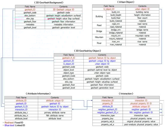
Figure 5. 3D GeoHash Data Model Linking Architecture.

4. Empirical Validation by Urban Object Type

In this section, the 3D GeoHash-based urban-object geocoding algorithm developed in the previous chapters is empirically validated. The process involves computing and visualizing 3D GeoHash values for major urban objects within the designated testbed area.

4.1. Selection of the Testbed Area

For regional-scale urban monitoring and disaster-management applications, the testbed of this study was set to Sillim-dong, Seoul, covering an area of approximately 10.19 km². This area was selected because it encompasses a diverse range of urban and environmental features—including residential, commercial, and business zones, as well as mountainous terrain, river systems, and flood-prone urban areas—which collectively allow for integrated testing of various disaster and hazard simulation scenarios considered in this study. The location of the test bed is shown in Figure 6.

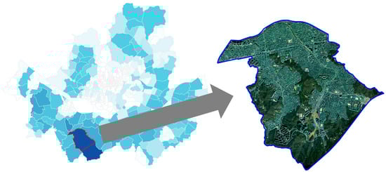
Figure 6. Test-Bed (Sillim-dong, Seoul) (Left: Flood map, The darker the color, the more flooded the area).

4.2. Collection of GIS Base Data

For generating the 3D GeoHash framework of the testbed area, GIS base data were collected for key urban objects—buildings, roads, mountains, and rivers—along with contour data for DEM generation and administrative boundary data. The primary data source was the digital topographic map (scale 1:5000) provided by the National Spatial Information Platform of the Ministry of Land, Infrastructure and Transport. However, to enhance data currency and the accuracy of urban-object boundaries, supplementary datasets were incorporated: building and building-complex data from the Road Name Address Database and mountaion stand maps from the Korea Mountaion Spatial Information Service (FSIS). These datasets together ensured comprehensive coverage and high spatial fidelity for 3D GeoHash generation. The details of the collected datasets—including their sources, coordinate systems, and map scales—are summarized in Table 4 below.

Table 4. GIS basic data collection information.

Object	Dataset/Source	Data Used/Type	Coordinate System	Data Year
building	Road Name Address Database (Address-Based Industry Service)	building/Polygon	EPSG:5179	08.2025
building-complex	Road Name Address Database (Address-Based Industry Service)	building-complex/Polygon		08.2025
Road	Digital Topographic Map (National Spatial Information Platform)	Road Boundary/Polygon		04.2025
Mountain	Mountain Type Map (Korea Mountain Spatial Information Service)	Mountain Stand/Polygon		12.2024
River	Digital Topographic Map (National Spatial Information Platform)	River Boundary/Polygon		04.2025
Administrative Boundary	Census Administrative-Dong Boundary (V-World)	Administrative Boundary/Polygon	EPSG:5186	12.2024
Contour Lines	Digital Topographic Map (National Spatial Information Platform)	Contour/Line	EPSG:5179	04.2025

For buildings, both individual building objects and building complexes of similar use within the same area were classified under a new categorization scheme. This classification was necessary because small-scale residential buildings and apartment complexes with narrow inter-building spacing could otherwise be misinterpreted as overlapping objects or empty spaces during 3D GeoHash generation. The dataset employed for this process was the Building Complex Data provided in the Road Name Address Database. The 3D GeoHash for each building complex was generated based on the number of floors of the tallest building within the complex, which served as the reference height criterion. An example of 3D GeoHash generation for a building complex is shown in Figure 7.

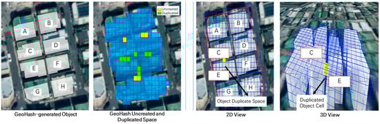
Figure 7. Example of 3D GeoHash generation for a building complex.

For roads, the road-boundary data from the Digital Topographic Map were utilized. Because the road boundaries in the digital topographic dataset are divided into individual segments—such as road connections and intersections—the internal segments were merged to construct a continuous road-boundary dataset. For bridges, the bridge data from the same digital topographic source were used. Since the bridge dataset is spatially continuous with the road boundaries, the overlapping portions between bridges and roads were retained and integrated to preserve topological consistency.

The mountaion boundaries were defined using the Mountaion Type Map provided by the Korea Mountain Spatial Information Service, which is compiled and updated annually by the Korea Mountain Service. This dataset was used to accurately delineate forested areas within the testbed. For rivers, annually updated river-boundary data from the Digital Topographic Map were employed. Because this dataset defines the river boundary rather than only the centerline, it was well suited for GIS-based implementation without requiring additional spatial correction. The air (atmospheric space) was treated as an empty volume without a separate GIS dataset. However, the system is designed so that, in future work, attribute information and physical properties can be assigned to this empty space to enable volumetric modeling of atmospheric phenomena. GIS data for roads (including bridges), mountains, and rivers are shown in Figure 8.

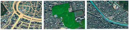
Figure 8. GIS data for roads (including bridges), mountains, and rivers.

4.3. Generation of the 3D GeoHash for the Testbed

For the testbed area of Sillim-dong, Seoul, the base 3D GeoHash level was set to Level 6, corresponding to spatial resolutions of 128.5 m (latitude), 162.8 m (longitude), and 122.1 m (altitude). This level was selected considering the maximum elevation of the surrounding mountains (375 m) and the vertical range represented in the DEM (15–375 m). At Level 6, the vertical domain of Level 5 (approximately 488.3 m) can be subdivided into four hierarchical layers, adequately encompassing the elevation range of the testbed terrain. The chosen latitude and longitude resolutions also provide an appropriate spatial scale for urban-scale disaster analysis, particularly for simulation scenarios such as urban flooding and wildfire propagation. Based on this configuration, the upper-level 3D GeoHash cells were generated for the major urban objects—including buildings, roads, mountains, and rivers—within the testbed area. Figure 9 shows the 3D GeoHash generation based on the testbed target level 6.

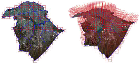
Figure 9. Test-bed 3D GeoHash Generation ((Left): 2D, (Right): 3D; Blue indicates detailed administrative boundaries, and red indicates 3D GeoHash).

According to the previously developed algorithm for determining the optimal 3D GeoHash level, the results for each urban object type were as follows: buildings (Level 8), building complexes (Level 8), roads (Level 9), bridges (Level 9), and mountains and rivers (Level 9). For buildings, the floor height was set to 2.5 m per story, based on the Korean Housing Act (minimum 2.4 m) and the standard floor-height range commonly used in construction; certain high-rise buildings were assigned 3.5 m per story. At Level 8, this produced 187,160 building 3D GeoHash objects, totaling 191.4 MB in size. For building complexes, the number of floors in the tallest building within each complex was used to generate the 3D GeoHash, also applying the 2.5 m per-story height. The resulting number of objects was 10,283, with a total data size of 10.8 MB. For roads, a single 3D GeoHash layer was generated at ground level, resulting in 385,072 objects with a total size of 401 MB. Bridges were generated similarly, producing 5591 objects with a total size of 5.93 MB. For mountains and rivers, one ground-level 3D GeoHash layer was also generated, yielding 85,423 mountain objects (89.1 MB) and 19,173 river objects (20.0 MB), respectively.

To further reduce data volume after the initial generation of 3D GeoHash cells for each urban object type, a cluster-based merging process was applied. In this procedure, adjacent GeoHash cells belonging to the same object and sharing identical attribute information were merged into a single cluster.

For buildings, the original 187,160 GeoHash cells (191.4 MB) were reduced to 7753 cells (42.3 MB), achieving substantial compression—approximately a 96% reduction in cell count and a 78% reduction in data size. Road features were also merged by combining all contiguous segments into single Hash units, reducing the data volume from 401.0 MB to 145.4 MB (36.3% of the original). For bridges, cluster merging reduced the number of GeoHash cells from 5591 (5.93 MB) to 24 cells (1.1 MB), corresponding to 18.5% of the original data size. In the case of forests, the number of GeoHash cells decreased from 85,423 (89.1 MB) to 11 clusters (40.7 MB), and for rivers, from 19,173 cells (20.0 MB) to 13 clusters (4.2 MB), achieving data-size reductions to 45.7% and 21.0% of the originals, respectively.

These compression results demonstrate a significant improvement in storage efficiency and are expected to substantially enhance performance in computation, visualization, and simulation processes by enabling object-level operations on lighter datasets. Figure 10 shows the city object merged into the cluster after the first generation of 3D GeoHash.

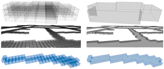
Figure 10. Cluster Merge (Building, Road, River).

The ground-elevation reference for each object was established based on the corresponding DEM-derived elevation values, adjusted to account for object-specific characteristics. For buildings and building complexes, the average DEM value across all GeoHash cells composing each object was used as the ground-elevation reference. For instance, if a single building was represented by six GeoHash cells, the mean of the six DEM elevations was applied as its base height, reflecting the assumption of construction on a relatively level foundation. In the case of roads, bridges, mountains, and rivers, the DEM values at each GeoHash cell were directly used to define ground elevation. This approach allows for more realistic representation of vertical conditions and facilitates integration with simulation models that require accurate terrain-based height parameters.

For future high-fidelity simulations, we plan to assign differentiated height values to individual urban objects (e.g., building-level height variations) based on additional administrative and cadastral information. To accommodate such updates, the system has been modularized so that any changes in altitude reference automatically trigger the corresponding adjustment of the 3D GeoHash structure. The 3D GeoHash test-bed generation values are shown in Table 5.

Table 5. 3D GeoHash Test-bed Generation Values.

Object	Level	1st Generation		Merge a Cluster		Elevation Reference	Ground Elevation Reference
		Number of Cells	Data Size	Number of Cells	Data Size
building	8	187,160	191.4 MB	7753	42.3 MB	Number of stories × 2.5 m	Mean DEM value of object GeoHashes
building-complex	8	10,283	10.8 MB	1	0.9 MB	Tallest building stories × 2.5 m
Road	9	385,072	401 MB	1	145.4 MB	One ground layer (1.9 m)	DEM value per object GeoHash
Bridge	9	5591	5.93 MB	24	1.1 MB	One ground layer (1.9 m)
Mountain	9	85,423	89.1 MB	11	40.7 MB	One ground layer (1.9 m)
River	9	19,173	20.0 MB	13	4.2 MB	One sub-ground layer (1.9 m)

4.4. Visualization of 3D GeoHash Urban Objects

For visualization of the 3D GeoHash results for each urban object, the open-source GIS software QGIS (v3.40 LTR) was employed. QGIS is widely used for spatial data analysis and is particularly effective in processing and displaying spatial datasets such as digital topographic maps and road name address data. It provides a 3D View function that enables efficient rendering and analysis of 3D GeoHash-based spatial models; this feature was utilized for visualization in this study. For buildings, the 3D GeoHash visualization results are shown as vertically stacked levels corresponding to building heights, meaning that the height of each object varies according to its number of floors. In contrast, building complexes were visualized using the height of the tallest building within each complex as the reference value, resulting in uniform GeoHash heights across the entire complex. Figure 11 is a 3D GeoHash visualization of the ground and basement floors of the test bed target building.

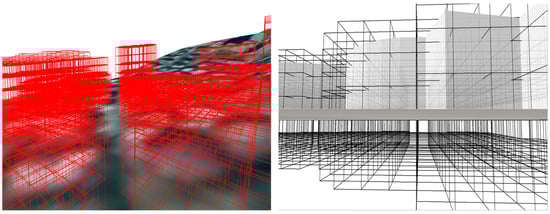
Figure 11. Testbed building visualization.

Despite generating the 3D GeoHash using DEM-based elevation data, certain urban objects failed to fully reflect terrain height variations during visualization. To address this issue, a method of reducing the pixel resolution of the visualization map tiles was applied. Although this approach leads to lower visual sharpness and reduced terrain detail in the rendered output, it has the advantage of accurately preserving the actual DEM elevation values during visualization. From the perspective of enhancing the realism and fidelity of simulation results—one of the primary objectives of this study—the adjustment of map-tile resolution was found to be an effective and practical approach for improving terrain-based rendering consistency. Figure 12 illustrates the reflection of DEM elevation values achieved by adjusting the map-tile resolution.

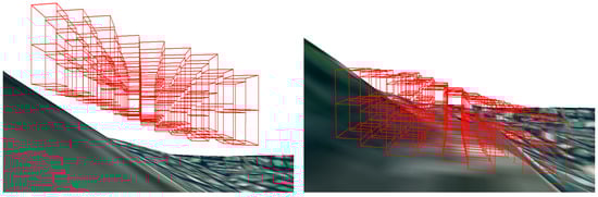
Figure 12. Visualization Reflecting DEM Elevation Values.

For roads and bridges, only a single ground-level layer of 3D GeoHash was generated according to each level. The ground elevation reference for each GeoHash cell was assigned by calculating the mean surface height from the DEM corresponding to the area covered by that cell. To ensure accurate visualization in sloped or uneven terrains, individual ground-elevation values derived from the DEM were applied to each 3D GeoHash cell, allowing realistic alignment of road and bridge surfaces with the underlying topography. Figure 13 shows a 3D GeoHash visualization of roads and bridges.

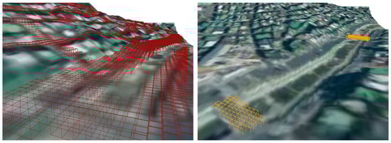
Figure 13. 3D GeoHash visualization of roads and bridges.

In the generation of 3D GeoHash for mountains and rivers, the ground elevation of each GeoHash cell was calculated using the mean DEM value, in the same manner as for other object types. For mountains, a single ground-level layer was generated on the surface at each level, similar to the configuration used for roads and bridges. However, for rivers, a single sub-ground layer of 3D GeoHash was generated below the ground elevation, corresponding to one level size beneath the DEM-derived surface height. Figure 14 shows a 3D GeoHash representation of mountains and rivers. And Figure 15 shows a visualization of a portion of the testbed area containing various urban objects.

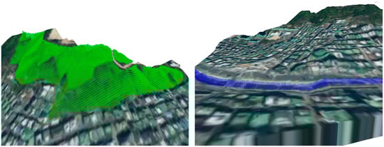
Figure 14. 3D GeoHash visualization of mountains and rivers.

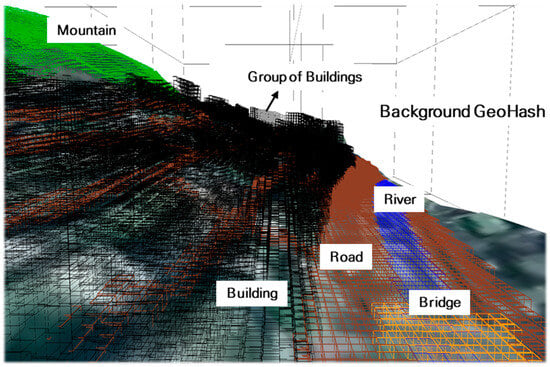
Figure 15. 3D GeoHash visualization of various city objects.

4.5. Performance Test of 3D GeoHash Processing Speed

This section evaluates the computational performance of the developed 3D GeoHash algorithm for 3D model generation, in order to assess its potential for future real-time digital twin applications. The test compares the 3D generation speed of the proposed 3D GeoHash method with that of orthophoto-based 3D modeling. The conventional orthophoto-based 3D modeling workflow consists of extracting building objects from orthophoto digitization, followed by computing floor counts and height information for each building (excluding the manual digitization). In contrast, the 3D GeoHash-based modeling refers to the process of generating predefined voxel-type 3D GeoHash models for building objects within the same test site. To ensure the reliability of the comparison, both tests were conducted under identical experimental and computational conditions. The system specifications included an 11th-generation Intel(R) Core(TM) i5-11400F CPU (at 2.60 GHz), 64 GB of RAM, and a 1.38 TB hard drive. The same orthophoto image of the test site, covering an area of 596.0 m × 437.3 m, was used for all experiments.

Orthophoto-based 3D modeling was performed by first conducting manual digitization of the orthophotos, followed by 3D conversion of the digitized features, floor-count computation, per-floor 3D geometry generation, and attribute assignment (height information). Excluding the manual digitization step, the subsequent 3D data-generation process modeled a total of 352 buildings in 154.1 s, corresponding to a processing rate of approximately 2.3 buildings per second.

For the 3D GeoHash-based modeling, the proposed algorithm was implemented as dedicated software named GeoHash 3D Generator (v1). By simply uploading the same building dataset, 3D GeoHash models were generated through an automated process. To achieve a spatial resolution comparable to that of the orthophoto-based model, the GeoHash level was set to Level 9 (2.0 × 2.5 × 1.9 m). The resulting processing time for generating 352 buildings was 15.7 s, equivalent to 22.42 buildings per second, which is approximately 9.8 times faster than the orthophoto-based approach.

This comparison focused solely on the 3D object generation stage. If the time required for the manual digitization in the orthophoto-based workflow were included, the total computational gap would be even greater. Table 6 and Figure 16 show the performance comparison results for the two comparison groups.

Table 6. Performance test of 3D GeoHash processing speed.

Category	Orthophoto-Based Conventional 3D Modeling		3D GeoHash-Based 3D Modeling
	Workflow Step	Time (s)	Workflow Step	Time (s)
2D → 3D Conversion	3D conversion of digitized data	16.2	3D GeoHash generation	15.7
3D Modeling	Floor-count computation	27.3
	Per-floor 3D geometry generation	87.5
	Attribute assignment	23.1
Total 3D-model generation		154.1	Total	15.7
Objects generated per second		2.3	Objects generated per second	22.4 (13.9× faster performance)

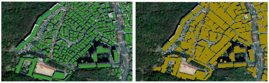
Figure 16. 3D modeling generation performance comparison results ((left): conventional method, (right): 3D GeoHash).

5. Discussion

5.1. Originality Compared with Conventional Digital-Twin 3D Modeling Approaches

This study presented a lightweight 3D GeoHash–based spatial framework designed to support real-time urban digital twin operations and, further, the predictive management of urban hazards such as flooding, wildfires, and air pollution. To assess the practical utility and commercialization potential of the proposed approach, it is essential to compare it with existing 3D digital-twin modeling workflows and clarify the originality and distinctions of the method.

According to the National Geographic Information Institute (NGII) of Korea, current 3D spatial-information production methods consist of the following steps.

First, aerial photography is conducted with sufficient overlap in both north–south and east–west directions to generate realistic orthophotos and 3D visualization models.

Second, airborne LiDAR surveying collects dense elevation measurements by mounting a LiDAR sensor on an aircraft to produce high-accuracy digital elevation models (DEMs).

Third, 3D visualization models of structures such as buildings are generated using aerial imagery and DEMs to reproduce realistic geometric forms.

Fourth, true orthophoto generation removes all geometric distortions of terrain and structure features using DEMs and 3D visualization models.

Finally, 3D spatial-information construction is performed using automated image-matching software to derive true orthophotos, digital surface models, and 3D visualization models [41].

Although these conventional 3D spatial-information production workflows rely heavily on aerial photographs, LiDAR, and satellite imagery, they require substantial manual processing throughout modeling and texturing. Such manual operations result in long production times and increased labor costs, making the approach less efficient in terms of productivity and economics. Nonetheless, because visualization is the primary purpose of traditional 3D modeling, these approaches offer the advantage of achieving high-level realism, with flexible Level-of-Detail (LOD) representations that closely resemble real-world appearances.

In contrast, the objective of the present study is not high-fidelity visualization but the real-time representation of urban activities and ultra-short-term prediction. For these purposes, a more intuitive and lightweight spatial model is necessary. Applying conventional 3D modeling approaches at the entire-city scale requires processing extremely large data volumes, which makes real-time updates and prediction computationally impractical. This limitation motivates the use of 3D GeoHash, which—although less visually realistic—supports independent voxel-level interactions and real-time, attribute-driven automatic digitalization in a virtual environment.

A key advantage of the proposed framework is its scalability, enabling representation not only at the macro urban scale but also at finer micro-scale resolutions through adjustable GeoHash levels. For example, although levels 8–9 were used in this study to support city-scale analysis, levels 11–12 (with cell sizes on the order of centimeters) can be employed for detailed analysis of small-scale facilities, logistics objects, or local operational environments. Therefore, the proposed 3D GeoHash–based framework provides significant benefits in terms of efficiency, practicality, and extensibility, supporting both city-scale real-time digital twin operations and micro-level analytical applications within a unified spatial structure.

5.2. Interaction Mechanism Between Hash Cells

For the proposed framework to be practically deployable, physical state changes derived from interactions between neighboring Hash cells must be computed and reflected in the urban digital twin based on each cell’s object type and attribute information. In this study, the Interaction table was designed within the 3D GeoHash data-model architecture (Section 3) to enable material-property–based interaction analysis and bidirectional linkage among adjacent Hash cells. However, this table provides only a conceptual framework; substantial additional work is required to operationalize inter-Hash interactions.

First, a classification scheme for urban objects must be established for 3D GeoHash generation. Whereas conventional digital twins primarily model fixed GIS-based objects such as buildings, roads, terrain, and rivers, the proposed approach can incorporate not only fixed spatial information but also dynamic phenomena such as weather conditions, fire spread, and moving agents at the resolution of individual Hash cells. Atmospheric Hash attributes include temperature, humidity, precipitation, wind direction, wind speed, and air pollutants (e.g., PM_2.5), which can be updated in real time through Korea Meteorological Administration APIs. Fire-related data can be categorized into types such as ordinary combustibles, flammable liquids, electrical fires, and gas fires, supported by Korea Forest Service datasets or dummy inputs for simulation. Moving-object information—including pedestrians, vehicles, and construction machinery—can be integrated through object detection using CCTV feeds from urban control centers.

Second, object-specific attributes and material properties must be defined. For example, buildings may use concrete as an attribute, while unit weight, compressive strength, and elastic modulus serve as material properties. Since even a single material category (e.g., concrete) may contain dozens of physical parameters, a representative subset must be selected according to the simulation purpose. In fire simulations, for instance, building unit weight and thermal expansion coefficients must interact with atmospheric attributes such as temperature, humidity, wind speed, and wind direction to compute fire propagation.

Third, a movement framework between Hash cells must be constructed. Fixed spatial information—buildings, roads, and terrain—forms “static Hash cells” that cannot move across cell boundaries, whereas dynamic spatial information—air, fire, and moving agents—forms “dynamic Hash cells” that can freely transition to adjacent cells. Across major simulation scenarios, fire, floodwater, and air pollution can all propagate between cells. However, unlike fire—which interacts with fixed environmental elements (e.g., buildings or forests) during its spread—floodwater and air pollutants cannot merge with fixed spatial objects and therefore detour around them, propagating through adjacent open cells instead.

Fourth, interoperability with existing simulators is essential. The primary strength of the proposed system is its ability to support lightweight real-time, city-scale digital-twin operations. Although inter-Hash interaction analysis is feasible, achieving the full accuracy and granularity of established disaster simulators is impractical. Therefore, 3D GeoHash should interoperate with standard data models such as CityGML to ensure extensibility, and should connect with existing simulators. A hybrid workflow—linking 3D GeoHash with tools such as the Fire Dynamics Simulator (FDS) or urban hydrodynamic and flood models—would allow simulator outputs to be mapped onto the Hash cells and subsequently updated through lightweight real-time predictive adjustments. Large-scale simulators typically cannot achieve real-time performance due to the computational burden of processing massive datasets, which underscores the necessity of a 3D GeoHash–based short-term (near–real-time) digital twin. Rather than fully replicating complex physical models within 3D GeoHash, it is more efficient and practical to maintain a lightweight, observation-driven real-time simulation structure augmented by external simulator outputs.

Going forward, continued research on inter-Hash interaction analysis will be essential to extend this framework into a foundational platform capable of supporting both live digital twins—capable of real-time representation of diverse urban activities for city operations—and ultra-short-term predictive analytics for disaster scenarios.

6. Conclusions

This study aimed to develop a real-time urban monitoring and prediction framework by designing and implementing a latitude–longitude–altitude–based 3D GeoHash system and proposing a corresponding three-dimensional urban object geocoding algorithm. The algorithm was structured into five main stages:

(i)

Generation of a 3D GeoHash based on the Korean Peninsula as the level-0 reference;

(ii)

Integration of GIS-based urban 3D models with the 3D GeoHash grid;

(iii)

Determination of the optimal level using the Shape Overlap Ratio (SOR) with an upper threshold of 0.90;

(iv)

Labeling of representative objects based on a volume-ratio and priority-weighting method;

(v)

Altitude correction using DEM (TIN) interpolation.

The proposed algorithm was applied to a testbed in Sillim-dong, Seoul (approximately 10.19 km²). When level 6 was set as the base and major urban objects—including buildings, roads, bridges, mountains, and rivers—were subdivided mainly into levels 8–9, the following results were obtained: 187,160 building objects (191.4 MB) and 10,283 building-group objects (10.8 MB) at level 8, and 385,072 road objects (401 MB), 5591 bridges (5.93 MB), 85,423 mountain grids (89.1 MB), and 19,173 river grids (20.0 MB) at level 9. To achieve further data reduction, a cluster-based merging procedure was applied, which resulted in an additional reduction in data volume by up to approximately 80%.

The framework unified the functional hierarchy of code level (ℓ) = Level of Detail (LOD), ensuring consistency among querying, transmission, visualization, and simulation operations within a common key space. The SOR ≥ 0.90 criterion was demonstrated to be a practical equilibrium between boundary-topology stability and the trade-off of data storage and computational cost. Furthermore, the incorporation of disaster-impact priorities—building > bridge > road > mountain > river > air—into the volume-ratio-based classification enhanced both categorical consistency and contextual relevance for disaster-response scenarios.

Experimental validation confirmed that the proposed 3D GeoHash method achieved approximately 13.9 times higher computational performance than conventional orthophoto-based 3D modeling. This significant improvement suggests strong potential for high-efficiency visualization of large-scale datasets, sustainable 3D mapping, and multi-purpose simulations for disaster and environmental assessments. Overall, the proposed framework establishes a foundation for an operational digital twin, capable of linking streaming, querying, and simulation processes through a unified 3D GeoHash key. It demonstrates the feasibility of a lightweight, variable-resolution, and scalable geospatial geocoding architecture, contributing to the realization of next-generation, data-driven, and resilient urban digital twins.

The limitations of this study are as follows. First, standardized comparison and performance benchmarking were limited. Systematic metadata mapping and interoperability benchmarking with global standards such as H3/DGGS, 3D Tiles Next, and CityGML/IndoorGML were not fully conducted. Second, terrain and boundary consistency were found to be sensitive to the resolution and update frequency of the DEM. In addition, rendering artifacts that appeared during visualization—caused by map tile resolution adjustments—require separate optimization for real-time operational performance. Third, the SOR threshold (0.90) and level-selection criteria were derived empirically from the Sillim-dong testbed; therefore, further research is needed to determine adaptive threshold values for different urban morphologies, densities, and disaster types. Fourth, while physical parameters (e.g., roughness, flammability, permeability) were structurally integrated into the interface, quantitative coupling and validation with disaster simulators such as CFD (Computational Fluid Dynamics) and MPS (Moving Particle Simulation) have yet to be implemented.

Future research should focus on:

(i)

Real-time synchronization of simulation states using live data streams;

(ii)

Adaptive optimization of SOR thresholds and level selection through dynamic tuning based on object geometry, density, and scenario context;

(iii)

Interoperability experiments embedding 3D GeoHash keys into standard data models such as CityGML, IndoorGML, and 3D Tiles;

(iv)

Development of disaster-specific physical property catalogs (e.g., for flood, wildfire, and atmospheric models) and scenario-based validation using ground-truth datasets.

Through these efforts, the proposed 3D GeoHash-based 3D urban object geocoding framework is expected to evolve into a lightweight, coherent, and extensible platform for the integrated operation of real-time digital twins and simulations, contributing to a practical technological foundation for urban monitoring and predictive disaster management.

References

- Mazzetto, S. A Review of Urban Digital Twins Integration, Challenges, and Future Directions in Smart City Development. Sustainability 2024, 16, 8337. [Google Scholar] [CrossRef]
- Jeddoub, I.; Nys, G.-A.; Hajji, R.; Billen, R. Digital Twins for Cities: Analyzing the Gap between Concepts and Current Implementations with a Specific Focus on Data Integration. Int. J. Appl. Earth Obs. Geoinf. 2023, 122, 103440. [Google Scholar] [CrossRef]
- Therias, A.; Rafiee, A. City Digital Twins for Urban Resilience. Int. J. Digit. Earth 2023, 16, 4164–4190. [Google Scholar] [CrossRef]
- Kang, H.-K.; Li, K.-J. A Standard Indoor Spatial Data Model—OGC IndoorGML and Implementation Approaches. ISPRS Int. J. Geo-Inf. 2017, 6, 116. [Google Scholar] [CrossRef]
- Biljecki, F.; Lim, J.; Crawford, J.; Moraru, D.; Tauscher, H.; Konde, A.; Adouane, K.; Lawrence, S.; Janssen, P.; Stouffs, R. Extending CityGML for IFC-Sourced 3D City Models. Autom. Constr. 2021, 121, 103440. [Google Scholar] [CrossRef]
- Zhan, W.; Chen, Y.; Chen, J. 3D Tiles-Based High-Efficiency Visualization Method for Complex BIM Models on the Web. ISPRS Int. J. Geo-Inf. 2021, 10, 476. [Google Scholar] [CrossRef]
- Tan, Y.; Liang, Y.; Zhu, J. CityGML in the Integration of BIM and the GIS: Challenges and Opportunities. Buildings 2023, 13, 1758. [Google Scholar] [CrossRef]
- Lei, Y.; Tong, X.; Qu, T.; Qiu, C.; Wang, D.; Sun, Y.; Tang, J. A Scale-Elastic Discrete Grid Structure for Voxel-Based Modeling and Management of 3D Data. Int. J. Appl. Earth Obs. Geoinf. 2022, 113, 103009. [Google Scholar] [CrossRef]
- Khan, M.S.; Kim, I.S.; Seo, J. A Boundary and Voxel-Based 3D Geological Data Management System Leveraging BIM and GIS. Int. J. Appl. Earth Obs. Geoinf. 2023, 118, 103277. [Google Scholar] [CrossRef]
- Shkedova, O.; Sester, M. Visualization of Space-Occupancy Uncertainty in a 3D Voxel-Based Urban Model. ISPRS Ann. Photogramm. Remote Sens. Spat. Inf. Sci. 2024, X–4–2024, 311–317. [Google Scholar] [CrossRef]
- Schön-Phelan, B.; Mosa, A.; Laefer, D.; Bertolotto, M. Octree-Based Indexing for 3D Point Clouds within an Oracle Spatial DBMS. Comput. Geosci. 2013, 51, 430–438. [Google Scholar] [CrossRef]
- Vinkler, M.; Bittner, J.; Havran, V. Extended Morton Codes for High Performance Bounding Volume Hierarchy Construction. In Proceedings of the High Performance Graphics (HPG’17), Los Angeles, CA, USA, 28–30 July 2017; pp. 1–8. [Google Scholar] [CrossRef]
- Guttman, A. R-Trees: A Dynamic Index Structure for Spatial Searching. In Proceedings of the SIGMOD ‘84: Proceedings of the 1984 ACM SIGMOD International Conference on Management of Data, Boston, MA, USA, 18–21 June 1984; pp. 47–57. [Google Scholar] [CrossRef]
- Beckmann, N.; Kriegel, H.-P.; Schneider, R.; Seeger, B. The R*-Tree: An Efficient and Robust Access Method for Points and Rectangles. SIGMOD Rec. 1990, 19, 322–331. [Google Scholar] [CrossRef]
- Noh, H.; Shin, D.B.; Ahn, J.W. A Study on the Utilization of 3D Spatial-Grid for Coastal Area Management. J. Coast. Res. 2019, 91, 356–360. [Google Scholar] [CrossRef]
- Youn, J.; Kim, D.; Kim, T.; Yoo, J.H.; Lee, B.J. Development of UAV Air Roads by Using 3D Grid System. Int. Arch. Photogramm. Remote Sens. Spat. Inf. Sci. 2018, XLII-4, 731–735. [Google Scholar] [CrossRef]
- Kim, D.; Youn, J.; Kim, T.; Kim, G. Development of GPS Satellite Visibility Simulation Method under Urban Canyon Environment. Int. Arch. Photogramm. Remote Sens. Spat. Inf. Sci. 2019, XLII-2/W13, 431–435. [Google Scholar] [CrossRef][Green Version]
- Kim, D.; Youn, J.; Kim, T.; Kim, G. 3D Grid-based Global Positioning System Satellite Signal Shadowing Range Modeling in Urban Area. Sens. Mater. 2019, 31, 3835–3848. [Google Scholar] [CrossRef]
- Ryu, J.S.; Oh, S.H.; Min, K.J.; Ahn, J.W. Fine Dust Information Visualization Technique Utilizing 3D Geospatial Grid System. J. Korean Soc. Geospat. Inf. Sci. 2019, 27, 35–42. [Google Scholar]
- Wan, G.; Cao, F.; Li, F.; Li, K. Sphere Shell Space 3D Grid. Int. Arch. Photogramm. Remote Sens. Spat. Inf. Sci. 2013, XL-4/W2, 77–82. [Google Scholar] [CrossRef]
- Zhai, Y.; Tong, X.; Miao, S.; Cheng, C.; Ren, F. Collision Detection for UAVs Based on GeoSOT-3D Grids. ISPRS Int. J. Geo-Inf. 2019, 8, 299. [Google Scholar] [CrossRef]
- Miao, S.; Cheng, C.; Zhai, W.; Ren, F.; Zhang, B.; Li, S.; Zhang, J.; Zhang, H. A Low-Altitude Flight Conflict Detection Algorithm Based on a Multilevel Grid Spatiotemporal Index. ISPRS Int. J. Geo-Inf. 2019, 8, 289. [Google Scholar] [CrossRef]
- Ulmer, B.; Hall, J.; Samavati, F. General Method for Extending Discrete Global Grid Systems to Three Dimensions. ISPRS Int. J. Geo-Inf. 2020, 9, 233. [Google Scholar] [CrossRef]
- Bowater, D.; Stefanakis, E. The rHEALPix Discrete Global Grid System: Considerations for Canada. Geomatica 2018, 72, 27–37. [Google Scholar] [CrossRef]
- Bowater, D.; Wachowicz, M. Modelling Offset Regions around Static and Mobile Locations on a Discrete Global Grid System: An IoT Case Study. ISPRS Int. J. Geo-Inf. 2020, 9, 335. [Google Scholar] [CrossRef]
- Janowicz, K.; Gao, S.; McKenzie, G.; Hu, Y.; Bhaduri, B. GeoAI: Spatially Explicit Artificial Intelligence Techniques for Geographic Knowledge Discovery and Beyond. Int. J. Geogr. Inf. Sci. 2020, 34, 625–636. [Google Scholar] [CrossRef]
- Xing, J.; Sieber, R. The Challenges of Integrating Explainable Artificial Intelligence into GeoAI. Trans. GIS 2023, 27, 626–645. [Google Scholar] [CrossRef]
- Li, W.; Arundel, S.T.; Gao, S.; Goodchild, M.F.; Hu, Y.; Wang, S.; Zipf, A. GeoAI for Science and the Science of GeoAI. J. Spat. Inf. Sci. 2024, 29, 1–17. [Google Scholar] [CrossRef]
- Pierdicca, R.; Paolanti, M. GeoAI: A Review of Artificial Intelligence Approaches for the Interpretation of Complex Geomatics Data. Geosci. Instrum. Methods Data Syst. 2022, 11, 195–220. [Google Scholar] [CrossRef]
- Morton, G.M. A Computer Oriented Geodetic Data Base and a New Technique in File Sequencing; International Business Machines Company: Armonk, NY, USA, 1966. [Google Scholar]
- Niemeyer, G. Geohash. February 2008. Available online: https://forums.geocaching.com/GC/index.php?/topic/186412-geohashorg/ (accessed on 27 November 2025).
- Zhou, C.; Lu, H.; Xiang, Y.; Wu, J.; Wang, F. Geohash Tile: Vector Geographic Data Display Method Based on Geohash. ISPRS Int. J. Geo-Inf. 2020, 9, 418. [Google Scholar] [CrossRef]
- Ulu, M.; Kılıç, E.; Türkan, Y.S. Prediction of Traffic Incident Locations with a Geohash-Based Model Using Machine Learning Algorithms. Appl. Sci. 2024, 14, 725. [Google Scholar] [CrossRef]
- Liu, H.; Yan, J.; Wang, J.; Chen, B.; Chen, M.; Huang, X. HGST: A Hilbert-GeoSOT Spatio-Temporal Meshing and Coding Method for Efficient Spatio-Temporal Range Query on Massive Trajectory Data. ISPRS Int. J. Geo-Inf. 2023, 12, 113. [Google Scholar] [CrossRef]
- Guo, N.; Xiong, W.; Wu, Y.; Chen, L.; Jing, N. A Geographic Meshing and Coding Method Based on Adaptive Hilbert-Geohash. IEEE Access 2019, 7, 39815–39825. [Google Scholar] [CrossRef]
- Chong, K.S. A Study on a Geohash Cell-Based Spatial Analysis Using Individual Vehicle Data for Linear Information. Appl. Sci. 2024, 14, 11248. [Google Scholar] [CrossRef]
- Chong, K. Spatiotemporal Influence Analysis through Traffic Speed Pattern Analysis Using Spatial Classification. Appl. Sci. 2025, 15, 196. [Google Scholar] [CrossRef]
- Li, S.; He, Y.; Huang, J.; Li, T.; Wang, A.; Zhang, S.; Ren, J.; Wu, J. Lunar Visual Localization Method Based on Crater Geohash Encoding and Consistency Matching. Remote Sens. 2025, 17, 1493. [Google Scholar] [CrossRef]
- Murugesan, V.; Kesarkar, A.; López, D.; Cecilia, J.M. High-Performance Implementation of a Two-Bit Geohash Coding Technique for Nearest Neighbor Search. Concurr. Comput. Pract. Exp. 2020, 33, e6029. [Google Scholar]
- Lai, G.; Tong, X.; Zhang, Y.; Ding, L.; Sui, Y.; Lei, Y.; Zhang, Y. A Spatial Multi-Scale Integer Coding Method and Its Application to Three-Dimensional Model Organization. Int. J. Digit. Earth 2020, 13, 1151–1171. [Google Scholar] [CrossRef]
- National Geographic Information Institute. Available online: https://www.ngii.go.kr/ (accessed on 8 September 2025).
Disclaimer/Publisher’s Note: The statements, opinions and data contained in all publications are solely those of the individual author(s) and contributor(s) and not of MDPI and/or the editor(s). MDPI and/or the editor(s) disclaim responsibility for any injury to people or property resulting from any ideas, methods, instructions or products referred to in the content. |
© 2025 by the authors. Licensee MDPI, Basel, Switzerland. This article is an open access article distributed under the terms and conditions of the Creative Commons Attribution (CC BY) license (https://creativecommons.org/licenses/by/4.0/).