Advancing Wildfire Damage Assessment with Aerial Thermal Remote Sensing and AI: Applications to the 2025 Eaton and Palisades Fires

Highlights

What are the main findings?

• By leveraging multiple data sources, innovative data processing techniques, and machine learning, an approach is presented for leveraging aerial thermal imagery to automate assessment of structural damage caused by active wildfires.
• The effectiveness of the approach is demonstrated by applying it to the 2025 Eaton and Palisades wildfires in California.

What is the implication of the main findings?

• The proposed approach offers rapid and reliable assessment of damaged structures from wildfires using imagery that was once not widely available. With more rapid data collection in California, these refined techniques can provide more rapid and accurate assessments.
• The proposed approach is suitable for operational wildfire damage assessment and provides insights to variation in fire behavior, as seen in heat intensities.

Abstract

Driven by dangerous Santa Ana winds and fueled by dry vegetation, the 2025 Eaton and Palisades wildfires in California caused historic levels of devastation, ultimately becoming the second and third most destructive fires in California history. Burning at the same time and drawing from the same resources, these fires burned a combined total of 16,251 structures. The first several hours of an emerging wildfire are a crucial period for fire officials to assess potential damage and develop a timely and appropriate response. A method to quickly generate accurate estimates of structural damage is essential to providing this crucial rapid response to wildfires. In this paper, we present a machine learning approach for automated assessment of structural damage caused by wildfires. By leveraging multiple data sources in model development (satellite-based building footprints, expert-labeled post-fire damage points, fire perimeters, and aerial thermal imagery) and innovative data processing techniques, the approach can be used to identify various levels of structural damage from just aerial thermal imagery during operational use. The resulting system offers an effective approach for rapid and reliable assessment of burned structures, suitable for operational wildfire damage assessment. Results on the Eaton and Palisades Fires demonstrate the effectiveness of this method and its applicability to real-world scenarios.

1. Introduction

1.1. Background and Motivation

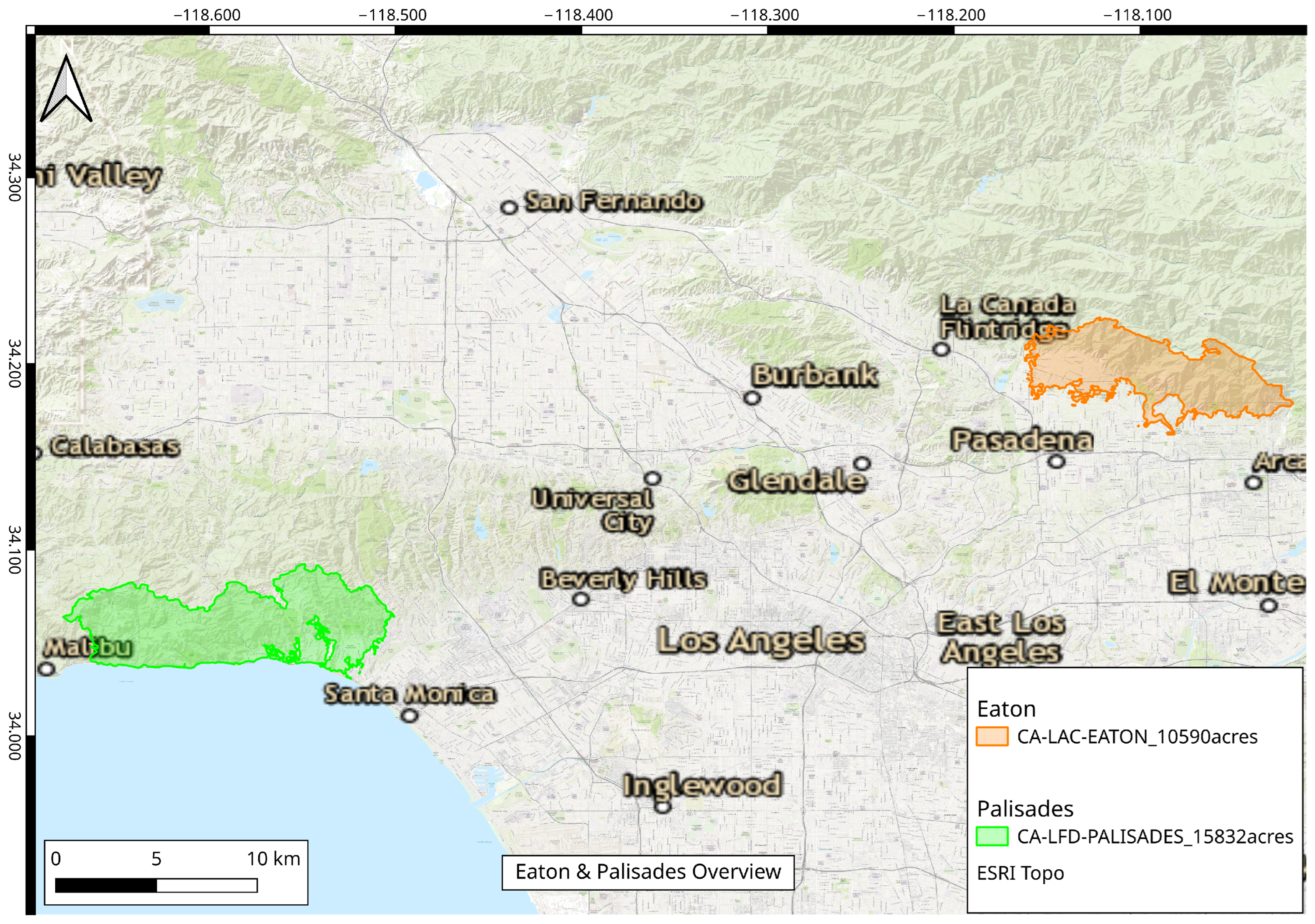
At 10:30 am on 7 January 2025, the Palisades Fire started in Los Angeles and quickly became a wildfire as Santa Ana winds pushed flames rapidly down canyons to the coast. Conditions became increasingly hazardous, with wind gusts reaching 80 mph that day. The California Office of Emergency Services (Cal OES) Fire Integrated and Real-time Intelligence System (FIRIS) [1] aircraft collected its first perimeter of the fire at 1:21 pm, measuring 770 acres of burned area in these first three hours of the fire. With mountainous terrain, access in and out of the Pacific Palisades and Malibu was difficult for residents and firefighters. As the Palisades Fire continued to rage, the Eaton Fire began in the San Gabriel Mountains north of Altadena around 6:00 pm that same day. As winds continued, many additional fires began in subsequent days, including the Hughes, Hurst, Lidia, Hawk, Archer, and Sunset Fires throughout Los Angeles County, stretching firefighting resources thin, leaving these fires to burn uncontrolled. The Eaton and Palisades Fires ultimately became the second and third most destructive fires in California history, respectively, only preceded by the Camp Fire in 2018. The Palisades Fire burned 23,707 acres, destroyed 9413 structures, and killed 19 people. The Eaton Fire burned 14,021 acres, destroyed 6833 structures, and killed 12 people [2]. Figure 1 shows the extents of the Palisades and Eaton fires on 8 January 2025, as used in our analysis.

In the first several hours of an emerging wildfire, fire departments will perform a damage assessment to determine the extent of urban destruction and regions at risk to inform emergency declarations, resource allocation, and recovery efforts. A method to generate confident estimates of damaged infrastructure in a timely manner is essential to expedite this process for requesting appropriate resources.

In this paper, we describe a machine learning approach that leverages multiple data sources and innovative data processing techniques to categorize damaged structures due to wildfire from imagery. Unlike most existing machine learning-based techniques for wildfire damage assessment, which rely on visible RGB bands, our novel approach uses heat signatures from aerial thermal imagery. Thermal data addresses visibility issues common in wildfire scenarios, such as smoke, cloud cover, and variable lighting conditions that are challenging with visible data, as seen in Figure 2. With the deployment of on-demand aerial imagery from the Cal OES FIRIS program, we identify the opportunity to perform damage assessment earlier than high-resolution satellite data can deliver and more efficiently using thermal images and machine learning.

The main contributions of this work are as follows: (1) pipeline for processing aerial image sequences to generate a georectified mosaic representing the region of interest; (2) process for integrating multiple data sources (aerial thermal imagery, building footprints, fire perimeters, and expert-provided damage labels) to extract features for model training; (3) comprehensive analysis of different data products along various dimensions (imagery resolution, thermal bands, and data types) to determine the optimal data product for delivering fast and accurate assessment; (4) machine learning model with cross-region evaluation and domain adaptation for robust classification of structural damages; and (5) detailed evaluation of the approach on the 2025 California wildfires, Eaton and Palisades. The resulting system offers an effective approach for rapid and reliable evaluation of burned structures, suitable for operational wildfire damage assessment.

1.2. Related Work

In recent years, artificial intelligence (AI) techniques have been used in various ways to automate wildfire damage assessment from imagery. Predominantly, the existing work evaluates satellite imagery after the fire has ended. An example of this is the work of Galanis et al. [3], which creates a damage assessment classifier of damaged versus not damaged structures post-fire by providing segmentation and subsequent classification tasks in their model. The model is trained and validated using the xBD library [4], which contains RGB 0.8 m satellite imagery of five wildfires. The xBD library was also used to train the deep learning model in [5] using satellite imagery before and after the incident. Farasin [6] uses imagery from the moderate-resolution Sentinel-2 satellite after the fire is extinct to detect broad regions of burn severity, which cannot distinguish individual buildings at that resolution. The meta-analysis in Shafian [7] reviews 370 papers applying machine learning and remote sensing to building damage assessment of many disaster types. Their review, particularly of papers pertaining to aerial or satellite image analysis, shows that these papers all rely on RGB imagery. Thermal data is referenced to detect thermal anomalies (e.g., campfires and other human activity), not to assess building damage.

Luo et al. [8] use a vision transformer (ViT) to classify building damage from ground-level optical (RGB) imagery. Though these images can provide detailed views of buildings, they are collected by field inspectors after a wildfire and thus are not immediately available after a fire event. Additionally, the availability and quality of building photos vary widely.

Our novel approach uses thermal imagery, collected from aircraft on demand during the fire, for machine learning damage assessment. This overcomes problems with optical images when smoke is present or when there are sub-optimal lighting conditions and time to delivery from satellite data or field-collected ground survey images. The FIRIS aircraft data are available shortly after flights have taken place, enabling analysis on the same day of collection, providing faster-than-ever damage assessment.

ESRI provides a deep learning model for post-disaster damage assessment trained on airbus satellite imagery using RGB 8-bit imagery [9]. Similarly to our approach, building footprints are used for feature extraction, though the exact method is not discussed. Satellite and aerial optical imagery are used as input. Our approach uses thermal data instead, which offers the benefit of enhanced visibility through smoke, haze, and cloud cover. Additionally, our approach can classify structural damage into multiple categories instead of just damaged/undamaged, providing finer analysis details.

Du & Feng [10] propose a method for analyzing post-wildfire building damage using interferometric synthetic aperture radar (InSAR) techniques. This method considers vertical surface deformations caused by intense heat and subsequent cooling to infer building damage rather than directly observing structural damage. Though SAR offers imaging capability under different weather and lighting conditions, this approach requires pre- and post-fire satellite SAR imagery for comparison. Obtaining corresponding and appropriately temporally spaced pre- and post-fire radar imagery may be difficult. Additionally, the authors noted that the medium-resolution SAR data used is not sufficient to capture individual building damage.

A previous version of our approach was introduced in [11]. In this paper, we extend that work in several ways. Several imagery data products are evaluated to determine the efficacy of each with respect to both processing speed and classification performance. Different thermal bands (SWIR, MWIR, LWIR, and thermal composites), mosaics of different resolutions, and different data types (8-bit vs. 16-bit) are analyzed. The model setup is modified to incorporate fire perimeters for more robust training, cross-fire inference for more realistic evaluation, and histogram matching for domain adaptation during inference. Finally, the approach is applied to more recent wildfires, namely the 2025 Eaton and Palisades Fires in California.

2. Materials and Methods

2.1. Data

The Palisades and Eaton Fires started on the same day, under the same weather conditions, and in the same region (Figure 3), which provided an opportunity to collect data on both from the same aerial sensor. We train the machine learning (ML) model on one fire and test it on the other to explore the transferability of this model.

Our approach utilizes imagery from the Fire Integrated and Real-time Intelligence System (FIRIS) as a data source. FIRIS was established in 2019 as a Southern California pilot program and became a formal state-wide permanent program within Cal OES in 2020. This program was developed to provide on-demand support to municipal fire departments responding to wildfires. Real-time data collected by aircraft is used in simulations to show potential fire growth. That data then flows to the hands of firefighters on the ground via mobile devices for better-informed response efforts. The two FIRIS aircraft collect multispectral imagery and perimeters of fire via an Overwatch TK sensor and an FLIR camera, mounted to the bottom of the King Air multi-engine fixed-wing aircraft. During the collection of the fire perimeter, the TK sensor collects imagery with four infrared bands in addition to the visible bands.

Specifically, the data used for this project come from the Overwatch TK-9 Sensor [12] The flight image sequences were collected on the following dates and times: Palisades 8 January 2025 11:49 PST and Eaton 8 January 2025 18:26 PST It has visible RGB, near- (NIR), short-wave (SWIR), mid-wave (MWIR), and long-wave (LWIR) infrared bands. For the Palisades and Eaton Fires, we evaluated the SWIR, MWIR, and LWIR band imagery, both individually and combined into a standard thermal composite Quick Mosaic sensor product (false-color RGB with Red: MWIR; Green: LWIR; and Blue: SWIR).

The imagery in this study was collected at approximate altitudes between 4750 and 4770 m and a camera horizontal field of view of 14.588 degrees in the LWIR, resulting in a pixel size of approximately 1 square meter (spatial resolution), with some slight variation throughout the image tiles due to the aircraft’s varying height above ground throughout the collections. The Quick Mosaics are generated with the DEFLATE compression method, which does not appear to affect spatial resolution, thus providing a product of smaller file size but not a downsampled spatial resolution. This process is performed within the proprietary Overwatch TK9 software platform. The thermal composite products normalize the subtle resolution differences between SWIR, MWIR, and LWIR to 1 square meter.

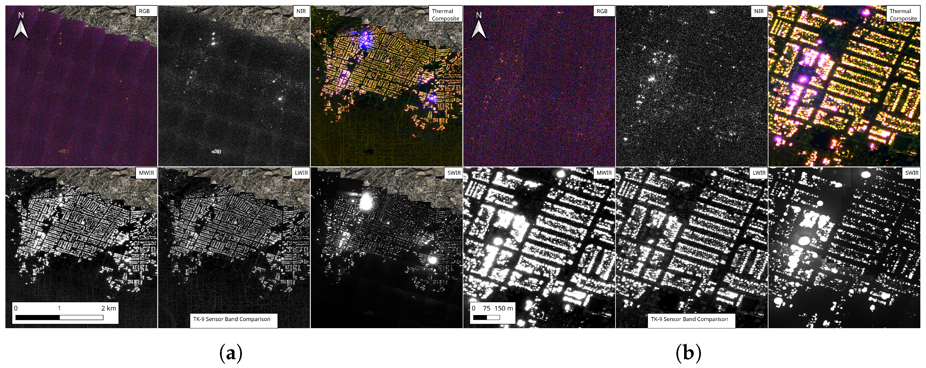
In previous aerial thermal imagery damage assessments, we found that the optimal thermal band is often context-dependent and unique to each fire, with factors such as fire intensity and ambient temperature affecting feature visibility. In the case of both the Palisades and Eaton Fires, the band with the highest level of detail without overexposure was the LWIR. This observation is also supported by the quantitative results in Section 3, where the machine learning experiments indicate that the LWIR band provides the strongest overall performance on our data. SWIR was unable to penetrate areas with thick smoke, and the MWIR band tended to be overexposed in the densest urban areas of the two fires. See Figure 2 and Figure 4 comparing the TK-9 bands for Palisades and Eaton, respectively.

The Microsoft Building Footprints [13] were used as the ground truth for the location and size of existing structures within the burn scar. They were used to query the thermal imagery heat intensities, using their precise locations as the basis for evaluating the imagery. Microsoft generated this dataset by semantic segmentation and polygonization of aerial image pixels from 2014–2021 Bing Maps imagery, incorporating Maxar and Airbus imagery, and made it publicly available.

The California Department of Forestry and Fire Protection (CAL FIRE) [14] deploys a damage inspection (DINS) team after a large wildfire has ended in California to inspect every structure within the burned perimeter and determine whether it is damaged, destroyed, or unaffected [15] This DINS data is then made available after a period of weeks to the public. It is a detailed and accurate ground truth dataset that is used to train our machine learning model.

Active fire perimeters are also used in this study. They are created by a human sensor operator in the FIRIS aircraft leveraging thermal imagery to trace the extent of the fire. They are traced within 5–20 min of the imagery collection from the TK9. The perimeter is used to clip the extent of the analysis so as not to include DINS labels and buildings that are not yet within the burn scar, as described in Section 2.3.2.

2.2. Imagery Processing

An additional novel approach in this paper is to take advantage of the “Quick Mosaic” raster products that the Overwatch TK sensor software produces. The Quick Mosaic product is raster imagery with a reduced file size of the entire image collection that allows for faster processing so that it can be delivered in real time during flight. The software stitches, blends, and georeferences all image tiles from a continuous flight into a single orthomosaic image. Earlier work [11] leveraged only the full-resolution original tile imagery, but the benefit of using the Quick Mosaic means that analysts can obtain the imagery delivered while the plane is still in the air. The TK software collects high-resolution image tiles. After collection, the software generates Quick Mosaics at 8-bit and 16-bit resolution. The full-resolution image tiles must be georeferenced with a third-party software, such as Agisoft Metashape in our case. Experiments using the LWIR band of these three products were conducted, as detailed in Section 3.2.1.

These three image product types are shown in Figure 5 and described in

Table 1. Imagery formats for Palisades and Eaton Fires.

Image Type	Data Type	File Format	Geocorrection Level	CRS
Quick Mosaic	8-bit	GeoTIFF	Fastest	EPSG 4326
Quick Mosaic	16-bit	GeoTIFF	Best	EPSG 4326
FullRes	16-bit	GeoTIFF	Manual	EPSG 4326

.

Additional georectification of the Quick Mosaics in QGIS (versions 3.34 Prizren, 3.40 Bratislava, and 3.44 Solothurn) [16] was necessary in order to ensure proper alignment with the building footprint datasets. Without additional refinement of the mosaic alignments, the heat intensities of burning buildings in the thermal images would not coincide with the same building’s footprint, as shown in Figure 6, which is required for the training and testing of our ML algorithm. This refinement was accomplished by using the QGIS Georeferencer [17] tool and adding ground control points (GCPs) manually in an iterative fashion until building footprint–IR image alignment was sufficient throughout each flight’s and band’s Quick Mosaic. The reference images used for georeferencing were obtained through the QGIS QuickMapServices plugin (version 0.21.4) [18] and are as follows: ESRI Satellite, Bing Satellite and Bing Aerial basemaps. The Georeferencer settings used are shown in

Table 2. QGIS Georeferencer settings for Palisades Flight.

Image Type	Transform Method	Resampling Method	Compression
Quick Mosaic 8-bit	Thin Plate Spline	Cubic B-Spline (4 × 4 Kernel)	Deflate
Quick Mosaic 16-bit	Thin Plate Spline	Cubic B-Spline (4 × 4 Kernel)	Deflate
Full-Res 16-bit	Thin Plate Spline	Cubic B-Spline (4 × 4 Kernel)	N/A

. We have found that the misalignment of this imagery is on average 12 m, with varying error depending on the obliqueness of the imagery when collected.

For image collections that required more than one Quick Mosaic to collect the full extent of the fire, Quick Mosaics for each flight path were merged into a single mosaic using the QGIS Raster Merge [19] tool to form a combined image encompassing the full fire extent at the time of each flight. This tool simply aligns adjacent images using their overlapping regions. These merged images were then more precisely georectified using the Georeferencer, as previously described.

Metashape (Agisoft Metashape version 2.1.0) [20] was used to create an orthomosaic of the original individual full-resolution PNG images. The images received from the aircraft were imported into Metashape and then aligned using the corresponding reference file. Once the initial orthomosaic was generated, GCPs were used to correct any misalignment or distortion. This was performed by adding markers to significant features in the imagery and then repeating the placement of the same marker in each individual image that contained that location. GCPs were distributed throughout each mosaic and added as needed to ensure the images were aligned correctly with the reference base map. Image alignment was then repeated and a final orthomosaic was generated.

However, after reviewing the final othromosaic products generated by Metashape, it was discovered that additional refinement of their geolocation was also necessary (Figure 6, 16-bit FR LWIR Unmodified vs. Modified), following the same method as was used for refining the Quick Mosaics.

2.3. Data Preparation

2.3.1. Feature Extraction

Building footprint data from Microsoft was used to identify the locations of structures within the fire extents of the Palisades and Eaton Fires. To establish ground truth labels for these structures, we used the CAL FIRE DINS dataset, which provides geolocated points representing the inspected structures, each annotated with a categorical label indicating the level of damage caused by the wildfire: Destroyed, Major Damage, Minor Damage, Affected, and No Damage. To associate these DINS labels with the corresponding buildings in the Microsoft buildings footprint dataset, we perform a point-in-polygon spatial join, where each DINS point is matched to a building footprint if it lies within the footprint’s polygon geometry. The damage label from the DINS point is then assigned to the corresponding building.

However, in some cases, DINS points may be slightly misaligned relative to the building footprints due to geolocation inaccuracies, leading to unmatched points. To address this, we expand the footprint polygons outward by adding a buffer zone around each building footprint. The matching process is applied with buffer sizes of 5 m and then 10 m, allowing nearby points to be captured if they fall just outside the original footprint boundaries. Despite these adjustments, some DINS points and building footprints may still remain unmatched. These points are excluded from further analysis, as the unmatched DINS points may correspond to structures that are not represented in the Microsoft dataset. In cases where a DINS point falls within multiple buffered building footprints, the DINS point is assigned to the closest building footprint based on the Euclidean distance.

Following the association between building footprints and DINS points, we extract thermal information from the infrared mosaic images for each matched pair. The footprint polygon is used to clip the corresponding region from the mosaics, and heat intensity statistics, specifically, the minimum, mean, and maximum pixel intensity values are computed from within the clipped area. For thermal composite mosaics containing three spectral bands (MWIR, LWIR, and SWIR), we compute the same statistics for each band, resulting in nine features per building–ground truth pair. These extracted thermal features form the input dataset for the machine learning model, which is trained to classify buildings affected by an unseen wildfire into one of the DINS damage categories to enable automated, data-driven post-wildfire damage assessment.

2.3.2. Fire Perimeter Restriction

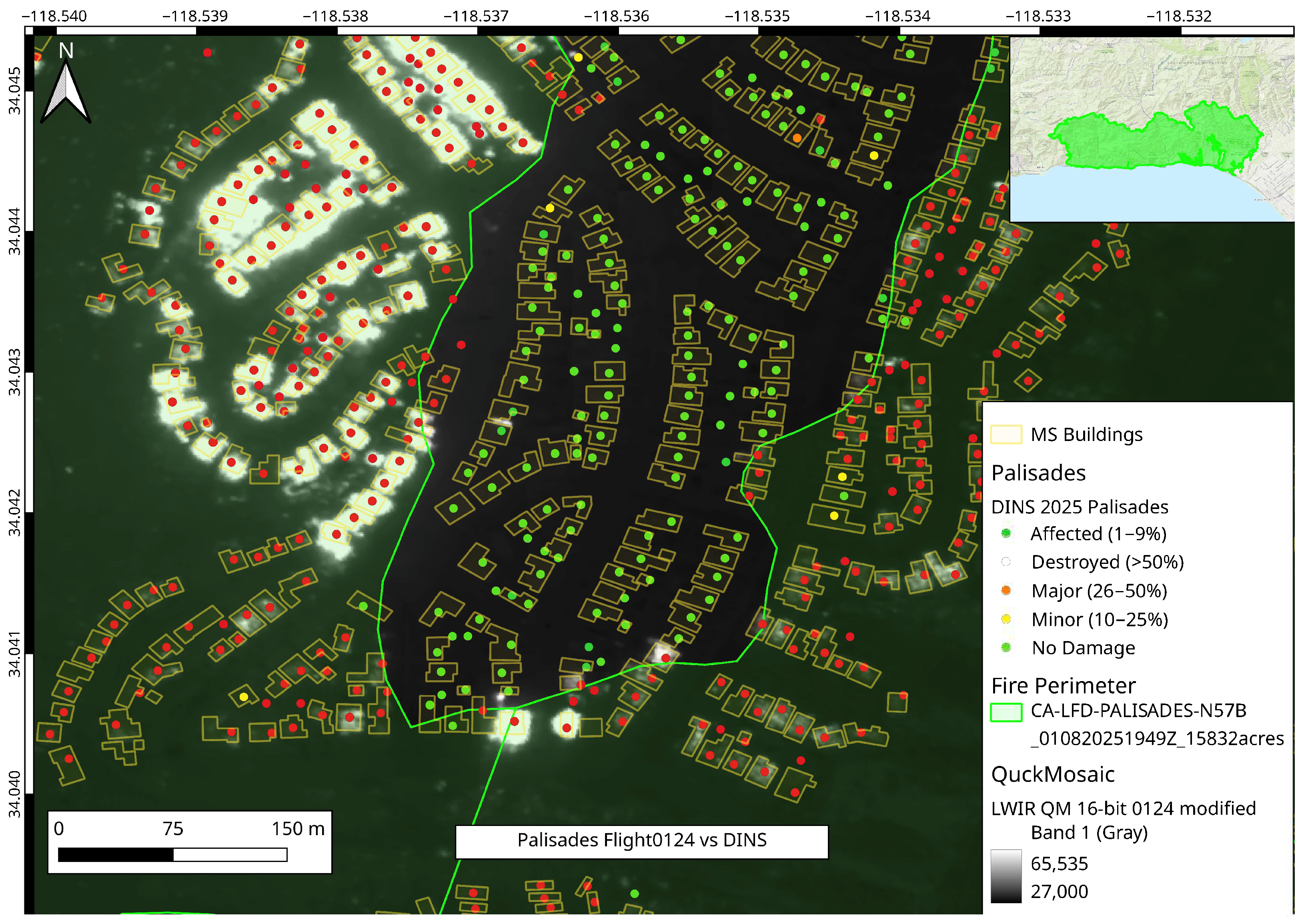
The ground truth points and labels derived from the CAL FIRE DINS data lack temporal information; we do not know when in the life of the fire each structure was ignited. In order to use only the relevant structures of interest, we clip the DINS data and paired building footprints with the FIRIS perimeter generated at the time of the image collection. These perimeters delineate the actively affected area during the time of the flight. This excludes structures that fall outside the perimeter, thereby preventing the model from being trained on confounding or temporally inconsistent data. This is illustrated in Figure 7.

Consequently, there may be instances within the fire perimeter where some buildings had not yet burned at the time the image was captured but were damaged by the fire hours or even days later. Because these structures are eventually affected, the DINS dataset may label them as Destroyed (or another damage category). However, since the IR imagery was taken before the damage occurred, the corresponding pixel values around these buildings may show low or no heat intensity, leading to misleading features for model training. The imagery used for this study was taken after day 1 of the Eaton, and after day 3 of the Palisades, which is where the greatest urban conflagrations occurred, providing many thousands of structures from each fire to train and test the model with statistical significance. But, due to this timing, in both cases, some structures may have also burned and cooled at the time of collection.

2.3.3. Domain Adaptation Using Histogram Matching

Histogram matching is a normalization technique used to adjust the histogram (or distribution) of a source dataset so that it matches that of a reference dataset [21]. The process involves computing the cumulative distribution functions (CDFs) of both the source and reference data and then remapping each value in the source data to the corresponding value in the reference distribution [22]. Figure 8 from [23] illustrates the CDF-based histogram matching process. The cumulative histogram is first computed for each dataset. Then, for a given input value $x_i$, its cumulative histogram value $G\left(x_i\right)$ is used to find the corresponding cumulative distribution value in the reference dataset, $H\left(x_j\right)$, and $x_i$ is then replaced by $x_j$. This approach is commonly used in image preprocessing to improve domain adaptation and reduce variability introduced by differences in sensors, lighting, or acquisition conditions [24,25,26].

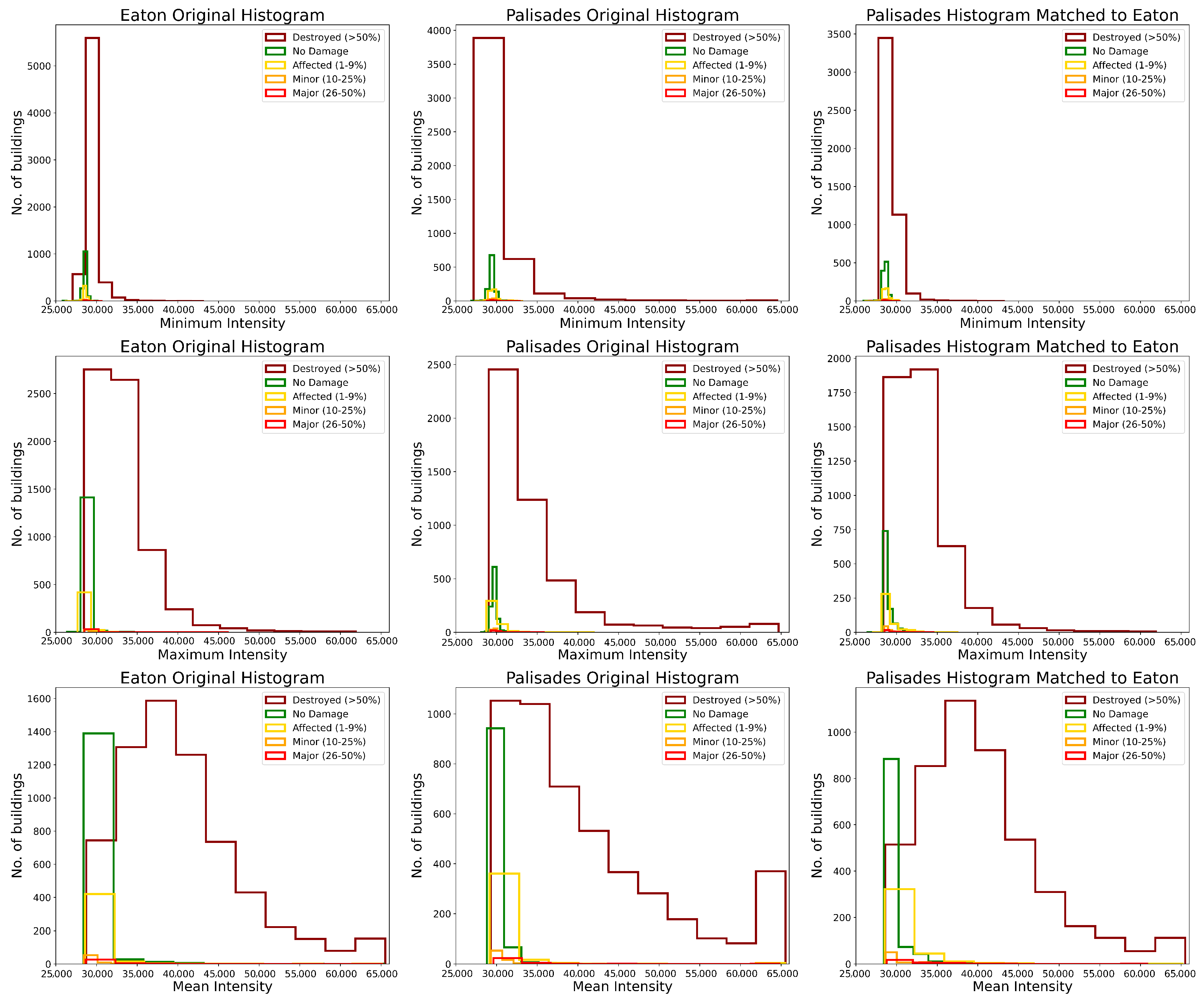
In our methodology, we perform domain adaptation by applying histogram matching to the features extracted from the mosaic images, specifically the minimum, maximum, and mean intensity values of the test dataset, using the corresponding feature histograms from the training dataset as a reference. The operation was implemented using the ‘match_histograms’ method from the skimage.exposure subpackage of the scikit-image library [27]. This normalization helps mitigate differences caused by the time of day during which the infrared images for the Palisades and Eaton Fires were captured, as well as variations in overall intensity signatures arising from topographical differences between the two regions.

Figure 9 illustrates the effect of this normalization, showing the histograms of the Palisades features before and after applying histogram matching, with the corresponding Eaton feature histograms as the reference distribution.

2.4. Machine Learning Setup

After the feature extraction and preprocessing steps, which prepare the data and intensity readings from the IR mosaics of the Palisades and Eaton Fires for machine learning (ML) applications, we proceed to train an ML-based classification model. For this study, we employ a Random Forest classifier, with its hyperparameters optimized through a 5-fold cross-validated grid search on the training data. In addition to conventional ML setups where a single dataset is partitioned into training and testing subsets (e.g., an 80–20 split), our approach intentionally separates the data by fire for most of the experiment setups. Specifically, we train the model using all data from one fire and evaluate its performance on the entirety of the other fire’s data. This cross-fire evaluation strategy simulates a realistic operational scenario where a model trained on historical fires is applied to assess building damage in a new, unseen fire event. Such an approach tests the model’s generalization ability and its potential for real-world deployment in rapid post-fire damage assessment pipelines. All ML experiments in this study are conducted under both multi-class and binary classification settings. The ground truth labels derived from the CAL FIRE DINS dataset categorize structures into six classes based on damage levels:

• Destroyed —More than 50% damage;
• Major—Between 26 and 50% damage;
• Minor—Between 10 and 25% damage;
• Affected—Less than 10% damage;
• No Damage;
• Inaccessible.

Structures labeled as Inaccessible are excluded from the analysis due to the absence of verifiable damage information. For the multi-class classification problem, the remaining five categories (Destroyed, Major, Minor, Affected, and No Damage) are considered as distinct output classes. For the binary classification setting, based on the distribution of samples across classes (as summarized in

Table 3. Damage class dstribution for Palisades and Eaton Fires.

Fire	No Damage	Affected	Minor	Major	Destroyed
Palisades	1029	393	80	33	4217
Eaton	1446	452	73	35	6671

), Affected and No Damage are grouped into a category representing ‘Low or No Damage’, while Minor, Major, and Destroyed are combined into another category representing ‘Significant Damage’. To mitigate the major class imbalance problem present in both the multi-class and binary settings, the Random Forest classifier is configured with the class_weight parameter set to balanced. The binary class formulation further helps address imbalance and provides a more actionable Damage–No Damage distinction relevant for emergency response and recovery operations.

3. Experimental Setup and Results

3.1. Experimental Setup

We perform multiple experiments across different configurations of the mosaic data to systematically evaluate cross-fire classification performance between the Palisades and Eaton Fires. These experiments are designed to identify the standard form of IR mosaic data for training and inference in ML-based damage assessment tasks. All the experiments were conducted on a system with dual Intel Xeon E5-2670 (Santa Clara, CA, USA) processors (8 cores each, 2.60 GHz; 16 cores total) and 64 GB of RAM. The experiments span three key criteria: resolution, infrared (IR) band, and data type.

• Resolution: Full Resolution vs. Quick Mosaic
  The first set of experiments compares model performance between full-resolution (FR) and Quick Mosaic (QM) IR data. Full-resolution mosaics are refined post-flight products that undergo extensive human-assisted rectification and alignment, providing high spatial precision but requiring considerable processing time before they can be used. Quick Mosaics, on the other hand, are automatically stitched and rapidly released following data collection, enabling near-real-time readiness with minimal preprocessing. This experiment evaluates the effectiveness of these two data products in supporting ML-based damage classification, with a focus on understanding how differences in data preparation and spatial detail influence overall model performance.
• IR Bands: LWIR vs. MWIR vs. SWIR vs. Thermal Composite (TC)
  The second set of experiments evaluates model performance across different infrared spectral bands, namely long-wave infrared (LWIR), mid-wave infrared (MWIR), short-wave infrared (SWIR), and thermal composite (TC) imagery. Each single-band mosaic captures a distinct portion of the thermal spectrum, providing complementary information on fire intensity and post-fire heat distribution. The thermal composite (TC) Quick Mosaics integrate three bands—LWIR, MWIR, and SWIR—into a single three-channel composite product. Since each spectral band is originally provided separately, using TC mosaics could potentially eliminate the need for individual preprocessing pipelines and per-band model evaluations. These experiments therefore investigate whether TC imagery can serve as a standard unified data product capable of preserving the discriminative power of separate bands. This comparison is crucial, as the relative performance of MWIR and LWIR in particular may vary based on environmental conditions such as time of day, fire intensity, topography, and atmospheric effects.
• Data Type: 16-bit vs. 8-bit
  These experiments are designed to evaluate the impact of radiometric resolution on classification performance. The initial default is the 8-bit Quick Mosaic, which is efficient for storage, faster to process, and easier for humans to inspect when analyzing thermal signatures in damaged buildings. The 16-bit Quick Mosaics preserve the full range of sensor intensity values, capturing subtle variations in thermal response that may be important for accurately distinguishing damage levels [28]. In contrast, the 8-bit products, while easier to store and interpret, may lose some of these fine details that a machine learning model could use. This experiment evaluates whether the extra computational and storage cost of 16-bit mosaics is justified by improvements in model performance.

3.2. Results

This section summarizes the results of the damage assessment experiments conducted for the Palisades and Eaton wildfires using a Random Forest classifier. Results are presented for both multi-class and binary classification tasks. The classification metrics used to evaluate each experiment are accuracy, F1-score, and ROC-AUC score.

The possible outcomes of a classification made by an ML model can be one of the following: true positive (TP)—a correct positive prediction; false positive (FP)—an incorrect positive prediction; true negative (TN)—a correct negative prediction; and false negative (FN)—an incorrect negative prediction. Based on these outcomes, the accuracy of a model on a test set is the ratio of all predictions that the model correctly made over the total predictions, as shown in Equation (1).

$$\mathrm{Accuracy}={\displaystyle \frac{TP+TN}{TP+TN+FP+FN}}$$

(1)

When the dataset is class-imbalanced, relying solely on accuracy can be insufficient. In such cases, the F1-score provides a more balanced evaluation. It is particularly useful when minimizing both false positives and false negatives is important and is formulated as shown in Equation (2).

$$\mathrm{F}1-\mathrm{score}={\displaystyle \frac{TP}{TP+\frac{1}{2}(FP+FN)}}$$

(2)

The Area Under the Curve for the Receiver Operating Characteristic (ROC-AUC) [29] quantifies the model’s ability to distinguish between classes across varying classification thresholds, generally ranging from 0 to 1. The ROC curve itself plots the True Positive Rate (TPR) (3) against the False Positive Rate (FPR) (4) over each threshold. A higher ROC-AUC value indicates a stronger ability of the model to correctly differentiate between positive and negative classes across different thresholds.

$$\mathrm{TPR}={\displaystyle \frac{TP}{TP+FN}}$$

(3)

$$\mathrm{FPR}={\displaystyle \frac{FP}{FP+TN}}$$

(4)

All experiments were repeated three times using different random seeds, and the mean values for each evaluation metric are reported, with the standard deviations shown in parentheses. The best results for each experiment are highlighted in bold for every evaluation metric. In cases where two results are very close based on their standard deviations, both values are highlighted. The subsequent subsections focus on specific data comparisons, which include the following: (i) spatial resolution (full resolution vs. Quick Mosaic), (ii) infrared band combinations (SWIR, MWIR, LWIR, and thermal composites), and (iii) data type (16-bit vs. 8-bit).

3.2.1. Full Resolution vs. Quick Mosaic

Table 4. Full resolution vs. Quick Mosaic—LWIR band, 16-bit, Palisades data. Best results are in bold text.

		Multi-Class			Binary
Fire	Res	ACC	F1	AUC	ACC	F1	AUC
Palisades	QM	0.8633 (0.0064)	0.8516 (0.0007)	0.9544 (0.0014)	0.9178 (0.0030)	0.9184 (0.0034)	0.9573 (0.0026)
	FR	0.8461 (0.0009)	0.8267 (0.0015)	0.9351 (0.0007)	0.8867 (0.0013)	0.8893 (0.0011)	0.9448 (0.0014)

presents the results of experiments comparing model performance when trained and tested on full-resolution mosaics versus Quick Mosaics. The experiment was conducted using the Palisades fire dataset, with an 80–20 train–test split applied to both the Quick Mosaics and full-resolution versions. To ensure a fair comparison, we use the 16-bit data type and LWIR band version for both the Quick Mosaic and the full-resolution image. This experiment helps to determine the appropriate resolution type to adopt for future analyses. The results indicate that Quick Mosaics consistently outperform full-resolution mosaics across evaluation metrics, for both multi-class and binary classification tasks. A possible reason for this performance difference is that the full-resolution mosaics contain distortions and alignment issues that may affect feature extraction, as elaborated further in the Discussion Section 4.2.3. These findings provide strong evidence in favor of using Quick Mosaics for future wildfire damage assessment tasks. Quick Mosaics significantly reduce preprocessing and rectification requirements compared to full-resolution mosaics, while still achieving strong performance suitable for further use.

3.2.2. IR Band Comparison

This subsection focuses on comparing model performance across different infrared (IR) bands, using Quick Mosaics for all experiments. All bands use 16-bit Quick Mosaic data to ensure a fair comparison. The results in

Table 5. IR band comparison—Quick Mosaics, 16-bit, Palisades and Eaton data. Best results are in bold text.

			Multi-Class			Binary
Train	Test	Band	ACC	F1	AUC	ACC	F1	AUC
Palisades	Eaton	SWIR	0.6887 (0.0028)	0.6534 (0.0021)	0.6065 (0.0079)	0.6609 (0.0019)	0.6731 (0.0021)	0.6294 (0.0039)
		MWIR	0.8548 (0.0015)	0.8548 (0.0011)	0.9557 (0.0003)	0.9168 (0.0010)	0.9181 (0.0010)	0.9648 (0.0017)
		LWIR	0.8867 (0.0011)	0.8694 (0.0009)	0.9609 (0.0010)	0.9394 (0.0010)	0.9394 (0.0009)	0.9734 (0.0003)
		TC	0.8729 (0.0047)	0.8613 (0.0032)	0.9608 (0.0029)	0.9206 (0.0013)	0.9204 (0.0015)	0.9675 (0.0006)
Eaton	Palisades	SWIR	0.6451 (0.0009)	0.6424 (0.0007)	0.6054 (0.0031)	0.6879 (0.0019)	0.6911 (0.0014)	0.6018 (0.0028)
		MWIR	0.8004 (0.0071)	0.7832 (0.0039)	0.9051 (0.0024)	0.8807 (0.0010)	0.8810 (0.0010)	0.9312 (0.0047)
		LWIR	0.8393 (0.0023)	0.8300 (0.0016)	0.9278 (0.0033)	0.9048 (0.0012)	0.9051 (0.0010)	0.9405 (0.0022)
		TC	0.8380 (0.0019)	0.8321 (0.0017)	0.9280 (0.0040)	0.9050 (0.0011)	0.9053 (0.0009)	0.9259 (0.0064)

show that the LWIR band consistently outperforms the MWIR and SWIR bands across all evaluation metrics and for both classification tasks, indicating that LWIR carries the most informative intensity signatures for the fires examined in this study. The thermal composite (TC), which integrates information from all three bands, performs better than MWIR and SWIR individually and achieves results comparable to LWIR alone in many cases. In the table, where the difference between LWIR and TC results is not statistically significant, both are bolded.

3.2.3. 16-Bit vs. 8-Bit

This subsection presents the results of the data type comparison experiments. We used 8-bit and 16-bit Quick Mosaics of the LWIR band to evaluate how sensor resolution affects both model performance and computational efficiency. In addition to the evaluation metrics used in previous experiments (accuracy, F1-score, and ROC-AUC score), we also compared the computational runtime (in seconds) for the 8-bit and 16-bit datasets. All experiments were executed on the same machine described earlier, utilizing all 16 CPU cores.

As shown in

Table 6. 16-bit vs. 8-bit—Quick Mosaics, LWIR band, Palisades and Eaton data. Best results are in bold text.

			Multi-Class			Binary
Train	Test	Data Type	ACC	F1	AUC	ACC	F1	AUC	Time (in s)
Palisades	Eaton	16-bit	0.8867 (0.0011)	0.8694 (0.0009)	0.9609 (0.0010)	0.9394 (0.0010)	0.9394 (0.0009)	0.9734 (0.0003)	38.39 (0.78)
		8-bit	0.8794 (0.0015)	0.8710 (0.0011)	0.9629 (0.0009)	0.9348 (0.0008)	0.9362 (0.0008)	0.9773 (0.0002)	29.76 (1.20)
Eaton	Palisades	16-bit	0.8393 (0.0023)	0.8300 (0.0016)	0.9278 (0.0033)	0.9048 (0.0012)	0.9051 (0.0010)	0.9405 (0.0022)	48.41 (0.70)
		8-bit	0.8035 (0.0045)	0.7962 (0.0021)	0.8721 (0.0008)	0.8625 (0.0021)	0.8632 (0.0016)	0.8788 (0.0022)	31.56 (0.94)

, training and testing with 8-bit data is noticeably faster than with 16-bit data. However, in terms of classification performance, the results vary depending on the training–testing configuration. When the model is trained on the Palisades dataset and tested on the Eaton dataset, the performance is comparable between the two data types, with 16-bit data showing only a slight advantage. In contrast, when the model is trained on Eaton and tested on Palisades, the 16-bit data consistently outperforms the 8-bit data across all classification metrics by a significant margin. While the 8-bit experiments are faster, the runtime difference is not substantial enough to justify sacrificing model accuracy. For a critical task such as wildfire damage assessment, accuracy and reliability are far more important than marginal gains in computational speed.

4. Discussion

4.1. Significance of Our Results

The concurrent and proximal Palisades and Eaton Fires, under broadly the same atmospheric conditions of the wind event, provided a unique circumstance to investigate the potential similarities and differences between the two with respect to our damage assessment models. Our results show a marked difference between the two cross-region performance metrics even after histogram matching, with the Palisades-trained model performing best. We speculate that this may be because there were more varied intensities of burning structures in the Palisades imagery as compared to the more uniform Eaton intensities (Figure 10), resulting in a more generalizable model. The Palisades Fire experienced more varied urban fire growth over 3 days, as compared to Eaton, which reached a similar number of structures damaged over its second night of growth. However, it remains unclear what other confounding factors may also be contributing to this difference in performance, which likely include the following:

• Differences in topography, which influences wind speed and direction, since Palisades is predominantly hilly and separated by canyons versus the mostly contiguous, flat, and gently sloped Eaton area downwind of the San Gabriel Mountains; for the effect of topography on the image preprocessing, we found that the areas of high topographic relief affected the amount of distortion in the generated full-resolution and QuickMosaic mosaics.
• Differences in predominant fuels based on vegetation types at the Wildland–Urban Interface (WUI), since Palisades is at the coast and likely experiences more regular moisture and subsequent vegetation growth, while Eaton is approximately 25 miles (40 km) further inland and presumably much drier (Figure 3).
• Differences in the fire environment impacting the probability of ignition (PIG) and neighborhood burn times, potentially due to building density, landscaping, construction type (residential, commercial, etc.) and material (wood-frame, concrete, etc.), age (building codes), and form (density and setbacks).
• And/or differences in the time of day the imagery was collected and its global effect on intensity values, particularly where the low-intensity damage thresholds separating burning structures and objects at elevated fire-warmed and ambient temperatures increasingly overlap.

Examining the differences between these two coinciding fires remains an area with numerous avenues for further investigation.

The results of this work show there is a benefit to the Quick Mosaic image format that the Overwatch software delivers. The format enables this rapid analysis without a reduction in the spectral data when using 16-bit. The reduced file size decreases the transmission time, which can be performed while the plane is still in the air, and also reduces image preprocessing and analysis time. As seen in these Santa Ana wind-driven urban fires, there is a proven benefit to the thermal image bands for damage assessment in the early stages of a fire. The MWIR and LWIR can penetrate thick smoke and clouds and can still provide good feature contrast, assuming optimal ambient temperatures.

4.2. Data Challenges

4.2.1. Building Footprint Data

This research used the Microsoft Building Footprints as the knowledge base for identifying structure locations. However there are other openly available building footprint datasets available, including the FEMA Structures [30] and OpenStreetMap [31] datasets. Qualitatively, the Microsoft Buildings dataset was used because it appeared to be more comprehensive in the Palisades and Eaton areas than the other sources. However, in general it has been less accurate in terms of building shape and detecting the presence of smaller and/or obscured structures than other footprint datasets we have examined in past work, such as mobile homes or auxiliary structures. The quality of each dataset appeared variable by region in our earlier experiments. In Los Angeles, the OpenStreetMap data maybe have better coverage and more accurate building shapes but suffer from areas of missing data. Its aspects of greater accuracy may be due to its crowd-sourced review. It is possible that using a different footprint dataset would yield different results. We are considering addressing this issue in future work by (1) generating an optimal product by combining all three sources manually or via a geospatial union of the data and/or (2) using LiDAR to extract building extents from point cloud classifications to supplement missing data.

4.2.2. Damage Inspection (DINS) Data Limitations

DINS data is the only accurate field-recorded information that describes the state of structures after a fire and is therefore the only data we can use to train our model. Because DINS data is generated only after a fire is completely out, there are challenges in using it as ground truth for our analyses, as the imagery we are using is collected one to three days after the fire started. For this reason, we assume that the fire has burned throughout the entire extent within the fire perimeter to train the model. However, we can see that this is not always the case in localized areas of the Palisades and Altadena, which we discuss in Section 4.1. In future work, we intend to manually review each label in the DINS reports with the heat intensity of the associated building at the time of flight and relabel as needed to ensure that the DINS data accurately represents each structure as burning or not burning at the time of image collection.

4.2.3. Imagery

There are several challenges working with the image resolutions and bands chosen for this work. One of the environmental factors affecting the quality of IR imagery for damage assessment is the time of day that a collection has been performed. This mainly concerns how differences between ambient and object temperatures affect the visible details outside of the fire areas. For example, from work with previous fires, we have seen that IR imagery collected in the early evening, when the air temperature and vegetation have begun to cool but roofs and streets are still warm, have a much higher contrast and the distinction between these features is more recognizable. Conversely, IR images collected around midday when the air, roofs, streets, and vegetation are closer in temperature makes it more difficult for a human to confidently identify low-intensity structures. This has an effect on the quality of the georectification since it could impact the accuracy of placing GCPs.

The full-resolution orthomosaics generated with the Metashape software proved difficult to work with. Generating mosaics of these wide regions from the aerial imagery yielded holes, incomplete processing, and significant distortion in varied terrain that led to the misalignment of building footprints with the mosaics. This may be due to the geographic extent of the fire or flight conditions during the data collection process. The selection and placement of ground control points (GCPs) for mosaic georectification, in both Metashape and QGIS, is also subjective and human error is possible. In order to correct these errors, we added GCPs in each mosaic until we felt there was sufficient alignment with the building footprints, with some of the larger mosaics requiring as many as two hundred. This process is time-consuming and requires precision, relying on prominent features matching precisely in both the reference RGB imagery and the thermal imagery.

Since the additional manual georectification of the mosaics is by far the most time-consuming step of this damage assessment methodology, opportunities for further research into automating this process should be pursued and could yield both increased accuracy and reduced processing time, potentially from on the order of hours to minutes. Tools such as Geo-AI or OpenCV may be worth evaluating for this task, though the ability of such algorithms to precisely geolocate IR imagery, whether by matching it to an RGB reference image or by other means, would need to overcome the variable contrast of IR imagery in multiple bands.

When it comes to training ML models, we have shown that the 16-bit imagery has a more comprehensive range of heat intensity, which performs better than the 8-bit data type with an ML model, as we might expect. It has also allowed us to see that the heat range is more variable in Palisades than in Eaton, possibly resulting in different outcomes in generalization when trained on one fire and tested on another.

4.3. Future Work

For future work, we will evaluate the robustness of our approach by testing it on different fires. As discussed above, various factors such as topography and fuels affect the manifestation of fire intensities in imagery, which in turn could affect model classification performance. Evaluating fires with different geographical regions and environments is thus important to understand the generalizability of the approach.

We also plan to integrate deep learning techniques to enhance our approach. Currently, the ML model uses features that are manually designed, like the minimum, maximum, and mean pixel intensities. More advanced texture-based feature extraction techniques like a Gray Level Co-occurrence Matrix (GLCM) [32] and Local Binary Patterns (LBPs) [33] also offer a promising way to further enhance the classification capability of the ML model and will be explored in the future. Deep learning models such as residual network (ResNet) [34] and vision transformer (ViT) [35] automatically learn hierarchical representations directly from raw data, enabling them to model intricate patterns that manually engineered features may miss. By ingesting the image data directly, deep learning techniques can also capture complex spatial–spectral relationships, which are important for tasks with high-dimensional and unstructured inputs such as images. Additionally, the use of transfer learning offers a powerful way to adapt foundation models such as DINOv2 [36] and SAM2 [37] to various specific tasks. We will leverage deep learning in our approach as a next step.

To increase the amount of information provided to the model, we will evaluate the use of RGB and of the thermal composite (TC) further. While IR is effective for detecting damage to structures during active fires, RGB is more effective when structures have cooled. Combining RGB with IR will provide more comprehensive data covering the different stages of fire, leading to more robust damage assessment performance. The thermal composite (TC) Quick Mosaic combines SWIR, MWIR, and LWIR, as discussed in Section 3.2.2. Though our results in this paper indicate that LWIR slightly outperforms TC on most metrics, the composite may be particularly useful in cases where LWIR alone does not provide a strong distinction between damage classes. The availability of multiple bands in TC will also be beneficial for deep learning techniques, which can ingest multi-dimensional inputs and learn which features and feature combinations are important as needed for the classification task. Moreover, TC removes the need to generate and evaluate separate mosaics for individual bands, offering a practical alternative for operational use.

To address data quality issues, we will explore the use of additional sources for building footprints such as LiDAR to provide more complete coverage. Additionally, we will investigate the use of stacking sequences of aerial images and curated DINS data. In order to mitigate the effects of the passage of time between the multiple days of Palisades flights on the evolution of fire intensity and the subsequent variation in the heat of buildings in the IR imagery, we evaluated an image stacking and pixel aggregation method using the GRASS r.series [38] tool in QGIS to generate a single composite mosaic containing only the maximum pixel values from every Palisades flight. We refer to these composite images containing the statistically calculated maximum intensity value from across the input images as StackMAX. The result shows the maximum heat intensity each structure experienced throughout the catalog of images, regardless of timing and flight number. In order to have a true understanding of the status of structures at the time the imagery is taken, the DINS data would need to be modified to reflect the intensities observed. For example, if there is no observable increased intensity where there are structures but the DINS labels show them as having Major damage or being Destroyed, this would indicate that the structures had not begun to burn at the time the imagery was collected and rather sustained damage at some time later. Curating the DINS datasets will likely lead to improved damage assessment performance.

5. Conclusions

We have presented a machine learning approach for automated assessment of structural damage caused by wildfires using thermal aerial imagery. By leveraging multiple data sources in model development—namely satellite-based building footprints, expert-labeled post-fire damage points, fire perimeters, and aerial thermal imagery—the approach can be used to identify various levels of structural damage from just aerial thermal imagery during operational use. Experiments to evaluate different data products established that the 16-bit Quick Mosaic is the optimal data for this application, delivering strong classification performance without the need for time-consuming manual full-resolution mosaic generation. Results on the Eaton and Palisades wildfires demonstrate the effectiveness of this method and its applicability to real-world scenarios.

We have also highlighted several challenges with the data. Our work offers methods for mitigating some of those challenges and underscores outstanding difficulties that are important for the community to recognize.

The findings in this research contribute to advancing the integration of data-driven modeling into damage assessment workflows. Future research will explore strategies to continue to address data issues and to enhance the robustness and generalizability of the proposed approach to further advance the use of AI techniques for effective and efficient operational damage assessment.

References

1. California Governor’s Office of Emergency Services. FIRIS. 2025. Available online: https://www.caloes.ca.gov/office-of-the-director/operations/response-operations/fire-rescue/firis/ (accessed on 1 October 2025).
2. CAL FIRE. Top 20 Most Destructive California Wildfires. 2025. Available online: https://34c031f8-c9fd-4018-8c5a-4159cdff6b0d-cdn-endpoint.azureedge.net/-/media/calfire-website/our-impact/fire-statistics/top-20-destructive-ca-wildfires.pdf?rev=737a1073f76947b4a3bfb960b19f44c7&hash=7CA02D30D9BF46A32D5D98BD108BA26A (accessed on 1 October 2025).
3. Galanis, M.; Rao, K.; Yao, X.; Tsai, Y.-L.; Ventura, J.; Fricker, G.A. DamageMap: A post-wildfire damaged buildings classifier. Int. J. Disaster Risk Reduct. 2021, 65, 102540. [Google Scholar] [CrossRef]
4. Gupta, R.; Goodman, B.; Patel, N.; Hosfelt, R.; Sajeev, S.; Heim, E.; Doshi, J.; Lucas, K.; Choset, H.; Gaston, M. Creating xBD: A Dataset for Assessing Building Damage from Satellite Imagery. In Proceedings of the IEEE/CVF Conference on Computer Vision and Pattern Recognition (CVPR) Workshops, Long Beach, CA, USA, 15–20 June 2019. [Google Scholar]
5. Hao, H.; Baireddy, S.; Bartusiak, E.R.; Konz, L.; LaTourette, K.; Gribbons, M.; Chan, M.; Comer, M.L.; Delp, E.J. An Attention-Based System for Damage Assessment Using Satellite Imagery. arXiv 2020, arXiv:2004.06643. [Google Scholar] [CrossRef]
6. Farasin, A.; Colomba, L.; Garza, P. Double-step U-Net: A deep learning-based approach for the estimation of wildfire damage severity through Sentinel-2 satellite data. Appl. Sci. 2020, 10, 4332. [Google Scholar] [CrossRef]
7. Al Shafian, S.; Hu, D. Integrating Machine Learning and Remote Sensing in Disaster Management: A Decadal Review of Post-Disaster Building Damage Assessment. Buildings 2024, 14, 2344. [Google Scholar] [CrossRef]
8. Luo, K.; Lian, I.B. Building a Vision Transformer-Based Damage Severity Classifier with Ground-Level Imagery of Homes Affected by California Wildfires. Fire 2024, 7, 133. [Google Scholar] [CrossRef]
9. Schultz, A.; Perez, J. GIS and Deep Learning Make Damage Assessments More Timely and Precise. 2024. Available online: https://www.esri.com/about/newsroom/arcuser/lahaina (accessed on 1 October 2025).
10. Du, Y.N.; Feng, D.C. A rapid and quantitative post-wildfire damage assessment of buildings in the 2025 Palisades fire in California based on InSAR. Int. J. Disaster Risk Reduct. 2025, 129, 105809. [Google Scholar] [CrossRef]
11. Azim, S.; Nguyen, M.H.; Crawl, D.; Block, J.; Al Rawaf, R.; Hart, F.; Campbell, M.; Scott, R.; Altintas, I. Near Real-Time Wildfire Damage Assessment using Aerial Thermal Imagery and Machine Learning. In Proceedings of the 2024 IEEE International Conference on Big Data (BigData), Washington, DC, USA, 15–18 December 2024; IEEE: Piscataway, NJ, USA, 2024; pp. 1223–1228. [Google Scholar] [CrossRef]
12. TK Sensors | Overwatch Imaging | Delivering Critical Intelligence Through Faster Automation. Available online: https://www.overwatchimaging.com/tk-sensor-payloads (accessed on 1 October 2025).
13. Microsoft Planetary Computer. Microsoft Planetary Computer. Available online: https://planetarycomputer.microsoft.com/dataset/ms-buildings (accessed on 1 October 2025).
14. California Department of Forestry and Fire Protection. CAL FIRE. 2025. Available online: https://www.fire.ca.gov/ (accessed on 1 October 2025).
15. CAL FIRE Damage Inspection (DINS) Data. Available online: https://gis.data.cnra.ca.gov/datasets/CALFIRE-Forestry::cal-fire-damage-inspection-dins-data/about (accessed on 1 October 2025).
16. QGIS Changelog: Versions. Available online: https://changelog.qgis.org/en/version/list/ (accessed on 1 October 2025).
17. QGIS Documentation Georeferencer. Available online: https://docs.qgis.org/3.40/en/docs/user_manual/managing_data_source/georeferencer.html (accessed on 1 October 2025).
18. Dubinin, M. QuickMapServices: Easy Basemaps in QGIS. Available online: https://nextgis.com/blog/quickmapservices/ (accessed on 1 October 2025).
19. QGIS Documentation Raster Miscellaneous. Available online: https://docs.qgis.org/3.40/en/docs/user_manual/processing_algs/gdal/rastermiscellaneous.html#merge (accessed on 1 October 2025).
20. Agisoft Metashape. Available online: https://www.agisoft.com/ (accessed on 1 October 2025).
21. Gonzalez, R.C. Digital Image Processing; Pearson Education India: Noida, India, 2009. [Google Scholar]
22. Rolland, J.P.; Vo, V.; Bloss, B.; Abbey, C.K. Fast algorithms for histogram matching: Application to texture synthesis. J. Electron. Imaging 2000, 9, 39–45. [Google Scholar] [CrossRef]
23. Bourke, P. Histogram Matching—Paulbourke.net. 2011. Available online: https://paulbourke.net/miscellaneous/equalisation/ (accessed on 1 October 2025).
24. Bottenus, N.; Byram, B.C.; Hyun, D. Histogram Matching for Visual Ultrasound Image Comparison. IEEE Trans. Ultrason. Ferroelectr. Freq. Control 2021, 68, 1487–1495. [Google Scholar] [CrossRef] [PubMed]
25. Sun, X.; Shi, L.; Luo, Y.; Yang, W.; Li, H.; Liang, P.; Li, K.; Mok, V.C.T.; Chu, W.C.W.; Wang, D. Histogram-based normalization technique on human brain magnetic resonance images from different acquisitions. BioMed. Eng. OnLine 2015, 14, 73. [Google Scholar] [CrossRef] [PubMed]
26. Baktashmotlagh, M.; Harandi, M.; Salzmann, M. Distribution-matching embedding for visual domain adaptation. J. Mach. Learn. Res. 2016, 17, 3760–3789. [Google Scholar]
27. van der Walt, S.; Schönberger, J.L.; Nunez-Iglesias, J.; Boulogne, F.; Warner, J.D.; Yager, N.; Gouillart, E.; Yu, T. scikit-image: Image processing in Python. PeerJ 2014, 2, e453. [Google Scholar] [CrossRef] [PubMed]
28. Verde, N.; Mallinis, G.; Tsakiri-Strati, M.; Georgiadis, C.; Patias, P. Assessment of Radiometric Resolution Impact on Remote Sensing Data Classification Accuracy. Remote Sens. 2018, 10, 1267. [Google Scholar] [CrossRef]
29. Nahm, F.S. Receiver operating characteristic curve: Overview and practical use for clinicians. Korean J. Anesthesiol. 2022, 75, 25–36. [Google Scholar] [CrossRef] [PubMed]
30. USA Structures. Available online: https://gis-fema.hub.arcgis.com/pages/usa-structures (accessed on 1 October 2025).
31. OSM Buildings. Available online: https://osmbuildings.org/copyright/ (accessed on 1 October 2025).
32. Sebastian, B.; Unnikrishnan, A.; Balakrishnan, K. Gray Level Co-Occurrence Matrices: Generalisation and Some New Features. arXiv 2012, arXiv:1205.4831. [Google Scholar] [CrossRef]
33. Liao, S.; Law, M.W.K.; Chung, A.C.S. Dominant Local Binary Patterns for Texture Classification. IEEE Trans. Image Process. 2009, 18, 1107–1118. [Google Scholar] [CrossRef] [PubMed]
34. He, K.; Zhang, X.; Ren, S.; Sun, J. Deep Residual Learning for Image Recognition. In Proceedings of the IEEE Conference on Computer Vision and Pattern Recognition (CVPR), Las Vegas, NV, USA, 27–30 June 2016; pp. 770–778. [Google Scholar] [CrossRef]
35. Dosovitskiy, A.; Beyer, L.; Kolesnikov, A.; Weissenborn, D.; Zhai, X.; Unterthiner, T.; Dehghani, M.; Minderer, M.; Heigold, G.; Gelly, S.; et al. An Image is Worth 16x16 Words: Transformers for Image Recognition at Scale. In Proceedings of the International Conference on Learning Representations (ICLR), Virtual Event, 3–7 May 2021. [Google Scholar]
36. Oquab, M.; Darcet, T.; Moutakanni, T.; Vo, H.; Szafraniec, M.; Khalidov, V.; Fernandez, P.; Haziza, D.; Massa, F.; El-Nouby, A.; et al. DINOv2: Learning Robust Visual Features without Supervision. arXiv 2023, arXiv:2304.07193. [Google Scholar]
37. Ravi, N.; Gabeur, V.; Hu, Y.T.; Hu, R.; Ryali, C.; Ma, T.; Khedr, H.; Rädle, R.; Rolland, C.; Gustafson, L.; et al. SAM 2: Segment Anything in Images and Videos. arXiv 2024, arXiv:2408.00714. [Google Scholar] [PubMed]
38. GRASS GIS Manual r.series. Available online: https://grass.osgeo.org/grass-stable/manuals/r.series.html (accessed on 1 October 2025).
Figure 1. Overview of Palisades and Eaton Fire perimeters captured by Cal OES FIRIS Intel 12: (a) 15,832 acre Palisades perimeter as of 8 January 2025 11:49 PST; (b) 10,590 acre Eaton perimeter as of 8 January 2025 18:26 PST.
Remotesensing 17 03962 g001
Figure 2. Daytime comparison of the RGB and IR bands of a portion of the Palisades Fire on the first day at 7 January 2025 14:48:00 PST comparing the TK-9 sensor bands and their ability to see through wildfire smoke.
Remotesensing 17 03962 g002
Figure 3. Map of greater Los Angeles area showing the locations of the two fires. The Palisades fire region is depicted in green, and the Eaton fire region is in orange, corresponding to Figure 1.
Remotesensing 17 03962 g003
Figure 4. Nighttime comparison of the RGB and IR bands of the Altadena portion of the Eaton Fire captured at 8 January 2025 18:26 PST comparing the TK-9 sensor bands and their abilities to see at night: (a) wider view; (b) detailed view.
Remotesensing 17 03962 g004
Figure 5. Examples of the georectified image data types: 8-bit Quick Mosaic, 16-bit Quick Mosaic, and 16-bit full-resolution orthomosaics.
Remotesensing 17 03962 g005
Figure 6. Portion of Palisades Fire showing the orthomosaic to building footprint (in yellow) alignment accuracy before (Unmodified) and after (Modified) manual georectification in QGIS.
Remotesensing 17 03962 g006
Figure 7. Portion of Palisades showing LWIR thermal imagery overlaid by DINS labels, MS Building Footprints, and the fire perimeter.
Remotesensing 17 03962 g007
Figure 8. CDF-based histogram matching technique [23].
Remotesensing 17 03962 g008
Figure 9. Results of histogram matching on the distribution of features from Palisades 16-bit LWIR Quick Mosaic data with the distribution of features from Eaton 16-bit LWIR Quick Mosaic data as the reference.
Remotesensing 17 03962 g009
Figure 10. Portion of the Eaton and Palisades Fires showing their differences in thermal intensity and urban form. For reference, the entire fire perimeters from Figure 1 are shown as inset figures.
Remotesensing 17 03962 g010