You are currently viewing a new version of our website. To view the old version click .
Remote Sensing
  • Article
  • Open Access

3 December 2025

S2GL-MambaResNet: A Spatial–Spectral Global–Local Mamba Residual Network for Hyperspectral Image Classification

,
,
,
,
,
,
and
1
School of Geographical Science, China West Normal University, Nanchong 637002, China
2
Dalian Hengyi Technology Co., Ltd., Dalian 116000, China
3
College of Electronic Information and Automation, Civil Aviation University of China, Tianjin 300300, China
4
State Key Laboratory of Rail Transit Vehicle System, Southwest Jiaotong University, Chengdu 610031, China
This article belongs to the Special Issue Deep Learning for Spectral-Spatial Hyperspectral Image Classification (2nd Edition)

Highlights

What are the main findings?
  • S2GL-MambaResNet, a lightweight Mamba-based HSI classification network that tightly couples improved Mamba encoders with progressive residual fusion, ensures high-quality classification of hyperspectral images.
  • By employing Global_Local Spatial_Spectral Mamba Encoder and Hierarchical Spectral Mamba Encoder to strengthen multi-scale global and local spatial-spectral modeling, and by using Progressive Residual Fusion Block to fuse Mamba output features, the network substantially improves classification performance while maintaining a lightweight architecture.
What are the implications of the main findings?
  • This approach enhances the classification performance of hyperspectral images under few-shot and class-imbalanced conditions.
  • The proposed Global_Local Spatial_Spectral Mamba Encoder and Hierarchical Spectral Mamba Encoder address the insufficient extraction of spatial–spectral features caused by the intrinsic high spectral dimensionality, information redundancy, and spatial heterogeneity of hyperspectral images (HSI).

Abstract

In hyperspectral image classification (HSIC), each pixel contains information across hundreds of contiguous spectral bands; therefore, the ability to perform long-distance modeling that stably captures and propagates these long-distance dependencies is critical. A selective structured state space model (SSM) named Mamba has shown strong capabilities for capturing cross-band long-distance dependencies and exhibits advantages in long-distance modeling. However, the inherently high spectral dimensionality, information redundancy, and spatial heterogeneity of hyperspectral images (HSI) pose challenges for Mamba in fully extracting spatial–spectral features and in maintaining computational efficiency. To address these issues, we propose S2GL-MambaResNet, a lightweight HSI classification network that tightly couples Mamba with progressive residuals to enable richer global, local, and multi-scale spatial–spectral feature extraction, thereby mitigating the negative effects of high dimensionality, redundancy, and spatial heterogeneity on long-distance modeling. To avoid fragmentation of spatial–spectral information caused by serialization and to enhance local discriminability, we design a preprocessing method applied to the features before they are input to Mamba, termed the Spatial–Spectral Gated Attention Aggregator (SS-GAA). SS-GAA uses spatial–spectral adaptive gated fusion to preserve and strengthen the continuity of the central pixel’s neighborhood and its local spatial–spectral representation. To compensate for a single global sequence network’s tendency to overlook local structures, we introduce a novel Mamba variant called the Global_Local Spatial_Spectral Mamba Encoder (GLS2ME). GLS2ME comprises a pixel-level global branch and a non-overlapping sliding-window local branch for modeling long-distance dependencies and patch-level spatial–spectral relations, respectively, jointly improving generalization stability under limited sample regimes. To ensure that spatial details and boundary integrity are maintained while capturing spectral patterns at multiple scales, we propose a multi-scale Mamba encoding scheme, the Hierarchical Spectral Mamba Encoder (HSME). HSME first extracts spectral responses via multi-scale 1D spectral convolutions, then groups spectral bands and feeds these groups into Mamba encoders to capture spectral pattern information at different scales. Finally, we design a Progressive Residual Fusion Block (PRFB) that integrates 3D residual recalibration units with Efficient Channel Attention (ECA) to fuse multi-kernel outputs within a global context. This enables ordered fusion of local multi-scale features under a global semantic context, improving information utilization efficiency while keeping computational overhead under control. Comparative experiments on four publicly available HSI datasets demonstrate that S2GL-MambaResNet achieves superior classification accuracy compared with several state-of-the-art methods, with particularly pronounced advantages under few-shot and class-imbalanced conditions.

1. Introduction

Deep learning (DL) methods have achieved great success in hyperspectral image classification (HSIC) by extracting deep features from large-scale, high-dimensional image data [1,2,3,4,5,6]. To jointly capture spatial–spectral information within three-dimensional HSI cubes, 3D convolutional neural networks (3D-CNNs) were proposed [7,8,9]. However, as network depth increases, problems such as vanishing gradients and overfitting arise. To mitigate these issues, deep residual networks have been introduced into HSIC. Chhapariya et al. [10] proposed an end-to-end deep spatial–spectral residual attention network (DSSpRAN) that synchronously models and fuses spectral and spatial features via residual connections and attention mechanisms. Zhang et al. [11] introduced a Global–Local Residual Fusion Network (GLRFNet) composed of branches built from local convolutions, global attention, and residual connections, aiming to decouple different operators and achieve accurate fusion of local and global features, thereby improving the collaborative representation of multi-scale information. Although the incorporation of 3D-CNNs and deep residual networks advances joint extraction of local spatial–spectral features and alleviates training difficulties in deep architectures, these models still struggle to sufficiently exploit long-distance dependencies in HSI, and classification accuracy remains improvable. Consequently, Transformers, which possess powerful global modeling capabilities, have been adopted for HSI classification. Xu et al. [12] proposed DBCTNet, a dual-branch architecture that fuses CNNs and Transformers in parallel: a convolution-enhanced Transformer captures long-distance dependencies, while a 3D-CNN extracts local spatial–spectral information, enabling cooperative global–local representation. Yu et al. [13] first introduced class-guided attention to suppress attention drift toward irrelevant information and proposed a class-specific perceptual Transformer (CP-Transformer) to alleviate attention shift and redundancy in self-attention for HSI classification. Wu et al. [14] combined a cross-window spatial–spectral Transformer with multi-scale Federated-MBConv and interactive feature enhancement (IFE), using cross-window attention to model long-distance dependencies and enhance global discriminability. Although these works improve local–global fusion and long-distance modeling, they remain insufficient under data sample imbalance: On the one hand, self-attention-based Transformer typically rely on balanced samples to stabilize attention weights; when class sample counts are severely imbalanced, the network tends to bias toward majority-class features, causing uneven attention allocation and degraded overall classification accuracy. On the other hand, the quadratic computational and memory complexity of self-attention significantly increases computational cost and harms inference efficiency [15,16,17,18,19].
The Mamba network, constructed from a selective structured state-space model (SSM), combines strong global modeling capability with reduced computational complexity [20,21]. Yang et al. [22] modeled global spectral sequences with a bidirectional SSM at low computational cost, thereby addressing the resource limitations faced by Transformers. However, this approach mainly focuses on spectral feature modeling and fails to adequately model spatial features. He et al. [23] introduced a 3D spatial–spectral selective scanning (3DSS) mechanism to comprehensively capture spectral reflectance and spatial regularities from a sequence-modeling perspective. However, it neglects local spatial and spectral features, which may lead to the loss of fine-grained texture and edge information and increased confusion among spectrally similar classes. He et al. [24] further achieved non-redundant spatial–spectral dependency modeling via grouping and hierarchical strategies while preserving multi-directional feature complementarity. However, by relying primarily on grouping and hierarchical summarization, it may under-emphasize short-range correlations and intra-group variability, resulting in blurred class boundaries, reduced discrimination for spectrally confusable classes. Tang et al. [25] proposed SpiralMamba, a spatial–spectral complementary Mamba network that employs spatial spiral scanning, bidirectional spectral modeling, and spatial–spectral complementary fusion to fully exploit spatial and spectral characteristics of HSI while maintaining linear complexity, yielding efficient and robust classification performance. Despite these Mamba-based improvements focusing on global spectral sequence modeling, they lack a hierarchical global-to-local design and neighborhood protection before serialization. As a result, spatial coherence can be disrupted and discriminability for small targets and edge samples weakened. Moreover, as network depth increases, feature stability across layers can degrade—leading to vanishing gradients or feature deterioration—and this limits further gains in classification accuracy for HSI tasks. In addition, some other methods have also been proposed in recent years [26,27,28,29,30,31,32].
To address the above limitations, we propose S2GL-MambaResNet, a lightweight HSI classification network that tightly couples an improved Mamba encoder with progressive residual fusion. To prevent loss of spatial coherence during serialization, we introduce a data-preprocessing method named Spatial–Spectral Gated Attention Aggregator (SS-GAA). SS-GAA encodes the neighborhood of the central pixel along two parallel branches, spectral and spatial, and then adaptively fuses the two streams via gated mechanisms to produce a compact representation that preserves spatial continuity and spatial–spectral robustness before serialization, thereby substantially reducing positional information loss caused by flattening and scanning before the features are input to Mamba. To fully characterize pixel-level long-distance dependencies and patch-level local spatial–spectral relations, we propose the Global_Local Spatial_Spectral Mamba Encoder (GLS2ME). GLS2ME comprises a global sequence branch and a non-overlapping sliding-window local patch branch; these two paths perform parallel modeling and adaptive feature fusion to realize complementary global–local spatial–spectral integration. Considering that local correlations within spectral groups should not be neglected, we propose the Hierarchical Spectral Mamba Encoder (HSME). HSME first captures spectral semantics at short, medium, and long scales via multi-scale 1D spectral convolutions, and then groups the spectral channels and feeds each group into intra-group Mamba encoders for long-term context modeling. This hierarchical scheme preserves fine-grained intra-spectral perception while efficiently capturing cross-group global spectral context, and it adaptively evaluates the relative importance of spatial and spectral information to perform weighted dynamic feature fusion. To mitigate information loss introduced by direct classification, we design a spatial–spectral feature integration module called the Progressive Residual Fusion Block (PRFB). PRFB further consolidates multi-scale spatial–spectral information between the high-dimensional mixed features output by Mamba encoders and the final classifier, thereby markedly improving the model’s generalization under few-sample scenarios. The main contributions of this work are summarized as follows:
(1)
S2GL-MambaResNet is designed, a lightweight Mamba-based HSI classification network tightly coupling improved Mamba encoders with progressive residual fusion, specifically designed for few-shot and class-imbalanced classification. Through coordinated design across serialization, spectral-domain encoding, spatial-domain modeling, and multi-scale residual fusion, our approach effectively couples the near-linear global sequence modeling strengths of traditional Mamba with local spatial–spectral perceptual mechanisms, reducing overfitting risk and enhancing feature discriminability while preserving computational efficiency.
(2)
The Global_Local Spatial_Spectral Mamba Encoder (GLS2ME) is employed to comprehensively extract global and local spatial–spectral features. GLS2ME employs a global Mamba branch together with a non-overlapping sliding-window local Mamba branch to capture long-distance global spatial–spectral context and richly exploit local spatial–spectral structures, respectively. This complementary modeling significantly improves characterization of complex spatial–spectral correlations and spatial edge details, addressing the insufficiency of feature extraction in HSI due to high spectral dimensionality, information redundancy, and spatial heterogeneity.
(3)
The Hierarchical Spectral Mamba Encoder (HSME) is proposed to capture spectral features at multiple scales. HSME first extracts spectral semantics at short, medium, and long scales using multi-scale 1D convolutions, then groups spectral channels and feeds each group into intra-group Mamba encoders for long-distance context modeling. This hierarchical scheme preserves fine intra-spectral details while efficiently capturing inter-group long-distance dependencies, thereby enhancing the completeness and discriminability of spectral features.

2. Materials and Methods

2.1. Preliminaries

State Space Models (SSMs). Drawing from the principles of the linear time-invariant system, SSMs are designed to map a one-dimensional signal x ( t ) R into an output sequence y ( t ) R via an intermediate hidden state h ( t ) R N . This transformation can be mathematically described through the following linear ordinary differential equation (ODE):
h ( t ) = A h ( t ) + B x ( t ) , y ( t ) = C h ( t )
where A R N × N denotes the state transition parameter, and B R N × 1 ,   C R N × 1 represent the projection matrices. To integrate the continuous-time system depicted in Equation (1) into discrete sequence-based deep models, the continuous parameters A and B are subsequently discretized via a zero order hold (ZOH) technique with a time scale parameter Δ . This process can be expressed as follows:
A ¯ = exp ( Δ A ) , B ¯ = ( Δ A ) 1 ( exp ( Δ A ) I ) Δ B       ( Δ A ) 1 ( Δ A ) ( Δ B )       = Δ B
where and B ¯ represent the discretized forms of the parameters A and B , respectively. After the discretization step, the discretized SSM system can be formulated as follows:
h t = A ¯ h t - 1 + B ¯ x t y t = C h t
For efficient implementation, the aforementioned linear recurrence process is achieved through the following convolution operation, which can be expressed as
K ¯ = C B ¯ , C A B ¯ , , C A ¯ L 1 B ¯ , y = x K ¯
where denotes the length of the input sequence, and K ¯ R L  serves as the structured convolutional kernel.
Selective State Space Models (S6). Conventional SSMs typically assume a linear time-invariant form, which gives them the practical benefit of linear computational complexity. However, this fixed-parameter setup often struggles to model rich contextual interactions along sequences. To address that shortcoming, the Selective State Space Model (S6) is proposed, which allows state interactions to be conditioned on the input. Concretely, S6 makes the projection matrices (e.g., B R B × L × N , C R B × L × N and Δ R B × L × D ) sequence-dependent by computing them from the input sequence x R B × L × D , thereby enabling selective, data-adaptive processing of each sequence element.

2.2. Overall Framework

The overall architecture of the proposed lightweight hyperspectral image classification network, S2GL-MambaResNet (Spatial–Spectral Global–Local Mamba Residual Network), is illustrated in Figure 1. The network is composed of three parts: (a) SS-GAA, (b) encoder, and (c) PRFB. The (b) encoder is the core of the network and consists of the Global_Local Spatial_Spectral Mamba Encoder (GLS2ME), the Hierarchical Spectral Mamba Encoder (HSME), and a Feature Fusion Module; together these components are responsible for comprehensive global–local spatial–spectral feature extraction. The remaining parts implement the two novel mechanisms proposed in this study: SS-GAA (the Spatial–Spectral Gated Attention Aggregator), which serves as a preprocessing method applied to features before input to Mamba, and PRFB (the Progressive Residual Fusion Block), which performs ordered fusion of local multi-scale features within a global context.
Figure 1. Overall framework of S2GL-MambaResNet. (a) Spatial–Spectral Gated Attention Aggregator. (b) The encoder consists of the proposed Global_Local Spatial_Spectral Mamba Encoder (GLS2ME), Hierarchical Spectral Mamba Encoder (HSME), and a Feature Fusion Module. (c) Progressive Residual Fusion Block (PRFB). An HSI patch X is first processed by the (a) Spatial-Spectral Gated Attention Aggregator (SS-GAA) to produce a compact representation. This representation then passes through a patch embedding layer before entering the core (b) encoder. The encoder consists of a Global-Local Spatial-Spectral Mamba Encoder (GLS2ME), a Hierarchical Spectral Mamba Encoder (HSME), and a Feature Fusion Module, which work together to model long-range spatial-spectral dependencies and enable the fusion of spatial-spectral representations. The fused features are subsequently refined by the (c) Progressive Residual Fusion Blocks (PRFB) to enhance their representation. Finally, the network performs pixel-wise classification through a classifier comprising global average pooling and a softmax layer.
To reduce spectral redundancy and introduce local spatial–spectral context, the raw HIS X HSI R B × H × W × L is first reduced by PCA from L bands to D bands (here D = 30 , B is the batch size, H × W are the spatial dimensions, producing X PCA R B × H × W × D . We then extract 3D patches of size s × s (in this work, s = 7 ) from X PCA R B × H × W × D to form the patch tensor X patch R B × S × S × D , and append a singleton channel dimension to obtain X R B × 1 × S × S × D  (where 1 indicates the initial channel count).
After preprocessing, the central-pixel neighborhood is first locally pre-aggregated in both the spectral and spatial domains by the Spatial–Spectral Gated Attention Aggregator (SS-GAA, Figure 1a), yielding a compact representation V 1 R B × C × S × S × D 1 that preserves positional information. The resulting representations are then processed in parallel by GLS2ME and HSME (the deep-yellow and light-green blocks in Figure 1b), which, respectively, capture global and local spatial–spectral features H spa _ spe R B × C 1 × T × D 1 and multi-scale, group-level spectral features H spe R B × C 1 × T × D 1 . These outputs are fused by the Feature Fusion Module (the purple block in Figure 1b) to yield integrated spatial–spectral features H fus R B × C 1 × T × D 1 . Finally, the Progressive Residual Fusion Block (PRFB, Figure 1c) performs robust fusion of the multi-kernel outputs, producing a high-quality deep representation X 3 R B × C × S 1 × S 1 × D 1  for the classifier. A simple classifier is then applied to generate the final class predictions.

2.3. Module Synergy and Functional Decomposition

To clarify the network’s modular design and the necessity of its cascaded structure, this section details each module’s role and how they cooperate within the information flow. SS-GAA is a pre-serialization local aggregator that operates on the original 3D patches; its purpose is to preserve the spatial continuity of the central pixel, suppress local noise, and enhance neighborhood consistency before the pixel neighborhood is serialized (flattened/scanned), thereby reducing the information fragmentation caused by serialization. GLS2ME then executes two parallel paths in the embedding space: one performs long-range modeling over the global sequence (global) and the other performs short-range sequence modeling over non-overlapping local windows (local). It is worth noting that GLS2ME’s local path occurs after patch embedding and therefore works on higher-level semantic representations. Its modeling targets and objectives thus differ from those of SS-GAA; so, the two are complementary in representational level and information scale rather than redundant. HSME focuses on multi-scale, group-level modeling along the spectral dimension: it operates on groups of bands and spectral morphologies, aiming to enhance spectral discriminability. Because its attention is on the spectral (rather than spatial or local structural) dimension, it is complementary to the spatial/local modules. Finally, the PRFB is positioned at the network backend, where it performs progressive residual recalibration, integrates and strengthens complementary information extracted by the frontend, and ensures that boundaries and fine details are preserved before classification. In summary, the four modules act in four distinct processing stages—pre-aggregation, global/local sequence modeling, multi-scale spectral modeling, and fusion—forming a complementary cascaded system rather than simple redundancy.

2.4. Spatial–Spectral Gated Attention Aggregator

Before hyperspectral image feature extraction, to eliminate redundant information and suppress noise while highlighting discriminative channels, improving training stability, and enhancing few-shot generalization, this study designs a novel preprocessing method applied before Mamba input, namely the Spatial–Spectral Gated Attention Aggregator (SS-GAA, Figure 1a). The concrete steps are listed as follows:
  • Step 1: Let the input tensor be X R B × 1 × S × S × D . After the initial 3D convolution, the spatial feature map X spa and the spectral feature map X spe are obtained:
X spa   = unsqueeze ( ReLU ( B N ( Conv spa ( X ) ) ) ) X spe   = unsqueeze ( ReLU ( B N ( Conv spe ( X ) ) ) )
where X spa   R B × 1 × C × S × S × D 1 , X spe R B × 1 × C × S × S × D 1 . Conv spa ( · ) is a 3 × 3 × 7 spatial convolution and Conv spe ( · ) is a 1 × 1 × 7 spectral convolution; BN ( · ) , ReLU ( · ) and unsqueeze ( · ) mean batch-norm, rectified linear unit activation and singleton-dimension insertion. Both output C channels ( C = 24 ); expand along the branch dimension and concatenate to form the fused spatial–spectral feature X f   :
X f = concat X spa ,   X spe
where X f   R B × 2 × C × S × S × D 1 , concat ·  denotes the operation that concatenates multiple feature tensors.
  • Step 2: The branches are summed element-wise to produce the channel-level aggregated representation U :
U = i = 1 2 X f ( i )
Here U R B × C × S × S × D 1 , X f ( i ) denotes the feature of the i branch (i = 1, 2). Next, a global spatial–spectral average pooling is applied to U :
S = Pool ( U )
where S R B × C × 1 × 1 × 1 , Pool ( · ) refers to AdaptiveAvgPool3d. Pass S  through a lightweight bottleneck (channel reduction + ReLU), then restore the channels to obtain channel-sensitive branch weights:
Z = Conv se ( S ) I = unsqueeze ( Conv ex ( Z ) )
where Z R B × C r × 1 × 1 × 1 , I R B × 1 × C × 1 × 1 × 1 . Conv se reduces channels from C to C r ( C r = C / reduction , reduction = 2 ) with a 1 × 1 × 1 3D conv; Conv ex restores C r to C with another 1 × 1 × 1 conv. Duplicate I along the branch dimension and concatenate to form the attention precursor A :
A = concat ( I , I )
  • Step 3: A Softmax ( · ) operation is applied along the branch dimension to obtain the normalized branch–channel weights A ( 0 , 1 ) B × 2 × C × 1 × 1 × 1 . The final attention-weighted and fused feature is denoted as V 1 :
V 1 = i = 1 2 A ( i ) X ( i )
where V 1 R B × C × S × S × D 1 , denotes the element-wise multiplication, A ( i ) represents the attention weight of the i-th branch, and X f ( i ) denotes the corresponding branch feature representation. After processing by the Spatial–Spectral Gated Attention Aggregator (SS-GAA), the input data is transformed into an attention-weighted spatial–spectral fused representation, providing more discriminative features for subsequent Mamba encoding.

2.5. Global_Local Spatial_Spectral Mamba Encoder

After SS-GAA, the fused spatial–spectral features are passed through a channel-reshaping Patch Embed layer (as illustrated by the Patch Embed in Figure 1) to match Mamba’s input channels. We use pixel-wise embeddings to preserve texture boundaries, maintain local consistency, and reduce patching discontinuities; the attention-weighted feature V 1 R B × C × S × S × D 1 is reshaped to V R B × C × T × D 1 and then mapped to the pixel embedding H R B × C 1 × T × D 1 .
H   = Patch   Embed ( V ) = SiLU ( GN ( Conv ( V ) ) )
Among them, Conv ( · ) denotes a 2D convolutional layer with a kernel size of 1 × 1, GN ( · ) represents a Group Normalization layer, and SiLU ( · ) refers to the SiLU activation function. C 1 indicates the embedding dimension (set to 128 in this study). V and H  denote the input image and the extracted embedding features, respectively.
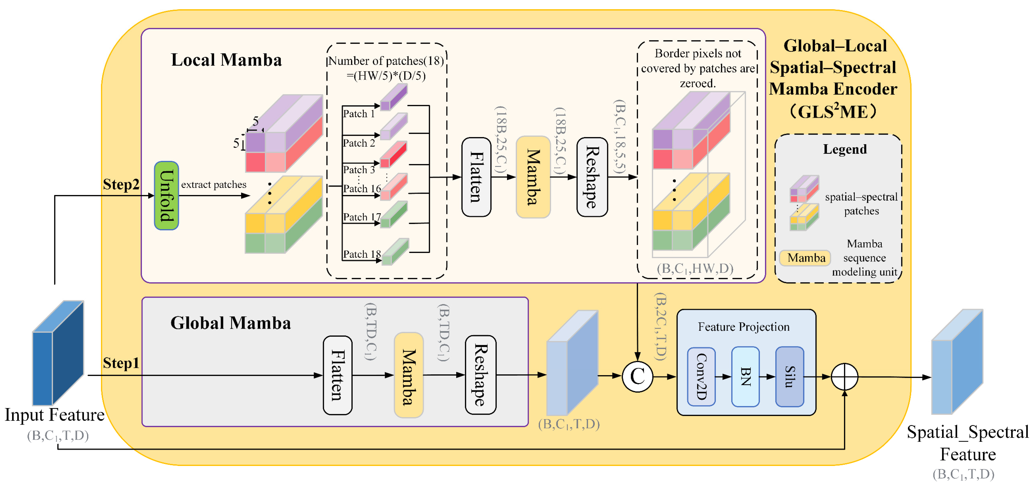
To capture both the global contextual semantics and local spatial–spectral details, we propose a Global–Local Spatial–Spectral Mamba Encoder (GLS2ME) designed for comprehensive global–local spatial–spectral feature extraction. The overall workflow is illustrated in Figure 2, and the concrete steps are as follows:
Figure 2. Flowchart of the Global–Local Spatial–Spectral Mamba Encoder (GLS2ME). Step 1 (Global Mamba): the full input is flattened/serialized (Flatten) into a sequence and passed through the Global Mamba block to capture long-range spatial–spectral dependencies. Step 2 (Local Mamba): the input is also partitioned by an Unfold (sliding-window) operation into spatial–spectral patches. Each patch is serialized (Flatten) and processed by Local Mamba to preserve fine-grained local spatial–spectral structure (Border pixels not covered by patches are zeroed). The Local and Global outputs are fused and passed through a feature-projection block to produce the final spatial–spectral feature map. Finally, a residual skip connection adds the original input to the fused output to preserve low-level information and stabilize optimization.
  • Step 1: The output features from the embedding layer are fed into the global path (as illustrated by the Global Mamba in Figure 2). The features are first flattened along the spatial dimension to form a sequence, which is then processed by the global Mamba to capture long-range dependencies across both spatial and spectral domains. The resulting features are subsequently reshaped back to the original spatial structure to preserve the integrity of discriminative patterns and structural consistency. Let the pixel-level embeddings be denoted as H R B × C 1 × T × D 1 ; the specific computation is listed as follows:
H ( seq ) =   Flatten   H H g = Mamba glob   H ( seq )   H g = Reshape H ( g )  
where H ( seq ) R B × T D 1 × C 1 , H g R B × T D 1 × C 1 . Flatten   · maps the spatial dimensions S × S into a sequence of length S 2 , Reshape · performs the inverse operation. Mamba glob   ·  denotes the Mamba unit used for global modeling. Through these operations, the network can fully extract global spatial–spectral features.
  • Step 2: The output features from the embedding layer are fed into the local path (as illustrated by the Local Mamba in Figure 2). First, the input is divided into multiple non-overlapping local patches P k k = 1 N (in this work N = 18 ) of size w × w (in this work w = 5 ). Each patch is then flattened within the patch and processed by the local Mamba to model intra-patch dependencies, resulting in P k R B × N × w w × C 1 (where N = T p + D 1 p , T p = T w , D 1 p = D 1 w , w w = w × w ). If the spatial dimension T or the spectral dimension D 1 is not divisible by the window size w , the edge pixels that are not fully covered are excluded from local path computation; their positions in the local feature map are set to zero (As shown by the final scatter-add operation in the Local Mamba in Figure 2) and subsequently compensated by the global path and residual connections. After processing, each patch is restored to its original spatial location, and overlapping regions (if any) are averaged to produce the final local feature map. The detailed procedure is listed as follows:
P k ( flat ) = Flatten _ patch P k P ˜ k = Mamba loc   P k ( flat ) H l = Reconstruct ( P k k = 1 N )
where P k ( flat ) , P ˜ k R B N × w w × C 1 ( B N = B × N ), H l R B × C 1 × T × D 1 . Mamba loc   · denotes the Mamba unit employed for modeling within local windows. Reconstruct ( · )  denotes the operation that reassembles processed patch outputs into their original spatial locations and, where patches overlap, averages overlapping values by the number of contributions; in the non-overlapping case, this operation reduces to direct placement of each processed patch (As shown in the scatter add part in Figure 2). Although pure global serialization facilitates long-distance modeling, the flattening and scanning procedures can disrupt the spatial coherence of the central pixel and dilute local details, thereby weakening discrimination for small targets, edges, and fine texture structures. Introducing a local path preserves the local neighborhood structure and enables modeling of fine-grained spatial–spectral dependencies within patches using much shorter sequence lengths. This design both compensates for the global Mamba’s limited sensitivity to local detail and substantially reduces the computational and memory costs of local sequences, which in turn facilitates parallel processing and fusion.
  • Step 3: The global and local features are concatenated along the channel dimension, projected by a 1 × 1 convolution, and then processed by batch normalization and a nonlinear activation to form the fused representation. The fused representation is subsequently added to the input via a residual connection to achieve integration of global and local features. The detailed structure is shown in the remaining parts of Figure 2. The fusion process is listed as follows:
H cat   = Concat H g , H l H p = SiLU BN Conv 1 × 1 H cat
where H cat   R B × 2 C 1 × T × D 1 , H p R B × C 1 × T × D 1 . Conv 1 × 1 ( · ) denotes a per-channel linear projection, and the final output is produced using a residual connection:
H spa _ spe = H + H p
where H spa _ spe R B × C 1 × T × D 1 . To achieve a full integration of spatial and spectral features through the above operations. The proposed method employs a global path to model long-range spatial–spectral dependencies, while a local path extracts local features through non-overlapping sliding windows, modeling short-range relationships within small patches. The two feature streams are then integrated via a Feature Projection module and refined through a residual feedback connection. In hyperspectral imagery, class-discriminative information typically manifests as a highly coupled pattern between spatial and spectral domains. On one hand, the same material exhibits consistent spectral responses across several adjacent bands; on the other hand, these responses show structured spatial distributions, such as texture regularity, boundary continuity, and local neighborhood consistency. Based on this observation, each spatial–spectral position in the hyperspectral cube is treated as a joint grid point, enabling the network to learn cross-dimensional dependencies directly within the product domain of space and spectrum. This joint modeling strategy avoids the limitations of separate spatial and spectral modeling, thus enhancing information interaction and feature fusion.

2.6. Hierarchical Spectral Mamba Encoder

To characterize spectral-shape differences at multiple scales along the spectral dimension and to explore group-level inter-band relationships while maintaining controllable computational cost, this study proposes the Hierarchical Spectral Mamba Encoder (HSME). For each spatial location, the method applies multi-receptive-field 1D convolutions to obtain multi-scale spectral responses. The multi-scale responses are concatenated along the channel dimension and, following a grouping strategy, fed into Mamba encoders to model inter-group dependencies. Finally, the outputs are reconstructed and fused with residual connections to recover discriminative spectral representations, as illustrated in Figure 3. The concrete steps are as detailed below.
Figure 3. Flowchart of the Hierarchical Spectral Mamba Encoder (HSME). The input features are first flattened and passed through three parallel 1D convolutions at different receptive scales. The resulting feature maps are concatenated and reshaped into a token sequence for a Mamba sequence operator, which models long-range spectral dependencies. The processed sequence is then reshaped into the target layout required by the subsequent layers, followed by group normalization and a SiLU activation. Finally, a residual skip connection adds the original input features to the processed output to preserve low-level information and stabilize optimization.
  • Step 1: Let H denote the input data. Three 1D convolutions with different receptive fields are applied to extract spectral responses at fine, medium, and coarse scales, respectively.
M 3 = Conv k = 3 ( H ) M 7 = Conv k = 7 ( H ) M 11 = Conv k = 11 ( H )
where M 3 , M 7 , M 11 R J × 1 × C 1 ( J = B × T × D 1 ). And Conv k = 3 , Conv k = 7 , Conv k = 11  denote 1D spectral convolutions with kernel sizes 3, 7, and 11, respectively. The three responses are concatenated along the channel dimension to obtain the multi-scale spectral representation:
H ms = Concat M 3 , M 7 , M 11
where H ms R J × 3 × C 1 . For subsequent group-level (token) modeling, a tokenization strategy is applied to divide H ms into K tokens (here K = 4 ). Zero-padding is applied along the channel dimension if necessary to ensure divisibility or to match the predefined group channel number M , and H pad denotes the padded result. Let each token contain M  channels after grouping, then:
H pad = PadTo H ms , T M , X flat   = Group H pad   ; T
where Group ; T denotes the operation that rearranges the channel dimension into K tokens, producing the group-level token sequence X flat   R J × K × 3 C 1 K .
  • Step 2: The Mamba-based group-level feature extraction models semantic relationships among groups along the token dimension.
Y flat = Mamba X flat
This operation enables interactions among different spectral groups to be captured, thereby enhancing the discriminability of spectral vectors. Mamba ·  denotes the Mamba unit used in this work, which is responsible for information exchange and representation updating among group-level tokens.
  • Step 3: The output of Mamba is reconstructed according to the channel layout to form a multi-scale channel representation, and its expressive capacity is further enhanced through normalization and activation.
H recon = SiLU ( GN ( Reshape ( Y flat ) ) )
where H recon R B × 3 C 1 × T × D 1 , and GN ·  denotes Group Normalization. Residual fusion is employed to preserve the original spectral information and improve training stability:
H spe = H + P H recon
where H spe R B × C 1 × T × D 1 , and P · denotes taking the first C 1  channels of the reconstructed result when necessary. Through all the above steps, the goal of fully capturing spectral features of hyperspectral images at different scales is achieved.

2.7. Feature Fusion Module

We use a Feature Fusion Module [33] to jointly model spatial–spectral features. Its residual connections reduce gradient vanishing and speed up convergence, and via identity mapping they guide the network to learn useful incremental features instead of overfitting noise on small samples, improving generalization (purple block in Figure 1b).

2.8. Progressive Residual Fusion Block

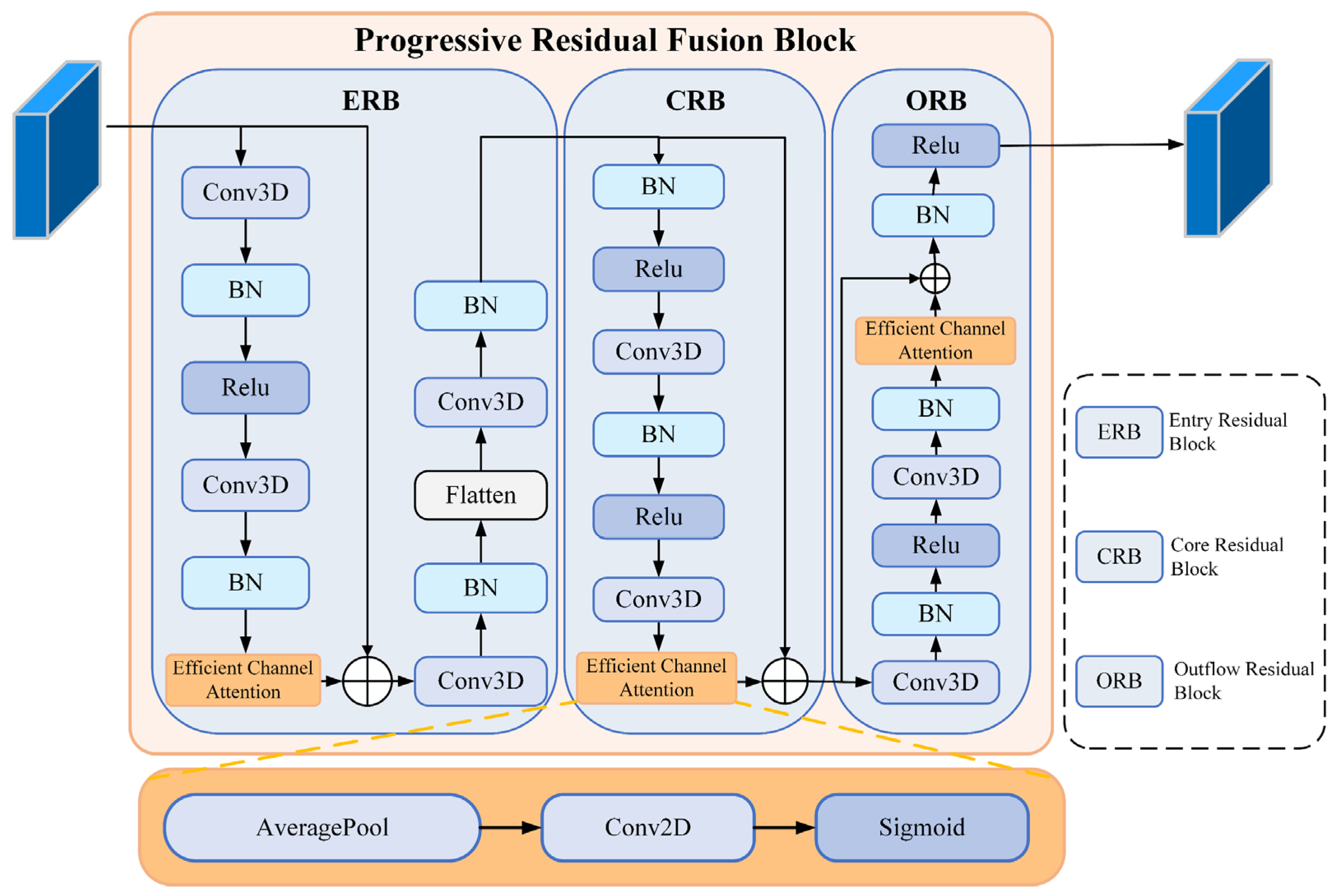
We propose the Progressive Residual Fusion Block (PRFB) to fuse multi-scale spatial–spectral features from the Mamba encoders into the classifier. In the PRFB, we adopt the Efficient Channel Attention (ECA) [34] mechanism to capture long-range and non-linear inter-channel dependencies within feature maps, thereby enhancing spectral discriminability (see the orange block in Figure 4 Efficient Channel Attention). PRFB uses progressive enhancement and multi-scale residual fusion to suppress redundant information, amplify discriminative channels, remain parameter- and computation-compact, and improve generalization in few-shot and class-imbalanced scenarios. Steps are shown in Figure 4:
Figure 4. Flowchart of the Progressive Residual Fusion Block (PRFB). The PRFB comprises three sequential submodules. Entry Residual Block (ERB), which transforms the input into a compact multi-scale spatial–spectral representation that preserves fine detail and suppresses noise, performs channel expansion, spectral aggregation, cross-axis reordering, and spatial-spectral downsampling. Core Residual Block (CRB), a stack of residual stages, progressively extracts deeper spatial-spectral features and improves channel discrimination. Outflow Residual Block (ORB) acts as a feature organizer and stabilizer, ensuring the output exhibits stable statistical distributions and well-separated decision boundaries prior to pooling and classification. Each submodule includes an Efficient Channel Attention (ECA) unit for channel recalibration.
  • Step 1 (Entry Residual Block): The ERB transforms the input into a compact, multi-scale spatial–spectral representation that preserves fine detail and suppresses noise. It expands channels with a convolution, aggregates along the spectral axis, reorders feature axes for cross-axis interaction, applies a second convolution, and concludes with spatial and spectral downsampling (see Figure 4 ERB)
X 1 = F ERB ( X pre ) = F k ( Flatten ( F k ( X pre + F ECA ( F k ( ReLU ( F k ( X pre ) ) ) ) ) ) )
where X 1 R B × C × S 1 × S 1 × D 1 ( S 1 denotes the transformed spatial dimensions (width and height) of the data after convolution), F ECA ( · ) denotes Efficient Channel Attention (ECA) module, F k denotes BN ( Conv ( · ) ) , Conv ( · )  denotes 3D convolution. The above steps provide a smooth transition from the raw data to the deep network; these steps suppress noise and enhance early discriminative features while preserving spectral integrity.
S 1 denotes the spatial dimensions after convolution; F ECA ( · ) is the Efficient Channel Attention (ECA) module; F k denotes BN ( Conv ( · ) ) ; Conv ( · )  denotes a 3D convolution. These preprocessing steps provide a smooth transition from raw data into the deep network, suppressing noise and enhancing early discriminative features while preserving spectral integrity.
  • Step 2 (Core Residual Block): A stack of 3D convolutions with residual links progressively extracts deeper spatial–spectral features and improves channel discrimination (see Figure 4 CRB):
X 2 = F CRB ( X 1 ) = X 1 + F ECA ( F k 1 ( F k 1 ( X 1 ) ) )
where X 2 R B × C × S 1 × S 1 × D 1 . F k 1 denotes Conv ( ReLU ( BN ( · ) ) ) .
  • Step 3 (Outflow Residual Block): The ORB serves as a feature organizer and stabilizer, ensuring that the output features exhibit stable statistical distributions and well-separated decision boundaries before the pooling and fully connected stages (see Figure 4 ORB):
X 3 = ( F CRB ( X 2 ) = ReLU ( BN ( X 2 + F ECA ( F k 1 ( F k 1 ( X 2 ) ) ) ) ) )
where X 3 R B × C × S 1 × S 1 × D 1 .

3. Experimental Details

To validate the effectiveness of the proposed S2GL-MambaResNet network, comparative experiments were conducted on three classical public hyperspectral datasets and one double-high (H2) dataset, including visualized classification results, ablation studies, parameter analysis, sample-sensitivity verification, and computational-complexity analysis. The classification results are shown from Tables 6–9. All experiments were performed on a computing platform equipped with an RTX 4090D GPU (24 GB memory) and 80 GB RAM. This section first introduces the datasets used, then provides the experimental parameter settings and comparison methods, and finally analyzes the experimental results.

3.1. Dataset Description

To systematically evaluate the adaptability and classification performance of the proposed S2GL-MambaResNet across different sensors and various scene conditions, four representative datasets were selected: Botswana, Salinas, Houston2013 (used to validate classification performance in typical hyperspectral scenarios), and WHU-Hi-LongKou [35] (used to test classification performance at H2 dataset). These four datasets were acquired by different sensors under diverse environmental conditions and thus collectively reflect the network’s classification performance under varying imaging conditions. Table 1 provides a brief description of the four datasets, and Table 2, Table 3, Table 4 and Table 5 list their training and testing splits.
Table 1. Dataset-related description. This table lists the size of each dataset (pixels, width × length), the number of spectral bands (Bands), spatial resolution (m) and spectral range (nm), sensor name, and the training/test sample ratios used in our experiments. Manufacturer, city, and country of the sensors are: Hyperion—Northrop Grumman (originally TRW), Redondo Beach, CA, USA; CASI-1500—ITRES Research Ltd., Calgary, Canada; AVIRIS—NASA Jet Propulsion Laboratory (JPL), Pasadena, CA, USA; DJI Matrice 600 Pro—SZ DJI Technology Co., Ltd. (DJI), Shenzhen, China.
Table 2. Category information for Botswana dataset. Train and Test show the number of labeled pixels used for training and testing, respectively.
Table 3. Category information for Houston2013 dataset. Train and Test show the number of labeled pixels used for training and testing, respectively.
Table 4. Category information for Salinas dataset. Train and Test show the number of labeled pixels used for training and testing, respectively.
Table 5. Category information for WHU-Hi-LongKou dataset. Train and Test show the number of labeled pixels used for training and testing, respectively.

3.2. Experimental Parameter Settings

During training, the S2GL-MambaResNet was optimized using the Adam optimizer with a batch size of 16. Training was performed for 200 epochs with a learning rate of 0.0001. For all four hyperspectral datasets, image patches of size 7 × 7 were used. Each experiment was repeated 10 times, and all evaluation metrics are reported as mean ± standard deviation.

3.3. Comparison Methods

To evaluate the classification performance of S2GL-MambaResNet, we compared it with nine state-of-the-art methods: two CNN-based methods (SSRN [36], A2S2K-ResNet [37]), two GCN-based methods (GTFN [38], H2-CHGN [39]), two Transformer-based methods (SSFTT [40], GSC_ViT [41]), and three SSM-based methods (MambaHSI [33], IGroupSS-Mamba [24], S2Mamba [42]). All competing methods were configured using the default parameter settings reported in their respective references; for detailed parameter configurations and implementation details, refer to the cited literature.

3.4. Quantitative Experimental Results

3.4.1. Comparison of Classification Metrics

Table 6 presents the classification results of different networks on the Botswana dataset. As shown in Table 6, the proposed S2GL-MambaResNet achieves the best overall performance: OA = 98.88 ± 0.64%, AA = 98.91 ± 0.66%, and Kappa = 98.78 ± 0.70, demonstrating clear superiority and effectiveness. Specifically, the OA of S2GL-MambaResNet is higher than those of the CNN-based methods SSRN and A2S2K-ResNet by 2.84% and 2.58%, respectively; higher than the GCN-based methods GTFN and H2-CHGH by 1.97% and 1.70%, respectively; higher than the Transformer-based methods SSFTT and GSC_ViT by 5.25% and 1.21%, respectively; and higher than the SSM-based methods MambaHSI, IGroupSS-Mamba, and S2Mamba by 1.08%, 2.03%, and 20.58%, respectively. Compared with the first two SSM-based methods, S2GL-MambaResNet can extract both fine-grained and global spectral features via the Hierarchical Spectral Mamba Encoder, thereby enhancing the discriminability of spectral features; furthermore, the Global_Local Spatial_Spectral Mamba Encoder enables collaborative representation of local textures and global context, effectively capturing spatial context and the intrinsic continuity of spectral sequences. As for S2Mamba, its OA is the lowest among the compared networks, mainly because it introduces a large number of learnable sequence-modeling parameters for each channel and position (high capacity and non-shared) and employs gated fusion with hard thresholds. Under limited-sample conditions, these sensitive sequence and scale parameters are difficult to estimate stably and are prone to fitting training noise as signal, which leads to numerical instability, overfitting, and degraded classification accuracy. By contrast, the proposed PRFB preserves the original local spatial–spectral information; even if Mamba’s gating or complex transformation outputs are abnormal, the network does not lose key signals. Consequently, under scarce-sample conditions, the network still achieves feature enhancement, information preservation, and robust generalization, avoiding overfitting.
Table 6. OA, AA and Kappa values on the Botswana dataset using a fixed 4% training set. Results are reported as mean ± standard deviation, where ±denotes the between-run standard deviation, computed over 10 independent runs. The best result in each row is highlighted in bold.
Table 7 presents the results of different methods on the Houston2013 dataset. This dataset contains a large number of pixels and a complex land-cover distribution, which increases the difficulty of classification. Despite these challenges, the proposed S2GL-MambaResNet achieves the best overall performance: OA = 82.25 ± 1.07%, AA = 83.79 ± 0.67%, and Kappa = 80.83 ± 1.16, demonstrating clear superiority and effectiveness. Taking the Kappa coefficient as an example, S2GL-MambaResNet surpasses SSRN by 7.00, A2S2K-ResNet by 6.84, GTFN by 7.10, H2-CHGN by 4.34, SSFTT by 5.05, GSC_ViT by 3.06, MambaHSI by 1.52, IGroupSS-Mamba by 4.25, and S2Mamba by 35.68. These results demonstrate the advantage of S2GL-MambaResNet and its capability to handle complex data.
Table 7. OA, AA and Kappa values on the Houston2013 dataset using a fixed 0.5% training set. Results are reported as mean ± standard deviation, where ±denotes the between-run standard deviation, computed over 10 independent runs. The best result in each row is highlighted in bold.
Moreover, S2GL-MambaResNet achieves the highest class accuracy (CA) in four classes, more than any competing method, further confirming its effectiveness in scenarios with limited samples and class imbalance. In particular, the network shows pronounced advantages for class 1 (“Grass_healthy”), class 2 (“Grass_stressed”), and class 3 (“Grass_synthetic”). For this case, the main reason is that the relevant classes are spatially adjacent and have highly similar visual and spectral representations, which substantially increases inter-class discrimination difficulty. By extracting and fusing both global and local spatial–spectral features, S2GL-MambaResNet captures richer spatial textures and spectral details across scales, enabling more accurate discrimination of these neighboring, spectrally similar classes.
Table 8 presents the results of different methods on the Salinas dataset. As shown in Table 8, S2GL-MambaResNet achieves the best overall performance: OA = 94.84 ± 0.59%, AA = 96.43 ± 0.69%, and Kappa = 94.25 ± 0.66, with the lowest standard deviations for all three metrics among the compared methods. Taking the AA as an example, S2GL-MambaResNet surpasses SSRN by 10.46, A2S2K-ResNet by 4.75, GTFN by 7.12, H2-CHGN by 5.22, SSFTT by 5.11, GSC_ViT by 5.15, MambaHSI by 3.08, IGroupSS-Mamba by 3.00, and S2Mamba by 55.52. More importantly, S2GL-MambaResNet attains high class-wise accuracies across all categories; the lowest class accuracy is for class 15 (87.50%), and there is no evident collapse class (i.e., no class with near-zero or extremely low accuracy), indicating that S2GL-MambaResNet exhibits strong stability and generalization under scarce-sample conditions. By contrast, although some methods (e.g., MambaHSI) achieve the highest accuracy in several individual classes (as visible in the table), they suffer from pronounced performance drops in other classes. For example, MambaHSI achieves only 70.21% and 75.34% for classes 3 and 10, respectively, which indicates a risk of severe class imbalance sensitivity and fragility when training samples are extremely limited. A closer inspection of the per-class results in Table 8 shows that some methods exhibit large class-wise variances or near-zero accuracies in several classes. For instance, SSRN shows class standard deviations greater than 20% for classes 4, 5, 12, and 14, and A2S2K-ResNet reports standard deviations exceeding 30% for classes 5 and 12. More critically, S2Mamba demonstrates near-collapse behavior in multiple classes (classes 1, 3, 11, and 16: 0.00 ± 0.00%; classes 12, 14, and 15: 4.39%, 3.63%, and 1.55%, respectively), indicating that this method fails to robustly learn discriminative features for these land-cover types under extremely limited training samples. These observations further corroborate the superiority of S2GL-MambaResNet in few-shot and imbalance scenarios.
Table 8. OA, AA and Kappa values on the Salinas dataset using a fixed 0.15% training set. Results are reported as mean ± standard deviation, where ±denotes the between-run standard deviation, computed over 10 independent runs. The best result in each row is highlighted in bold.
Table 9 presents the results of different methods on the WHU-Hi-LongKou dataset. It is important to emphasize that WHU-Hi-LongKou is the only H2 dataset in our experiments; therefore, it imposes higher demands on a network’s ability to simultaneously capture spectral details and spatial textures. Under few-shot conditions, S2GL-MambaResNet achieves a clear advantage in overall metrics: OA = 95.34 ± 0.88%, AA = 90.22 ± 1.97%, Kappa = 93.85 ± 1.17, outperforming most competing methods in the table—for example, it improves OA by approximately 1.37% relative to the second-best method (GSC_ViT). The relatively small overall standard deviations indicate that the results are both superior and stable. Per-class analysis further highlights the robustness of S2GL-MambaResNet in H2 scenarios: it maintains high accuracies across all nine classes (the lowest being class 2 at 81.98 ± 10.49%; most other classes are near or above 85%), with no collapse classes. By contrast, several competing methods fail catastrophically on some classes: for instance, S2Mamba yields only 0.00 ± 0.00%, 0.01 ± 0.01%, and 0.41 ± 0.41% for classes 3, 5, and 9, respectively (practically unrecognizable), whereas S2GL-MambaResNet attains 87.20 ± 16.28%, 86.27 ± 9.22%, and 86.53 ± 8.81% on the same classes—differences that are highly significant. Similarly, although MambaHSI achieves very high accuracy for class 1 (99.29%), it performs poorly for classes 8 and 9 (50.05% and 67.84%, respectively), indicating an imbalanced performance under H2 few-shot conditions. In contrast, S2GL-MambaResNet tends to produce high and more uniform per-class accuracies, which yields higher OA, AA, and Kappa values and lower standard deviations overall.
Table 9. OA, AA and Kappa values on the WHU-Hi-LongKou dataset using a fixed 0.04% training set. Results are reported as mean ± standard deviation, where ±denotes the between-run standard deviation, computed over 10 independent runs. The best result in each row is highlighted in bold.

3.4.2. Comparison of Classification Maps

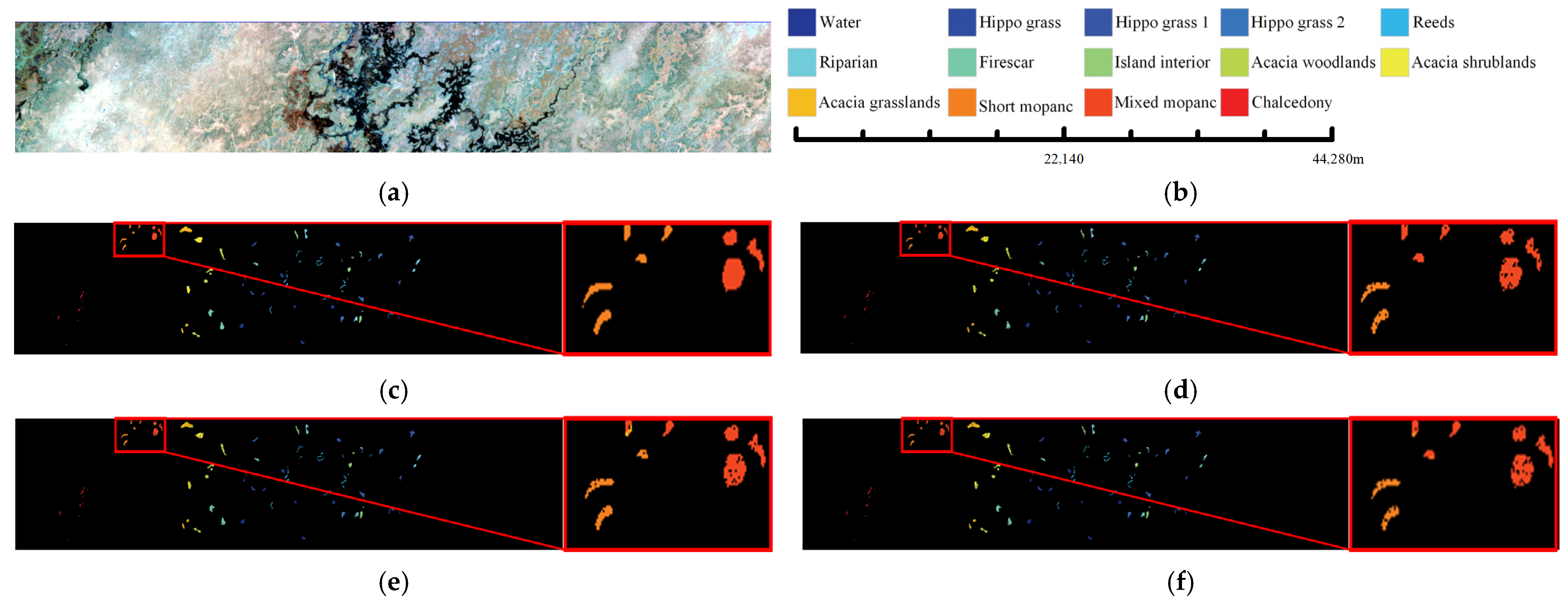
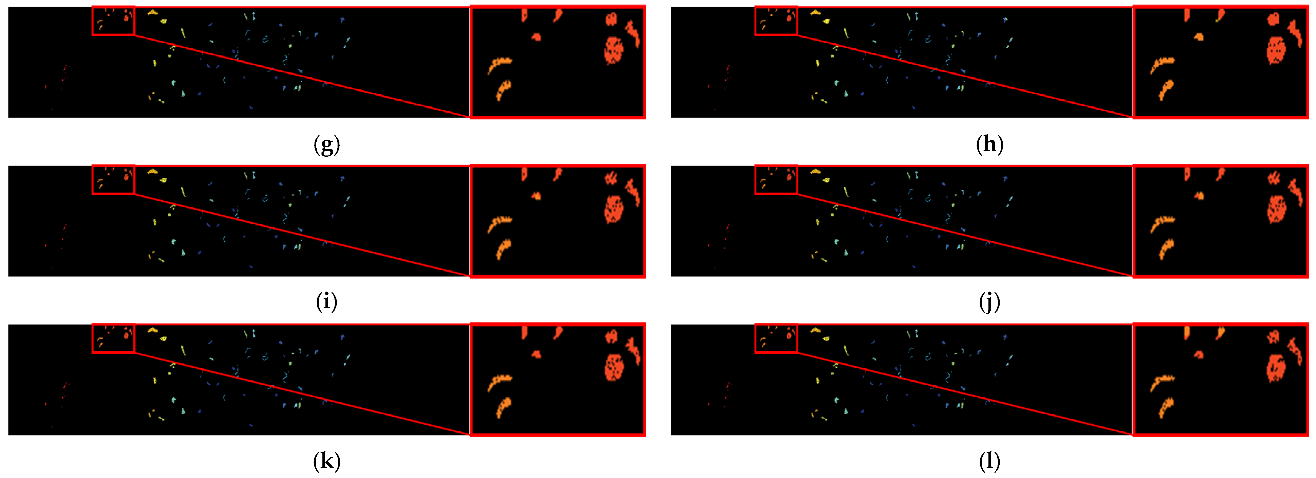
The classification maps are compared to further validate the effectiveness of S2GL-MambaResNet. Figure 5, Figure 6, Figure 7 and Figure 8 present the classification results of the proposed method on the four datasets. To make the differences among the methods more visually distinguishable, selected subregions of the images are enlarged.
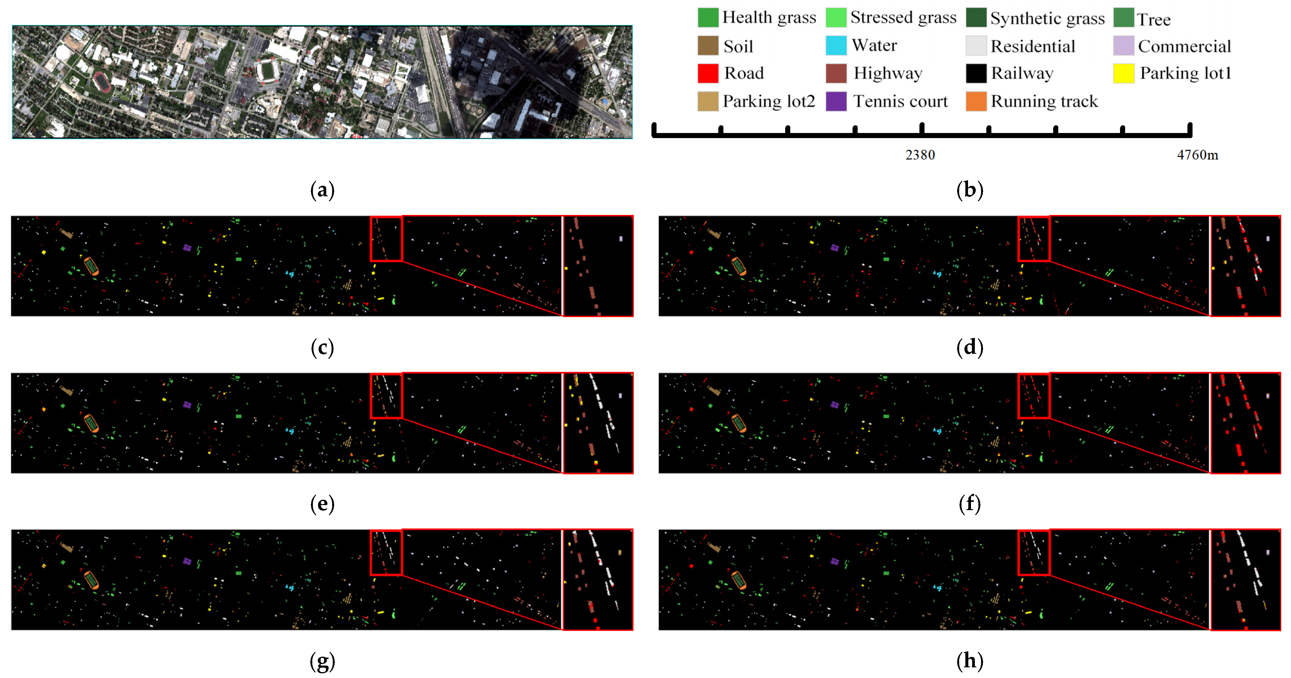
Figure 5. Classification maps for the Botswana image. (a) False composite map. (b) Legends and scale bar. (c) Ground-truth map. (dl) Classification maps of SSRN, A2S2K-ResNet, GTFN, H2-CHGN, SSFTT, GSC_ViT, MambaHSI, IGroupSS-Mamba, and our S2GL-MambaResNet.
Figure 6. Classification maps for the Houston2013 image. (a) False composite map. (b) Legends and scale bar. (c) Ground-truth map. (dl) Classification maps of SSRN, A2S2K-ResNet, GTFN, H2-CHGN, SSFTT, GSC_ViT, MambaHSI, IGroupSS-Mamba, and our S2GL-MambaResNet.
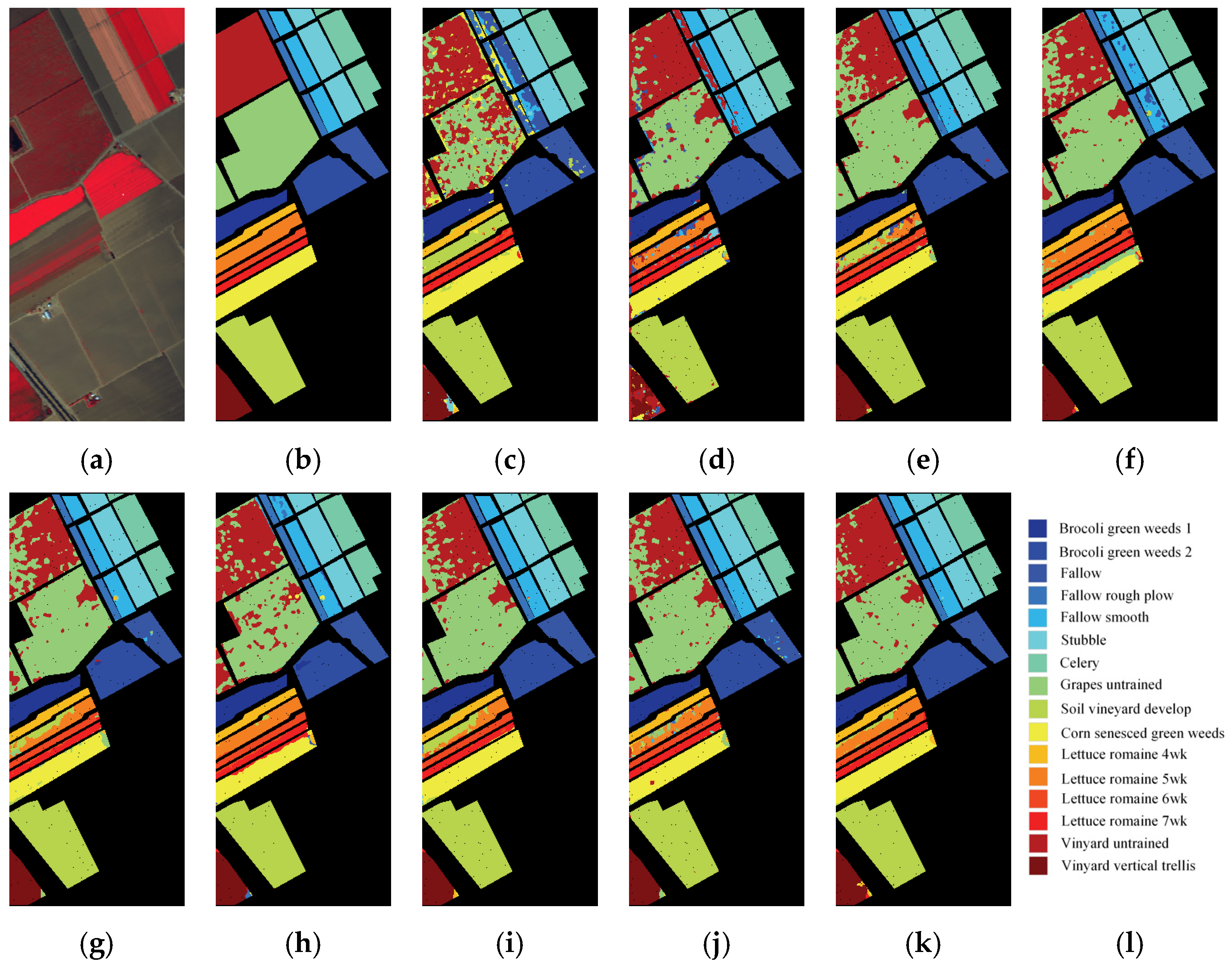
Figure 7. Classification maps for the Salinas image. (a) False composite map. (b) Ground-truth map. (ck) Classification maps of SSRN, A2S2K-ResNet, GTFN, H2-CHGN, SSFTT, GSC_ViT, MambaHSI, IGroupSS-Mamba, and our S2GL-MambaResNet. (l) Legends and scale bar.
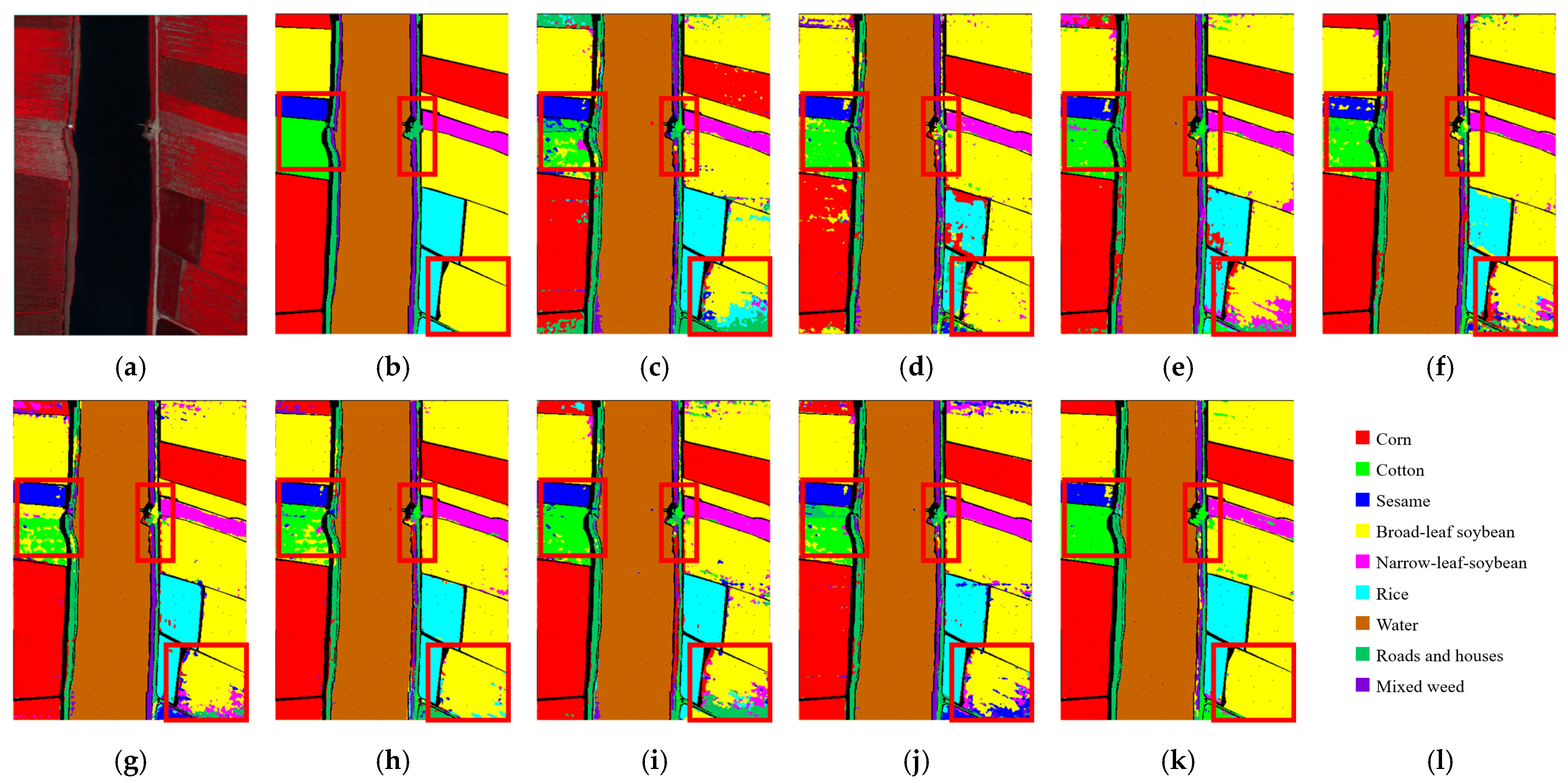
Figure 8. Classification maps for the WHU-Hi-LongKou image. (a) False composite map. (b) Ground-truth map. (ck) Classification maps of SSRN, A2S2K-ResNet, GTFN, H2-CHGN, SSFTT, GSC_ViT, MambaHSI, IGroupSS-Mamba, and our S2GL-MambaResNet. (l) Legends and scale bar.
For the Botswana dataset (Figure 5), although the targets in this scene are mostly discrete and localized, S2GL-MambaResNet still provides the most accurate prediction details. In the enlarged region, Acacia grasslands (Golden Yellow) are clearly misclassified as Mixed mopane (Orange-Red) by all other competing methods, whereas S2GL-MambaResNet yields visually improved results, showing the highest similarity to the ground truth and achieving relatively accurate classification in both smooth and boundary regions.
For the Houston2013 dataset (Figure 6), in the enlarged subregions, other methods misclassify Railway (Black) as Residential (Light Gray), Road (Red), Highway (Reddish Brown), and Parking lot 1 (Yellow). Similarly, Highway is often confused with Road and Parking lot 1. These classes exhibit similar linear and elongated structures with strong connectivity and orientation, making them challenging to distinguish. In contrast, S2GL-MambaResNet leverages multi-scale spatial context modeling and spatial–spectral joint representation to better preserve the elongated continuity and textural cues of these ground objects. This significantly reduces mutual confusion among these classes in both smooth and boundary areas, resulting in improved classification performance.
For the Salinas dataset (Figure 7), which mainly consists of agricultural categories with high spectral similarity, intra-class heterogeneity, and inter-class confusion, S2GL-MambaResNet demonstrates strong discriminative ability on several challenging classes. For example, other methods commonly misclassify Vinyard untrained (Deep Red) as Grapes untrained (Light Green) and Lettuce romaine 4 wk (Bright Golden Yellow) as Soil vineyard develop (Lime Green). These misclassifications mainly arise because (1) Vinyard untrained and Grapes untrained have highly similar reflectance in the visible–near-infrared region, especially during the early growth stage or under low canopy cover; and (2) mixed-pixel effects and bare soil influence cause boundary and sparse vegetation pixels to exhibit mixed spectral signatures, increasing confusion between Lettuce romaine 4 wk and Soil vineyard develop. In contrast, S2GL-MambaResNet produces more accurate classification maps, indicating that its spatial–spectral joint modeling and multi-scale contextual aggregation enhance both overall recognition accuracy and the ability to discriminate spectrally similar crop types.
For the WHU-Hi-LongKou dataset (Figure 8), the red box highlights that most competing methods show obvious confusion among Cotton (Pure Green), Sesame (Pure Blue), Broad-leaf soybean (Yellow), Narrow-leaf soybean (Magenta), and Mixed weed (Deep Purple). As an H2 dataset in the WHU-Hi series, WHU-Hi-LongKou provides both rich spectral information and fine-grained field textures. From a spectral perspective, these crop types often exhibit overlapping reflectance curves in the visible–NIR range (especially when canopy coverage, water content, or growth stages are similar), making spectral-only classification prone to errors. Additionally, soil background, shadows, and irrigation-induced variations increase intra-class variability. From a spatial perspective, the high spatial resolution enables observation of fine structures such as field row patterns, plant spacing, and crop strip textures. However, when canopy cover is sparse or field plots are small (e.g., narrow-leaf soybean rows or mixed weeds), these spatial signals may be weakened by noise, bare soil between rows, or geometric distortions, making it difficult for single-scale or weak spatial modeling methods to accurately distinguish similar classes. The classification maps produced by S2GL-MambaResNet display more continuous and smooth field boundaries, fewer isolated noisy patches, and more consistent intra-class regions, demonstrating its superior ability to preserve field strip textures and suppress mixed-pixel effects.

3.5. Ablation Experiments

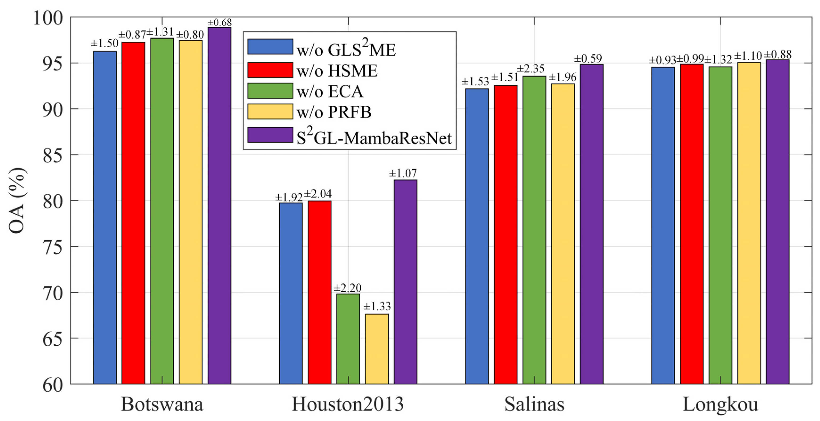
To further evaluate the contribution of each component within S2GL-MambaResNet, ablation experiments were conducted while keeping all other experimental settings unchanged (shown in Figure 9).
Figure 9. Ablation comparison of each variant in S2GL-MambaResNet. Bar plots show overall accuracy (OA, %) for different ablation variants (w/o GLS2ME, w/o HSME, w/o ECA, w/o PRFB) and the full S2GL-MambaResNet across four datasets (Botswana, Houston2013, Salinas, WHU-Hi-LongKou). Results are reported as mean ± standard deviation, where ±denotes the between-run standard deviation computed over 10 independent runs and annotated on the bars.
(1)
w/o GLS2ME: The Global_Local Spatial_Spectral Mamba Encoder was removed from S2GL-MambaResNet.
(2)
w/o HSME: The Hierarchical Spectral Mamba Encoder was removed.
(3)
w/o ECA: The Efficient Channel Attention within the Progressive Residual Fusion Block was removed.
(4)
w/o PRFB: Both the Efficient Channel Attention and the residual summation within the Progressive Residual Fusion Block were removed.
These four variants were then applied to the Botswana, Salinas, Houston2013, and WHU-Hi-LongKou datasets for classification. Each module ablation experiment was repeated 10 times, and the Overall Accuracy (OA) with mean ± standard deviation was used as the evaluation metric (the standard deviation is annotated above each bar in Figure 9). Figure 9 presents the bar charts of OA scores on the four hyperspectral datasets, where different colors correspond to different variants and the original S2GL-MambaResNet is shown in purple. It is evident that the purple bars are consistently the highest, indicating that removing any of these components leads to a significant drop in OA. Since the four datasets cover different types of scenes, the degree of performance degradation varies across components. On the Houston2013 dataset, the green (w/o ECA) and yellow (w/o PRFB) bars are the lowest. Specifically, removing ECA substantially reduces the model’s ability to capture fine-grained spatial–spectral discriminative cues in urban-scale hyperspectral imagery. For w/o PRFB, the accuracy drop is the most severe because both the ECA and residual connections are removed, leading to feature attenuation and hindered gradient flow in deeper layers. This is particularly detrimental for complex datasets such as Houston2013, where the land-cover types are spatially scattered and exhibit relatively small inter-class spectral differences. Overall, GLS2ME has the greatest impact on classification accuracy, as the blue bars (w/o GLS2ME) are the lowest in three of the datasets.
As for standard deviation, the observed standard deviations are small overall, with a maximum of 2.35%, indicating low run-to-run variability and good experimental repeatability. Averaging across the four datasets, the mean standard deviations for the four ablation variants are: w/o PRFB: 1.30%, w/o ECA: 1.80%, w/o GLS2ME: 1.47%, and w/o HSME: 1.35%. These values show that the measured OA differences are consistent across repeated trials and not dominated by random fluctuation. From the dataset perspective, Salinas exhibits the largest sensitivity to module removal: the OA range across variants on Salinas is 13.93% (68.13% → 82.06%), and its mean standard deviation is 1.87%, both of which are higher than those of the other datasets. Botswana and WHU-Hi-LongKou are the most stable, with OA ranges of 2.29% and 0.98%, and mean standard deviations of 1.12% and 1.08%, respectively. Houston2013 shows moderate variability (OA range 4.03%, mean std 1.84%), consistent with its more complex urban spatial patterns. Importantly, the performance drops caused by removing each component are generally much larger than the corresponding standard deviations, which supports the interpretation that the observed degradations are systematic and attributable to the ablated modules rather than to experimental noise.
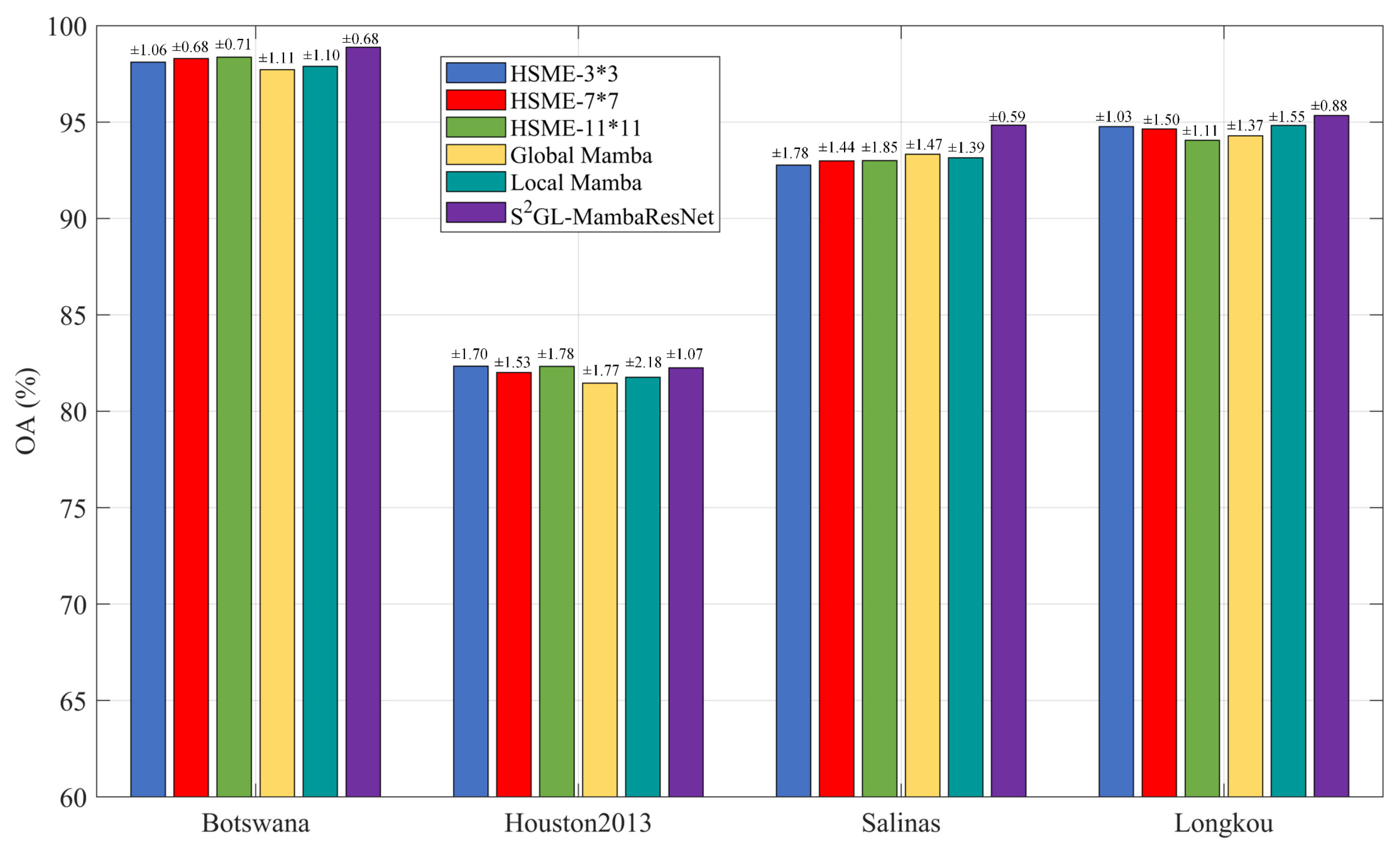
To provide a finer-grained comparison of the contributions of the global and local paths in GLS2ME and the convolutional kernels of different scales in HSME, we conducted detailed ablation studies on these two modules (see Figure 10). Each ablated variant was evaluated over 10 independent runs, with the results reported as mean ± standard deviation (the standard deviation is annotated above each bar in Figure 10).
Figure 10. Fine-Grained Ablation Study of Global–Local Spatial–Spectral Mamba Encoder (GLS2ME) and Hierarchical Spectral Mamba Encoder (HSME). Bar plots show overall accuracy (OA, %) for the evaluated variants (HSME-3*3, HSME-7*7, HSME-11*11, Global Mamba, Local Mamba, the * denotes multiplication) and the full S2GL-MambaResNet across four datasets (Botswana, Houston2013, Salinas, WHU-Hi-LongKou). Results are reported as mean ± standard deviation, where ±denotes the between-run standard deviation computed over 10 independent runs and annotated on the bars.
(1)
HSME-3*3: Only the 3*3 small-scale convolutional kernels were used in the HSME.
(2)
HSME-7*7: Only the 7*7 medium-scale convolutional kernels were used in the HSME.
(3)
HSME-11*11: Only the 11*11 large-scale convolutional kernels were used in the HSME.
(4)
Global Mamba: Only the global path was retained in the GLS2ME.
(5)
Local Mamba: Only the local path was retained in the GLS2ME.
On the Botswana and Houston2013 datasets, HSME-11*11 achieved the highest accuracy compared to the other ablation variants, indicating that large-scale spectral context is crucial for scenes containing extensive homogeneous areas or complex artificial features. On the Salinas dataset, the three kernel sizes performed comparably, with only minor differences in OA. On the WHU-Hi-LongKou dataset, HSME-3*3 (94.76%) and HSME-7*7 outperformed HSME-11*11, suggesting that excessively large kernels may introduce unnecessary spectral noise in such scenarios. Global Mamba achieved higher OA than Local Mamba on three datasets (Botswana, Houston2013, and WHU-Hi-LongKou), with a particularly notable advantage on WHU-Hi-LongKou. This demonstrates that local detail features are critically important for classifying dual-high-resolution agricultural scenes. In contrast, Global Mamba performed best on the Salinas dataset, which can be attributed to the regular distribution of ground objects in this scene, where large-scale spatial context plays a more important role.
Regarding standard deviation, HSME-7*7 exhibited relatively low standard deviations on three of the four datasets (Botswana, Houston 2013, and Salinas), with the lowest value on Botswana (0.68%), indicating its more stable performance output. In comparison, HSME-3*3 showed a higher standard deviation of 1.70% on the Houston 2013 dataset, revealing its suboptimal stability in complex scenarios. Therefore, no single convolutional kernel size can simultaneously achieve optimal accuracy and stability across all datasets, strongly validating the necessity of the multi-scale parallel design in the original HSME module. Furthermore, on the most challenging Houston 2013 dataset, Local Mamba exhibited the largest standard deviation (2.18%), significantly higher than that of Global Mamba (1.77%) and most other variants. This indicates that relying solely on the local path leads to higher uncertainty in performance when dealing with complex urban features. In contrast, Global Mamba demonstrated moderate to low standard deviations across all datasets, reflecting its stable performance output.
In summary, the global and local paths exhibit clear functional complementarity. The global path provides stable, macro-level spatial structural information, while the local path captures fine-grained features essential for classification but may exhibit instability when used alone in complex scenes. Overall, the dual-path design of GLS2ME successfully integrates the advantages of both, enhancing both performance and model stability.

3.6. Effect of Patch Size

To evaluate the effect of patch size used in preprocessing on the classification performance of S2GL-MambaResNet, we conducted a comparison on the Botswana, Houston2013, Salinas, and WHU-Hi-LongKou datasets by increasing the patch size from 7 × 7 to 11 × 11. The results are shown in Table 10. The experiments indicate that enlarging the patch size from 7 × 7 to 11 × 11 leads to a decrease in Overall Accuracy (OA) on all four datasets to varying degrees: Botswana decreases from 98.88% to 95.22% (−3.66%); Houston2013 decreases from 82.25% to 78.53% (−3.72%); Salinas decreases from 94.84% to 89.13% (−5.71%); WHU-Hi-LongKou decreases from 95.34% to 92.28% (−3.06%). Possible reasons for the OA degradation with larger patch sizes include: (1) larger patches introduce more background redundancy and increased spectral mixing, which reduces the purity of per-pixel discriminative signals; and (2) when object/field sizes in a dataset are small or spatially dispersed, excessively large patches can over-smooth local differences and weaken the network’s ability to discriminate small-target classes. The largest drop occurs on the Salinas dataset (5.71%), suggesting the presence of fine-grained classes that are highly sensitive to background or neighborhood interference. By contrast, Longkou exhibits a smaller decline (3.06%), indicating greater within-class homogeneity or regional spectral consistency and hence greater robustness to patch-size changes. The relatively large OA fluctuation in Houston2013 implies that background redundancy and spectral mixing substantially affect classification performance on that dataset. Overall, these results suggest that smaller-scale local spatial–spectral information is more favorable for S2GL-MambaResNet; a 7 × 7 patch yields the highest OA across the four datasets.
Table 10. Sensitivity analysis for the proposed method with different sizes of input patches on the Botswana, Houston2013, Salinas, and WHU-Hi-LongKou datasets. The OA values shown are computed as the mean across 10 independent runs.

3.7. Hyper-Parameter Analysis

To evaluate the sensitivity of S2GL-MambaResNet to key hyperparameters, we conducted experiments on four datasets (Botswana, Salinas, WHU-Hi-LongKou, and Houston2013) by varying four hyperparameters independently: group number, embedding dimension, local window size, and token number. Figure 11 shows the OA obtained under each parameter setting. The main observations and their implications are as follows. Group number. Increasing the group number from 1 to 4 improves OA, further increases lead to plateauing or slight decreases. All datasets reach peak performance at Group Number = 4. Moderate grouping enables finer-grained local modeling of spectral and spatial feature components, thereby enhancing the discriminative ability of model. Token number. Token number = 4 yields the best performance. Too few tokens limit the ability to partition information and form parallel representations; too many tokens fragment information, increase computational cost, and may harm classification performance. Embedding dimension. An embedding dimension of 128 is optimal. Smaller dimensions restrict representational capacity and reduce accuracy, while excessively large dimensions can introduce redundancy or overfitting, causing OA to decrease on some datasets. Local window size. A local window size of 5 is optimal across all datasets. Windows that are too small restrict spatial–spectral contextual information, whereas overly large windows introduce background redundancy and spectral mixing, weakening discrimination of small-scale classes. The magnitude of performance degradation under extreme parameter settings varies across datasets—for example, Salinas is particularly sensitive to overly large embedding dimensions, likely due to its fine-grained classes, high within-class heterogeneity, and complex background. Taken together, the combination Group Number = 4, Token Number = 4, Embedding Dimension = 128, and Local Window Size = 5 provides sufficient representational power to capture spatial–spectral discriminative cues while avoiding excessive irrelevant information and overfitting, thereby yielding the highest OA.
Figure 11. Overall accuracy (OA) curves across four datasets under different hyperparameter configurations: (a) number of groups, (b) number of tokens, (c) embedding dimension, and (d) local window size. The OA values shown are computed as the mean across 10 independent runs.

3.8. Sample Sensitivity Verification

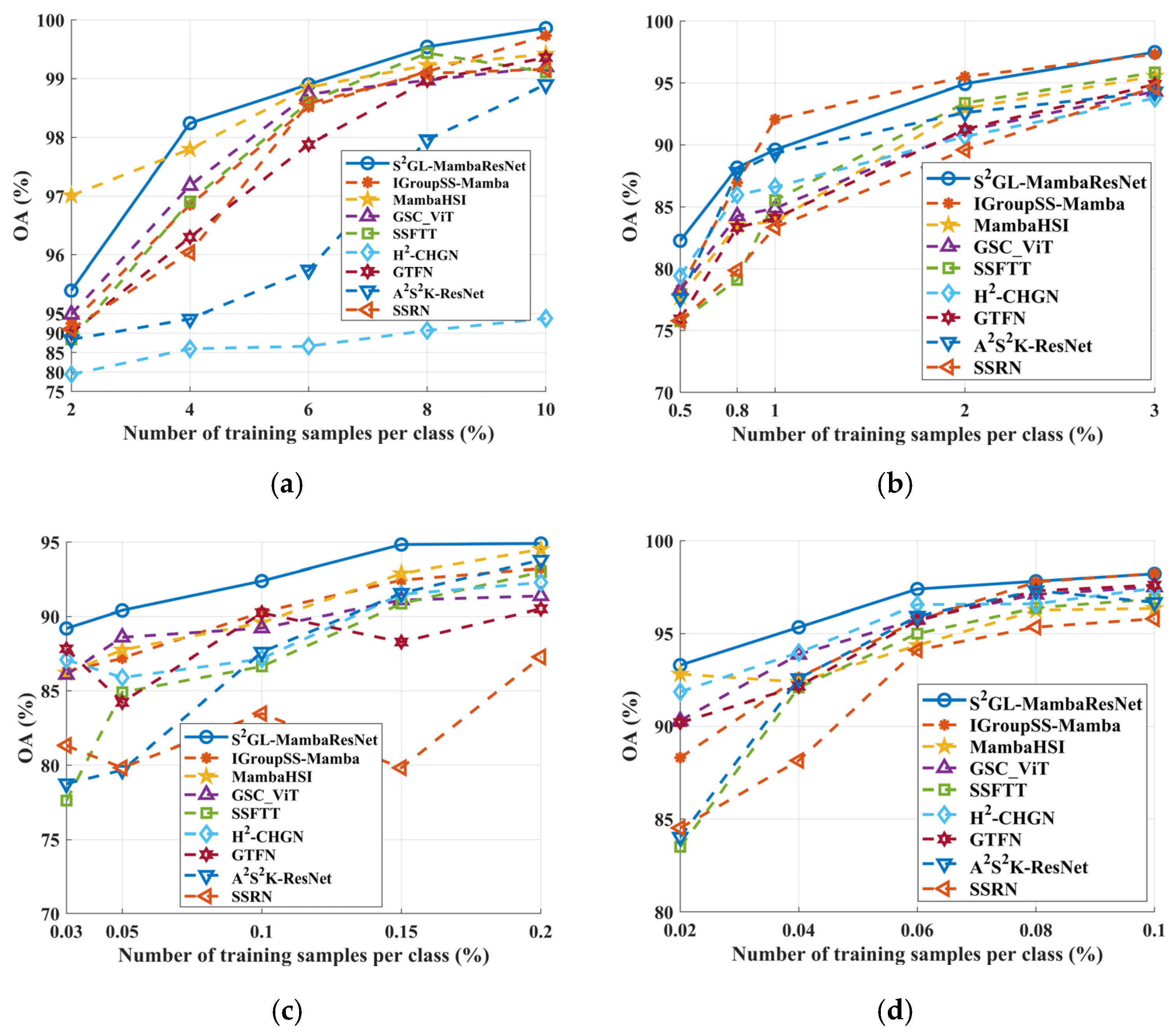
To compare the dependence of S2GL-MambaResNet and competing methods on the number of training samples, we evaluated their classification performance under different training sample ratios. Several representative methods with strong performance were selected for comparison. Figure 12 illustrates the impact of varying the number of training samples on overall accuracy (OA). As shown, the OA of all methods increases as the number of training samples grows.
Figure 12. Influence of the training sample number of each dataset on OA. (a) Botswana. (b) Houston2013 (c) Salinas. (d) WHU-Hi-LongKou. The OA values shown are computed as the mean across 10 independent runs.
On the Botswana dataset, the OA of S2GL-MambaResNet at a 2% training ratio is slightly lower than that of MambaHSI. This may be because, at this ratio, certain land-cover classes contain no training samples, preventing the network from sufficiently learning their characteristics.
On the Houston2013 dataset, S2GL-MambaResNet consistently achieves the best classification performance under both limited and abundant training samples, with OA slightly lower than IGroupSS-Mamba only at the 1% and 2% training ratios. For the Salinas and WHU-Hi-LongKou datasets, S2GL-MambaResNet outperforms all other methods across all training ratios. In contrast, methods such as SSRN and GSC_ViT sometimes exhibit decreased OA as the number of training samples increases, likely due to their limited ability to generalize under data-scarce conditions.
Overall, these results demonstrate that S2GL-MambaResNet can extract high-quality spectral–spatial features and effectively leverage the original image information. It achieves accurate land-cover classification even under few-shot and class-imbalanced scenarios, confirming its robustness.

4. Discussion

4.1. Learned Feature Visualizations by T-SNE

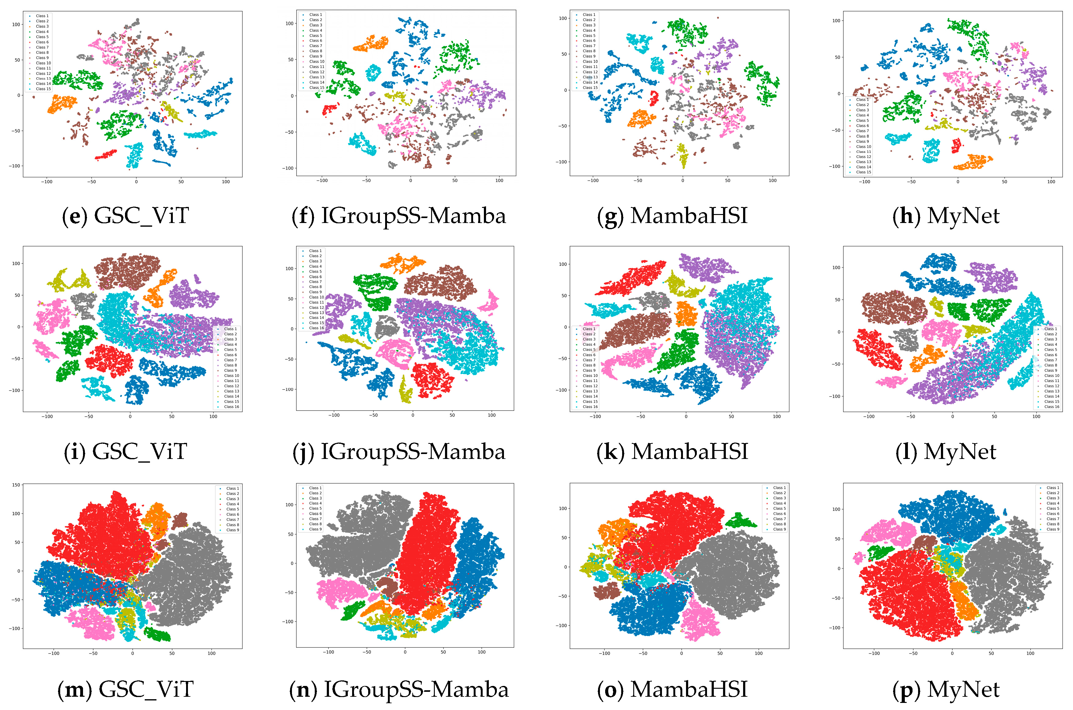
T-distributed stochastic neighbor embedding (t-SNE) [43] is a nonlinear dimensionality reduction technique, particularly suitable for visualizing high-dimensional data. Figure 13 presents the t-SNE results of S2GL-MambaResNet (MyNet) on the four datasets. For clearer visualization, a single spectral band of the features was randomly selected for plotting. It can be observed that samples from the same class cluster together, while samples from different classes are easily separable. Therefore, S2GL-MambaResNet can effectively learn abstract spectral–spatial feature representations. To enable a clearer comparison with existing Mamba methods, we focus on analyzing the t-SNE results of two well-performing networks, MambaHSI and IGroupSS-Mamba. For MambaHSI, the method emphasizes long-range spectral sequence modeling via deep SSMs. Such global modeling often yields tight intra-class compactness for classes that are spectrally distinctive; however, if explicit neighborhood protection is absent prior to serialization, local texture and edge cues can be blurred. In t-SNE projections this effect appears as overlaps between classes that are spatially distinct but spectrally similar—for example, in the WHU-Hi-LongKou dataset class 4 (red) and class 5 (brown) show clear overlap. For IGroupSS-Mamba, the approach reduces redundancy and improves efficiency by group-level and hierarchical summarization. Its embeddings separate classes that differ in coarse spectral morphology well, but to some extent suppress short-range spectral variability and spatial heterogeneity within groups. In t-SNE visualizations this manifests as low overlap and compact clustering for spectrally similar classes—for instance, classes 4 (red) and 5 (brown) do not visibly overlap in WHU-Hi-LongKou—whereas for classes with large spectral differences the inter-class boundaries can appear relatively blurred, reflecting a trade-off between capturing macro-scale spectral differences and preserving fine local features.
Figure 13. t-SNE results of S2GL-MambaResNet on four datasets: (ad) Botswana. (eh) Houston2013. (il) Salinas. (mp) WHU-Hi-LongKou.

4.2. Discussion of Computational Complexity

Since the Botswana dataset has moderate spectral dimensionality and spatial size, we report and compare the trainable parameters (MB), memory (MB), training time (s), inference time (s) and FLOPs (G) of all methods on this dataset, summarized in Table 11. Several observations can be drawn from Table 11. Firstly, although S2GL-MambaResNet (MyNet) has 0.93 MB of trainable parameters—slightly higher than some lightweight methods (e.g., S2Mamba: 0.11 MB, IGroupSS-Mamba: 0.14 MB)—it achieves a highly competitive and practical balance across all resource metrics. It successfully avoids the extreme memory consumption of models like H2-CHGN (7777.88 MB) and MambaHSI (6535.36 MB), as well as the substantial computational overhead of GSC_ViT (518.81 s training time and 21.39 s inference latency). This demonstrates that S2GL-MambaResNet is designed for practical lightweight efficiency, optimizing the overall resource profile rather than a single metric. It is worth noting that S2Mamba significantly enhances the complementarity of spatial-spectral features through linear scanning in four spatial directions and bidirectional scanning in the spectral dimension, achieving efficient computation with minimal parameter cost. However, the highly compact representation space and limited degree of parameterization in this model restrict its ability to learn complex discriminative functions from limited samples. Under imbalanced data distributions, this compactness further amplifies the model’s tendency to overfit dominant categories, making it difficult to capture subtle yet critical spectral differences in long-tailed classes, ultimately leading to reduced recognition rates for minority categories. Secondly, compared with Transformer-based networks, S2GL-MambaResNet avoids extreme resource consumption or long runtime; for example, GSC_ViT requires 518.81 s for training and 52.00 s for inference, while some SSM- and GCN-based networks show very high memory peaks (e.g., H2-CHGN: 7777.88 MB, MambaHSI: 6535.36 MB). Since the Botswana dataset has moderate spectral dimensionality and spatial size, we report and compare the trainable parameters (MB), memory (MB), training time (s), inference time (s), and FLOPs (G) of all methods on this dataset, as summarized in Table 11. Several points can be observed from Table 11. First, although S2GL-MambaResNet (MyNet) has 0.93 MB of trainable parameters—slightly higher than some lightweight methods (e.g., S2Mamba: 0.11 MB, IGroupSS-Mamba: 0.14 MB, SSFTT: 0.15 MB)—it maintains a moderate memory footprint (41.87 MB) and reasonable runtime (training: 215.31 s, inference: 5.96 s). This indicates that the proposed model effectively balances parameter size and computational efficiency. Secondly, when considering computational complexity in terms of FLOPs, S2GL-MambaResNet records 0.7313 G, which is comparable to GTFN (0.7427 G) and significantly lower than MambaHSI (38.56 G) or H2-CHGN (38.82 G). This demonstrates that, despite having slightly more parameters, our model’s actual floating-point operation cost remains low, confirming its lightweight and efficient design in practice. Thirdly, compared with Transformer-based architectures, S2GL-MambaResNet avoids extreme resource consumption and long runtime; for instance, GSC_ViT requires 518.81 s for training and 52.00 s for inference, while certain SSM- and GCN-based networks exhibit very high memory peaks (e.g., H2-CHGN: 7777.88 MB, MambaHSI: 6535.36 MB). In summary, S2GL-MambaResNet achieves a favorable balance between computational complexity and efficiency.
Table 11. Trainable parameters, memory usage, training time, and inference time of all methods on Botswana.

4.3. Outlook and Future Work

There remain areas for improvement in S2GL-MambaResNet. First, in the Botswana dataset (Table 6), although S2GL-MambaResNet achieves the best overall performance, it does not attain the highest accuracy on every single class. This may be due to the dataset’s relatively low spatial resolution (30 m), and high proportion of mixed pixels, limiting the model’s discriminating capability in complex mixed regions. In future work, we plan to explore strategies that explicitly introduce spatial context into the unmixing process. For example, we could adopt the Superpixel Collaborative Sparse Unmixing with Graph Differential Operator [44], which effectively combines local collaboration among superpixels with graph-based spatial regularization to progressively inject spatial-context information into the unmixing pipeline and thereby improve unmixing performance. Alternatively, the Distributed Parallel Geometric Distance (DPGD) method [45] leverages geometric-distance measurements to accurately identify endmembers and estimate their abundances by accounting for intrinsic similarities within hyperspectral images, thus clarifying the underlying data structure and enhancing unmixing accuracy. Secondly, for the WHU-Hi-LongKou dataset (Table 7), while the OA standard deviation remains low, it is slightly higher than that of S2Mamba. This is because, as an H2 dataset, significant intra-class spatial–spectral details and local heterogeneity exist. With very few training samples, it is challenging to fully capture fine-grained feature differences. Although S2GL-MambaResNet is capable of learning such subtle variations, it may also inadvertently incorporate occasional sample-specific characteristics, leading to fluctuations in OA. To mitigate this issue, future work could explore superpixel- or region-based feature aggregation strategies. For example, superpixel-based and spatially regularized diffusion learning [46] first applies entropy-rate superpixel (ERS) segmentation to partition the image into spatially coherent regions and then selects the most representative high-density pixels from each superpixel to construct a spatially regularized diffusion graph [47,48,49,50,51,52,53,54,55,56]. Based on this, superpixel-level regional descriptors or region-level graph structures can be generated, thereby aggregating pixel information within each region to suppress pixel-level noise and sample-specific artifacts. In addition, other methods have also been proposed in recent years [57,58,59,60,61,62,63,64,65].

5. Conclusions

To overcome the loss of spatial coherence and insufficient local spectral perception caused by directly serializing hyperspectral images (HSI) in traditional Mamba networks, this work proposes S2GL-MambaResNet, a lightweight hyperspectral image classification network that tightly couples Mamba with progressive residual fusion. The network is systematically designed through four key strategies: pre-processing before serialization, parallel global and local spatial–spectral modeling, hierarchical group-level spectral modeling, and lightweight progressive residual fusion.
Comparative experiments on four public datasets (Botswana, Houston2013, Salinas, and WHU-Hi-LongKou) demonstrate that S2GL-MambaResNet consistently outperforms other advanced networks in OA, AA, and Kappa under few-shot and class-imbalanced conditions. Specifically, the OA of S2GL-MambaResNet improves on average by 4.36%, 7.99%, 8.53%, and 3.9% on Botswana, Houston2013, Salinas, and WHU-Hi-LongKou, respectively; the AA increases by 5.26%, 8.39%, 11.38%, and 14.18%, and the Kappa rises by 4.71, 8.32, 9.61, and 5.01. Furthermore, the average standard deviations of these three metrics are the lowest among all compared methods, indicating superior generalization capability under limited samples. Qualitative visualizations (Figure 5, Figure 6, Figure 7 and Figure 8) further confirm the advantages of the proposed method in preserving boundary continuity, suppressing noise, and recognizing small objects.
Therefore, S2GL-MambaResNet establishes an effective balance between model complexity and classification performance, offering a practical solution for HSI classification under constrained computational resources and limited training samples.

Author Contributions

Conceptualization, T.C. and H.Y.; methodology, T.C., H.C. and H.Y.; software, G.L.; validation, G.L., Y.P. and J.D.; formal analysis, J.D. and X.Z.; investigation, Y.P.; resources, H.C. and T.C.; data curation, W.D.; writing—original draft preparation, T.C., H.Y., G.L., Y.P., J.D., X.Z. and W.D.; writing—review and editing, H.C. and W.D.; visualization, G.L.; supervision, Y.P.; project administration, H.C.; funding acquisition, H.C. and X.Z. All authors have read and agreed to the published version of the manuscript.

Funding

This work was supported in part by the National Key Research & Development Program of China under Grant 2024YFD1700904; in part by the National Natural Science Foundation of China under Grant 62176217; in part by the Sichuan Science and Technology Program of China under Grant 2023YFS0431; and in part by the China West Normal University Doctoral Startup Project under Grant 22kE018 and the State Key Laboratory of Rail Transit Vehicle System of Southwest Jiaotong University under Grant RVL2511 and 2025RVL-T16.

Data Availability Statement

The raw data supporting the conclusions of this article will be made available by the authors on request.

Conflicts of Interest

Author Guojie Li was employed by the company Dalian Hengyi Technology Co., Ltd. The remaining authors declare that the research was conducted in the absence of any commercial or financial relationships that could be construed as a potential conflict of interest.

References

  1. Long, H.; Chen, T.; Chen, H.; Zhou, X.; Deng, W. Principal space approximation ensemble discriminative marginalized least-squares regression for hyperspectral image classification. Eng. Appl. Artif. Intell. 2024, 133, 108031. [Google Scholar] [CrossRef]
  2. Horita, H. Optimizing runtime business processes with fair workload distribution. J. Compr. Bus. Adm. Res. 2025, 2, 162–173. [Google Scholar] [CrossRef]
  3. Guo, D.; Zhang, S.; Zhang, J.; Yang, B.; Lin, Y. Exploring contextual knowledge-enhanced speech recognition in air traffic control communication: A comparative study. IEEE Trans. Neural Netw. Learn. Syst. 2025, 36, 16085–16099. [Google Scholar] [CrossRef]
  4. Li, M.; Chen, Y.; Lu, Z.; Ding, F.; Hu, B. ADED: Method and device for automatically detecting early depression using multimodal physiological signals evoked and perceived via various emotional scenes in virtual reality. IEEE Trans. Instrum. Meas. 2025, 74, 2524016. [Google Scholar] [CrossRef]
  5. Song, Y.; Song, C. Adaptive evolutionary multitask optimization based on anomaly detection transfer of multiple similar sources. Expert Syst. Appl. 2025, 283, 127599. [Google Scholar] [CrossRef]
  6. Chen, T.; Chen, S.; Chen, L.; Chen, H.; Zheng, B.; Deng, W. Joint classification of hyperspectral and LiDAR data via multiprobability decision fusion method. Remote Sens. 2024, 16, 4317. [Google Scholar] [CrossRef]
  7. Li, Y.; Zhang, H.; Shen, Q. Spectral–spatial classification of hyperspectral imagery with 3D convolutional neural network. Remote Sens. 2017, 9, 67. [Google Scholar] [CrossRef]
  8. Lopatin, A. Intelligent system of estimation of total factor productivity (TFP) and investment efficiency in the economy with external technology gaps. J. Compr. Bus. Adm. Res. 2023, 1, 160–170. [Google Scholar] [CrossRef]
  9. Yang, X.; Ye, Y.; Li, X.; Lau, R.Y.K.; Zhang, X.; Huang, X. Hyperspectral image classification with deep learning models. IEEE Trans. Geosci. Remote Sens. 2018, 56, 5408–5423. [Google Scholar] [CrossRef]
  10. Chhapariya, K.; Buddhiraju, K.M.; Kumar, A. A Deep Spectral–Spatial Residual Attention Network for Hyperspectral Image Classification. IEEE J. Sel. Top. Appl. Earth Observ. Remote Sens. 2024, 17, 15393–15406. [Google Scholar] [CrossRef]
  11. Zhang, S.; Yin, W.; Xue, J.; Fu, Y.; Jia, S. Global–Local Residual Fusion Network for Hyperspectral Image Classification. IEEE Trans. Geosci. Remote Sens. 2025, 63, 5522217. [Google Scholar] [CrossRef]
  12. Xu, R.; Dong, X.-M.; Li, W.; Peng, J.; Sun, W.; Xu, Y. DBCTNet: Double branch convolution-transformer network for hyperspectral image classification. IEEE Trans. Geosci. Remote Sens. 2024, 62, 5509915. [Google Scholar] [CrossRef]
  13. Yu, C.; Zhu, Y.; Wang, Y.; Zhao, E.; Zhang, Q.; Lu, X. Concern With Center-Pixel Labeling: Center-Specific Perception Transformer Network for Hyperspectral Image Classification. IEEE Trans. Geosci. Remote Sens. 2025, 63, 5514614. [Google Scholar] [CrossRef]
  14. Wu, X.; Arshad, T.; Peng, B. Spectral Spatial Window Attention Transformer for Hyperspectral Image Classification. IEEE Trans. Geosci. Remote Sens. 2025, 63, 5519413. [Google Scholar] [CrossRef]
  15. Huang, C.; Song, Y.; Ma, H.; Zhou, X.; Deng, W. A multiple level competitive swarm optimizer based on dual evaluation criteria and global optimization for large-scale optimization problem. Inf. Sci. 2025, 708, 122068. [Google Scholar] [CrossRef]
  16. Chen, Y.; Xu, H.; Liu, J.; Hou, M.; Li, Y.; Qiu, S.; Sun, M.; Zhao, H.; Deng, W. A hybridizing-enhanced quantum-inspired differential evolution algorithm with multi-strategy for complicated optimization. J. Artif. Intell. Soft Comput. Res. 2025, 16, 5–37. [Google Scholar] [CrossRef]
  17. Guo, D.; Zhang, J.; Yang, B.; Lin, Y. Multi-modal intelligent situation awareness in real-time air traffic control: Control intent understanding and flight trajectory prediction. Chin. J. Aeronaut. 2025, 38, 103376. [Google Scholar] [CrossRef]
  18. Deng, W.; Shang, S.; Zhang, L.; Lin, Y.; Huang, C.; Zhao, H.; Ran, X.; Zhou, X.; Chen, H. Multi-strategy quantum differential evolution algorithm with cooperative co-evolution and hybrid search for capacitated vehicle routing. IEEE Trans. Intell. Transp. Syst. 2025, 26, 18460–18470. [Google Scholar] [CrossRef]
  19. Zhao, H.; Chen, Y.; Wang, X.; Wang, D.; Xu, H.; Deng, W. Joint optimization scheduling using AHMQDE-ACO for key resources in smart operations. IEEE Trans. Consum. Electron. 2025. [Google Scholar] [CrossRef]
  20. Gu, A.; Dao, T. Mamba: Linear-time sequence modeling with selective state spaces. arXiv 2023, arXiv:2312.00752. [Google Scholar] [CrossRef]
  21. Dao, T.; Gu, A. Transformers are SSMS: Generalized models and efficient algorithms through structured state space duality. arXiv 2024, arXiv:2405.21060. [Google Scholar] [CrossRef]
  22. Yang, J.X.; Zhou, J.; Wang, J.; Tian, H.; Liew, A.W.C. Hsimamba: Hyperpsectral imaging efficient feature learning with bidirectional state space for classification. arXiv 2024, arXiv:2404.00272. [Google Scholar] [CrossRef]
  23. He, Y.; Tu, B.; Liu, B.; Li, J.; Plaza, A. 3DSS-Mamba: 3D-Spectral-Spatial Mamba for Hyperspectral Image Classification. IEEE Trans. Geosci. Remote Sens. 2024, 62, 5534216. [Google Scholar] [CrossRef]
  24. He, Y.; Tu, B.; Jiang, P.; Liu, B.; Li, J.; Plaza, A. IGroupSS-Mamba: Interval Group Spatial–Spectral Mamba for Hyperspectral Image Classification. IEEE Trans. Geosci. Remote Sens. 2024, 62, 5538817. [Google Scholar] [CrossRef]
  25. Tang, X.; Zhang, Y.; Li, J.; Plaza, A.; Benediktsson, J.A. SpiralMamba: Spatial–Spectral Complementary Mamba With Spatial Spiral Scan for Hyperspectral Image Classification. IEEE Trans. Geosci. Remote Sens. 2025, 63, 5510319. [Google Scholar] [CrossRef]
  26. Zhao, H.; Liu, C.; Dang, X.; Xu, J.; Deng, W. Few-shot cross-domain fault diagnosis of transportation motor bearings using MAML-GA. IEEE Trans. Transp. Electrif. 2025. [Google Scholar] [CrossRef]
  27. Ali, A.; Agrawal, S.; Dongre, S. Blockchain-based NFT warranty system: A software implementation. J. Compr. Bus. Adm. Res. 2024, 1, 12–18. [Google Scholar] [CrossRef]
  28. Deng, W.; Xu, H.; Guan, Z.; Sun, Y.; Ran, X.; Ma, H.; Zhou, X.; Zhao, H. PSO-K-means clustering-based NSGA-III for delay recovery. IEEE Trans. Consum. Electron. 2025. [Google Scholar] [CrossRef]
  29. Zhao, H.; Gu, M.; Qiu, S.; Zhao, A.; Deng, W. Dynamic path planning for space-time optimization cooperative tasks of multiple unmanned aerial vehicles in uncertain environment. IEEE Trans. Consum. Electron. 2025, 71, 7673–7682. [Google Scholar] [CrossRef]
  30. Li, X.; Zhao, H.; Xu, J.; Zhu, G.; Deng, W. APDPFL: Anti-poisoning attack decentralized privacy enhanced federated learning scheme for flight operation data sharing. IEEE Trans. Wirel. Commun. 2024, 23, 19098–19109. [Google Scholar] [CrossRef]
  31. Deng, W.; Li, X.; Xu, J.; Li, W.; Zhu, G.; Zhao, H. BFKD: Blockchain-based federated knowledge distillation for aviation internet of things. IEEE Trans. Reliab. 2025, 7, 2626–2639. [Google Scholar] [CrossRef]
  32. Yao, R.; Zhao, H.; Zhao, Z.; Guo, C.; Deng, W. Parallel convolutional transfer network for bearing fault diagnosis under varying operation states. IEEE Trans. Instrum. Meas. 2024, 73, 3540713. [Google Scholar] [CrossRef]
  33. Li, Y.; Luo, Y.; Zhang, L.; Wang, Z.; Du, B. MambaHSI: Spatial–Spectral Mamba for Hyperspectral Image Classification. IEEE Trans. Geosci. Remote Sens. 2024, 62, 5524216. [Google Scholar] [CrossRef]
  34. Wang, Q.; Wu, B.; Zhu, P.; Li, P.; Zuo, W.; Hu, Q. ECA-Net: Efficient Channel Attention for Deep Convolutional Neural Networks. arXiv 2019, arXiv:1910.03151. [Google Scholar]
  35. Zhong, Y.; Hu, X.; Luo, C.; Wang, X.; Zhao, J.; Zhang, L. WHU-Hi: UAV-borne hyperspectral with high spatial resolution (H2) benchmark datasets and classifier for precise crop identification based on deep convolutional neural network with CRF. Remote Sens. Environ. 2020, 250, 112012. [Google Scholar] [CrossRef]
  36. Zhong, Z.; Li, J.; Luo, Z.; Chapman, M. Spectral–spatial residual network for hyperspectral image classification: A 3-D deep learning framework. IEEE Trans. Geosci. Remote Sens. 2017, 56, 847–858. [Google Scholar] [CrossRef]
  37. Roy, S.K.; Manna, S.; Song, T.; Bruzzone, L. Attention-based adaptive spectral–spatial kernel ResNet for hyperspectral image classification. IEEE Trans. Geosci. Remote Sens. 2020, 59, 7831–7843. [Google Scholar] [CrossRef]
  38. Yang, A.; Li, M.; Ding, Y.; Hong, D.; Lv, Y.; He, Y. GTFN: GCN and transformer fusion network with spatial-spectral features for hyperspectral image classification. IEEE Trans. Geosci. Remote Sens. 2023, 61, 6600115. [Google Scholar] [CrossRef]
  39. Chen, T.; Wang, T.; Chen, H.; Zheng, B.; Deng, W. Cross-Hopping Graph Networks for Hyperspectral–High Spatial Resolution (H2) Image Classification. Remote Sens. 2024, 16, 3155. [Google Scholar] [CrossRef]
  40. Sun, L.; Zhao, G.; Zheng, Y.; Wu, Z. Spectral–spatial feature tokenization transformer for hyperspectral image classification. IEEE Trans. Geosci. Remote Sens. 2022, 60, 5522214. [Google Scholar] [CrossRef]
  41. Zhao, Z.; Xu, X.; Li, S.; Plaza, A. Hyperspectral image classification using groupwise separable convolutional vision transformer network. IEEE Trans. Geosci. Remote Sens. 2024, 62, 5511817. [Google Scholar] [CrossRef]
  42. Wang, G.; Zhang, X.; Peng, Z.; Zhang, T.; Jiao, L. S2Mamba: A Spatial–Spectral State Space Model for Hyperspectral Image Classification. IEEE Trans. Geosci. Remote Sens. 2025, 63, 5511413. [Google Scholar] [CrossRef]
  43. Maaten, L.; Hinton, G. Visualizing data using t-SNE. J. Mach. Learn. Res. 2008, 9, 2579–2605. [Google Scholar]
  44. Yang, K.; Zhao, Z.; Yang, Q.; Feng, R. SCSU–GDO: Superpixel Collaborative Sparse Unmixing with Graph Differential Operator for Hyperspectral Imagery. Remote Sens. 2025, 17, 3088. [Google Scholar] [CrossRef]
  45. Cañada, C.; Paoletti, M.E.; García-Flores, M.B.; Tao, X.; Pastor-Vargas, R.; Haut, J.M. Distributed Parallel Hyperspectral Unmixing for Large-Scale Data in Spark Environments via Geometric Distance. IEEE Trans. Geosci. Remote Sens. 2025, 63, 5531719. [Google Scholar] [CrossRef]
  46. Cui, K.; Li, R.; Polk, S.L.; Lin, Y.; Zhang, H.; Murphy, J.M.; Plemmons, R.J.; Chan, R.H. Superpixel-based and spatially regularized diffusion learning for unsupervised hyperspectral image clustering. IEEE Trans. Geosci. Remote Sens. 2024, 62, 4405818. [Google Scholar] [CrossRef]
  47. Zhang, M.; Yang, Y.; Zhang, S.; Mi, P.; Han, D. CPMFFormer: Class-Aware Progressive Multiscale Fusion Transformer for Hyperspectral Image Classification. Remote Sens. 2025, 17, 3684. [Google Scholar] [CrossRef]
  48. Zhao, A.; Feng, R.; Li, X. ThiefCloud: A Thickness Fused Thin Cloud Removal Network for Optical Remote Sensing Image With Self-Supervised Learnable Cloud Prior. IEEE Trans. Circuits Syst. Video Technol. 2025. [Google Scholar] [CrossRef]
  49. Xu, Y.; Yu, W.; Ghamisi, P.; Kopp, M.; Hochreiter, S. Txt2Img-MHN: Remote sensing image generation from text using modern Hopfield networks. IEEE Trans. Image Process. 2023, 32, 5737–5750. [Google Scholar] [CrossRef]
  50. Huang, C.; Wu, D.; Zhou, X.; Song, Y.; Chen, H.; Deng, W. Competitive swarm optimizer with dynamic multi-competitions and convergence accelerator for large-scale optimization problems. Appl. Soft Comput. 2024, 167, 112252. [Google Scholar] [CrossRef]
  51. Zhao, H.; Zhang, J.; Lin, L.; Wang, J.; Gao, S.; Zhang, Z. Locally linear unbiased randomization network for cross-scene hyperspectral image classification. IEEE Trans. Geosci. Remote Sens. 2023, 61, 5526512. [Google Scholar] [CrossRef]
  52. Bai, X.; Li, X.; Miao, J.; Shen, H. A front-back view fusion strategy and a novel dataset for super tiny object detection in remote sensing imagery. Knowl.-Based Syst. 2025, 326, 114051. [Google Scholar] [CrossRef]
  53. Dong, L.; Geng, J.; Jiang, W. Spectral-Spatial Enhancement and Causal Constraint for Hyperspectral Image Cross-Scene Classification. IEEE Trans. Geosci. Remote Sens. 2024, 62, 5507013. [Google Scholar] [CrossRef]
  54. Wu, Z.; Zhen, H.; Zhang, X.; Bai, X.; Li, X. SEMA-YOLO: Lightweight Small Object Detection in Remote Sensing Image via Shallow-Layer Enhancement and Multi-Scale Adaptation. Remote Sens. 2025, 17, 1917. [Google Scholar] [CrossRef]
  55. Yuan, Z.; Zhang, W.; Tian, C.; Rong, X.; Zhang, Z.; Wang, H.; Fu, K.; Sun, X. Remote sensing cross-modal text-image retrieval based on global and local information. IEEE Trans. Geosci. Remote Sens. 2022, 60, 5620616. [Google Scholar] [CrossRef]
  56. Li, Y.; Zhu, Z.; Yu, J.G.; Zhang, Y. Learning deep cross-modal embedding networks for zero-shot remote sensing image scene classification. IEEE Trans. Geosci. Remote Sens. 2021, 59, 10590–10603. [Google Scholar] [CrossRef]
  57. Roy, S.K.; Jamali, A.; Chanussot, J.; Ghamisi, P.; Ghaderpour, E.; Shahabi, H. SimPoolFormer: A two-stream vision transformer for hyperspectral image classification. Remote Sens. Appl. Soc. Environ. 2025, 37, 101478. [Google Scholar] [CrossRef]
  58. Alkhatib, M.Q.; Al-Saad, M.; Aburaed, N.; Almansoori, S.; Zabalza, J.; Marshall, S.; Al-Ahmad, H. Tri-CNN: A three branch model for hyperspectral image classification. Remote Sens. 2023, 15, 316. [Google Scholar] [CrossRef]
  59. Cao, X.; Yao, J.; Xu, Z.; Meng, D. Hyperspectral image classification with convolutional neural network and active learning. IEEE Trans. Geosci. Remote Sens. 2020, 58, 4604–4616. [Google Scholar] [CrossRef]
  60. Xie, C.; Zhou, L.; Ding, S.; Lu, M.; Zhou, X. Research on self-propulsion simulation of a polar ship in a brash ice channel based on body force model. Int. J. Nav. Archit. Ocean Eng. 2023, 15, 100557. [Google Scholar] [CrossRef]
  61. Deng, W.; Li, K.; Zhao, H. A flight arrival time prediction method based on cluster clustering-based modular with deep neural network. IEEE Trans. Intell. Transp. Syst. 2024, 25, 6238–6247. [Google Scholar] [CrossRef]
  62. Han, S.; Yan, L.; Sun, J.; Ding, S.; Li, F.; Diao, F.; Zhou, L. Hybrid trajectory planning and tracking for automatic berthing: A grid-search and optimal control integration approach. Ocean Eng. 2025, 317, 120002. [Google Scholar] [CrossRef]
  63. Ran, X.; Suyaroj, N.; Tepsan, W.; Lei, M.; Ma, H.; Zhou, X.; Deng, W. A novel fuzzy system-based genetic algorithm for trajectory segment generation in urban global positioning system. J. Adv. Res. 2025; in press. [Google Scholar] [CrossRef]
  64. Han, S.; Sun, J.; Yan, L.; Ding, S.; Zhou, L. Research on effective trajectory planning, tracking, and reconstruction for USV formation in complex environments. Ocean Eng. 2025, 341, 122488. [Google Scholar] [CrossRef]
  65. Ma, Q.J.; Jiang, J.; Liu, X.M.; Ma, J.Y. Learning a 3D-CNN and Transformer Prior for Hyperspectral Image Super-Resolution. Inf. Fusion 2023, 100, 101907. [Google Scholar] [CrossRef]
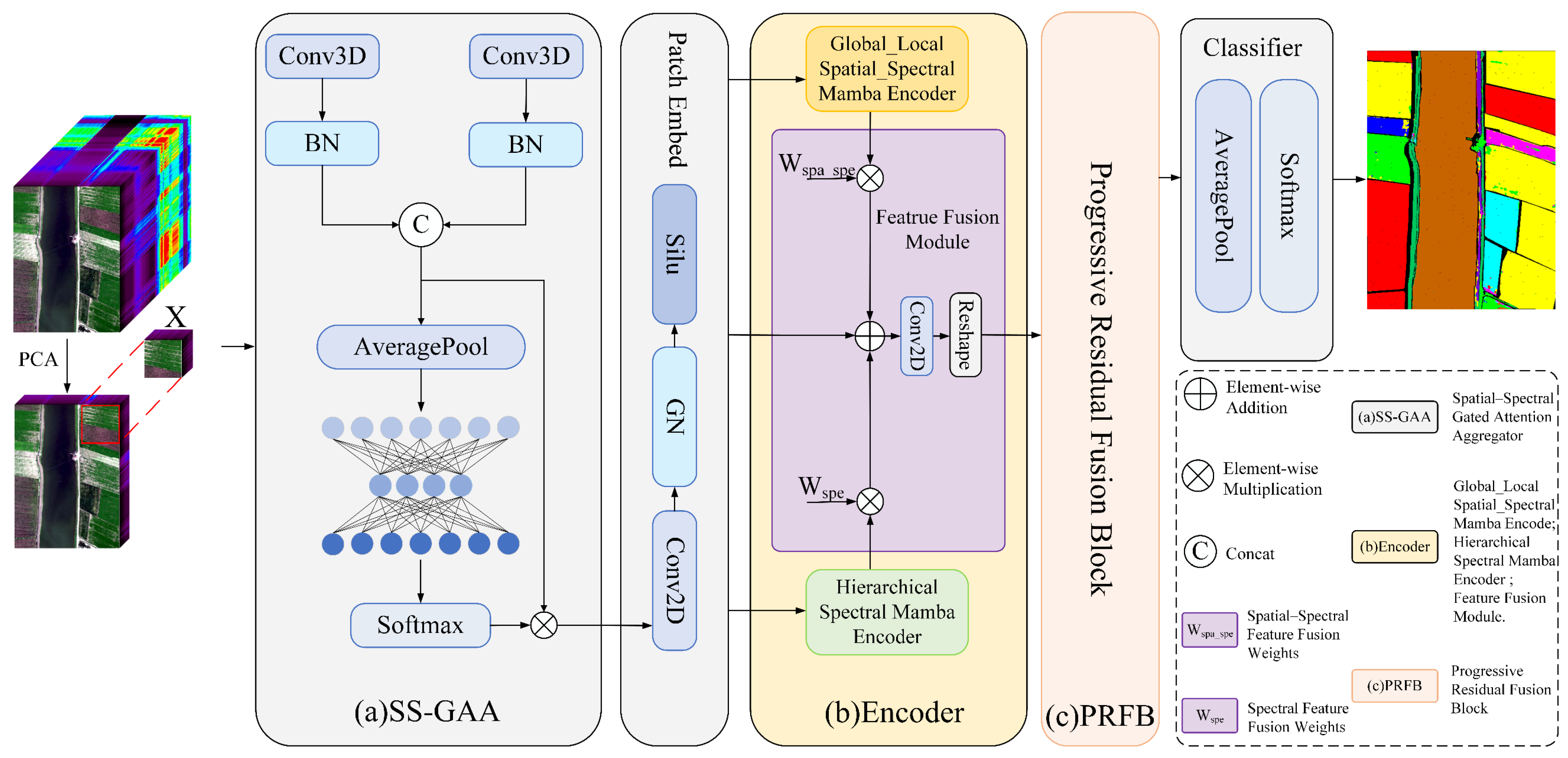
Disclaimer/Publisher’s Note: The statements, opinions and data contained in all publications are solely those of the individual author(s) and contributor(s) and not of MDPI and/or the editor(s). MDPI and/or the editor(s) disclaim responsibility for any injury to people or property resulting from any ideas, methods, instructions or products referred to in the content.

Article Metrics

Citations

Article Access Statistics

Article metric data becomes available approximately 24 hours after publication online.