Graph-Based Relaxation for Over-Normalization Avoidance in Reflectance Normalization of Multi-Temporal Satellite Imagery

Highlights

What are the main findings?

• The proposed graph-based relaxation demonstrates a strong ability to balance reflectance consistency and temporal variability. The method successfully addresses under-normalization and over-normalization, two significant difficulties that commonly distort temporal assessments in multitemporal satellite data through the incorporation of intra-normalization and inter-normalization into a graph-based framework. This balance allows the model to maintain radiometric consistency across different acquisition periods and sensors while preserving the seasonal characteristics of each image, resulting in accurate normalization without significant variance loss.
• The proposed method also demonstrated remarkable capability in preserving seasonal and environmental dynamics, particularly in maintaining NDVI trends that reflect natural vegetation cycles. Compared to standard normalization procedures, which frequently result in over-smoothing or temporal discontinuities, the proposed graph-based relaxation preserved seasonal variability while ensuring smooth transitions between distinct periods. As a result, it generated clearer and more realistic representations of vegetation and environmental changes over time, providing higher confidence for long-term monitoring and ecosystem trend assessments.

What are the implications of the main findings?

• By maintaining both temporal stability and seasonal variability, the proposed method increases confidence in long term environmental monitoring results. It minimizes temporal distortions caused by under-normalization and over-normalization, ensuring that reflectance trends represent environmental and phenological changes over time. The framework also achieves consistent reflectance alignment across Landsat 8, Landsat 9, and Sentinel 2 imagery, enabling smooth cross-sensor harmonization through robust linear radiometric alignment necessary for temporal studies and supporting the integration of multi-sensor satellite archives.
• The graph-based relaxation framework demonstrates strong scalability and automation potential. Its adaptable structure supports integration into machine learning workflows or AI-assisted preprocessing pipelines, specifically by decomposing the time series into parallelizable subgraphs, allowing for efficient handling of large-scale datasets. This makes the method suitable for operational use in long-term, spatiotemporal Earth observation projects that require consistent, season-aware reflectance normalization.

Abstract

Reflectance normalization is critical for minimizing temporal discrepancies and facilitating reliable multi-temporal satellite analysis. However, this process is challenged by the risks of under-normalization and over-normalization, which stem from the inherent complexities of varying atmospheric conditions, data acquisition, and environmental dynamics. Under-normalization occurs when multi-temporal variations are insufficiently corrected, resulting in temporal reflectance inconsistencies. Over-normalization arises when overly aggressive adjustments suppress meaningful variability, such as seasonal and phenological patterns, thereby compromising data integrity. Effectively addressing these challenges is essential for preserving the spatial and temporal fidelity of satellite imagery, which is crucial for applications such as environmental monitoring and long-term change analysis. This study introduces a novel graph-based relaxation for reflectance normalization aimed at addressing issues of under- and over-normalization through a two-stage structural normalization strategy: intra-normalization and inter-normalization. A graph structure represents adjacency and similarity among image instances, enabling an iterative relaxation process to adjust reflectance values. In the proposed framework, the intra-normalization stage aligns images within the same reflectance group to preserve temporally local reflectance patterns, while the inter-normalization stage harmonizes reflectance across different groups, ensuring smooth temporal transitions and maintaining essential temporal variability. Experimental results with the metrics root mean squared error (RMSE) and Structural Similarity Index Measure (SSIM) demonstrate the effectiveness of the proposed method. Specifically, the proposed method achieves around 37% improvement measured by RMSE in the transition of two adjacent image groups compared with related normalization methods. Graph-based relaxation preserves seasonal dynamics, ensures smooth transitions, and improves vegetation indices, making it suitable for both short-term and long-term environmental change analysis.

1. Introduction

Reflectance normalization is an essential process for the analysis of multi-temporal or cross-sensor satellite imagery [1,2]. This process aims to alleviate temporal reflectance inconsistencies while preserving local temporal patterns such as seasonal changes by adjusting the reflectance of satellite images acquired under different sensors, acquisition days, and environmental conditions onto a common reflectance scale [3]. Such harmonization ensures consistent and reliable reflectance data for remote-sensing applications such as land cover classification, vegetation monitoring, and climate change analyses [4,5,6].

Many normalization methods have been developed to address radiometric and reflectance inconsistencies in multi-temporal and even multi-sensor satellite images. They can be classified into two categories: absolute radiometric normalization (ARN) and relative radiometric normalization (RRN) [7,8]. ARN techniques aim to convert optical satellite imagery from raw digital numbers to surface reflectance values [9]. This is typically achieved through physically based atmospheric correction models, particularly radiative transfer models such as the Second Simulation of the Satellite Signal in the Solar Spectrum (6S), the Moderate Resolution Atmospheric Transmission (MODTRAN), and the Fast Line-of-sight Atmospheric Analysis of Spectral Hypercubes (FLAASH) [10,11,12]. These models simulate the interaction between solar radiation and atmospheric components, including aerosols, gases, and water vapor, to correct satellite images [13]. Accurate correction requires auxiliary data such as sun-sensor geometry, surface elevation, and atmospheric profiles. As a result, ARN methods provide radiometrically consistent and physically correct reflectance outputs, making them valuable for long-term environmental monitoring and change detection. However, the effectiveness of ARN is often limited by the availability and accuracy of atmospheric or calibration data, which is rare in remote or under-instrumented areas.

In contrast, RRN methods do not attempt to retrieve physically based surface reflectance values. Instead, they focus on minimizing radiometric inconsistencies by aligning target images with a reference image [14,15]. RRN techniques are valued for their simplicity, cost-effectiveness, and flexibility, especially in short-term normalization tasks where atmospheric and seasonal variations are relatively minor. The RRN approaches generally involve the use of pseudo-invariant features (PIFs), which are the features such as roads, buildings, and bare soil that exhibit relatively stable reflectance over time regardless of atmospheric or illumination conditions [16,17]. The PIFs are identified from multi-temporal images, and then statistical methods such as linear regression or transformation functions are applied to adjust the radiometric/reflectance values of the target images to that of the reference image [18,19]. Other common RRN methods include dark object subtraction (DOS), which assumes that certain dark surfaces have near-zero reflectance [20,21], and histogram matching, which aligns the brightness distribution of a target image to match that of the reference image. However, the effectiveness of these methods depends on the selection of a high-quality reference image and the accurate identification of PIFs. Errors in either step can introduce biases or artifacts in the normalized output.

One of the earlier efforts employing deep learning for radiometric correction used a CycleGAN-based approach for relative radiometric adjustment in high-resolution remote-sensing images [22]. It followed a deep learning architecture that jointly performs radiometric harmonization and super-resolution [23]. Their method reconciles spectral and temporal inconsistencies between the two sensors while also enhancing spatial resolution. Then, radiometric normalization was performed through latent change noise learning [24]. Instead of relying on PIFs, their probabilistic framework learns to disentangle radiometric distortions from true surface changes, providing improved robustness in settings where traditional RRN methods fail due to significant scene variations.

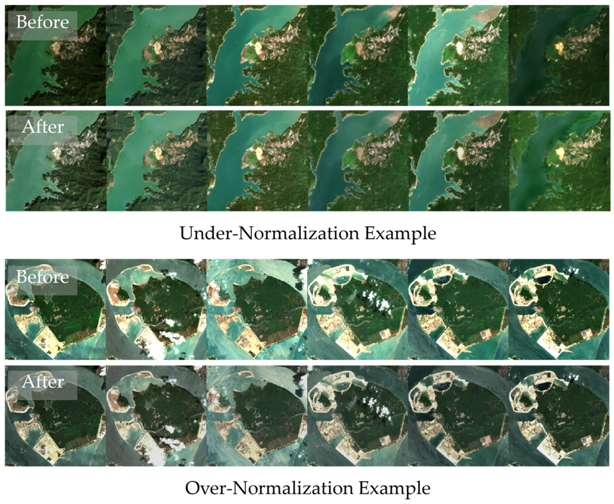
While absolute radiometric normalization (ARN), relative radiometric normalization (RRN), and any advance methods are effective at reducing radiometric inconsistencies, they typically depend on grouping images into seasonally clusters to manage non-linear temporal variations. However, these designs introduce two major limitations. First, images near the boundaries of a seasonal group may be insufficiently adjusted, resulting in under-normalization. Second, if the chosen reference image does not adequately represent the full variability of the season, normalization may become overly constrained, leading to over-normalization and suppression of meaningful reflectance differences within the cluster. These issues are illustrated in Figure 1. These two issues may reduce the reliability and usability of multi-temporal satellite images. Under-normalization occurs when the normalization process does not sufficiently correct radiometric discrepancies between images [25]. Quantitatively, under-normalization is characterized by high root mean square error (RMSE) or mean absolute error (MAE), and a low SSIM value indicates that reflectance inconsistencies remain. These inconsistencies may obscure temporal radiometric trends, which will degrade the performance of downstream applications such as phenological monitoring and anomaly detection. In contrast, over-normalization arises when the normalization process enforces excessive uniformity across images, thereby suppressing genuine temporal variability. It is characterized by low RMSE or MAE and overly high SSIM between the images because the images have been homogenized. This issue is generally caused by overfitting to radiometric or reflectance similarity. As a result, over-normalization may eliminate temporal signals such as seasonal dynamics, ecological changes, and time-series classification, which are essential for many remote-sensing analyses [26].

Figure 1. Examples of under-normalization (top) and over-normalization (bottom). The first row displays the images before normalization, and the second row shows the corresponding images after normalization.

To address the under- and over-normalization of satellite images, this study proposes graph-based relaxation, a balanced normalization framework that maintains local reflectance variability while preserving overall consistency. The proposed graph-based relaxation framework operates within the RRN domain, utilizing established RRN components (IR-MAD and regression) not to replace them, but to structurally enhance RRN’s capability to manage the chronic temporal stability. The framework consists of two stages: intra-normalization and inter-normalization. The intra-normalization stage adjusts images within an image group to preserve local temporal consistency. In contrast, the inter-normalization stage ensures smooth transitions between adjacent image groups. By integrating these two stages with a relaxation-based normalization, the framework achieves a balance between global reflectance consistency and the preservation of fine-scale temporal dynamics. This makes the method well-suited for long-term, multi-temporal, and cross-sensor image analyses.

2. Materials and Methods

2.1. System Overview

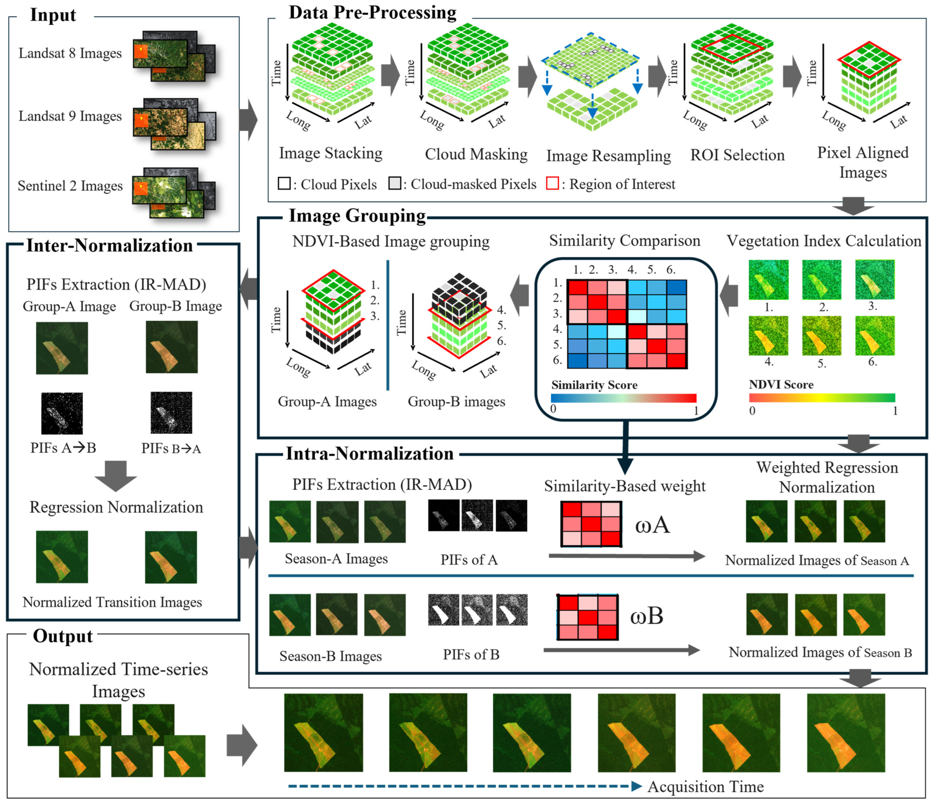
A graph-based relaxation for reflectance normalization is proposed to address under- and over-normalization in cross-sensor and multi-temporal satellite images. Figure 2 illustrates the workflow of the method, which consists of three main steps: data pre-processing, image grouping, and reflectance normalization. The input is a set of surface reflectance images from three optical satellite sensors: Landsat 8, Landsat 9, and Sentinel-2. Six commonly used multispectral bands, including three visible bands (red, green, blue) and three infrared bands (Near-Infrared, SWIR1, and SWIR2), are selected for cross-sensor normalization and vegetation index analyses. In the data pre-processing, all images are stacked by chronological order, and images are resampled to a uniform spatial resolution. Next, image grouping is performed based on image similarity. The normalized difference vegetation index (NDVI) is computed for each image to capture rough vegetation dynamics, and the structural similarity index measure (SSIM) is used to evaluate visual and textural similarity between NDVI images. Based on the SSIM scores, images are semi-automatically grouped into distinct groups. The third step is graph-based reflectance normalization, in which the relaxation normalization contains two stages: inter-normalization and intra-normalization. The stage of inter-normalization focuses on the normalization of transition images to ensure smooth radiometric continuity between adjacent image groups. These normalized transition images are then used as anchors in the stage of intra-normalization, which aligns the remaining images within each group by using relaxation. The integrity of these anchors is important for this structure. If a normalized transition anchor is biased, that error can be propagated to all other images in the seasonal group, leading to over-normalization or under-normalization across the entire cluster. SSIM values are used as weights in the graph-based relaxation process, enabling the normalization to reflect each image’s relative similarity within its group. This two-stage process ensures both reflectance consistency and seasonal fidelity across the time series. In this section, the graph design and image grouping are described in Section 2.2; the proposed graph-based relaxation for reflectance normalization is presented in Section 2.3.

Figure 2. Workflow of the proposed graph-based relaxation for reflectance normalization. Images (1)–(6) illustrate the selected and pre-processed cross-sensor images used in the framework, with different colors representing distinct multi-temporal acquisition dates.

2.2. Graph Design and Image Grouping

There are three graph structures, shown in Figure 3, employed in relaxation-based normalization. In graph theory, a graph $G=\left(V,E\right)$ is a structure consisting of a set of vertices V and a set of edges E that connect pairs of vertices [27]. In the context of this study, a vertex corresponds to an image in a dataset while an edge represents a normalization relationship between two images. The graph structure determines how the image reflectance is adjusted and propagated across the image series in a dataset.

Figure 3. Illustration of the radiometry normalization graphs for images from three sensors (Sensors X, Y, and Z). Left: ring graph. Middle: fully connected graph. Right: season-aware graph. ‘t’ represents image acquisition time.

The first structure is a ring graph denoted as $G_{RG}=\left(V,E_{Ring}\right)$, where $V=\left\{I_1,\cdots ,I_n\right\}$ represents a set of n cross-sensor images sorted by acquisition day, and $E_{Ring}={\left\{\left(I_i,I_{\left(i+1\right)modn}\right)\right\}}_{i=1}^n$ represents the set of connections between two temporally immediate image neighbors. The graph $G_{RG}$ connects each image $I_i\in V$ only to its immediate temporal neighbors $I_{i-1}$ and $I_{i+1}$, forming a closed sequential loop. This structure performs pairwise normalization between adjacent images in chronological order, and the simplicity and low computational cost make the graph $G_{RG}$ suitable for scenarios that require efficient processing while maintaining local consistency. The second structure is a fully connected graph denoted as $G_{FG}=\left(V,E_{full}\right)$, where $E_{full}=\left\{\left(I_i,I_j\right)|i\ne j,1\le i,j\le n\right\}$. This structure connects every image to all other images in a dataset, which allows for normalization across all image pairs to maximize information sharing. Hence, the graph $G_{FG}$ can promote global reflectance consistency and normalization stability. The conventional structures, $G_{RG}$ and $G_{FG}$, represent two cluster configurations. $G_{RG}$ models a simple sequential correction, often resulting in boundary discontinuities (under-normalization) when crossing seasonal cluster. $G_{FG}$ models an overly dense cluster connection, which enforces global consistency at the cost of suppressing vital temporal variability (over-normalization). The third graph is a proposed season-aware graph represented as $G_{SG}={\left\{G_{intra}^i:\left(V_{intra}^i,E_{intra}^i\right),:G_{inter}:\left(V_{inter},E_{inter}\right)\right\}}_{i=1}^{i=q}$, which contains q similarity subgraphs ${\left\{G_{intra}^i:\left(V_{intra}^i,E_{intra}^i\right)\right\}}_{i=1}^{i=q}$ and one inter-normalization subgraph $G_{inter}:\left(V_{inter},E_{inter}\right)$. The graph $G_{SG}$ is designed as an adaptive, two-stage architecture that explicitly manages the trade-off inherent in seasonal clustering. It achieves this by structurally separating intra-cluster from inter-cluster transition smoothing.

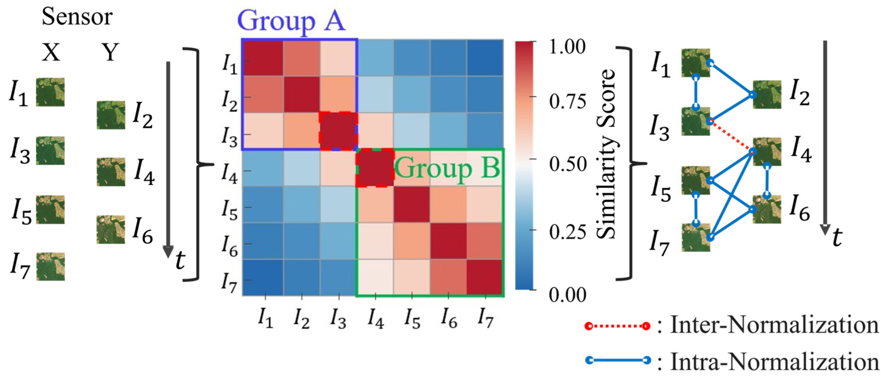
In Figure 4, for instance, the dataset is divided into two similarity groups, A and B, and one transition group containing $I_3$ and $I_4.$ The identification of this transition group is crucial because it allows the normalization process to preserve local seasonal variability while preventing error accumulation at the boundaries between cluster. Then, the grouping step organizes images according to their seasonal similarity so that contextually related images are normalized together. This structure allows the graph to represent both local seasonal relationships and season-to-season transitions. Image similarity for this grouping is measured by SSIM, which is defined as

$$SSIM({\widehat{I}}_X,{\widehat{I}}_Y)={\displaystyle \frac{(2{\mu }_{{\widehat{I}}_X}{\mu }_{{\widehat{I}}_Y}+C_1)(2{\sigma }_{{\widehat{I}}_X{\widehat{I}}_Y}+C_2)}{({\mu }_{{\widehat{I}}_X}^2+{\mu }_{{\widehat{I}}_Y}^2+C_1)({\sigma }_{{\widehat{I}}_X}^2+{\sigma }_{{\widehat{I}}_Y}^2+C_2)}},$$

(1)

where ${\widehat{I}}_X$ and ${\widehat{I}}_Y$ present the NDVIs of the images $I_X$ and $I_Y$, ${\mu }_{{\widehat{I}}_X}$ and ${\sigma }_{{\widehat{I}}_X}^2$ denote the mean and variance of the NDVI image ${\widehat{I}}_X$, respectively, ${\sigma }_{{\widehat{I}}_X{\widehat{I}}_Y}$ represents the covariance of ${\widehat{I}}_X$ and ${\widehat{I}}_Y$, and $C_1$ and $C_2$ are small constants to stabilize the division when denominators are close to zero. Images with higher SSIM values exhibit more similar NDVI patterns, and images with similar NDVI patterns are likely to be clustered into a group. In Figure 4, for instance, the dataset is divided into two similarity groups, that is, groups A and B, and one transition group containing images $I_3$ and $I_4.$ This clustering preserves local variability while reducing the possibility of over-normalization.

Figure 4. Example of similarity-based image grouping. Left: Input image sequence. Middle: Image grouping based on the similarity matrix, showing Season Group A Season Group B and transition images $I_3$ and $I_4$. Right: $G_{FC}$-based season-aware graph $G_{SG}$.

After the image grouping, two kinds of subgraphs for structural decomposition are constructed, intra-subgraph $G_{intra}^j:{\left\{\left(V_{intra}^j,E_{intra}^j\right)\right\}}_{j=1}^{j=q}$ and inter-subgraph $G_{inter}:\left(V_{inter},E_{inter}\right)$ which manages the time-series as clusters connected by boundary smoothing. An intra-subgraph represents a similar image group, and a ring subgraph $G_{RG}$ or a fully connected subgraph $G_{FG}$ can be assigned to be the intra-subgraph. The inter-subgraph $G_{inter}$ contains the transition images $V_{inter}$ and the edges $E_{inter}$ connecting different seasonal groups. This design enables a two-stage normalization process. In the first stage, inter-normalization adjusts the transition images $\left\{I_{inter,1},\cdots ,V_{inter,k}\right\}$ in the set $V_{inter}$, where $k$ represents the number of transition images, to harmonize reflectance between seasonal groups. In the second stage, intra-normalization aligns images $V_{intra}^j=\left\{I_{intra,1}^i,\cdots ,I_{intra,l}^i\right\}$, where $l$ denotes the number of seasonal images in the intra-subgraph $G_{intra}^j$ by using relaxation-based reflectance normalization with the normalized transition images obtained in the first stage as anchors. With these two stages, balanced normalization can be achieved, which maintains global reflectance consistency while preserving temporal variability.

2.3. Image Normalization

Image normalization is a process to improve the consistency of surface reflectance of multi-temporal and multi-sensor images [28,29]. The normalization process aims to reduce the reflectance discrepancies stemming from different atmospheric conditions, sensors, and seasonal changes while preserving essential information above the surface of the Earth [28,30]. The normalization in this study is a relaxation-based normalization that adopts the Iteratively Reweighted Multivariate Alteration Detection (IR-MAD) method for PIF selection and regression-based reflectance adjustment. IR-MAD, based on conventional MAD, is an automatic process widely used for the selection of PIFs between image pairs [31,32]. IR-MAD begins with the computation of MAD variates between a target image $I_T$ and a reference image $I_R$ with $m$ spectral bands. Through the canonical correlation analysis, the eigenvectors $\mathsf{\alpha }=\left({\alpha }_1,\cdots ,{\alpha }_m\right)$ and $\mathsf{\beta }=\left({\beta }_1,\cdots ,{\beta }_m\right)$ and their corresponding eigenvalues are obtained. The MAD variates ranking from highest to lowest are calculated using

$$\left[\begin{array}{c}{MAD}_1\\ \begin{array}{c}{MAD}_2\\ ⋮\end{array}\\ {MAD}_m\end{array}\right]=\left[\begin{array}{c}{\alpha }_m{I}_T-{\beta }_m{I}_R\\ \begin{array}{c}\begin{array}{c}{\alpha }_{m-1}{I}_T-{\beta }_{m-1}{I}_R\\ ⋮\end{array}\\ {\alpha }_1{I}_T-{\beta }_1{I}_R\end{array}\end{array}\right].$$

(2)

Under the assumption that the MAD variates follow a normal distribution, the sum of their squared values (as shown in (3)) follows a chi-square distribution with $m$ degrees of freedom.

$$M={\sum }_{i=1}^m{\left({\displaystyle \frac{{MAD}_i}{{\sigma }_{{MAD}_i}}}\right)}^2,$$

(3)

where $\sigma {MAD}_i$ represents the standard deviations of the $i$-th MAD variate. If the sum of squares of the MAD variates is greater than a defined threshold in the chi-square distribution, the pixels with a high probability of no change are selected as PIF candidates. IR-MAD further employs an iterative reweighting process to refine the selection of PIFs [19,33]. In the iterative process, the pixels with small differences, those pixels with a high probability of no change will receive high weights, and pixels with large differences are assigned low weights [34]. The pixel weights are updated in each iteration, which refine the MAD variates and PIF selection. The process continues until convergence [31,35].

The final set of PIFs is then used for a regression-based normalization, where the reflectance values of the target image $I_T$ are adjusted to align with that of the reference image $I_R$. This regression-based normalization is formulated as

$${\widehat{I}}_T={{\beta }_0}^{T\to R}+{{\beta }_1}^{T\to R}\times I_T,$$

(4)

where ${\widehat{I}}_T$ is the normalized target image, and ${{\beta }_0}^{T\to R}$ and ${{\beta }_1}^{T\to R}$ represent the intercept and slope of the linear regression, which are obtained by using

$${{\beta }_1}^{T\to R}={\displaystyle \frac{\sigma \left(R_{pif}\right)}{\sigma \left(T_{pif}\right)}};{{\beta }_0}^{T\to R}={\overline{R}}_{pif}-{{\beta }_1}^{T\to R}\times {\overline{T}}_{pif},$$

(5)

where $\sigma \left(R_{pif}\right)$ and $\sigma \left(T_{pif}\right)$ represent the standard deviations of the PIFs selected from the target and reference images; ${\overline{R}}_{pif}$ and ${\overline{T}}_{pif}$ denote the means of the PIFs in $I_T$ and $I_R$, respectively. This linear transformation aligns the reflectance scales of different sensors using invariant features, which is essential for ensuring consistency in multi-sensor, multi-temporal, and time-series analysis.

In relaxation-based normalization, the normalized target image ${\widehat{I}}_T$ from the current iteration is used as the input for the subsequent iteration. The IR-MAD and regression-based normalization process are then repeated, progressively refining both the PIFs and the reflectance alignment of the target image. Convergence is assessed by computing the cumulative error between the PIFs of the normalized image ${\widehat{I}}_T$ and reference image $I_R$. The process continues until the cumulative error stabilizes, ensuring the result represents the closest reflectance alignment between the target and reference images within PIFs regions, a condition achieved only through the multi-step, self-refining nature of the relaxation process where the PIF set is dynamically refined in each iteration [36].

2.3.1. Inter-Normalization

Normalization based on fully connected graph may introduce artifacts and homogenize seasonal characteristics. To avoid this, a two-stage reflectance normalization is performed. Inter-normalization that focuses on the normalization of transition images between neighboring seasonal groups is executed in the first stage. This is because the transition images generally exhibit pronounced temporal reflectance differences caused by changes in vegetation cover, illumination, and atmospheric conditions.

Inter-normalization can establish a gradual reflectance alignment between adjacent seasonal groups. The transition images in each group are identified, which can be visually distinguished from the grouping results, and then the images are paired with their corresponding transition images in the adjacent groups. In the inter-normalization stage, a relaxation-based approach is employed to progressively align transition images with their corresponding reference images. Each pair of images undergoes an iterative process where pseudo-invariant features (PIFs) are first identified by using the IR-MAD algorithm, followed by regression-based normalization to adjust reflectance values. After each iteration, the normalized target is evaluated against the reference image, and the process continues until the reflectance difference falls below a predefined convergence threshold. This iterative refinement ensures that seasonal transition images are smoothly adjusted, maintaining temporal consistency while preserving natural seasonal variability. The detailed implementation of inter-normalization is provided in the pseudocode of Inter-normalization() (Algorithm 1). The input to this procedure is the inter-normalization subgraph $G_{inter}:\left(V_{inter},E_{inter}\right)$, and the output is the normalized image set ${\widehat{V}}_{inter}$ of the subgraph $G_{inter}$.

The normalized transition set ${\widehat{V}}_{inter}$ serves as common reference points or anchors to help align the remaining images in the next stage of intra-normalization. The main concerns of the anchor-based mechanism relate to the stability and distribution of the normalized transition images. The number of anchors is important, as reliance on just one or two transition images for a large seasonal group can lead to under-normalization errors. Furthermore, the integrity of these anchor images is crucial, if a normalized transition anchor image has an error, that error can be propagated to all other images in the seasonal group and lead to over-normalization.

Algorithm 1 Inter-normalization (Graph $G_{inter}$)

//Input: $G_{inter}:\left(V_{inter},E_{inter}\right)$ (a inter subgraph containing a set of transition images $V_{inter}$ and a set of edges $E_{inter}$) //Output: ${\widehat{V}}_{inter}$ (the set of normalized transition images) // Relaxation-based normalization For each image-pair ($I_R$, $I_T$) in $E_{inter}$:   // $I_R$: the reference image (act as an anchor for radiometric alignment)   // $I_T$: the target image to be normalized based on $I_R$   Set Iteration count = 0;   Set convergence = false;   Set ${\widehat{V}}_{inter}$ = […]; While convergence = false:     // Step 1: Extract PIFs using IR-MAD (Equations (1)–(3))     PIFs = IRMAD ($I_R$, $I_T$);     // Step 2: Perform regression-based normalization (Equations (4) and (5)) $\mathrm{n}\mathrm{o}\mathrm{r}\mathrm{m}\_\mathrm{i}\mathrm{m}\mathrm{g}$ = Regression_Normalization (PIFs, $I_R$, $I_T$);     // Step 3: Assess convergence     If Convergence_check (norm_img, $I_R$) = true:       $\widehat{I_T}$ = norm_img;       convergence = true;     Else:       $I_T$ = norm_img;  // update target image for next iteration       iteration count + = 1;   End While     // Save result   Add $\widehat{I_T}$ to ${\widehat{V}}_{inter}$; End For Return ${\widehat{V}}_{inter}$

2.3.2. Intra-Normalization

Intra-normalization follows the inter-normalization stage and focuses on reflectance consistency within each group of images. The grouping is determined based on similar vegetation patterns and seasonal characteristics. By normalizing the images within a group, intra-normalization preserves intrinsic seasonal dynamics while minimizing radiometric differences caused by sensor variations and atmospheric variability. A fully connected subgraph is utilized for an image group, and all images in a seasonal group are normalized against each other using relaxation-based normalization, including the normalized transition image ${\widehat{V}}_{inter}$ obtained from the inter-normalization stage. For each target image $I_T$ in a seasonal group, pairwise normalization is performed with other images $\left\{I_{R_1},I_{R_2},\cdots ,I_{R_l}\right\}$ in the same group, producing an initially normalized result ${\widehat{I}}_T$ through relaxation-based normalization. Then, the similarity between each image pair is measured by using SSIM, which is formulated as $Z_{R_i,T}=SSIM(I_{R_i},I_T).$ The SSIM scores are used as weights, in which the images similar to the target image $I_T$ have larger weights and greater influence on the final normalized result. This adaptive weighting mechanism prevents over-normalization by ensuring that images with significant phenological dissimilarity exert minimal corrective influence. The weighted normalization for the target image ${\widehat{I}}_T^{\omega \left(i\right)}$ is formulated as

$${\widehat{I}}_T^{\omega \left(i\right)}={\widehat{I}}_T^{\left(i\right)}\times {\displaystyle \frac{Z_{R_i,T}}{{\sum }_{i=1}^l{Z}_{R_i,T}}},$$

(6)

where ${\sum }_{i=1}^l{Z}_{R_i,T}$ represents the total similarity score of the target image relative to all other images in a group. The final normalized image for each target image $I_T$, denoted as ${\widehat{I}}_T^{final}$, is obtained by summing all the weighted normalized images produced in the pairwise normalization step, that is

$${\widehat{I}}_T^{final}={\sum }_{i=1}^l{\widehat{I}}_T^{\omega \left(i\right)},$$

(7)

where $l$ denotes the number of images in an intra-normalization subgraph. This summation completes the graph-based normalization process by calculating a weighted consensus from all pairwise adjustments. This novel mechanism utilizes the similarity metric $Z_{R_i,T}$ as an adaptive weight to blend multiple IR-MAD and regression outputs, providing a more stable and robust reflectance estimate than any single-pair normalization and constituting a key algorithmic advantage of the graph framework.

The procedure for intra-normalization is presented in the pseudocode Intra-normalization() (Algorithm 2). The input to this procedure is the j-th intra-normalization subgraph $G_{intra}^j:\left(V_{intra}^j,E_{intra}^j\right)$, and the normalized image set ${\widehat{V}}_{inter}$ of the subgraph $G_{inter}$ is obtained from the procedure Inter-normalization(). The output is the normalized image set ${\widehat{V}}_{intra}^j$ of the subgraph $G_{intra}^j$.

Algorithm 2 Intra-normalization (Vertices ${\widehat{V}}_{inter}$, Graph $G_{intra}^j$)

//Input: ${\widehat{V}}_{inter}$   (the set of normalized transition images) //$G_{intra}^j:\left(V_{intra}^j,E_{intra}^j\right)$ (an intra-subgraph containing a set of similar images $V_{intra}^j$ and a set of edges $E_{intra}^j$ can be a ring graph or fully connected graph) // Output: ${\widehat{V}}_{intra}^j$ (The set of normalized same season group images) For each target image $I_T$ in $V_{intra}^j$:      // $I_T$: the target image to be normalized based on $I_R$  Set PairResults = […]; Set SSIMscores = […];   // Pairwise relaxation-based normalization and store SSIM (see Relaxation in Procedure Inter-normalization)     For each reference image $I_R$ in $V_{intra}^j$, $I_R$ ≠ $I_T$):   // $I_R$: the reference image        Normalized = Relaxation-based Normalization($I_R$, $I_T$);        Z = SSIM($I_R$, $I_T$);        Add (Normalized, Z) to PairResults;        Add Z to SSIMscores;     End For     Zsum = Sum(SSIMscores);   //Compute the sum of SSIMs for weighting     WeightedSet = […];     For each (Normalized, Z) in PairResults:        ${\widehat{I}}_T^{\omega \left(i\right)}$ = Normalized × (Z/Zsum);  // Equation (6)        Add ${\widehat{I}}_T^{\omega \left(i\right)}$ to WeightedSet;     End For       ${\widehat{I}}_T^{final}$ = Sum(WeightedSet); //Final weighted normalization (Equation (7))     Add ${\widehat{I}}_T^{final}$ to ${\widehat{V}}_{intra}^j$; End For   Return ${\widehat{\mathit{V}}}_{\mathit{i}\mathit{n}\mathit{t}\mathit{r}\mathit{a}}^{\mathit{j}}$

3. Experimental Results and Discussion

Two test areas and their corresponding Landsat 8, Landsat 9, and Sentinel 2 Level-2 images were used to evaluate the feasibility and efficiency of the proposed method. The first area is the State of Mato Grosso, Brazil, in tropical regions. The tropical monsoon climate of this region introduces two primary seasons, that is, wet and dry seasons. These two seasons influence the radiometric characteristics of the images [37,38]. The second area is Tseng Wen Reservoir, Taiwan, which is mostly surrounded by forests. This region experiences seasonal changes, making it suitable for analyzing the influence of reflectance normalization on NDVI calculations across years. To capture surface reflectance variability, 4-year datasets spanning from 2019 to 2022 were employed. A summary of the images in these two test datasets is provided in Table 1. To ensure consistency in atmospheric and illumination conditions, all images were selected with cloud coverage below 25%, minimizing radiometric distortions and improving temporal comparability.

Table 1. Number of satellite images in the test areas State of Mato Grosso, Brazil (BR), and Tseng Wen Reservoir, Taiwan (TW).

Sensor	2019		2020		2021		2022		2023
	BR	TW	BR	TW	BR	TW	BR	TW	BR	TW
Landsat 8 (LANDSAT/LC08/C02/T1_L2)	11	-	11	-	9	17	10	8	-	12
Landsat 9 (LANDSAT/LC09/C02/T1_L2)	-	-	-	-	-	13	11	9	-	8
Sentinel 2 (COPERNICUS/S2_SR_HARMONIZED)	14	-	14	-	13	30	9	13	-	13
Total Images	25	0	25	0	22	60	30	30	0	33

3.1. Normalization Graph Configuration

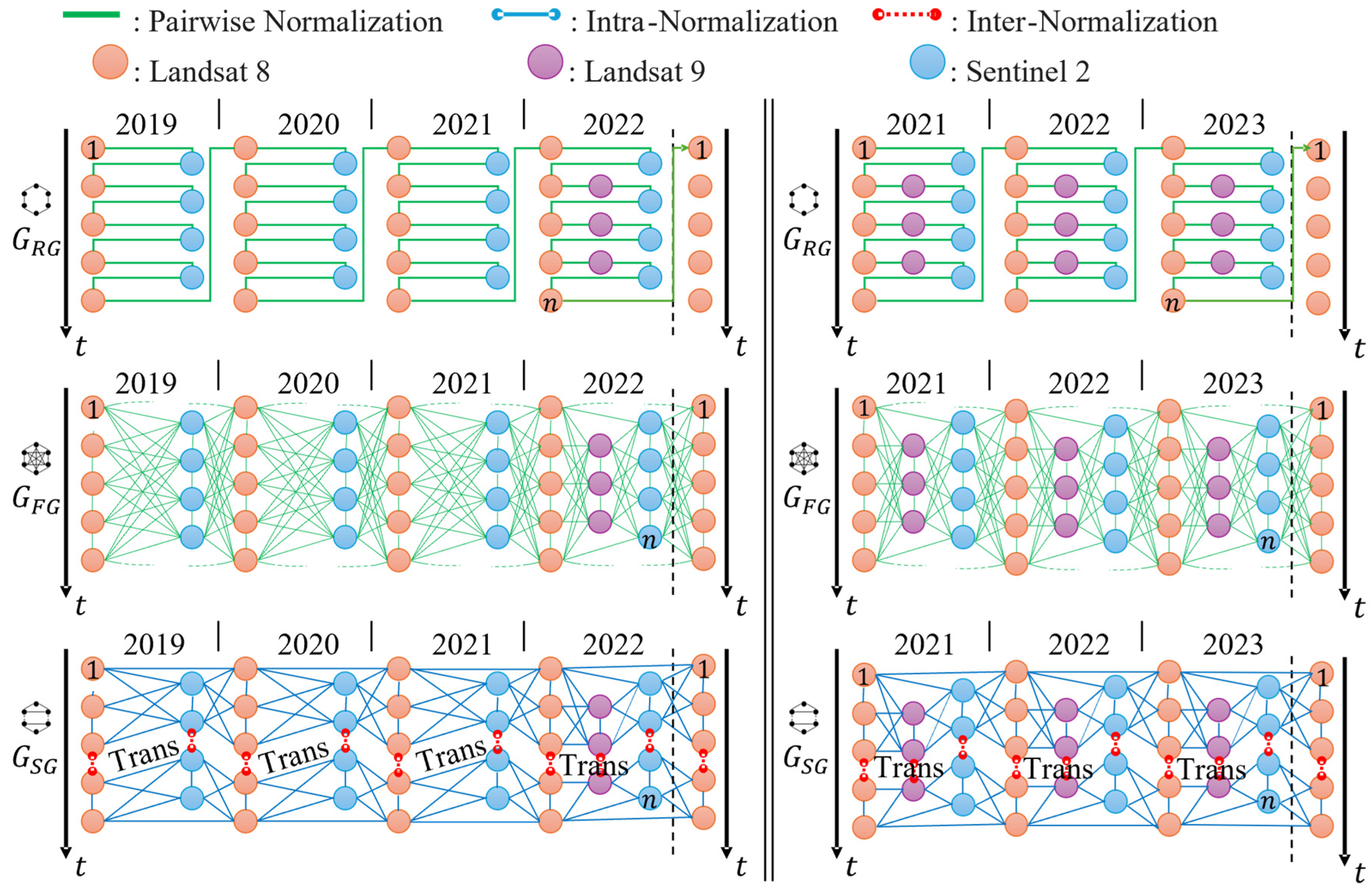
Three graph structures were employed in this study for the test datasets BR and TW and are shown in Figure 5. The normalization graphs are ring graph $G_{RG}$, fully connected graph $G_{FG}$, and season-aware graph $G_{SG}$. In ring graph $G_{RG}$, each image is connected to its immediate temporal neighbors. By limiting normalization to local relationships, it encourages smooth changes between adjacent acquisition dates while maintaining low computational complexity [36]. In contrast, fully connected graph $G_{FG}$ establishes links each image to all the other images in a dataset. This configuration leverages the complete set of reflectance relationships, promoting stronger global temporal consistency across the entire time series, though at significantly higher computational cost.

Figure 5. Graph structures of the test datasets BR (left) and TW (right). From top to bottom: ring graph $G_{RG}$, fully connected graph $G_{FG}$, and season-aware graph $G_{SG}$.

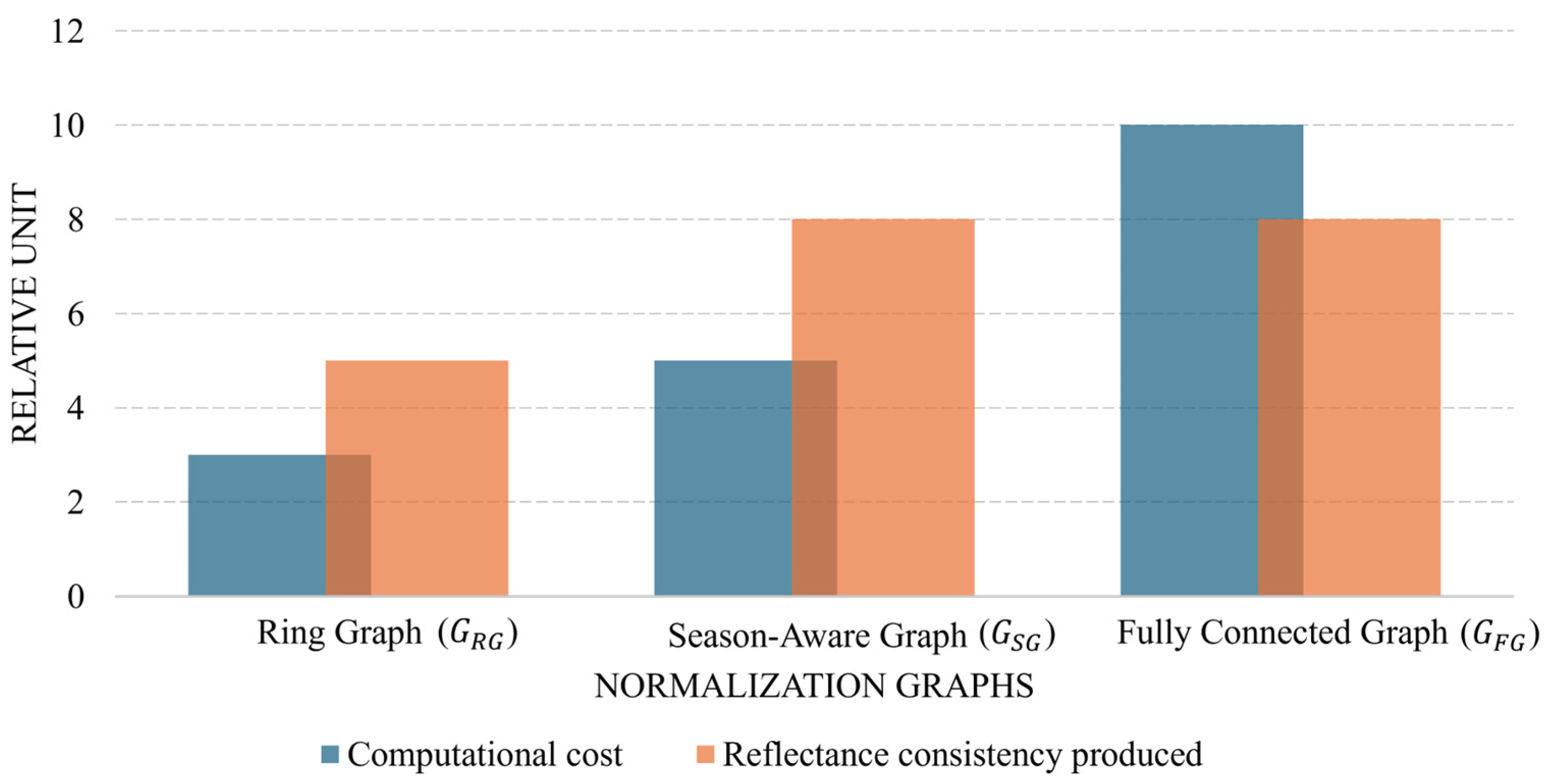
To address the limitations of those two conventional structures, we introduce the season-aware graph, $G_{SG}$. This graph incorporates seasonal similarities into its structure, enabling a design that reduces the computational cost of a fully connected graph while achieving higher reflectance consistency than a ring graph (Figure 6). The images are first sorted into seasonally consistent subsets based on temporal consistency across the entire time series. Then, normalization proceeds in two stages, inter-normalization and inter-normalization. Inter-normalization adjusts the reflectance of transition images between image groups to prevent seasonal drift. Intra-normalization refines reflectance consistency within each seasonal group. The subgraph for each instance of intra-normalization can be ring graph $G_{RG}$ or fully connected graph $G_{FG}$. In this study, the $G_{FG}$ subgraph is utilized for intra-normalization, a choice made to maximize radiometric information sharing and enforce the strongest possible consensus within each seasonal group, thereby demonstrating the full capability of the weighted normalization strategy. This architecture, using the densest internal subgraph, is called the $G_{FG}$-based season-aware graph.

Figure 6. Comparison of relative computational cost and reflectance consistency between ring graph $G_{RG}$ or fully connected graph $G_{FG}$ and proposed season-aware graph $G_{SG}$.

3.2. Visual Assessment of Graph-Based Reflectance Normalization

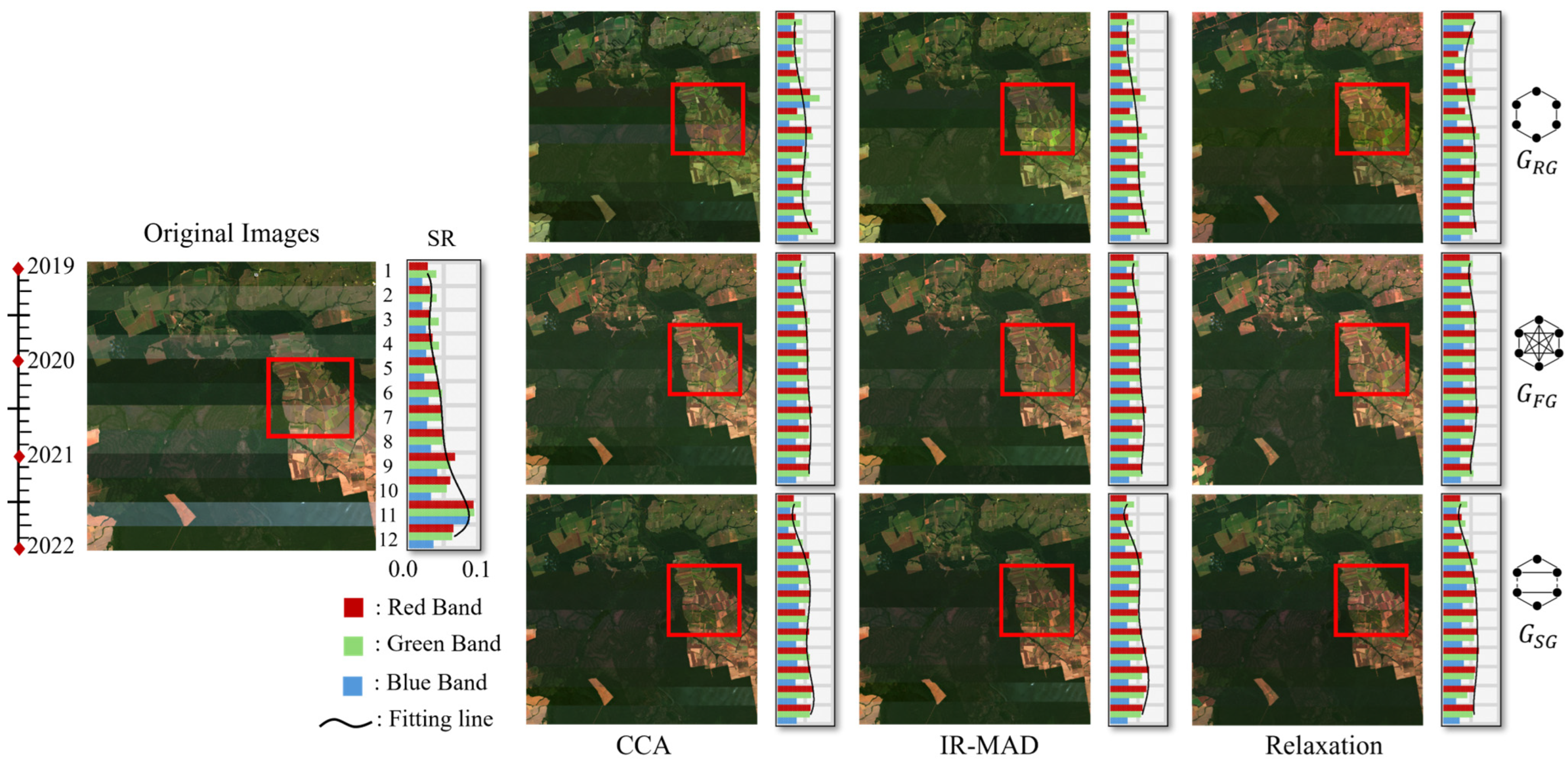
The normalization results of using the methods CCA [39], IR-MAD [31], and relaxation [36] on the dataset BR are shown in Figure 7. These methods were selected as foundational RRN benchmarks to explicitly test and isolate the structural contribution of the three graph structures ($G_{RG}$, $G_{FG}$, and $G_{SG}$) from the underlying normalization workflow. When using the ring graph $G_{RG}$, all methods successfully reduced extreme reflectance values; however, both CCA and IR-MAD produced noticeable inconsistencies between consecutive images. The resulting temporal discontinuity is evident in their spectral profiles, which display abrupt shifts at image boundaries. In practice, this under-normalization (Figure 7, Top Row) introduces edge effects in downstream analysis, where the detected change is an artifact of the normalization boundary, not a real environmental event.

Figure 7. Comparisons of reflectance normalization using different graph structures: ring graph ($G_{RG}$), fully connected graph ($G_{FG}$), and proposed season-aware graph ($G_{SG}$). Left: Twelve raw satellite images (Image 1 to Image 12) from BR dataset containing the red, green, and blue bands; Right: reflectance normalization results using CCA, IR-MAD, and relaxation-based normalization.

When using the fully connected graph $G_{FG}$, all three normalization methods produced highly consistent reflectance values across the dataset. However, the normalized images became almost indistinguishable from one another, regardless of seasonal or temporal variation. This effect is further confirmed by the spectral profiles, which appear overly smooth and lack expected seasonal fluctuations. The excessive suppression of temporal variability suggests that $G_{FG}$ leads to over-normalization (Figure 7, Middle Row), limiting its applicability for long-term environmental monitoring where natural change detection is essential.

In contrast, the proposed season-aware graph preserved distinct seasonal characteristics while ensuring smooth transition between wet and dry periods. The normalization results retained meaningful spectral variation without introducing abrupt shifts. This demonstrates that $G_{SG}$ strikes an effective balance between temporal consistency and seasonal distinctiveness. Additionally, the combination of $G_{SG}$ with the relaxation-based normalization yielded the most stable normalization outcomes, confirming its advantage due to its structurally optimized architecture in mitigating temporal inconsistency while maintaining seasonal integrity.

3.3. Statistical Assessment of Graph-Based Reflectance Normalization

To evaluate the performance of the normalization methods, three statistical metrics were employed: mean absolute error (MAE), root mean squared error (RMSE), and SSIM. MAE and RMSE quantify the overall magnitude of errors and help identify outliers in the normalization process. These metrics are calculated by comparing the differences between the normalized images with their corresponding reference images, which enables the assessment of how well the method preserves seasonal characteristics and maintains temporal reflectance consistency.

As shown in Table 2, the normalization methods using the ring graph ($G_{RG}$) resulted in relatively higher MAE and RMSE values, particularly for images captured during seasonal transitions. This limitation is attributed to the sparse connectivity of the ring structure, where insufficient cross-season information leads to error accumulation and propagation between temporally adjacent images. The fully connected graph ($G_{FG}$) achieved lower MAEs and RMSEs, indicating improved reflectance consistency due to its dense connectivity. However, this extensive linkage also introduces a tendency toward over-normalization, where seasonal variations are suppressed and unique temporal characteristics are diminished. In contrast, the season-aware graph ($G_{SG}$) consistently outperformed both $G_{RG}$ and $G_{FG}$, achieving the lowest error values across almost all test cases. Notably, when paired with the relaxation-based normalization, $G_{SG}$ yielded the best overall performance, producing minimal errors for both seasonal groups and transition images. These results confirm that relaxation-based normalization using the season-aware graph effectively preserves seasonal identity while minimizing reflectance discrepancies and maintaining temporal coherence.

Table 2. Accuracy assessments of reflectance normalization through the normalization graphs $G_{RG}$, $G_{FG}$, and $G_{SG}$. The metrics MAE and RMSE are used.

MAE/RMSE	CCA
	Wet Seasons	Transitions	Dry Seasons
Original Image	0.557/0.198	0.605/0.206	0.994/0.231
$G_{RG}$	0.474/0.170	1.144/0.286	0.727/0.220
$G_{FG}$	0.465/0.164	0.483/0.177	0.475/0.174
$G_{SG}$	0.465/0.165	0.497/0.177	0.469/0.166
MAE/RMSE	IR-MAD
	Wet Seasons	Transitions	Dry Seasons
Original Image	0.557/0.198	0.605/0.206	0.994/0.231
$G_{RG}$	0.481/0.167	0.769/0.208	0.690/0.198
$G_{FG}$	0.473/0.160	0.479/0.161	0.473/0.161
$G_{SG}$	0.468/0.160	0.486/0.166	0.470/0.158
MAE/RMSE	Relaxation-Based
	Wet Seasons	Transitions	Dry Seasons
Original Image	0.557/0.198	0.605/0.206	0.994/0.231
$G_{RG}$	0.484/0.185	0.759/0.217	0.630/0.214
$G_{FG}$	0.457/0.158	0.461/0.160	0.456/0.158
$G_{SG}$	0.453/0.157	0.461/0.160	0.446/0.144

Subsequently, SSIM was employed to assess how well the normalization method preserves the structural integrity of the images relative to reference images. Table 3 presents the SSIM scores of the graphs $G_{RG}$, $G_{FG}$, and $G_{SG}$ with the normalization methods CCA, IR-MAD, and the relaxation-based algorithm. The normalization performed with $G_{RG}$ consistently produced the lowest SSIM values, especially for images captured during dry seasons and transitional periods. This degradation can be attributed to abrupt reflectance variations and the absence of seasonal continuity within the graph, leading to insufficient information propagation between nonadjacent temporal neighbors. In contrast, normalization using $G_{FG}$ yields noticeably higher SSIMs across all seasons. Notably, during seasonal transitions, $G_{FG}$ slightly surpasses $G_{SG}$, likely due to their dense interconnections that can lead to over-normalization. Nonetheless, the overall results demonstrate that normalization with the proposed $G_{SG}$ achieves the most stable and consistent performance, outperforming both $G_{RG}$ and $G_{FG}$. In particular, relaxation-based normalization paired with $G_{SG}$ achieves the highest SSIM (0.935 for dry-season images), reinforcing the effectiveness of the proposed graph for reliable long-term monitoring using multi-sensor and multi-temporal satellite imagery.

Table 3. Similarity after normalization comparisons between the graphs $G_{RG}$, $G_{FG}$, and $G_{SG}$ using the SSIM.

SSIM	CCA
	Wet Seasons	Transitions	Dry Seasons
Original Image	0.79	0.876	0.907
$G_{RG}$	0.835	0.832	0.873
$G_{FG}$	0.836	0.878	0.913
$G_{SG}$	0.868	0.877	0.931
SSIM	IR-MAD
	Wet Seasons	Transitions	Dry Seasons
Original Image	0.79	0.876	0.907
$G_{RG}$	0.829	0.846	0.863
$G_{FG}$	0.837	0.879	0.913
$G_{SG}$	0.843	0.878	0.930
SSIM	Relaxation-Based
	Wet Seasons	Transitions	Dry Seasons
Original Image	0.79	0.876	0.907
$G_{RG}$	0.825	0.844	0.883
$G_{FG}$	0.852	0.878	0.916
$G_{SG}$	0.856	0.880	0.935

3.4. Comparisons of NDVIs from Normalized Images

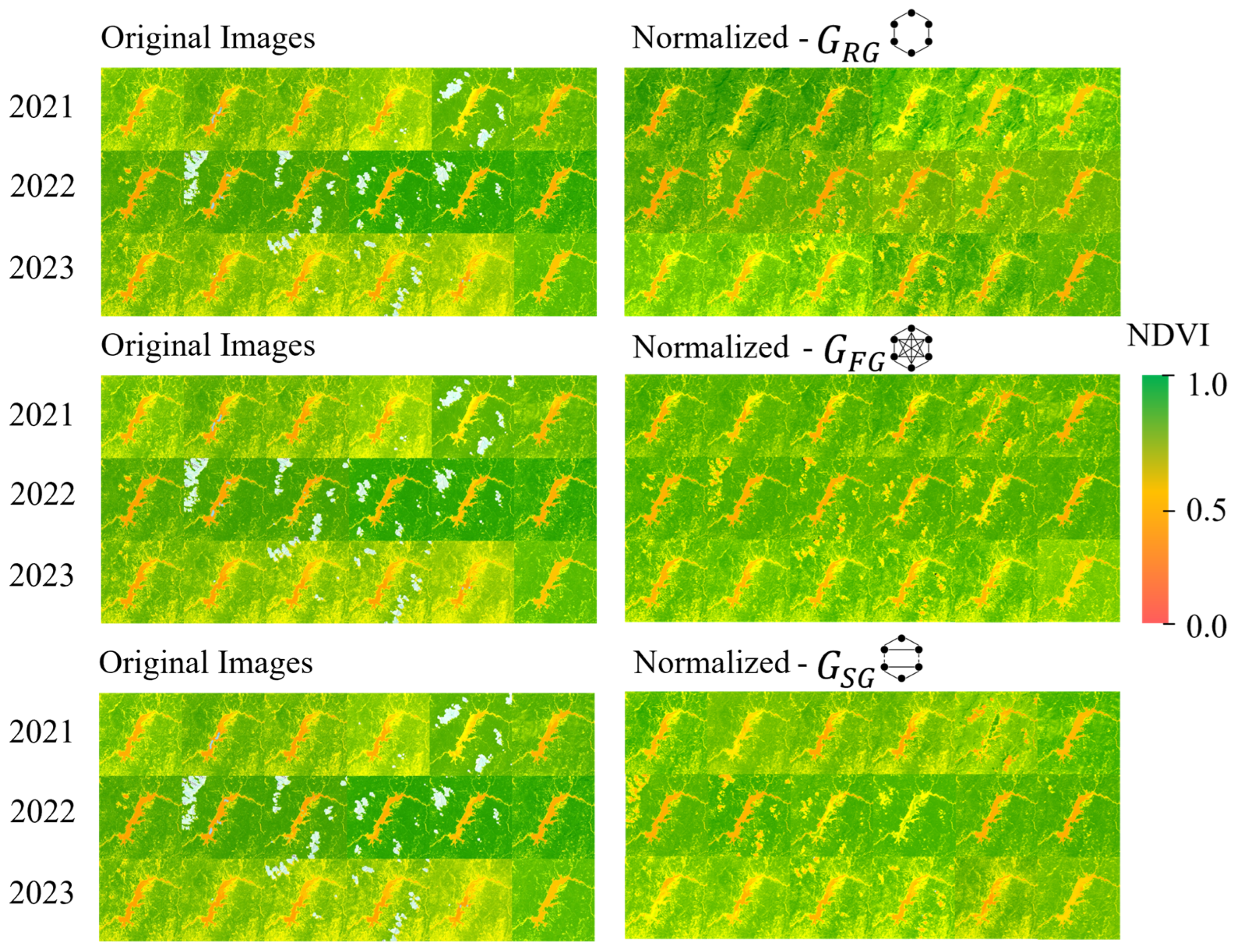
The comparisons of the NDVIs of the normalized image are shown in Figure 8. The images were normalized using relaxation-based reflectance normalization with different graph structures, and the dataset TW is used in the experiment. The NDVIs of the $G_{RG}$-based normalized images exhibit local consistency but fail to preserve seasonal characteristics. This issue is because of inadequate handling of seasonal transition periods during normalization, which leads to reflectance inconsistencies and distortion of temporal patterns. As for the $G_{FG}$-based normalization, the NDVIs of the normalized images are visually uniform across seasons, benefiting from its full-connected graph structure. This visual uniformity can benefit short-term monitoring. However, this visually uniform appearance comes at the practical cost of over-normalization, which suppresses seasonal transitions, making the data unsuitable for capturing seasonal dynamics in long-term monitoring. In contrast, the NDVIs of the $G_{SG}$-based normalized images achieve balanced results in which seasonal identities are preserved and smooth inter-seasonal transitions are maintained.

Figure 8. NDVI comparison using Taiwan dataset. Left: The raw NDVIs obtained from the original satellite images. Right: The NDVIs of the relaxation-based normalized images.

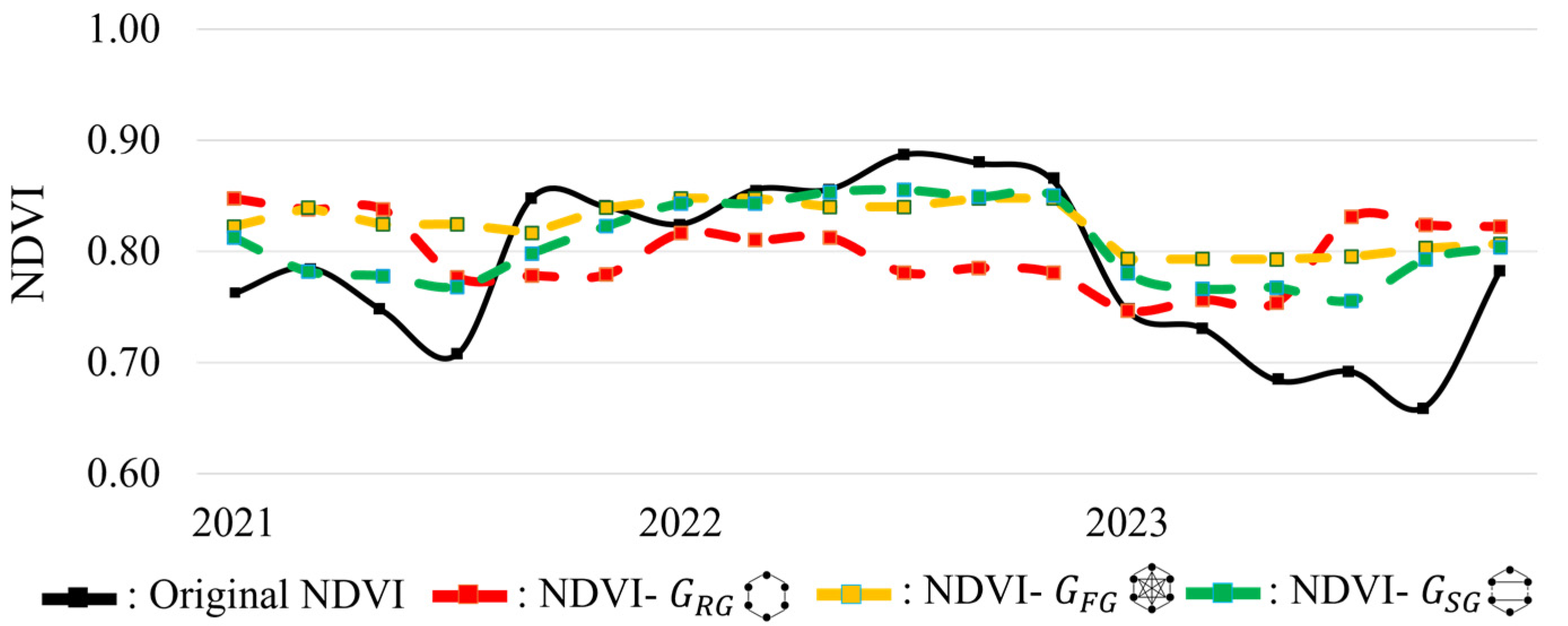
The NDVI temporal variations before and after reflectance normalization using the graph structures $G_{RG}$, $G_{FG}$, and $G_{SG}$ are further presented in Figure 9. The dataset TW is tested, and the averages of NDVI images acquired from 2021 to 2023 are utilized to show the temporal NDVI trends. The raw NDVIs (Figure 9—black) obtained from the original satellite images exhibit significant temporal fluctuations, which reveal reflectance temporal inconsistency. With reflectance normalization, reflectance temporal inconsistency is alleviated. However, abrupt NDVI changes and local consistency occur in the NDVIs after normalization with the graph $G_{RG}$, as shown in Figure 9—red. In contrast, normalization with the graph $G_{FG}$ achieves excellent NDVI consistency, as shown in Figure 9—yellow. However, this consistency tends to suppress seasonal variations, producing overly smoothed NDVI trends that may obscure some environmental changes. Normalization with the graph $G_{SG}$ offers a balanced result, maintaining globally temporal reflectance consistency and local temporal fidelity by avoiding the artificial flatness of $G_{FG}$ and the spikes of $G_{RG}$. It confirms the practical advantage of graph-based relaxation which ensures that genuine environmental anomalies (like a drought period) are preserved and not artificially smoothed.

Figure 9. NDVI temporal trends before and after relaxation-based reflectance normalization with the graphs $G_{RG}$ (denoted by red), $G_{FG}$ (denoted by yellow), and $G_{SG}$ (denoted by green). The black solid line represents the original NDVI trend.

4. Conclusions

This study introduces graph-based relaxation for reflectance normalization of cross-sensor and multi-temporal satellite imagery. Three graph structures, that is, a ring graph, fully connected graph, and season-aware graph, are utilized. In experiments, two image datasets from Landsat 8, Landsat 9, and Sentinel 2 are tested. The experimental results show that relaxation-based reflectance normalization with a season-aware graph can reduce the possibilities of over- and under-normalization, and the normalization performance is better than that of the related methods, CCA and IR-MAD. The qualitative results confirmed the method’s ability to maintain seasonal identity and preserve gradual environmental changes without abrupt shifts. The quantitative analyses using MAE, RMSE, and SSIM further validated the graph-based relaxation performance while the NDVI temporal analysis demonstrated its strength in maintaining meaningful seasonal variations with local and global consistency. These findings conclude that reflectance relaxation with the season-aware graph can be applied to short-term and long-term environmental monitoring. Since IR-MAD and linear regression are multi-band methods, the proposed framework is theoretically applicable to hyperspectral data. Adaptation for SAR time series requires replacing the IR-MAD/Regression base with a SAR-appropriate RRN technique and modifying the grouping metrics NDVI and SSIM to a SAR-specific temporal coherence metric. In future work, the proposed framework will be further validated by expanding its application range and incorporating additional indices such as the Enhanced Vegetation Index (EVI) and the Normalized Burn Ratio (NBR), strengthening its relevance for vegetation assessment, disturbance mapping, and ecosystem monitoring. Beyond these extensions, the season-aware graph offers a structured foundation for integration with machine learning-based normalization frameworks. Embedding the graph topology into models such as Graph Neural Networks would allow the system to learn non-linear, season-dependent reflectance behaviors while retaining the physically interpretable constraints of the graph. This direction provides a concrete pathway toward a more automated and scalable normalization strategy for large, multi-sensor and multi-temporal Earth-observation datasets.

References

- Smith, G.M.; Milton, E.J. The Use of the Empirical Line Method to Calibrate Remotely Sensed Data to Reflectance. Int. J. Remote Sens. 1999, 20, 2653–2662. [Google Scholar] [CrossRef]
- Hemingway, B.L.; Frazier, A.E. Cross-Sensor Radiometric Normalization of Planet Smallsat Data Using Sentinel-2 to Improve Consistency across Scenes and Environments. In Proceedings of the Image and Signal Processing for Remote Sensing XXVII, Online, Spain, 12 September 2021; Bruzzone, L., Bovolo, F., Benediktsson, J.A., Eds.; SPIE: Bellingham, WA, USA, 2021; p. 1186204. [Google Scholar]
- Broncano-Mateos, C.J.; Pinilla, C.; Gonzalez-Crespo, R.; Castillo-Sanz, A. Relative Radiometric Normalization of Multitemporal Images. IJIMAI 2010, 1, 53. [Google Scholar] [CrossRef]
- Anees, S.A.; Zhang, X.; Shakeel, M.; Al-Kahtani, M.A.; Khan, K.A.; Akram, M.; Ghramh, H.A. Estimation of Fractional Vegetation Cover Dynamics Based on Satellite Remote Sensing in Pakistan: A Comprehensive Study on the FVC and Its Drivers. J. King Saud Univ.—Sci. 2022, 34, 101848. [Google Scholar] [CrossRef]
- Asokan, A.; Anitha, J. Change Detection Techniques for Remote Sensing Applications: A Survey. Earth Sci. Inf. 2019, 12, 143–160. [Google Scholar] [CrossRef]
- Han, H.; Liu, Z.; Li, J.; Zeng, Z. Challenges in Remote Sensing Based Climate and Crop Monitoring: Navigating the Complexities Using AI. J. Cloud Comp. 2024, 13, 34. [Google Scholar] [CrossRef]
- Hu, Y.; Liu, L.; Liu, L.; Jiao, Q. Comparison of absolute and relative radiometric normalization use Landsat time series images. In Proceedings of the Comparison of Absolute and Relative Radiometric Normalization Use Landsat Time Series Images, Guilin, China, 20 November 2011; Liu, J., Tian, J., Sang, H., Ma, J., Eds.; IEEE: New York, NY, USA, 2011; p. 800616. [Google Scholar]
- Farhad, M.M.; Kaewmanee, M.; Leigh, L.; Helder, D. Radiometric Cross Calibration and Validation Using 4 Angle BRDF Model between Landsat 8 and Sentinel 2A. Remote Sens. 2020, 12, 806. [Google Scholar] [CrossRef]
- Anderson, G.P.; Felde, G.W.; Hoke, M.L.; Ratkowski, A.J.; Cooley, T.W.; Chetwynd, J.H., Jr.; Gardner, J.A.; Adler-Golden, S.M.; Matthew, M.W.; Berk, A.; et al. MODTRAN4-based atmospheric correction algorithm: FLAASH (fast line-of-sight atmospheric analysis of spectral hypercubes). In Proceedings of the MODTRAN4-Based Atmospheric Correction Algorithm: FLAASH (Fast Line-of-Sight Atmospheric Analysis of Spectral Hypercubes), Orlando, FL, USA, 1 August 2002; Shen, S.S., Lewis, P.E., Eds.; Exelis Visual Information Solutions: McLean, WV, USA, 2002; pp. 65–71. [Google Scholar]
- Maher, A. Evaluation of Atmospherically Gases Using Models FLAASH and QUAC to Hyper-Spectral Imagery. Karbala Int. J. Mod. Sci. 2019, 5, 3. [Google Scholar] [CrossRef]
- Hawes, F.T.; Berk, A.; Van Den Bosch, J.; Fortin, G. MODTRAN7: A Polarimetric Extension of the MODTRAN6 Radiometric Atmospheric Radiative Transfer Model. In Proceedings of the Polarization: Measurement, Analysis, and Remote Sensing XV, Orlando, FL, USA, 3–7 April 2022; Chenault, D.B., Kupinski, M.K., Eds.; SPIE: Bellingham, WA, USA, 2022; p. 9. [Google Scholar]
- Jasso-Garduño, A.E.; Muñoz-Máximo, I.; Pinto, D.; Ramírez-Cortés, J.M. Deep Learning Based Emulation of Radiative Transfer Code for Atmospheric Correction of Satellite Images. CyS 2024, 28, 2327–2341. [Google Scholar] [CrossRef]
- Bassani, C.; Manzo, C.; Zakey, A.; Cuevas-Agulló, E. Effect of the Aerosol Type Selection for the Retrieval of Shortwave Ground Net Radiation: Case Study Using Landsat 8 Data. Atmosphere 2016, 7, 111. [Google Scholar] [CrossRef]
- de Carvalho, O.; Guimarães, R.; Silva, N.; Gillespie, A.; Gomes, R.; Silva, C.; de Carvalho, A. Radiometric Normalization of Temporal Images Combining Automatic Detection of Pseudo-Invariant Features from the Distance and Similarity Spectral Measures, Density Scatterplot Analysis, and Robust Regression. Remote Sens. 2013, 5, 2763–2794. [Google Scholar] [CrossRef]
- Moghimi, A.; Celik, T.; Mohammadzadeh, A.; Kusetogullari, H. Comparison of Keypoint Detectors and Descriptors for Relative Radiometric Normalization of Bitemporal Remote Sensing Images. IEEE J. Sel. Top. Appl. Earth Obs. Remote Sens. 2021, 14, 4063–4073. [Google Scholar] [CrossRef]
- Rayegani, B.; Barati, S.; Sarkheil, H. A Simple Model for PIFs Extraction at Digital Change Detection Approach. Model. Earth Syst. Environ. 2021, 7, 1769–1781. [Google Scholar] [CrossRef]
- Chen, L.; Ma, Y.; Lian, Y.; Zhang, H.; Yu, Y.; Lin, Y. Radiometric Normalization Using a Pseudo−Invariant Polygon Features−Based Algorithm with Contemporaneous Sentinel−2A and Landsat−8 OLI Imagery. Appl. Sci. 2023, 13, 2525. [Google Scholar] [CrossRef]
- Bai, Y.; Tang, P.; Hu, C. kCCA Transformation-Based Radiometric Normalization of Multi-Temporal Satellite Images. Remote Sens. 2018, 10, 432. [Google Scholar] [CrossRef]
- Denaro, L.G.; Lin, C.-H. Hybrid Canonical Correlation Analysis and Regression for Radiometric Normalization of Cross-Sensor Satellite Imagery. IEEE J. Sel. Top. Appl. Earth Obs. Remote Sens. 2020, 13, 976–986. [Google Scholar] [CrossRef]
- Ding, H.; Shi, J.; Wang, Y.; Wei, L. An improved dark-object subtraction technique for atmospheric correction of Landsat 8. In Proceedings of the An Improved Dark-Object Subtraction Technique for Atmospheric Correction of Landsat 8, Enshi, China, 14 December 2015; Liu, J., Sun, H., Eds.; SPIE: Bellingham, WA, USA, 2015; p. 98150K. [Google Scholar]
- Nicolau, R.; Basos, N.; Marcelino, F.; Caetano, M.; Pereira, J.M.C. Harmonization of Categorical Maps by Alignment Processes and Thematic Consistency Analysis. AIMS Geosci. 2020, 6, 473–490. [Google Scholar] [CrossRef]
- Yu, X.; Fan, J.; Zhang, M.; Liu, Q.; Li, Y.; Zhang, D.; Zhou, Y. Relative Radiation Correction Based on CycleGAN for Visual Perception Improvement in High-Resolution Remote Sensing Images. IEEE Access 2021, 9, 106627–106640. [Google Scholar] [CrossRef]
- Sambandham, V.T.; Kirchheim, K.; Ortmeier, F.; Mukhopadhaya, S. Deep Learning-Based Harmonization and Super-Resolution of Landsat-8 and Sentinel-2 Images. ISPRS J. Photogramm. Remote Sens. 2024, 212, 274–288. [Google Scholar] [CrossRef]
- Liu, S.; Wang, L.; Lian, J.; Liu, C.; Zhan, X.; Liu, J.; Wang, T.; Geng, D.; Duan, H.; Zou, S. Auto-Robust Relative Radiometric Normalization via Latent Change Noise Modeling. IEEE Trans. Geosci. Remote Sens. 2024, 62, 1–15. [Google Scholar] [CrossRef]
- Koczkodaj, W.W.; Magnot, J.-P.; Mazurek, J.; Peters, J.F.; Rakhshani, H.; Soltys, M.; Strzałka, D.; Szybowski, J.; Tozzi, A. On Normalization of Inconsistency Indicators in Pairwise Comparisons. Int. J. Approx. Reason. 2017, 86, 73–79. [Google Scholar] [CrossRef]
- Wu, W.; Sun, X.; Wang, X.; Fan, J.; Luo, J.; Shen, Y.; Yang, Y. A Long Time-Series Radiometric Normalization Method for Landsat Images. Sensors 2018, 18, 4505. [Google Scholar] [CrossRef]
- Wilson, R.J. Introduction to Graph Theory, 4th ed.; Nachdr; Prentice Hall: Harlow, UK; Munich, Germany, 2009; ISBN 978-0-582-24993-6. [Google Scholar]
- Ghanbari, H.; Homayouni, S.; Ghamisi, P.; Safari, A. Radiometric Normalization of Multitemporal and Multisensor Remote Sensing Images Based on a Gaussian Mixture Model and Error Ellipse. IEEE J. Sel. Top. Appl. Earth Obs. Remote Sens. 2018, 11, 4526–4533. [Google Scholar] [CrossRef]
- Chen, Y. Improved Relative Radiometric Normalization Method of Remote Sensing Images for Change Detection. J. Appl. Rem. Sens. 2018, 12, 045018. [Google Scholar] [CrossRef]
- Gan, W.; Albanwan, H.; Qin, R. Radiometric Normalization of Multitemporal Landsat and Sentinel-2 Images Using a Reference MODIS Product Through Spatiotemporal Filtering. IEEE J. Sel. Top. Appl. Earth Obs. Remote Sens. 2021, 14, 4000–4013. [Google Scholar] [CrossRef]
- Canty, M.J.; Nielsen, A.A. Automatic Radiometric Normalization of Multitemporal Satellite Imagery with the Iteratively Re-Weighted MAD Transformation. Remote Sens. Environ. 2008, 112, 1025–1036. [Google Scholar] [CrossRef]
- Marpu, P.R.; Gamba, P.; Canty, M.J. Improving Change Detection Results of IR-MAD by Eliminating Strong Changes. IEEE Geosci. Remote Sens. Lett. 2011, 8, 799–803. [Google Scholar] [CrossRef]
- Barazzetti, L.; Gianinetto, M.; Scaioni, M. Radiometric normalization with multi-image pseudo-invariant features. In Proceedings of the Radiometric Normalization with Multi-Image Pseudo-Invariant Features, Paphos, Cyprus, 12 August 2016; Themistocleous, K., Hadjimitsis, D.G., Michaelides, S., Papadavid, G., Eds.; IEEE: New York, NY, USA, 2016; p. 968807. [Google Scholar]
- Nielsen, A.A. The Regularized Iteratively Reweighted MAD Method for Change Detection in Multi- and Hyperspectral Data. IEEE Trans. Image Process. 2007, 16, 463–478. [Google Scholar] [CrossRef]
- Wang, B.; Choi, S.-K.; Han, Y.-K.; Lee, S.-K.; Choi, J.-W. Application of IR-MAD Using Synthetically Fused Images for Change Detection in Hyperspectral Data. Remote Sens. Lett. 2015, 6, 578–586. [Google Scholar] [CrossRef]
- Ryadi, G.Y.I.; Syariz, M.A.; Lin, C.-H. Relaxation-Based Radiometric Normalization for Multitemporal Cross-Sensor Satellite Images. Sensors 2023, 23, 5150. [Google Scholar] [CrossRef]
- Sabino, M.; Da Silva, A.C.; De Almeida, F.T.; De Souza, A.P. Reference Evapotranspiration in Climate Change Scenarios in Mato Grosso, Brazil. Hydrology 2024, 11, 91. [Google Scholar] [CrossRef]
- Commar, L.F.S.; Louzada, L.; Costa, M.H.; Brumatti, L.M.; Abrahão, G.M. Mato Grosso’s Rainy Season: Past, Present, and Future Trends Justify Immediate Action. Environ. Res. Lett. 2024, 19, 114065. [Google Scholar] [CrossRef]
- Dunlap, W.P.; Brody, C.J.; Greer, T. Canonical Correlation and Chi-Square: Relationships and Interpretation. J. Gen. Psychol. 2000, 127, 341–353. [Google Scholar] [CrossRef] [PubMed]
Disclaimer/Publisher’s Note: The statements, opinions and data contained in all publications are solely those of the individual author(s) and contributor(s) and not of MDPI and/or the editor(s). MDPI and/or the editor(s) disclaim responsibility for any injury to people or property resulting from any ideas, methods, instructions or products referred to in the content. |
© 2025 by the authors. Licensee MDPI, Basel, Switzerland. This article is an open access article distributed under the terms and conditions of the Creative Commons Attribution (CC BY) license (https://creativecommons.org/licenses/by/4.0/).