Highlights
- What are the main findings?
- The study shows that while traditional gap-filling methods like Kriging and SG Filtering perform well with small data gaps, their accuracy diminishes when the missing data is extensive or the environment is dynamic. However, such conditions are quite common in inland lakes.
- DINEOF and DINCAE outperform in capturing spatiotemporal variability, maintaining high accuracy even with over 60% missing data, making them suitable for eutrophic lake across cloudy-rainy regions.
- What are the implications of the main findings?
- The data reconstruction method can be used to generate spatiotemporal seamless datasets, enhancing the accuracy and completeness of lake water quality monitoring data and enabling a more precise capture of dynamic changes in lakes.
- The spatiotemporal seamless reconstructed data can provide crucial data support for practical applications, such as short-term forecasting of lake water color parameters, addressing the issue of data scarcity in lake management.
Abstract
Satellite remote sensing is an important approach for monitoring lake water environments. However, in regions with frequent cloud and rainfall, optical remote sensing imagery often suffers from extensive data gaps caused by cloud cover, rainfall, and sun glint, which severely limit its continuity and reliability for long-term monitoring. To address this issue, this study uses Lake Taihu—a typical eutrophic lake located in a cloudy and rainy region—as a case study and systematically compares four representative gap-filling methods: Kriging Interpolation, Savitzky–Golay (SG) Filtering, Data Interpolating Empirical Orthogonal Functions (DINEOF), and the Data Interpolating Convolutional Auto Encoder (DINCAE). The results show that traditional methods retain some accuracy under low missing-data conditions (for Kriging: R = 0.84, RMSE = 7.85 μg/L; for SG Filtering: R = 0.88, RMSE = 6.67 μg/L), but tend to produce over-smoothing or distorted estimations in cases of extensive gaps or highly dynamic environments. In contrast, both DINEOF and DINCAE capture the spatiotemporal variability of chlorophyll-a more effectively, maintaining relatively high accuracy and robustness even when the missing rate exceeds 60% (for DINEOF: R = 0.84, RMSE = 6.91 μg/L; for DINCAE: R = 0.79, RMSE = 8 μg/L). Based on the optimal algorithm, a seamless long-term dataset of chlorophyll-a concentration covering Lake Taihu can be constructed, providing a solid data foundation for eutrophication trend analysis and algal bloom early warning. This study demonstrates the effectiveness of integrating statistical and deep learning approaches for lake water color remote sensing data reconstruction, offering important implications for enhancing continuous monitoring of lake water environments and supporting ecological management decisions.
1. Introduction
Lakes are vital repositories of freshwater resources, playing an irreplaceable role in sustaining global biodiversity, safeguarding drinking water security, and regulating climate. In addition, they provide multiple ecosystem services and socioeconomic functions, including flood control and water storage, aquaculture, navigation, irrigation, and industrial production [,]. Yet, under the combined pressures of human activities and global climate change, many lakes worldwide are experiencing rapid water quality deterioration, increasingly frequent cyanobacterial blooms, and the degradation of aquatic vegetation [,], thereby posing serious threats to lake ecosystem health [].
Chlorophyll-a (Chl-a) concentration is a key indicator of eutrophication and has been widely employed in water quality assessment []. Conventional monitoring methods, however, typically rely on field sampling and laboratory analysis, which are costly, labor-intensive, and spatially constrained. In contrast, satellite remote sensing enables efficient and large-scale acquisition of the spatiotemporal distribution of Chl-a [,]. Moreover, it provides essential initial conditions for simulating and forecasting cyanobacterial blooms and has already become a critical tool in water quality monitoring and algal bloom early-warning applications [].
Nonetheless, optical remote sensing data are frequently compromised by cloud cover, rainfall, and other adverse conditions, leading to substantial gaps and reduced data quality [,]. Globally, the proportion of missing data in Landsat imagery is estimated to be around 40% []. The issue is even more pronounced in persistently cloudy and rainy regions: for example, in the middle and lower reaches of the Yangtze River, the average missing rate during the rainy season exceeds 60% []. Such gaps not only undermine the completeness and reliability of remote sensing datasets but may also result in misinterpretation of critical regime shifts in long-term analyses []. Furthermore, missing data can degrade the performance of bloom forecasting and early-warning models that rely on remote sensing as initial conditions, limiting their operational utility []. Consequently, developing effective approaches to reconstruct missing observations and generate seamless spatiotemporal remote sensing datasets has become an urgent priority in water color remote sensing research.
Methods for reconstructing missing remote sensing data can generally be categorized into three groups: spatial interpolation methods, temporal interpolation methods, and spatiotemporal fusion approaches []. Spatial interpolation methods rely on the spatial continuity of pixels in remote sensing imagery, estimating missing regions using information from neighboring pixels. Common techniques include Nearest Neighbor interpolation [], Bilinear Interpolation [], Inverse Distance Weighting [], and Kriging Interpolation []. Temporal interpolation methods, specifically, exploit the temporal dynamics of observed data, reconstructing missing values using information from historical observations. Representative approaches include Regression Analysis [], Time-series Fusion [], Temporal Weighted Averaging [], and Savitzky–Golay (SG) Filtering []. While these methods are effective for certain reconstruction tasks, their accuracy and applicability remain limited in scenarios involving large-scale or consecutive data gaps [].
In recent years, spatiotemporal reconstruction methods have been proposed to improve robustness and accuracy by simultaneously leveraging spatial and temporal information. Notable examples include the Data Interpolating Empirical Orthogonal Functions (DINEOF), grounded in statistical methods [], and the Data Interpolating Convolutional Auto Encoder (DINCAE), developed within the deep learning framework []. These approaches jointly model spatiotemporal dynamics during reconstruction and have demonstrated superior performance in oceanic and terrestrial remote sensing applications []. However, compared with these broader contexts, inland lakes are generally characterized by smaller spatial scales, higher spatial heterogeneity, and more pronounced spatiotemporal variability [], raising questions about the suitability and performance of such methods in reconstructing lake water color parameters.
This study takes Lake Taihu—a typical eutrophic lake situated in a cloudy and rainy region—as a case study to evaluate the applicability and performance of different reconstruction algorithms for inland lake water color remote sensing data. Firstly, we systematically assess Kriging, SG Filtering, DINEOF, and DINCAE, focusing on their reconstruction performance under frequent cloud–rain observation conditions and the optically complex characteristics of inland waters. Secondly, based on this evaluation, the optimal algorithm is selected to generate a seamless spatiotemporal dataset of water quality parameters for Lake Taihu. Finally, the outcomes of this study are expected to provide an efficient and reliable solution for reconstructing water color remote sensing parameters in cloudy and rainy lake regions, enhance the continuity and accuracy of monitoring results, and ultimately offer scientific data support for further lake ecosystem protection and water resource management.
2. Data and Methods
2.1. Study Area
Lake Taihu (30°55′40”–31°32′58”N, 119°52′32”–120°36′10”E) is located in the core area of the Yangtze River Delta in eastern China (Figure 1). It covers a surface area of approximately 2338 km2 with an average depth of 1.9 m, making it a typical shallow freshwater lake []. Surrounded by densely populated and economically developed regions, Lake Taihu plays a critical role in supporting local production and daily life [,]. However, high-intensity anthropogenic activities, including industrial discharges, agricultural non-point source pollution, and urban expansion, have led to a continuous increase in nutrient loading, resulting in progressive eutrophication and frequent cyanobacterial blooms [,,]. In particular, a severe cyanobacterial bloom occurred in 2007, triggering a drinking water crisis that severely threatened local water security [,]. Although substantial investments in environmental protection in recent years have yielded some improvements in lake management, the long-term and complex nature of ecological restoration in eutrophic shallow lakes means that the pressure of seasonal algal outbreaks in Taihu remains []. Thus, timely, accurate monitoring of the lake environment and the forecasting and early warning of cyanobacterial blooms continue to be key components of Lake Taihu governance.
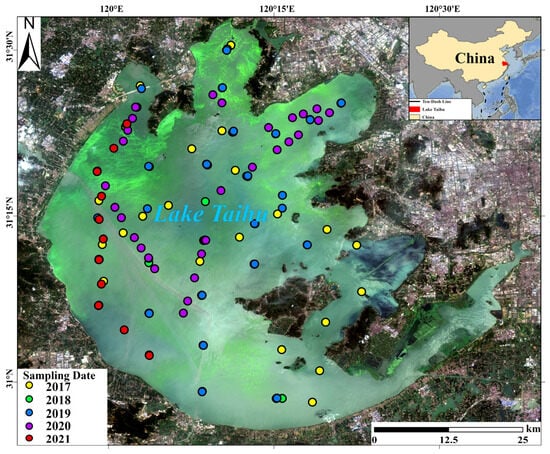
Figure 1.
Map of the study area and sampling position.
The Taihu Basin is situated in a subtropical monsoon climate zone, with an average annual precipitation of about 1200 mm and a distinct hot and rainy summer season. On average, rainfall occurs on 120–140 days per year []. In addition, adverse observational conditions such as sun glint further exacerbate the missing-data problem in optical remote sensing imagery. Statistics from MODIS imagery from 2003 to 2023 indicate that the average data-missing rate for Lake Taihu reached 64%, corresponding to an annual average of 227 days without valid observations (Figure 2). Spatially, missing rates are lower in the central lake but higher in nearshore zones due to adjacency effects and other disturbances. Temporally, the missing rates during May–July (67.9%, 77%, and 68.3%) were significantly higher than in other seasons (61.5%). Notably, this period coincides with the critical season for cyanobacterial bloom prevention and control. The extensive absence of remote sensing data severely constrains the timely assessment of the spatial distribution of water quality and limits the effectiveness of bloom forecasting and early warning models.
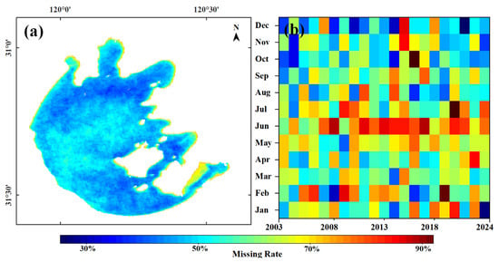
Figure 2.
Missing rate of MODIS images for Lake Taihu (2003–2023): (a) Spatial missing rate, (b) temporal missing rate.
2.2. Data and Preprocessing
2.2.1. In Situ Data
Field sampling data were collected between 2017 and 2021 (Figure 1). Sampling sites were selected following the principle of hydrodynamic zoning of the lake, with a particular focus on bloom-prone areas such as Meiliang Bay and Zhushan Bay. Observations covered three representative seasons: spring (April), summer (July), and autumn (October). At all sites, water samples were consistently collected at a depth of 0.5 m below the surface. During sampling, water was filtered on site using glass fiber filters (pore size: 0.70 μm; diameter: 47 mm; Whatman GF/F). The filters were then immersed in 90% acetone for pigment extraction []. Absorbance of the extracts was measured at 630 nm (A630), 645 nm (A645), 663 nm (A663), and 750 nm (A750) using a UV2600 spectrophotometer. Chl-a concentration was subsequently calculated using Equation (1) [].
where = 11.64, = −2.16, = 0.1, which were determined by the Ministry of Environmental Protection of China based on lake water samples. represents the volume of the extract (10 mL), denotes the volume of filtered lake water (0.05–0.20 L), and is the optical path length of the cuvette (1 cm).
2.2.2. Satellite Remote Sensing Data
In this study, a total of 7865 MODIS Aqua satellite images of Lake Taihu from 2003 to 2023 were collected (https://ladsweb.modaps.eosdis.nasa.gov/, accessed on 24 November 2025). Due to complex aerosol conditions and optically complicated waters, commonly used atmospheric correction algorithms for inland waters, such as NIR–SWIR and MUMM, frequently fail in Lake Taihu [,]. Therefore, an alternative correction scheme was applied. First, Rayleigh scattering and gaseous absorption effects were corrected using the SeaDAS 8.3.0 software in combination with auxiliary meteorological data, yielding Rayleigh-corrected reflectance (Rrc). Second, residual aerosol effects were removed by subtracting the Rayleigh-corrected reflectance at 1240 nm (Rrc(1240)) from the Rayleigh-corrected reflectance in the visible–NIR bands. This procedure significantly increased the number of usable satellite images and has been widely applied in water-color retrieval over turbid waters [,]. This study also downloaded and used several GOCI (Geostationary Ocean Color Imager) quasi-synchronous images for subsequent validation stages. Semi-synchronous GOCI data refer to images acquired within ±1 h of MODIS overpass time, allowing quasi-synchronous temporal matching for cross-sensor validation.
Subsequently, the corrected imagery was preliminarily clipped using the Lake Taihu boundary from the HydroLAKES dataset, and the water body of the lake was extracted with the Normalized Difference Water Index (NDWI). 2-pixel inward buffer was applied during the boundary clipping process to minimize mixed-pixel contamination from adjacent land and shallow shoreline areas. Finally, following Li et al. (2016) [] and Qi et al. (2014) [], pixels with Rrc(1240) > 0.1 or Rrc(555) > 0.25 were identified as clouds and removed from the original imagery.
2.2.3. Retrieval of Chl-a
The Chl-a concentration of Lake Taihu was retrieved using the estimation algorithm proposed by Shi et al. (2017) [].
where Rrc (645) and Rrc (859) are atmospherically Rayleigh-corrected MODIS-Aqua data at 645 nm and 859 nm, respectively. Its retrieval accuracy was validated against 76 independent in situ Chl-a measurements collected in Lake Taihu for this study. The results showed a root mean square error (RMSE) of 7.52 μg/L and a correlation coefficient (R) of 0.86 (Figure S1), indicating that the algorithm achieves high accuracy in Lake Taihu and can be further applied to generate a long-term Chl-a concentration dataset.
3. Spatiotemporal Seamless Reconstruction Algorithm
Four interpolation methods—Kriging Interpolation, SG Filtering, DINEOF, and DINCAE—were applied to reconstruct the original dataset. The performance and effectiveness of these reconstruction methods were comprehensively evaluated using three validation approaches: in situ measurements, semi-synchronous GOCI data, and artificially generated cloud masks. The optimal algorithm was then selected for further application (Figure 3).
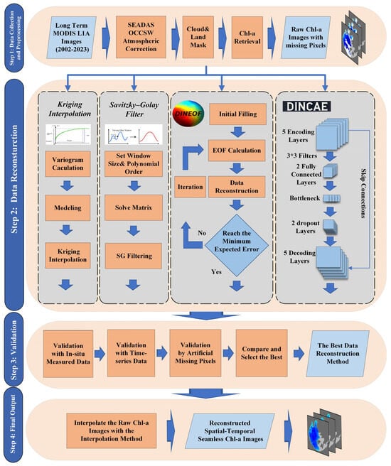
Figure 3.
Working flow of data spatiotemporal–seamless reconstruction.
3.1. Introduction to the Algorithms
3.1.1. Kriging Interpolation
Kriging Interpolation is a classical spatial interpolation method that predicts missing data based on the spatial autocorrelation of observations. Its core concept lies in determining the weights of interpolation points by minimizing interpolation error, thereby estimating the values at missing locations []. First, the method calculates the variogram between known data points to characterize their spatial dependence:
where is the semivariance at lag distance , is the observed value, and is the number of pairs at separation .
Secondly, the missing value at location is then estimated as a weighted linear combination of neighboring observations:
where the weights are determined to minimize estimation variance under the unbiasedness constraint .
The Kriging interpolation parameters are defined as follows: the nugget effect is set to 0.1, representing the contribution of small-scale variability; the range is set to 50, which determines the distance over which spatial correlation is considered significant; and the sill is set to 1, indicating the asymptotic value of the variance at large distances.
A major advantage of Kriging interpolation is that it provides an error estimate for each interpolated point, enabling relatively high accuracy even under conditions of uneven spatial distribution []. This method is particularly suitable for scenarios with strong spatial autocorrelation and is effective in reconstructing data with spatially dependent features, such as water quality parameters [].
3.1.2. Savitzky–Golay Filtering
SG Filtering is a time-series interpolation method based on polynomial smoothing, commonly applied to handle noisy or incomplete temporal datasets []. In SG Filtering, data within a moving window are locally fitted with a polynomial, enabling both smoothing and gap filling. Specifically, an appropriate window size is selected, and polynomial regression is performed within that window to generate a smoothed data curve:
where denotes the signal within the window, in this study, the size of the window is set as 7, and are polynomial coefficients estimated by means of least squares. represents the variable, and denotes the exponent indicating the number of times is multiplied by itself. The smoothed (or interpolated) value at the center of the window, , can then be expressed as a weighted linear combination of the input values:
where are the convolution coefficients derived from the polynomial fitting.
This method effectively removes high-frequency noise while preserving the overall trend of the time series []. For lake water quality data with strong periodicity or long-term trends, SG Filtering can retain spatiotemporal variation characteristics and fill missing values through localized fitting, making it well suited for the restoration of time-series data [].
3.1.3. DINEOF
DINEOF is a spatiotemporal interpolation algorithm that adaptively captures the structure of data without requiring prior statistical information, making it particularly suitable for large-scale and complex spatiotemporal datasets []. Its main advantage lies in its ability to effectively fill missing values across multiple spatial and temporal scales, thereby providing accurate reconstruction results even under high missing rate conditions []. DINEOF is based on Empirical Orthogonal Function (EOF) decomposition []. The core idea is to extract the dominant spatiotemporal modes of variability through EOF decomposition and then use these modes to iteratively reconstruct the missing data. The main parameter settings of the DINEOF algorithm in this study were determined by trial and error (Table 1).

Table 1.
The parameter settings of the DINEOF algorithm.
The main implementation steps include:
- (1)
- Construction of the Initial Data Matrix:
Let the observation data be represented by a matrix , where each row corresponds to a different time point and each column corresponds to a spatial location. Assume , where is the number of time points and is the number of spatial positions. The data matrix contains missing values, with denoting the entry at the row and column; if the value is missing, it is recorded as :
- (2)
- Initial Filling:
Before performing EOF decomposition, the DINEOF algorithm first applies a simple imputation method (e.g., mean filling or nearest-neighbor filling) to replace the missing values, thereby generating a preliminarily filled matrix . This provides an initial complete matrix for subsequent analysis.
- (3)
- EOF Decomposition:
The filled data matrix is decomposed using EOF analysis to obtain the spatial mode matrix and the temporal mode matrix . In other words, the data matrix is decomposed as:
where is the spatial mode matrix, where each column represents a spatial mode, and is the temporal mode matrix, where each row represents a temporal mode. The parameter denotes the number of principal components, which is typically smaller than both and .
- (4)
- Reconstruction of Missing Data:
The missing values are reconstructed using the spatial modes and temporal modes obtained from the EOF decomposition. For a missing observation , its value is estimated by the weighted sum of the corresponding spatial and temporal modes:
where denotes the reconstructed value at the row and column, while and represent the th principal component of the spatial and temporal modes, respectively.
- (5)
- Iterative Optimization:
The reconstructed data are used as new inputs for iterative refinement. In each iteration, EOF decomposition is recalculated based on the currently reconstructed matrix, and the estimates of the missing values are updated accordingly. This process is repeated until convergence is achieved:
where denotes the iteration, and the process continues until the difference between the reconstructed data matrix and that of the previous iteration falls below a predefined threshold.
3.1.4. DINCAE
DINCAE is a deep learning–based spatiotemporal interpolation method that reconstructs missing data by combining convolutional neural networks with autoencoders []. DINCAE first employs convolutional layers to extract spatial features from the data, capturing spatial dependencies in complex environments such as inland and coastal waters []. It then uses an autoencoder to map the data into a low-dimensional latent space, where higher-level spatiotemporal features are learned [,]. The encoded data are subsequently passed through a decoder to restore them to the original space, thereby generating reconstructed values for the missing data. In the execution of the code, the number of epochs is set to 1000, and the batch size is set to 32. Both the encoder and decoder employ the default architecture.
A key advantage of DINCAE lies in its deep learning framework, which can automatically learn spatiotemporal features without the need to manually define specific modes or rules. Moreover, DINCAE demonstrates strong flexibility and accuracy when handling data with complex nonlinear relationships, making it particularly suitable for cases with high proportions of missing data or inherent nonlinear spatiotemporal dependencies []. Through iterative training, DINCAE adaptively adjusts its model parameters, progressively improving reconstruction accuracy. This capability highlights its substantial potential for reconstructing remote sensing imagery and other datasets characterized by complex spatial structures and temporal variability [].
3.2. Evaluation Methods
In this study, both qualitative and quantitative methods were employed to evaluate and analyze the performance of four reconstruction algorithms. Lake algal blooms typically occur when algal cells rapidly rise and accumulate under favorable hydrological and climatic conditions. The unpredictable and sudden nature of these blooms increases the complexity of Chl-a variability, making data reconstruction more challenging. Therefore, it is crucial to assess the algorithms’ performance in both bloom and non-bloom scenarios. Given that algal blooms are more frequent during the summer, leading to greater variability in Chl-a concentrations, and that cloud cover and rainfall often result in significant data loss in satellite imagery, the study divided the reconstruction scenarios into bloom and non-bloom conditions. Additionally, to simulate varying levels of data loss, artificial cloud masks were applied to create three scenarios with low, medium, and high cloud cover, allowing for a more thorough evaluation of algorithm performance (Figure 4).
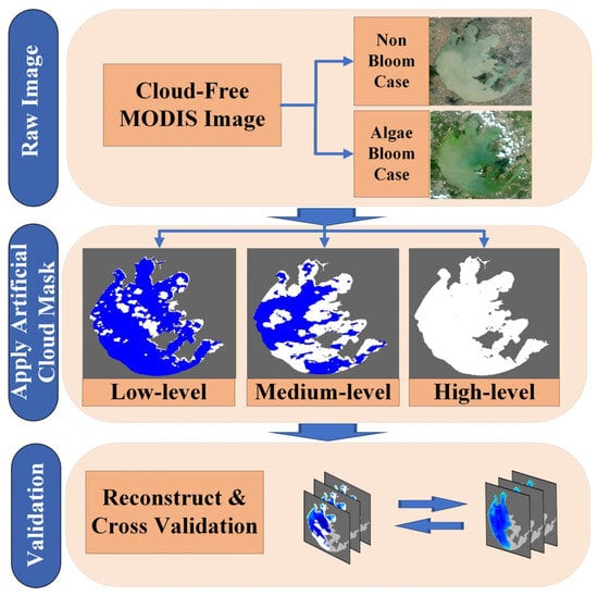
Figure 4.
Working flow of validation through an artificial cloud.
For qualitative evaluation, intuitive visual comparisons of the reconstruction results from the four algorithms were conducted to assess their performance differences across various scenarios. For quantitative evaluation, the root mean square error (RMSE), mean absolute percentage error (MAPE), and correlation coefficient (R) were used as metrics to quantitatively compare the reconstruction performance of the algorithms. These metrics are defined as:
where denotes the observed values, the reconstructed values, and N the total number of samples. . and represent the mean of observed and reconstructed values, respectively.
4. Result
4.1. Spatial Pattern Comparison
To comprehensively assess the gap-filling performance of different algorithms under various conditions, two representative scenarios: “bloom” and “non-bloom” were selected to illustrate their reconstruction effectiveness and applicability across different missing-data patterns (Figure 5 and Figure 6).
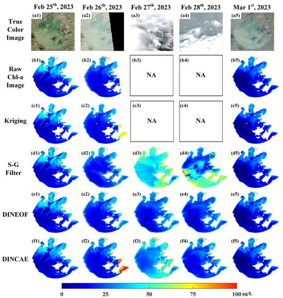
Figure 5.
Comparison of reconstructed Chl-a concentration results from different methods under the no-algal-bloom scenario: (a1–a5) true color image from MODIS; (b1–b5) raw Chl-a concentration image from MODIS; (c1–c5) reconstructed Chl-a concentration using Kriging Interpolation; (d1–d5) reconstructed Chl-a concentration using SG Filtering; (e1–e5) reconstructed Chl-a a concentration using DINEOF; (f1–f5) reconstructed Chl-a concentration using DINCAE.
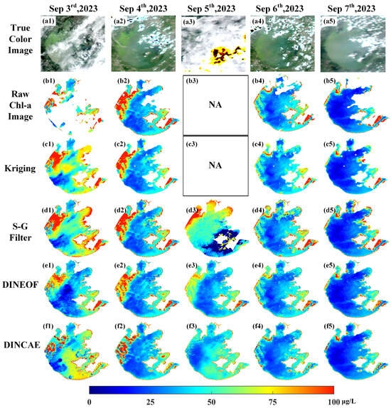
Figure 6.
Comparison of reconstructed Chl-a concentration results from different methods under the algal bloom scenario: (a1–a5) true-color image from MODIS; (b1–b5) raw Chl-a concentration image from MODIS; (c1–c5) reconstructed Chl-a concentration using Kriging Interpolation; (d1–d5) reconstructed Chl-a concentration using SG Filtering; (e1–e5) reconstructed Chl-a concentration using DINEOF; (f1–f5) reconstructed Chl-a concentration using DINCAE.
In the no-algal-bloom scenario, Chl-a concentrations were relatively homogeneous, with limited spatiotemporal variability (Figure 5). Taking 25 February–1 March 2023, as an example, the Kriging interpolation algorithm demonstrated clear limitations when dealing with completely missing datasets (Figure 5(c3,c4)). The SG Filtering method performed reasonably well under conditions of small-scale data gaps (Figure 5(d2)), but produced distortions when the missing rate was high (Figure 5(d3,d4)). By contrast, both DINEOF and DINCAE exhibited superior performance in non-bloom conditions, where their reconstructed outputs maintained good spatial continuity and closely matched the distribution patterns of non-missing regions (Figure 5e,f). DINCAE-reconstructed data exhibited greater spatiotemporal intensity and variability compared with DINEOF results.
In the algal-bloom scenario, Chl-a concentrations exhibited strong spatiotemporal variability, posing greater challenges for reconstruction (Figure 6). Taking 3–7 September 2023, as an example, Kriging Interpolation was able to partially restore local features when missing rates were low, but its performance rapidly deteriorated as the extent of missing data increased, nearly failing under conditions of high or complete data loss (Figure 6(c3,c4)). SG Filtering performed slightly better than Kriging in some areas (Figure 6(d3)), yet still suffered from over-smoothing and loss of detail. In contrast, DINEOF and DINCAE maintained strong performance under bloom conditions, effectively reconstructing the spatial distribution of Chl-a concentrations. Their results largely captured the occurrence and expansion dynamics of blooms (Figure 6(e3,f3)). Nevertheless, it should be noted that DINCAE tended to overestimate Chl-a values in certain local areas (Figure 6(f1,f2)).
4.2. Validation with Quasi-Synchronous GOCI Imagery
In this study, the reconstruction results were evaluated by comparing them with quasi-synchronous, cloud-free GOCI imagery acquired on the same day (Figure 7). Considering the differences between the MODIS and GOCI sensors, the comparison primarily focused on the spatial distribution differences between MODIS-reconstructed Chl-a concentrations and the GOCI-derived Chl-a proxy index . The results showed that the reconstructed MODIS Chl-a concentrations were generally consistent with the GOCI retrievals in terms of overall spatial patterns and trends, indicating that the reconstruction algorithms were able to effectively restore the spatial distribution characteristics and variation dynamics of Chl-a.
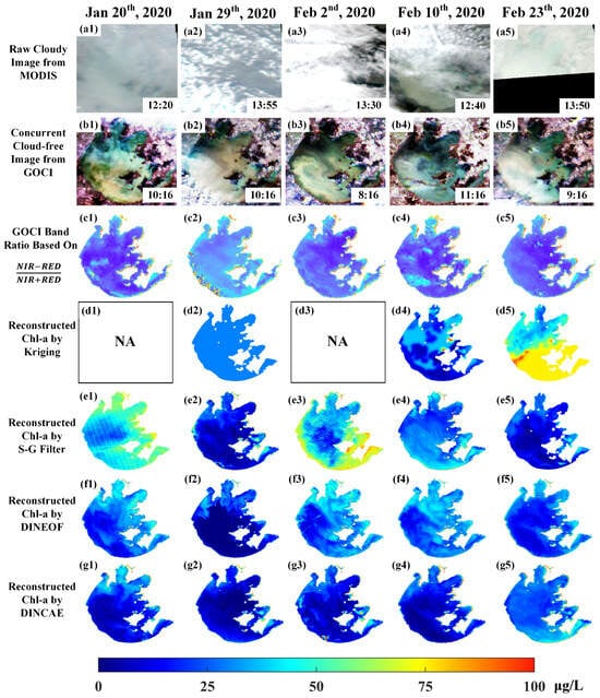
Figure 7.
Comparison of reconstructed MODIS images with quasi-synchronous cloud-free GOCI images: (a1–a5) raw cloudy image from MODIS, (b1–b5) semi-synchronous cloud-free image from GOCI, (c1–c5) GOCI band ratio image based on NIR-RED/NIR+RED, (d1–g5) reconstructed Chl-a concentration by different interpolation methods.
It should be noted, however, that due to the difference in overpass times between the two satellites—MODIS Aqua typically acquiring data in the afternoon local time and GOCI making cloud-free observations mostly in the morning on the same day—certain discrepancies were observed. For example, on 20 January 2020, GOCI detected a bloom event in the southwestern part of the lake, while the reconstructed MODIS results failed to capture this phenomenon (Figure 7a).
4.3. Validation with In Situ Measurements
To further quantitatively validate the accuracy of the reconstruction algorithms, cloud-affected remote sensing imagery was compared with synchronous in situ sampling data (Figure 8). The results demonstrated that both DINEOF and DINCAE achieved the highest reconstruction accuracy, yielding the strongest correlations (R = 0.77 and 0.79) and the lowest errors (RMSE = 14.38 and 17.12 μg/L), highlighting their superiority in recovering missing data. In contrast, the Kriging interpolation and SG Filtering methods exhibited relatively lower accuracy (R = 0.61, RMSE = 23.11 μg/L; R = 0.70, RMSE = 17.93 μg/L).
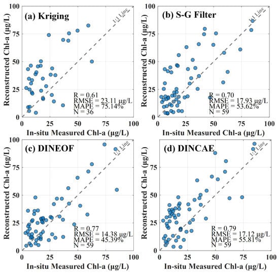
Figure 8.
Validation of reconstructed Chl-a data based on concurrent in situ data shown in Figure 1: (a) Kriging Interpolation; (b) SG Filtering; (c) DINEOF; (d) DINCAE.
We further selected several representative case dates in which satellite imagery was severely affected by cloud cover, thereby providing an effective means to evaluate the performance of different reconstruction algorithms under conditions of missing data (Figure 9). The case study results were largely consistent with the overall findings. Kriging interpolation could not be applied in scenarios with completely missing data (Figure 9(a2,b2)) and yielded the lowest correlation (R = 0.60; Figure 9(c2)). The SG Filtering method performed reasonably well on 26 April 2018 (Figure 9(a3)), but its reconstruction accuracy declined significantly under high missing rates (Figure 9(b3)). Moreover, even under low missing rates, its performance was inferior to that of DINEOF and DINCAE (Figure 9(c3)). DINEOF and DINCAE exhibited comparable performance overall. For 26 April 2018, DINCAE achieved better results (R = 0.76; Figure 9(a4,a5)). In contrast, for 28 December 2019, DINEOF performed better (R = 0.69; Figure 9(b4,b5)). For 30 October 2020, the two methods achieved similar accuracies (R = 0.88, RMSE = 12.18 μg/L for DINEOF; R = 0.85, RMSE = 15.02 μg/L for DINCAE; Figure 9(c4,c5)).
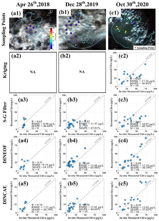
Figure 9.
Examples of validation of reconstructed data based on concurrent in-situ data: (a1–c1) Map of the sampling points;(a2–c2) Kriging Interpolation; (a3–c3) SG Filtering; (a4–c4) DINEOF; (a5–c5) DINCAE.
4.4. Validation Under Artificial Cloud Scenarios
In this study, artificial cloud masks were used to simulate different missing-data scenarios in order to evaluate the performance of the reconstruction algorithms. Still, two types of conditions were considered—bloom and non-bloom—combined with three levels of missing rates (low, medium, and high; Figure 10 and Figure 11).
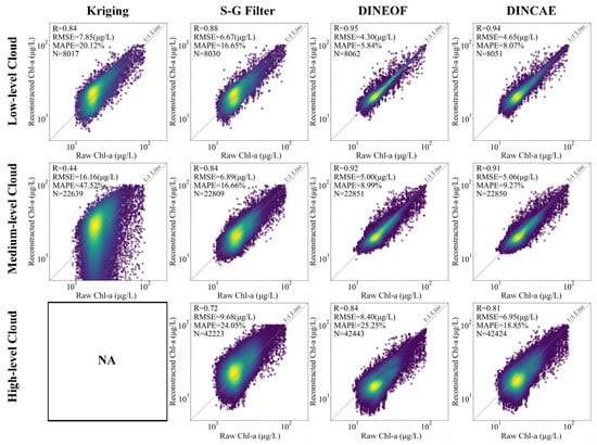
Figure 10.
Scatter density plots of reconstructed Chl-a concentration based on different methods and raw MODIS-derived Chl-a data under different artificial cloud scenarios in the absence of algal bloom.
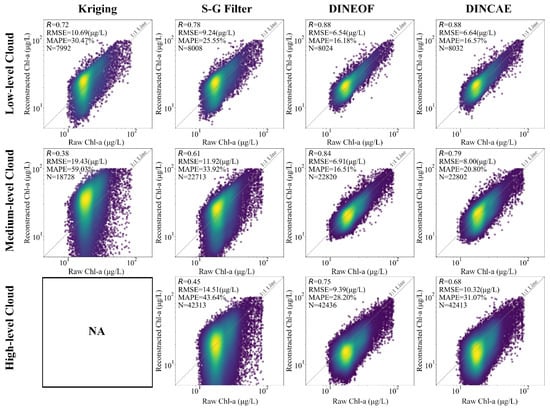
Figure 11.
Scatter density plots of reconstructed Chl-a concentration based on different methods and raw MODIS-derived Chl-a concentration data under different artificial cloud scenarios in the presence of an algal bloom.
In the no-algal-bloom scenarios (Figure 10), the Kriging interpolation algorithm achieved relatively high reconstruction accuracy under low missing rates (R = 0.84, RMSE = 7.85 μg/L). However, as the missing proportion increased, its performance declined sharply (R = 0.44, RMSE = 16.16 μg/L) and eventually failed under high-level cloud masking. Similarly, the reconstruction accuracy of the SG Filtering method also deteriorated rapidly as the missing rate increased (R = 0.88, 0.84, and 0.72 for low, medium, and high missing levels, respectively), indicating its limited capacity to handle high missing-rate scenarios.
By contrast, both DINEOF and DINCAE demonstrated robust performance under low and medium missing conditions. Remarkably, even under extreme situations where the original data were completely missing, the two algorithms maintained relatively high reconstruction accuracy. DINEOF achieved higher correlation coefficients, while DINCAE yielded lower RMSE values (DINEOF: R = 0.84, RMSE = 8.40 μg/L; DINCAE: R = 0.81, RMSE = 6.95 μg/L).
In the algal-bloom scenarios (Figure 11), the performance of all algorithms declined compared with the no-algal-bloom cases, particularly under high missing-rate conditions. The most pronounced decrease was observed for the SG Filtering method, where reconstruction accuracy dropped sharply, with the correlation coefficient falling from R = 0.72 in the non-bloom scenario to R = 0.45 in the bloom scenario. Scatter density plots further revealed that the reduction in accuracy for DINEOF and DINCAE under high missing rates was primarily caused by widespread underestimation across numerous data points. This indicates that although these algorithms were able to partially recover the missing data, they failed to accurately capture the spatial distribution of bloom areas. As bloom events are highly stochastic phenomena with considerable uncertainty in their extent and location, they pose stricter challenges to the performance of reconstruction algorithms.
5. Discussion
5.1. Advantages and Limitations of the Algorithms
The differences in the performance of various algorithms for missing-data reconstruction are essentially determined by their respective approaches to utilizing spatiotemporal information and the assumptions underlying their models.
Kriging interpolation is grounded in the principle of spatial autocorrelation. By quantifying spatial dependence through variograms and minimizing estimation variance, it achieves unbiased optimal estimates under conditions of strong spatial continuity and limited missing regions. Its advantages lie in its strong theoretical interpretability and computational simplicity. However, when spatial variability is pronounced or the missing region is extensive, spatial information alone is insufficient to support reliable estimation []. This often results in over-smoothing, with poor capability to capture local abrupt phenomena such as cyanobacterial bloom outbreaks [].
The SG Filtering is based on local polynomial fitting and relies on the assumption of temporal continuity. It is suitable for denoising and smoothing time series under low missing rates and stable background conditions, effectively preserving trends while suppressing noise []. Nonetheless, its limitations arise from the absence of spatial information. When heterogeneous temporal trends exist across different regions, they cannot be captured. Moreover, under non-stationary or abrupt changes, polynomial fitting may misinterpret valid dynamics as noise and over-smooth them, especially when consecutive data gaps undermine its mathematical foundation [].
DINEOF reconstructs missing values iteratively through Empirical Orthogonal Function (EOF) decomposition, extracting dominant spatiotemporal modes under the assumption that a limited number of modes explain most of the variance []. A key advantage of DINEOF is that it does not require prior statistical assumptions and simultaneously leverages both spatial and temporal information, making it robust even under conditions of extensive data gaps. In particular, it performs well in capturing large-scale coherent variability and provides stable reconstructions in datasets with moderate to high missing rates. However, its reliance on linear dimensionality reduction means that it has limited capacity to represent complex nonlinear spatiotemporal dynamics. Furthermore, DINEOF can be sensitive to noise and outliers; disturbances in the leading modes may propagate through the iterative reconstruction, thereby reducing accuracy [,].
DINCAE leverages the end-to-end learning capacity of convolutional autoencoders to automatically extract nonlinear spatiotemporal features, making it well suited to complex and abrupt events such as algal bloom outbreaks. The local perception and weight-sharing mechanisms of convolution allow it to capture global patterns while recovering local anomalies. Its limitations, however, include a strong dependence on large-scale, high-quality training datasets and substantial computational resources []. In cases of limited samples, the model is prone to overfitting, and its “black-box” nature results in relatively poor interpretability [,].
Overall, Kriging and SG Filtering represent purely spatial and purely temporal linear interpolation methods, whose applicability depends largely on the regularity of missing-data patterns and the stability of the background. In contrast, DINEOF and DINCAE integrate spatiotemporal information and are better suited to addressing large-scale gaps and complex dynamics, maintaining robustness even under extensive data loss. In this study, we assess the applicability and performance of multiple reconstruction algorithms on remote sensing imagery of representative cloudy and rainy lakes in the middle and lower reaches of the Yangtze River, China. Nevertheless, given the complexity and heterogeneity of inland water bodies—such as high-altitude lakes and saline lakes—the generalizability and effectiveness of these algorithms require further systematic investigation.
5.2. Future Perspectives
Existing methods for missing-data reconstruction have demonstrated good performance under routine conditions; however, their stability and accuracy remain inadequate when confronted with highly complex missing patterns and abrupt events such as algal bloom outbreaks. The underlying challenge lies in their limited capacity to capture local features and nonlinear dynamics, often leading to over-smoothing or localized overestimation. One critical challenge is the computational efficiency of the algorithm and its demand for computational resources. With the rapid increase in the volume of water quality monitoring data, particularly with the use of multi-source data fusion and high-resolution remote sensing data, effectively processing and analyzing this massive amount of data has become a significant challenge. Machine learning-based reconstruction algorithms, such as DINCAE, often rely on substantial computational resources, such as high-performance processors and large amounts of memory, which can lead to computational bottlenecks in real-time or large-scale monitoring applications. Another critical challenge for future algorithm optimization is the accurate recovery of local details. Most existing methods prioritize restoring overall trends but lack sensitivity at finer scales, making it difficult to capture subtle spatial heterogeneity associated with bloom processes. Future efforts could focus on introducing multi-scale feature extraction mechanisms into models or combining multi-source high-resolution remote sensing data, thereby strengthening the ability to resolve local abrupt features and achieving breakthroughs in detail reconstruction [,,].
Future research can advance improvements from both observational-system and algorithm-optimization perspectives, thereby providing stronger data support for eutrophication management, bloom early warning, and ecological protection.
From the perspective of observational systems, it is essential to accelerate the establishment of an integrated “Satellite–Airborne–Ground” monitoring framework. Satellite remote sensing provides large-scale and long-term coverage; UAVs and airborne sensors can bridge the spatiotemporal gaps of satellite observations; and ground-based automatic monitoring stations, shore-based remote sensing, and video surveillance can deliver high-frequency, fine-resolution water quality data []. The complementary integration of these platforms would not only supply valuable prior information and validation support for reconstruction algorithms but also significantly enhance the continuity and accuracy of lake water environment monitoring [].
From the perspective of algorithm optimization, one direction is to further explore mechanisms for multi-source data fusion. Integrating water quality information from multiple-source observations can provide high-frequency, localized supplementary inputs, thereby improving the robustness of reconstruction results []. Moreover, highly variable processes such as algal blooms are often driven by meteorological and hydrodynamic conditions. Incorporating auxiliary variables such as temperature, wind speed, hydrodynamics, and nutrient concentrations into reconstruction models can help overcome the inherent limitations of relying solely on satellite imagery and enhance model adaptability to complex dynamic scenarios []. Another direction for algorithm optimization is the deep integration of AI techniques with mechanistic models. Mechanistic models offer advantages such as clear underlying principles, rigorous logical structure, and strong interpretability, providing reliable theoretical support for understanding system behavior []. In contrast, machine learning excels at automatic feature extraction, adapting to complex nonlinear relationships, and discovering latent patterns in large-scale datasets. Combining the two allows models to achieve higher accuracy and better generalization while maintaining interpretability and physical consistency []. Consequently, this direction is likely to become a major research hotspot in future algorithm development.
The application of data reconstruction technology in water quality monitoring, especially in monitoring and early warning systems for complex water quality events, holds significant potential. As the demand for water quality monitoring continues to increase, particularly in ecologically sensitive areas such as lakes, rivers, and reservoirs, the accurate reconstruction of missing data becomes crucial for ensuring the efficient operation of monitoring systems. In conclusion, the potential of data reconstruction technology in water quality monitoring is not limited to filling in missing data but also facilitates the transition of water quality management systems from passive response to proactive early warning. In the future, with the continuous development of multi-source data fusion technologies and artificial intelligence algorithms, water quality monitoring systems will become more intelligent and precise, bringing greater scientific value and practical significance for environmental protection and addressing changes in water quality [,].
6. Conclusions
This study comprehensively examined the application of multiple interpolation and reconstruction algorithms for reconstructing missing Chl-a data in Lake Taihu, including Kriging Interpolation, SG Filtering, DINEOF, and DINCAE. By evaluating algorithm performance across different scenarios, the results demonstrate that each method has unique advantages and limitations depending on the type and extent of data gaps. Kriging interpolation and SG Filtering perform well under low missing rates, but their effectiveness decreases substantially in cases of large-scale gaps or complex environments, particularly in capturing spatial-temporal heterogeneity in Chl-a concentrations. In contrast, DINEOF and DINCAE exhibit stronger reconstruction capabilities, especially under moderate-to-high missing rates and dynamic bloom conditions, where they can more accurately reconstruct the spatiotemporal distribution of Chl-a, highlighting the potential of deep learning methods in complex ecological environments.
This study also reveals the potential of reconstruction algorithms in addressing sudden water quality events, such as algal blooms. Data reconstruction methods not only fill in missing data but also more accurately reconstruct the spatiotemporal distribution of water quality, providing important decision-making support. The results underscore the potential of these advanced techniques in maintaining the reliability and continuity of long-term monitoring, especially in challenging conditions. This study illustrates the reliability of statistical and deep learning methods in the reconstruction of lake water color data, providing valuable insights for improving ecological management and supporting decision-making in the sustainable monitoring of water bodies.
Supplementary Materials
The following supporting information can be downloaded at https://www.mdpi.com/article/10.3390/rs17233843/s1.
Author Contributions
Conceptualization, M.S.; Data curation, Y.S.; Formal analysis, Y.S.; Writing—original draft, Y.S.; Writing—review and editing, Y.S., Z.C., Z.Q., C.Y., H.D., H.Y. and M.S. All authors have read and agreed to the published version of the manuscript.
Funding
This work was supported by the National Natural Science Foundation of China [42201403, 42425104], the Natural Science Foundation of Jiangsu Province [BK20221159], and the Science and Technology Planning Project of NIGLAS [NIGLAS2022TJ17, NKL2023-ZD01].
Data Availability Statement
The data presented in this study are available upon request from the corresponding author.
Acknowledgments
The authors express sincere gratitude to all the teachers and classmates who provided guidance and suggestions for this research. Special thanks are extended for the use of the following algorithms and tools in this study: DINEOF (https://github.com/aida-alvera/DINEOF, accessed on 24 November 2025), DINCAE (https://github.com/gher-uliege/DINCAE.jl, accessed on 24 November 2025).
Conflicts of Interest
The authors declare no conflicts of interest.
Abbreviations
The following abbreviations are used in this manuscript:
| Chl-a | Chlorophyll-a |
| SG Filtering | Savitzky–Golay Filtering |
| DINEOF | Data Interpolating Empirical Orthogonal Functions |
| DINCAE | Data Interpolating Convolutional Auto Encoder |
| MODIS | Moderate-resolution Imaging Spectroradiometer |
| GOCI | Geostationary Ocean Color Imager |
References
- Seegers, B.N.; Werdell, P.J.; Vandermeulen, R.A.; Salls, W.; Stumpf, R.P.; Schaeffer, B.A.; Owens, T.J.; Bailey, S.W.; Scott, J.P.; Loftin, K.A. Satellites for long-term monitoring of inland U.S. lakes: The MERIS time series and application for chlorophyll-a. Remote Sens. Environ. 2021, 266, 112685. [Google Scholar] [CrossRef]
- Shen, M.; Cao, Z.; Xie, L.; Zhao, Y.; Qi, T.; Song, K.; Lyu, L.; Wang, D.; Ma, J.; Duan, H. Microcystins risk assessment in lakes from space: Implications for SDG 6.1 evaluation. Water Res. 2023, 245, 120648. [Google Scholar] [CrossRef]
- Luo, J.; Duan, H.; Xu, Y.; Shen, M.; Zhang, Y.; Xiao, Q.; Ni, G.; Wang, K.; Xin, Y.; Qi, T.; et al. Global trends and regime state shifts of lacustrine aquatic vegetation. Innov. 2025, 6, 100784. [Google Scholar] [CrossRef]
- Woolway, R.I.; Kraemer, B.M.; Lenters, J.D.; Merchant, C.J.; O’Reilly, C.M.; Sharma, S. Global lake responses to climate change. Nat. Rev. Earth Environ. 2020, 1, 388–403. [Google Scholar] [CrossRef]
- Xu, X. Environmental Quality Assessment of Tibet Based on 3S. In Progress in Environmental Protection and Processing of Resource, Pts 1-4; Tang, X., Zhong, W., Zhuang, D., Li, C., Liu, Y., Eds.; Applied Mechanics and Materials; Trans Tech Publications Ltd.: Stafa-Zurich, Switzerland, 2013; Volume 295–298, pp. 692–695. [Google Scholar]
- Cao, Z.; Ma, R.; Duan, H.; Pahlevan, N.; Melack, J.; Shen, M.; Xue, K. A machine learning approach to estimate chlorophyll-a from Landsat-8 measurements in inland lakes. Remote Sens. Environ. 2020, 248, 111974. [Google Scholar] [CrossRef]
- Shen, M.; Cao, Z.; Xue, K.; Liu, D.; Qi, T.; Ma, J.; Duan, H. Natural and human activities driving the spatiotemporal variability of water clarity in lakes across Eastern China. Int. J. Appl. Earth Obs. Geoinf. 2022, 114, 103037. [Google Scholar] [CrossRef]
- Cao, Z.; Wang, M.; Ma, R.; Duan, H.; Jiang, L.; Shen, M.; Xue, K.; Su, F. Seamless observations of chlorophyll-a from OLCI and VIIRS measurements in inland lakes. Water Res. 2024, 270, 122825. [Google Scholar] [CrossRef]
- Chen, P.; Wang, B.; Wu, Y.; Wang, Q.; Huang, Z.; Wang, C. Urban river water quality monitoring based on self-optimizing machine learning method using multi-source remote sensing data. Ecol. Indic. 2023, 146, 109750. [Google Scholar] [CrossRef]
- Yuan, L.L.; Jones, J.R. Rethinking phosphorus–chlorophyll relationships in lakes. Limnol. Oceanogr. 2020, 65, 1847–1857. [Google Scholar] [CrossRef]
- Li, L.; Knapp, J.L.; Lintern, A.; Ng, G.-H.C.; Perdrial, J.; Sullivan, P.L.; Zhi, W. River water quality shaped by land–river connectivity in a changing climate. Nat. Clim. Change 2024, 14, 225–237. [Google Scholar] [CrossRef]
- Feng, L.; Wang, X. Quantifying Cloud-Free Observations from Landsat Missions: Implications for Water Environment Analysis. J. Remote Sens. 2024, 4, 0110. [Google Scholar] [CrossRef]
- Zhang, D.D.; Xu, J. Long-Term Monitoring of Surface Water Dynamics and Analysis of Its Driving Mechanism: A Case Study of the Yangtze River Basin. Water 2024, 16, 677. [Google Scholar] [CrossRef]
- Zhang, Y.; Shi, K.; Cao, Z.; Lai, L.; Geng, J.; Yu, K.; Zhan, P.; Liu, Z. Effects of satellite temporal resolutions on the remote derivation of trends in phytoplankton blooms in inland waters. ISPRS J. Photogramm. Remote Sens. 2022, 191, 188–202. [Google Scholar] [CrossRef]
- Cao, Z.; Ma, R.; Duan, H.; Xue, K.; Shen, M. Effect of Satellite Temporal Resolution on Long-Term Suspended Particulate Matter in Inland Lakes. Remote Sens. 2019, 11, 2785. [Google Scholar] [CrossRef]
- Zhang, L.P.; Zhang, L.F.; Du, B. Deep Learning for Remote Sensing Data. IEEE Geosci. Remote Sens. Mag. 2016, 4, 22–40. [Google Scholar] [CrossRef]
- Dunlop, G.R. A Rapid Computational Method for Improvements to Nearest Neighbor Interpolation. Comput. Math. Appl. 1980, 6, 349–353. [Google Scholar] [CrossRef]
- Smith, P.R. Bilinear Interpolation of Digital Images. Ultramicroscopy 1981, 6, 201–204. [Google Scholar] [CrossRef]
- Zimmerman, D.; Pavlik, C.; Ruggles, A.; Armstrong, M.P. An experimental comparison of ordinary and universal kriging and inverse distance weighting. Math. Geol. 1999, 31, 375–390. [Google Scholar] [CrossRef]
- Matheron, G. Kriging or Polynomial Interpolation Procedures—A Contribution to Polemics in Mathematical Geology. Can. Min. Metall. Bull. 1967, 60, 240–244. [Google Scholar]
- Whitlock, C.H.; Kuo, C.Y.; Lecroy, S.R. Criteria for the Use of Regression-Analysis for Remote-Sensing of Sediment and Pollutants. Remote Sens. Environ. 1982, 12, 151–168. [Google Scholar] [CrossRef]
- Sun, R.; Chen, S.H.; Su, H.B.; Mi, C.R.; Jin, N. The Effect of NDVI Time Series Density Derived from Spatiotemporal Fusion of Multisource Remote Sensing Data on Crop Classification Accuracy. ISPRS Int. Geo-Inf. 2019, 8, 502. [Google Scholar] [CrossRef]
- Comina, C.; Foti, S.; Passeri, F.; Socco, L.V. Time-weighted average shear wave velocity profiles from surface wave tests through a wavelength-depth transformation. Soil. Dyn. Earthq. Eng. 2022, 158, 107262. [Google Scholar] [CrossRef]
- Savitzky, A.; Golay, M.J.E. Smoothing + Differentiation of Data by Simplified Least Squares Procedures. Anal. Chem. 1964, 36, 1627–1639. [Google Scholar] [CrossRef]
- Barth, A.; Alvera-Azcárate, A.; Licer, M.; Beckers, J.M. DINCAE 1.0: A convolutional neural network with error estimates to reconstruct sea surface temperature satellite observations. Geosci. Model. Dev. 2020, 13, 1609–1622. [Google Scholar] [CrossRef]
- Alvera-Azcárate, A.; Barth, A.; Beckers, J.M.; Weisberg, R.H. Multivariate reconstruction of missing data in sea surface temperature, chlorophyll, and wind satellite fields. J. Geophys. Res. Ocean. 2007, 112. [Google Scholar] [CrossRef]
- Barth, A.; Alvera-Azcárate, A.; Troupin, C.; Beckers, J.M. DINCAE 2.0: Multivariate convolutional neural network with error estimates to reconstruct sea surface temperature satellite and altimetry observations. Geosci. Model. Dev. 2022, 15, 2183–2196. [Google Scholar] [CrossRef]
- Shen, M.; Duan, H.; Cao, Z.; Xue, K.; Loiselle, S.; Yesou, H. Determination of the downwelling diffuse attenuation coefficient of lake water with the Sentinel-3A OLCI. Remote Sens. 2017, 9, 1246. [Google Scholar] [CrossRef]
- Guo, L. Doing battle with the green monster of Taihu Lake. Science 2007, 317, 1166. [Google Scholar] [CrossRef] [PubMed]
- Qin, B.; Zhu, G.; Gao, G.; Zhang, Y.; Li, W.; Paerl, H.W.; Carmichael, W.W. A Drinking Water Crisis in Lake Taihu, China: Linkage to Climatic Variability and Lake Management. Environ. Manag. 2010, 45, 105–112. [Google Scholar] [CrossRef]
- Duan, H.; Ma, R.; Simis, S.G.H.; Zhang, Y. Validation of MERIS Case-2 water products in Lake Taihu, China. Giscience Remote Sens. 2012, 49, 873–894. [Google Scholar] [CrossRef]
- Duan, H.; Ma, R.; Zhang, Y.; Loiselle, S.A. Are algal blooms occurring later in Lake Taihu? Climate local effects outcompete mitigation prevention. J. Plankton Res. 2014, 36, 866–871. [Google Scholar] [CrossRef]
- Ma, C.; Zhang, H.; Huo, S.; Li, W.; Liu, Y.; Xiao, Z.; Xu, Y.; Wu, F. Improving the Estimation of Nitrogen and Phosphorus Concentrations in Lakes and Reservoirs Using a Stacked Approach. Earth’s Future 2023, 11, e2022EF003013. [Google Scholar] [CrossRef]
- Qin, B.; Paerl, H.W.; Brookes, J.D.; Liu, J.; Jeppesen, E.; Zhu, G.; Zhang, Y.; Xu, H.; Shi, K.; Deng, J. Why Lake Taihu continues to be plagued with cyanobacterial blooms through 10 years (2007–2017) efforts. Sci. Bull. 2019, 64, 354–356. [Google Scholar] [CrossRef] [PubMed]
- Chen, J.; Gao, X.; Xu, X.; Zhu, C.; She, X.; Kong, D.; Xue, K.; Li, Y. Algal Blooms in Lake Taihu: Earlier Onset and Extended Duration. Harmful Algae 2025, 148, 102917. [Google Scholar] [CrossRef]
- Jeffrey, S.T.; Humphrey, G. New spectrophotometric equations for determining chlorophylls a, b, c1 and c2 in higher plants, algae and natural phytoplankton. Biochem. Und Physiol. Der Pflanz. 1975, 167, 191–194. [Google Scholar] [CrossRef]
- Shen, M.; Duan, H.; Cao, Z.; Xue, K.; Qi, T.; Ma, J.; Liu, D.; Song, K.; Huang, C.; Song, X. Sentinel-3 OLCI observations of water clarity in large lakes in eastern China: Implications for SDG 6.3.2 evaluation. Remote Sens. Environ. 2020, 247, 111950. [Google Scholar] [CrossRef]
- Feng, L.; Hou, X.; Li, J.; Zheng, Y. Exploring the potential of Rayleigh-corrected reflectance in coastal and inland water applications: A simple aerosol correction method and its merits. ISPRS J. Photogramm. Remote Sens. 2018, 146, 52–64. [Google Scholar] [CrossRef]
- Cao, Z.; Duan, H.; Feng, L.; Ma, R.; Xue, K. Climate-and human-induced changes in suspended particulate matter over Lake Hongze on short and long timescales. Remote Sens. Environ. 2017, 192, 98–113. [Google Scholar] [CrossRef]
- Li, J.; Wang, S.; Wu, Y.; Zhang, B.; Chen, X.; Zhang, F.; Shen, Q.; Peng, D.; Tian, L. MODIS observations of water color of the largest 10 lakes in China between 2000 and 2012. Int. J. Digit. Earth 2016, 9, 788–805. [Google Scholar] [CrossRef]
- Qi, L.; Hu, C.; Duan, H.; Cannizzaro, J.; Ma, R. A novel MERIS algorithm to derive cyanobacterial phycocyanin pigment concentrations in a eutrophic lake: Theoretical basis and practical considerations. Remote Sens. Environ. 2014, 154, 298–317. [Google Scholar] [CrossRef]
- Shi, K.; Zhang, Y.; Zhou, Y.; Liu, X.; Zhu, G.; Qin, B.; Gao, G. Long-term MODIS observations of cyanobacterial dynamics in Lake Taihu: Responses to nutrient enrichment and meteorological factors. Sci. Rep. 2017, 7, 40326. [Google Scholar] [CrossRef] [PubMed]
- Li, J.; Heap, A.D. A review of comparative studies of spatial interpolation methods in environmental sciences: Performance and impact factors. Ecol. Inform. 2011, 6, 228–241. [Google Scholar] [CrossRef]
- Steffensen, P. Interpolation of precipitation using kriging. In Proceedings of the 13th Conference on Probability and Statistics in the Atmospheric Sciences, San Francisco, CA, USA, 21–23 February 1996; pp. 172–178. [Google Scholar]
- Zheng, Y.L.; Dai, Q.L.; Tu, Z.G.; Wang, L.G. Guided Image Filtering-Based Pan-Sharpening Method: A Case Study of GaoFen-2 Imagery. ISPRS Int. Geo-Inf. 2017, 6, 22. [Google Scholar] [CrossRef]
- Shwetha, H.R.; Kumar, D.N. Estimation of daily vegetation coefficients using MODIS data for clear and cloudy sky conditions. Int. J. Remote Sens. 2018, 39, 3776–3800. [Google Scholar] [CrossRef]
- Povazhnyy, V.; Povazhnyy, A.; Zolotareva, A.; Sgem. Measurements of Chlorophyll-A In Vivo Fluorescence and Water Reflectance by Consumer Digital Cameras for Remote Sensing Data Verification. In Informatics, Geoinformatics and Remote Sensing Conference Proceedings, Sgem 2016; Proceedings of the International Multidisciplinary Scientific GeoConference-SGEM, Albena, Bulgaria, 28 June–7 July 2016; Stef92 Technology Ltd.: Sofia, Bulgaria, 2016; Volume II, pp. 963–970. [Google Scholar]
- Jayaram, C.; Priyadarshi, N.; Pavan Kumar, J.; Udaya Bhaskar, T.V.S.; Raju, D.; Kochuparampil, A.J. Analysis of gap-free chlorophyll-a data from MODIS in Arabian Sea, reconstructed using DINEOF. Int. J. Remote Sens. 2018, 39, 7506–7522. [Google Scholar] [CrossRef]
- Beckers, J.M.; Barth, A.; Alvera-Azcárate, A. DINEOF reconstruction of clouded images including error maps – application to the Sea-Surface Temperature around Corsican Island. Ocean Sci. 2006, 2, 183–199. [Google Scholar] [CrossRef]
- Marchese, C.; Colella, S.; Brando, V.E.; Zoffoli, M.L.; Volpe, G. Towards accurate L4 ocean colour products: Interpolating remote sensing reflectance via DINEOF. Int. J. Appl. Earth Obs. Geoinf. 2024, 135, 104270. [Google Scholar] [CrossRef]
- Li, J.; Sun, W.F.; Zhang, J. Reconstruct Infrared Sea Surface Temperature Data Based on an Improved Dincae Method. In Proceedings of the IGARSS 2023–2023 IEEE International Geoscience and Remote Sensing Symposium, Pasadena, CA, USA, 16–21 July 2023; pp. 4120–4123. [Google Scholar] [CrossRef]
- Barth, A.; Alvera-Azcárate, A.; Troupin, C.; Beckers, J.M.; Van der Zande, D. Reconstruction of Missing Data in Satellite Images of the Southern North Sea Using a Convolutional Neural Network (Dincae). In Proceedings of the 2021 IEEE International Geoscience and Remote Sensing Symposium IGARSS, Brussels, Belgium, 11–16 July 2021; pp. 7493–7496. [Google Scholar] [CrossRef]
- Han, Z.H.; He, Y.J.; Liu, G.Q.; Perrie, W. Application of DINCAE to Reconstruct the Gaps in Chlorophyll-a Satellite Observations in the South China Sea and West Philippine Sea. Remote Sens. 2020, 12, 480. [Google Scholar] [CrossRef]
- Yan, X.T.; Gao, Z.K.; Jiang, Y.T.; He, J.Y.; Yin, J.J.; Wu, J.P. Application of Synthetic DINCAE-BME Spatiotemporal Interpolation Framework to Reconstruct Chlorophyll-a from Satellite Observations in the Arabian Sea. J. Mar. Sci. Eng. 2023, 11, 743. [Google Scholar] [CrossRef]
- Liu, M.; Liu, X.; Liu, D.; Ding, C.; Jiang, J. Multivariable integration method for estimating sea surface salinity in coastal waters from in situ data and remotely sensed data using random forest algorithm. Comput. Geosci. 2015, 75, 44–56. [Google Scholar] [CrossRef]
- Wang, J.H.; Ge, Y.; Heuvelink, G.B.M.; Zhou, C.H. Upscaling In Situ Soil Moisture Observations to Pixel Averages with Spatio-Temporal Geostatistics. Remote Sens. 2015, 7, 11372–11388. [Google Scholar] [CrossRef]
- Wang, C.Z.; Zhang, Z.; Chen, Y.; Tao, F.L.; Zhang, J.; Zhang, W. Comparing different smoothing methods to detect double-cropping rice phenology based on LAI products—A case study in the Hunan province of China. Int. J. Remote Sens. 2018, 39, 6405–6428. [Google Scholar] [CrossRef]
- Ma, C.; Zhao, J.; Ai, B.; Sun, S. Two-Decade Variability of Sea Surface Temperature and Chlorophyll-a in the Northern South China Sea as Revealed by Reconstructed Cloud-Free Satellite Data. IEEE Trans. Geosci. Remote Sens. 2021, 59, 9033–9046. [Google Scholar] [CrossRef]
- Liu, X.; Wang, M. Global daily gap-free ocean color products from multi-satellite measurements. Int. J. Appl. Earth Obs. Geoinf. 2022, 108, 102714. [Google Scholar] [CrossRef]
- Tran, T.T.K.; Bateni, S.M.; Mohebzadeh, H.; Jun, C.; Pandey, M.; Kim, D. Filling gaps in MODIS NDVI data using hybrid multiple imputation-Machine learning and DINCAE techniques: Case study of the State of Hawaii. Adv. Eng. Softw. 2025, 201, 103856. [Google Scholar] [CrossRef]
- Li, Z.K.; Wei, D.M.; Zhang, X.F.; Gao, Y.T.; Zhang, D.J. A Daily High-Resolution Sea Surface Temperature Reconstruction Using an I-DINCAE and DNN Model Based on FY-3C Thermal Infrared Data. Remote Sens. 2024, 16, 1745. [Google Scholar] [CrossRef]
- Liu, H.Z.; Li, Q.Q.; Shi, T.Z.; Hu, S.B.; Wu, G.F.; Zhou, Q.M. Application of Sentinel 2 MSI Images to Retrieve Suspended Particulate Matter Concentrations in Poyang Lake. Remote Sens. 2017, 9, 761. [Google Scholar] [CrossRef]
- Shrestha, S.; Kazama, F. Assessment of surface water quality using multivariate statistical techniques: A case study of the Fuji river basin, Japan. Environ. Model. Softw. 2007, 22, 464–475. [Google Scholar] [CrossRef]
- Xu, J.; Gao, C.; Wang, Y. Extraction of Spatial and Temporal Patterns of Concentrations of Chlorophyll-a and Total Suspended Matter in Poyang Lake Using GF-1 Satellite Data. Remote Sens. 2020, 12, 622. [Google Scholar] [CrossRef]
- Modi, A.; Roxy, M.K.; Ghosh, S. Gap-filling of ocean color over the tropical Indian Ocean using Monte-Carlo method. Sci. Rep. 2022, 12, 18395. [Google Scholar] [CrossRef]
- Duan, H.; Tao, M.; Loiselle, S.; Zhao, W.; Cao, Z.; Ma, R.; Tang, X. MODIS observations of cyanobacterial risks in a eutrophic lake: Implications for long-term safety evaluation in drinking-water source. Water Res. 2017, 122, 455–470. [Google Scholar] [CrossRef] [PubMed]
- Li, J.; Xia, C. Drivers of Spatial and Temporal Dynamics in Water Turbidity of China Yangtze River Basin. Water 2023, 15, 1264. [Google Scholar] [CrossRef]
- Ghezehegn, S.G.; Steef, P.; Hommersom, A.; Nils, D.; Culcea, O.; Krommendijk, B. Hyperspectral remote sensing for estimating coastal water quality: Case study on coast of Black Sea, Romania. In Remote Sensing for Agriculture, Ecosystems, and Hydrology Xvi, Proceedings of the SPIE Remote Sensing, Amsterdam, Netherlands, 22–25 September 2014; Neale, C.M.U., Maltese, A., Eds.; SPIE-International Society Optical Engineering: Bellingham, WA, USA, 2014; Volume 9239. [Google Scholar]
- Leng, L.; Yang, G.D.; Chen, S.B. A Combinatorial Reasoning Mechanism with Topological and Metric Relations for Change Detection in River Planforms: An Application to GlobeLand30’s Water Bodies. ISPRS Int. Geo-Inf. 2017, 6, 23. [Google Scholar] [CrossRef]
- Salah, M.; Salem, S.I.; Utsumi, N.; Higa, H.; Ishizaka, J.; Oki, K. 3LATNet: Attention based deep learning model for global Chlorophyll-a retrieval from GCOM-C satellite. ISPRS J. Photogramm. Remote Sens. 2025, 220, 490–508. [Google Scholar] [CrossRef]
- Guo, Y.; Huang, C.; Zhang, Y.; Li, Y.; Chen, W. A Novel Multitemporal Image-Fusion Algorithm: Method and Application to GOCI and Himawari Images for Inland Water Remote Sensing. IEEE Trans. Geosci. Remote Sens. 2020, 58, 4018–4032. [Google Scholar] [CrossRef]
- Guo, Y.L.; Chen, W.Q.; Feng, X.W.; Zhang, Y.L.; Li, Y.C.; Huang, C.C.; Li, Y. Temporal unmixing-based cloud removal algorithm for optically complex water images. Int. J. Remote Sens. 2021, 42, 4415–4440. [Google Scholar] [CrossRef]
Disclaimer/Publisher’s Note: The statements, opinions and data contained in all publications are solely those of the individual author(s) and contributor(s) and not of MDPI and/or the editor(s). MDPI and/or the editor(s) disclaim responsibility for any injury to people or property resulting from any ideas, methods, instructions or products referred to in the content. |
© 2025 by the authors. Licensee MDPI, Basel, Switzerland. This article is an open access article distributed under the terms and conditions of the Creative Commons Attribution (CC BY) license (https://creativecommons.org/licenses/by/4.0/).