Article

Validation of Soil Temperature Sensing Depth Estimates Using High-Temporal Resolution Data from NEON and SMAP Missions

1
Department of Atmospheric and Oceanic Sciences & Institute of Atmospheric Sciences, Fudan University, Shanghai 200438, China
2
Zhuhai Fudan Innovation Research Institute, Zhuhai 519000, China
3
Shanghai Key Laboratory of Ocean-Land-Atmosphere Boundary Dynamics and Climate Change, Shanghai 200438, China
4
Key Laboratory of Polar Atmosphere-Ocean-Ice System for Weather and Climate, Ministry of Education, Fudan University, Shanghai 200438, China
5
National Ecological Observatory Network (NEON), Battelle, Boulder, CO 80301, USA
*
Author to whom correspondence should be addressed.
Remote Sens. 2025, 17(23), 3845; https://doi.org/10.3390/rs17233845
Submission received: 1 September 2025 / Revised: 18 November 2025 / Accepted: 24 November 2025 / Published: 27 November 2025

Highlights

What are the main findings?
  • The τ-z model accurately estimates soil temperature sensing depth (zTeff), with best performance around 0.2 τ when monotonic conditions are met.
  • Combining SMAP’s soil moisture, the τ-z model achieves high accuracy in estimating zTeff, with RMSD (0.05 m) and unRMSD (0.03 m), and correlations (0.67) between estimated and observed values.
What is the implication of the main findings?
  • The τ-z model proves robust across diverse ecosystems, thereby enhancing confidence in the retrieval of soil moisture and temperature from passive microwave remote sensing.
  • These results provide a solid foundation for advancing applications in agriculture, hydrology, and climate change monitoring.

Abstract

Passive microwave remote sensing of soil moisture is crucial for monitoring the Earth’s water cycle and surface dynamics. The penetration depth during this process is significant, as it influences the accuracy of retrieved soil moisture data. Within L-band remote sensing, tools such as the τ-z model interpret microwave emissions to estimate soil moisture, taking into account the complex interactions between soil and radiation. However, in validating these models against high-temporal-resolution, ground-based measurements, especially from extensive networks like the Terrestrial National Ecological Observatory Network (NEON), further research and validation efforts are needed. This study comprehensively validates the τ-z model’s ability to estimate the soil temperature sensing depth (zTeff) using data from the NEON and Soil Moisture Active Passive (SMAP) satellite missions. A harmonization process was conducted to align the spatial and temporal scales of the two datasets, enabling rigorous validation. We compared soil optical depth (τ)—a parameter capable of theoretically unifying sensing depth representations across wet soil (~0.05 m) to extreme dry/frozen conditions (e.g., up to ~1500 m in ice-equivalent scenarios)—and geometric depth (z) frameworks against outputs from the τ-z model and NEON’s in situ profiles. The results show that: (1) for the profiles that satisfy the monotonic assumption by the τ-z model, zTeff fits the prediction well at about 0.2 τ for the average; (2) Combining SMAP’s soil moisture, the τ-z model achieves high accuracy in estimating zTeff, with RMSD (0.05 m) and unRMSD (0.03 m), and correlations (0.67) between estimated and observed values. The findings are expected to advance remote sensing techniques in various fields, including agriculture, hydrology, and climate change research.

1. Introduction

In recent years, the L-band passive microwave remote sensing technology has garnered considerable scientific attention due to its unparalleled capability in monitoring and retrieving a diverse array of geophysical parameters, notably soil moisture (θ) [1], snow cover [2], and vegetation attributes [3]. This technology leverages the exquisite sensitivity of L-band microwaves to dielectric properties, thereby facilitating the detection of subsurface features that remain elusive to conventional remote sensing methods [4,5].
One of the primary applications of L-band passive microwave remote sensing technology is retrieving θ, as θ profoundly modulates the microwave emission signatures of the Earth’s surface, rendering it an optimal target for L-band sensors. Recent advances in L-band microwave soil moisture retrieval algorithms have aimed to improve the physical consistency and spatial representativeness of the retrieved results. The advent of satellites like SMOS (Soil Moisture and Ocean Salinity) [6] and Soil Moisture Active Passive (SMAP) [7] has revolutionized large-scale θ monitoring. These satellites enable the generation of globally consistent θ products, essential for refining water and energy balance models across diverse geographical regions. Recent developments include incorporating auxiliary factors such as vegetation cover and dynamic extinction coefficients into improved models [8,9], utilizing multi-angular observations [10], synergizing with C- and X-band sensors [11], and coupling physical models with machine learning approaches [12]. These advances have significantly enhanced the accuracy of θ retrievals.
However, they still face challenges in representing the vertical heterogeneity of soil layers and the dynamic sensing depth under varying moisture and vegetation conditions. These challenges underscore the need for physically grounded frameworks to address vertical heterogeneity issues.
Regarding vertical heterogeneity issues, studies have shown that L-band microwaves can penetrate vegetation canopies and the superficial soil layers, enabling the extraction of subsurface soil moisture information. This penetration prowess, coupled with its ability to bypass clouds, underscores the invaluable role of L-band passive microwave remote sensing in monitoring subsurface conditions in environments with complex surface characteristics.
Moreover, the ambiguity associated with the precise penetration depth poses formidable challenges to utilizing L-band satellite products [13,14]. This uncertainty hampers the accurate interpretation of crucial geophysical parameters, such as θ, vegetation biomass, and snow depth, because the exact penetration depth of microwaves at L-band remains unclear. For instance, the sensing depth issue for the L band ranges from wet soil (~0.05 m) [15] to ice sheets (~1500 m) [16]. As a result, the precision and reliability of the derived products are limited.
Several alternative sensing depth models have been proposed for L-band passive microwave soil moisture remote sensing, including empirical depth weighting models [17], theoretical penetration depth models [18], hybrid model-based approaches [19], and machine learning-based methods [20]. Empirical models rely on site-specific calibration and assume homogeneous soil conditions, limiting their generalizability. Theoretical models, although grounded in electromagnetic theory, often oversimplify soil layering and neglect the dynamic effects of vegetation. Hybrid approaches introduce complexity without significant precision gains, and machine learning methods usually lack interpretability and physical grounding, leading to overfitting in specific environments.
In contrast, the τ-z model [21] offers a more physically robust solution by demonstrating the superiority of τ over z and validating it through a forward simulation [15]. The τ-z model incorporates soil thermal properties, depth-dependent attenuation, and explicit vegetation correction through the τ parameter, making it better suited for application across diverse environments. Our objective is to comprehensively validate the τ-z model for estimating soil temperature sensing depth (zTeff) across diverse ecosystems by harmonizing ground-based data with SMAP satellite observations, thereby addressing a critical gap in multi-scale model evaluation under varying environmental conditions. Importantly, this validation will enhance the accuracy of subsurface soil temperature monitoring, a key input for climate models, agricultural water management, and cryospheric studies. By bridging satellite and ground observations, our work advances the operational applicability of L-band remote sensing in global ecological and hydrological research.

2. Materials

SMAP satellite, launched in 2015, provides invaluable brightness temperature (TB) data that offer insight into soil moisture conditions, land surface freeze–thaw states, and other geophysical parameters. These calibrated measurements, captured across L-band channels and with high temporal frequency, are fundamental for deriving θ, monitoring freeze–thaw dynamics, estimating land surface temperatures, and informing climate models. SMAP’s data can be accessed at https://smap.jpl.nasa.gov/data/ (accessed on 1 October 2024).
The Terrestrial National Ecological Observatory Network (NEON) dataset is a rich collection of ecological data spanning the continental United States, including soil temperature (T), moisture (θ), and texture [22]. NEON’s dataset captures T variations at multiple depths, which is essential for understanding ecosystem functions influenced by thermal dynamics. θ, measured through advanced sensors, provides insights into the water content crucial for plant growth, soil stability, and hydrological processes. Soil texture data, determined through laboratory analysis of soil samples, reveal the proportions of sand, silt, and clay particles that influence soil structure, water retention, and nutrient availability. These datasets can be accessed through NEON’s online portal (https://www.neonscience.org/data-collection/soils, provided by Edward Ayres via email on 1 October 2024).
The NEON dataset has been validated against SMAP observations, demonstrating its robust potential for soil moisture retrieval across diverse terrestrial ecosystems, including but not limited to forested regions [23]. The alignment of NEON point measurements with SMAP’s 36 km grid cells follows the methodology outlined in [24], utilizing their pre-processed data. For spatial scaling, NEON site measurements (0–5 cm depth) are aggregated to a 1 km × 1 km grid within a 3 km × 3 km buffer zone around each SMAP pixel center, taking into account geolocation uncertainties. Temporally, NEON data collected at 15 min intervals are matched to SMAP’s 3-day revisit cycle by selecting the median value within ±12 h of SMAP overpass times. The study quantifies uncertainties through RMSD and correlation analysis, achieving RMSD < 0.05 m3/m3 and correlation coefficients > 0.6 in forested areas, with representativeness validated via land cover, soil texture, and topography comparisons [23,25].
In our study, both SMAP and NEON data are identical to those used in [25], allowing for the tracking of data quality control procedures. θ and T values from all layers at 47 sites, spanning from July 2019 to June 2022, are used as ground truth, covering a period of over 36 months. In particular, the site-averaged θ measurements over the 0–10 cm depth interval align with the volume-averaged soil moisture representation used in SMAP calibration/validation protocols [18,19], ensuring consistency with the satellite product’s effective sensing depth. Some sites were excluded from the analysis due to the limited availability of high-quality data. These issues included the ocean’s impact on SMAP measurements (NEON sites GUAN and LAJA in Puerto Rico), insufficient coincidental SMAP and NEON data (BARR, BONA, and HEAL in Alaska), unavailability of NEON soil moisture data (PUUM), and frost heaving, which caused in situ sensor depths to change throughout the time series (TOOL, HEAL, BARR, and BONA in Alaska). As a result, 40 of the 47 NEON terrestrial sites were retained for further analysis [25] to test the τ-z model in various landscapes, including high-biomass landscapes, which are usually excluded in SMAP (Figure 1).
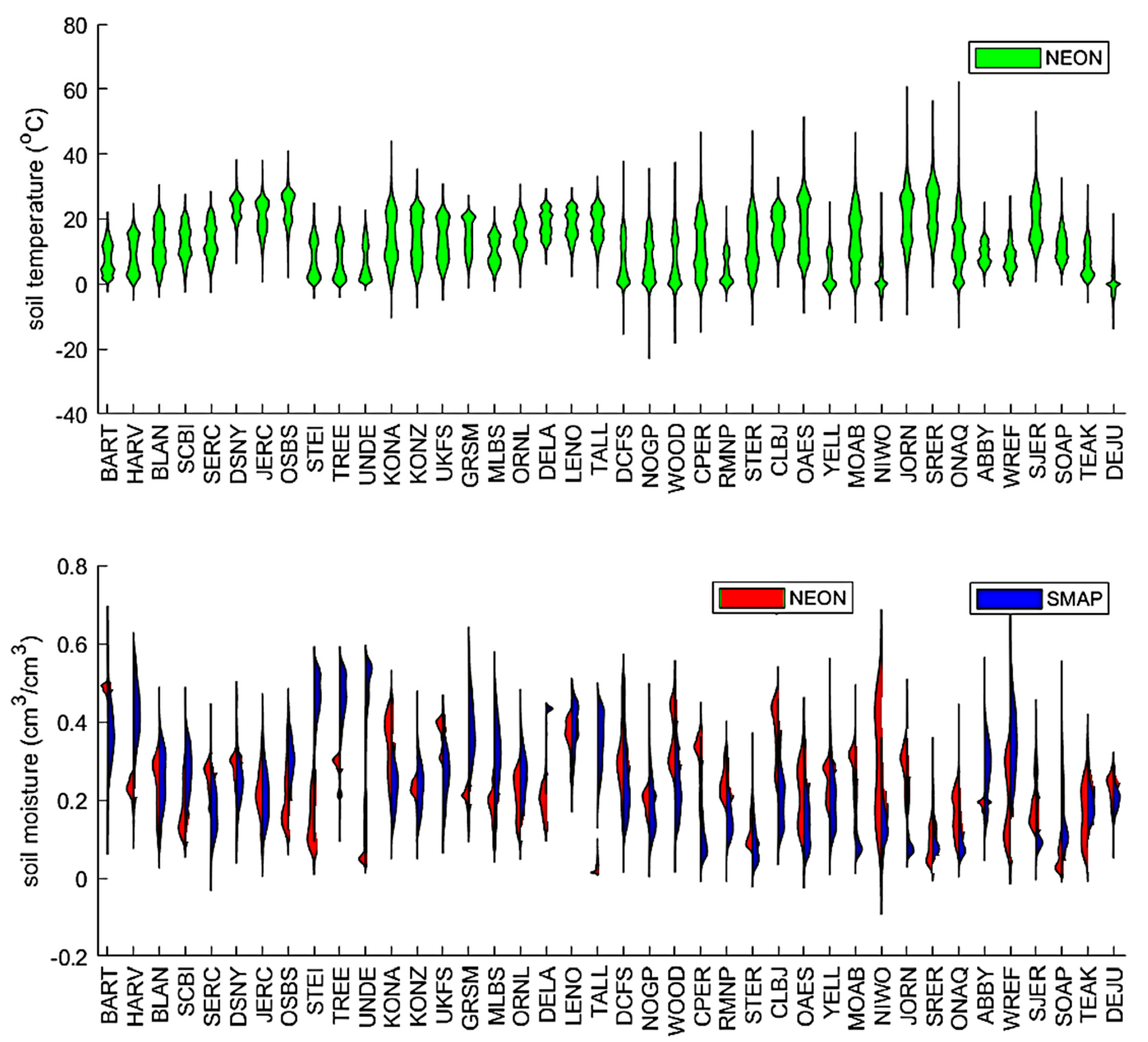
The upper portion of Figure 2 illustrates T ranges across all soil layers at each NEON site, spanning depths from 0.02 m to 2 m (or to a restricting geological feature if shallower), with up to 9 sensor depths per site. The lower portion compares NEON’s site-averaged θ observations (1–11 cm; red) against SMAP’s gridded retrievals (blue). It is essential to note that this comparison represents a sparse network analysis, as NEON sites are spatially discrete. They may not fully capture regional heterogeneity, whereas SMAP provides spatially continuous grid-scale data (36 km resolution).
While NEON’s in situ measurements provide high-precision, localized insights into θ dynamics within specific ecosystems, upscaling these point-based observations to SMAP’s grid scale introduces uncertainties. These include: (1) spatial representativeness gaps between NEON’s localized footprints and SMAP’s pixel-averaged values, and (2) potential mismatches in effective sensing depth (NEON: 1–11 cm vs. SMAP: ~0–10 cm volume-averaged). Despite these challenges, the comparison highlights both the complementary value of ground validation and the need for careful error quantification when integrating sparse network data with satellite products.
In contrast, SMAP’s θ retrieval data provides a global perspective with a lower spatial resolution. While valuable for studying large-scale phenomena, satellite-based estimations are susceptible to atmospheric interference, surface roughness, and vegetation cover, leading to inherent uncertainties. These uncertainties are evident in the smoother trends of the blue line compared to NEON’s more erratic red line. The comparison of the two datasets highlights the complementary nature of NEON’s precise point-based measurements and SMAP’s broader global coverage. NEON’s data offers insights into local-to-regional soil moisture dynamics, while SMAP’s retrievals enable investigations into global-scale processes. The differences between the two datasets highlight the importance of integrating multiple data sources to gain a comprehensive understanding of soil moisture dynamics across various spatial and temporal scales (Figure 2).

3. Methods

Section 3.1 introduces the radiation transfer model, which serves as the foundational framework for simulating how radiation interacts with and propagates through the studied system (e.g., soil or vegetation canopies). To quantify its thermal behavior, Teff, which represents the temperature that best characterizes the system’s radiative energy output, accounts for both surface and subsurface heat exchanges.
For analyzing vertical variations, the τ-z model is then applied to describe how key variables (such as T or θ) change with soil depth in Section 3.2. This model incorporates optical depth (τ) to link measurements at different depths (z), enabling spatial characterization of thermal gradients.
Lastly, to ensure rigorous data analysis, Section 3.3 employs advanced mathematical tools, including statistical indices, which help quantify uncertainties and identify dominant patterns in the datasets.

3.1. Soil Effective Temperature (Teff)

Without considering the impact of soil roughness and vegetation, the primary control function is described by the microwave transfer function as,
T B = ε L T e f f
where TB and Teff are mentioned, εL is the emissivity of the soil bulk determined mainly by θ. Teff effectively reflects the effects of θ and T profiles due to its deeper penetration depth at the L-band. In 1978, Wilheit expressed Teff [26] as
T e f f = 0 T z α z e x p 0 z α z d z d z
where z is the depth from the surface to the soil layer concerned, i.e., the geometric depth. T(z) is the physical temperature at depth z, and α(z) is an attenuation coefficient determined by dielectric constant ε and wavelength λ. ε and ε are the real/imaginary part of ε profiles determined primarily by θ. The detailed form of α(z) is
α z = 4 π λ ε z / 2 ε z 1 2
With Lv’s scheme [21,27], soil optical depth (τ) is derived in Equation (3) as
τ z = 0 z α z d z
So, Teff is rewritten as
T e f f = 0 + T τ e τ d τ
Compared to Equation (2), Equation (5) takes the integral of τ instead of soil depth z. Subsequently, τ is further replaced with t = 1 − e−τ, and Equation (5) evolves to
T e f f = 0 1 T t d t
It is hard to retrieve T from Equation (6) because the equation is not closed, i.e., there are two inputs at least, θ and T on the right side, and only one output (TB) on the left.

3.2. The τ-z Model

Within a comparable τ framework, the τ-z model employs τ, rather than geometric depth (z), to delineate the sensing depth. The factors influencing the microwave-based T-z profile within the soil encompass the soil’s physicochemical characteristics, as well as the frequency and energy of the microwave band. Specifically, physical attributes such as soil density, moisture content, particle size distribution, and particle arrangement have a considerable influence on zTeff.
The τ-z model was proposed in 2019 [21] to quantify the relationship between z and τ, where τ increases with soil depth [17,24]. As a τ value corresponds to only one soil depth for a certain θ and T combination, we can use τ to replace physical soil depth.
T τ = 0 τ T s + a e τ τ   d τ T τ = 0 τ d T s + a e τ τ   d τ
where a is the T gradient in K/τ, Ts is the surface temperature, Td is the soil temperature, which can be considered constant at an annual scale, and τd is the τ corresponding to Td [21]. Then, the τ-z model defines zTeff (i.e., τTeff in terms of τ), which equals Teff. Teff is the soil temperature at zTeff. Furthermore, since the soil depth is between [0,+∞) and τ, we can define t = 1 − eτ ∈ [0,1).
τ T e f f = I n 1 t | T e f f T d T s = 1 ( 1 t ) b · ( l o g ( 1 t ) + 1 )
By knowing τTeff, zTeff is then expressed as
z T e f f = λ τ T e f f ε x 1 2 / 2 π ε x
Since the θ/T profile is not uniform even for a thin layer, Equation (9) works only with a constant θ/T within the depth interval [0, zTeff]. Additionally, we use Teff_nor = T e f f T s T d T s for explanation convenience.

3.3. The Statistics

The validation process is summarized as follows: Starting from a temperature profile (T profile), Teff is derived using Equation (2). Subsequently, by setting Teff equal to the temperature at the effective sensing depth (T|z = zTeff), zTeff is determined. This process allows for the validation of the estimated zTeff obtained from Equations (7)–(9).
To assess the τ-z model’s performance in estimating zTeff, we compared the estimates from the τ-z model with those from NEON’s profiles. We calculated several widely used metrics for analysis and interpretation, including RMSD, unbiased RMSD (unRMSD), mean difference (MD), and Pearson correlation (r). They are defined as
RMSD = 1 N i = 1 N ( x i y i ) 2
where x and y represent the soil temperature sensing depth as estimated by the τ-z model and NEON measurement samples for a given site, i is the individual sample ID, and N is the number of coincidental samples for that site; unRMSD is defined as
unRMSD = 1 N i = 1 N ( x i x ¯ ) ( y i y ¯ ) 2
where x ¯ and y ¯ represent the mean of the soil temperature sensing depth as estimated by the τ-z model and NEON measurements for the site; MD is defined as
MD = 1 N i = 1 N ( x i y i )
and r is defined as
r = i = 1 N ( x i x ¯ ) ( y i y ¯ ) i = 1 N ( x i x ¯ ) 2 i = 1 N ( y i y ¯ ) 2
These metrics address key uncertainty dimensions—error size, relative performance, and pattern consistency—providing a holistic view of model reliability across regions. This approach aligns with our focus on the broad-scale behavior of models. All this information can be found at [24,28,29].

4. Results

The assumptions of the τ-z model for determining soil temperature sensing depth include stratified soil with varying but internally uniform thermophysical properties, the potential for linear or nonlinear temperature variation with depth, the absence of significant internal heat sources or sinks, and a specific mathematical relationship linking zTeff to Teff.

4.1. The τ-z and Its Assumption

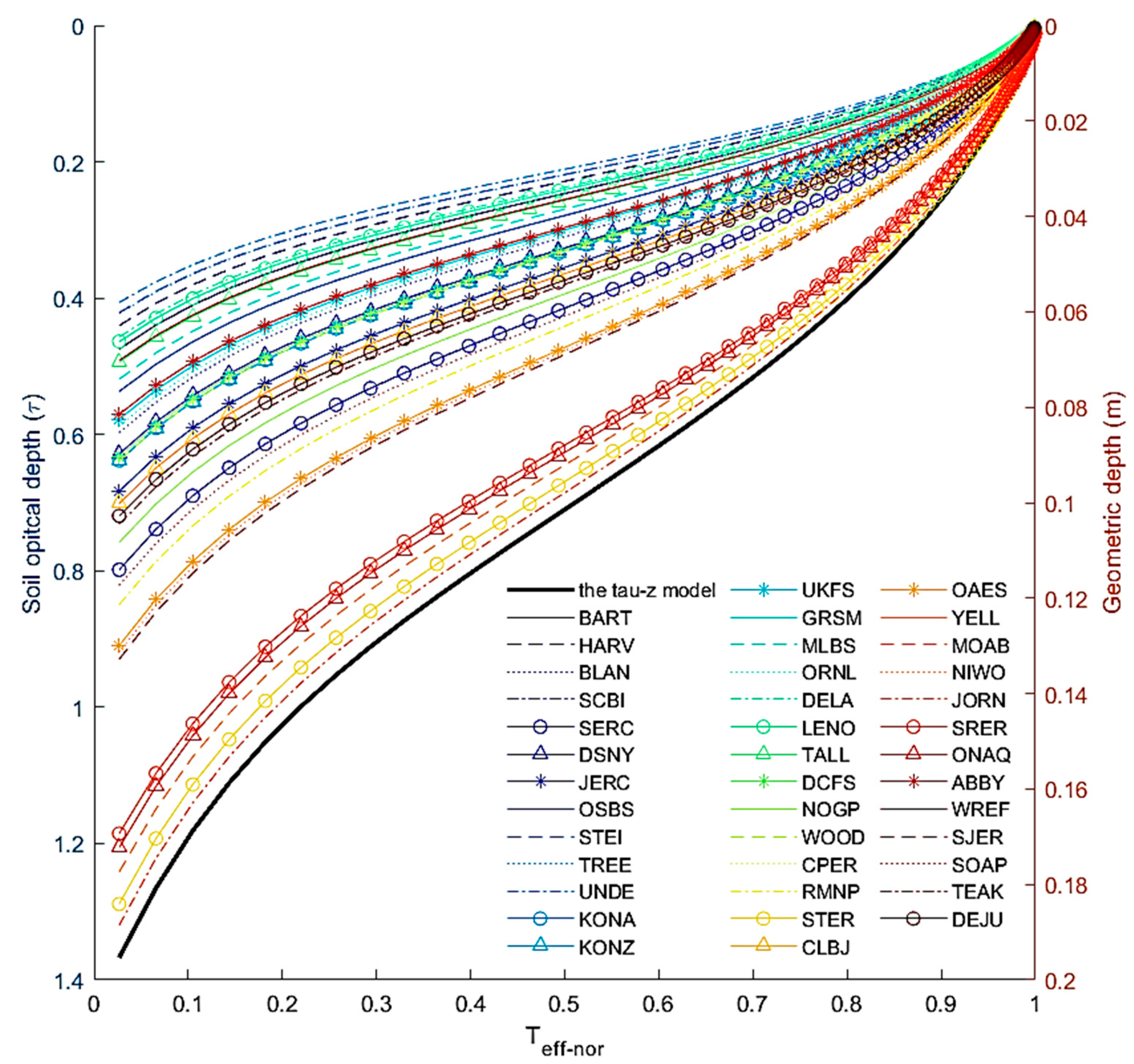
Figure 3 shows the τ-z model in the τ frame and its transformation to the z frame for each NEON site, along with their annual mean soil moisture from SMAP. zTeff ranges from 0 to 1.4 times the penetration depth (τ = 1) if the Teff_nor changes from 1 to 0. While the τ-z model shows a unique τ-Teff_nor relationship in τ, z depends on θ. With wet soil, zTeff would be shallower. For instance, when Teff_nor = 0.5, JORN (mean annual temperature (MAT): 15.7 °C, mean annual precipitation (MAP): 271 mm) would be zTeff = 0.1 m and zTeff = 0.025 m for UNDE (MAT: 4.3 °C, MAP: 802 mm). The zTeff shown in Figure 3 is based on an annual average θ from SMAP. Regarding a specified moment, zTeff should fit the average θ and may change according to the θ profile.
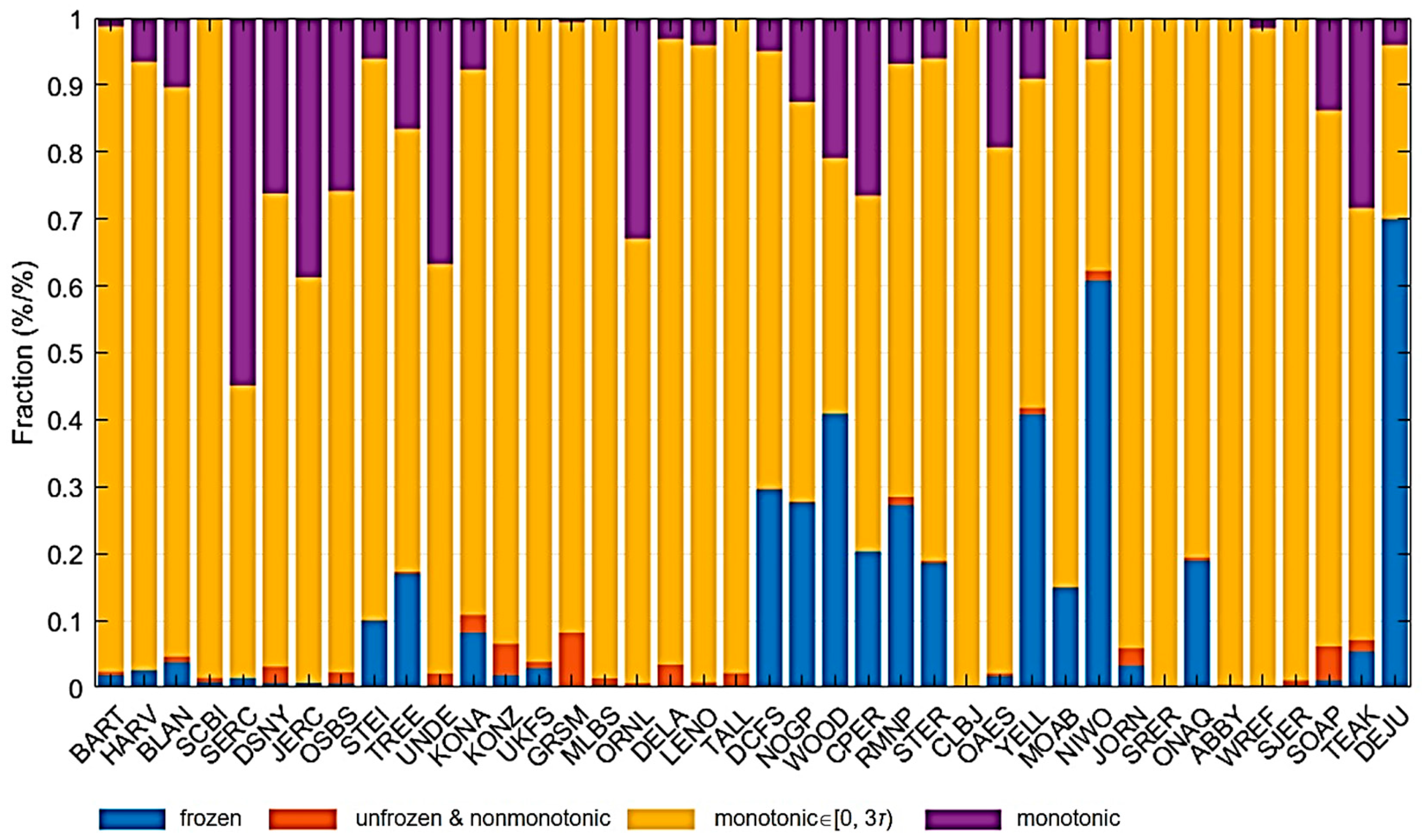
Figure 4 illustrates a quantitative analysis of categorical distributions across distinct climatic or experimental conditions, represented by four different color schemes. It should be noted that, on both short-term (diurnal) and long-term (seasonal) scales, soil temperature profiles generally exhibit distinct monotonic patterns under stable conditions: diurnally, surface temperatures fluctuate sharply due to solar radiation, while deeper layers (>10 cm) show smoother, near-monotonic decreases during the day and increases at night; seasonally, temperate regions typically display piecewise monotonicity, such as decreasing with depth in summer and increasing in winter.
However, these monotonic trends may break down in the presence of phase changes (e.g., freezing/thawing), abrupt moisture variations, or anthropogenic heat inputs, limiting the approach’s applicability under such conditions [30]. The blue hue signifies the ‘frozen’ state, which means the soil temperature profile contains at least one layer at ≤0 °C. The orange coloration represents the ‘unfrozen & nonmonotonic (i.e., the soil temperature profile is not monotonic in the vertical direction)’ category. The yellow tone indicates the ‘monotonic within three times the penetration depth (i.e., τ = 3 and e τ τ = 3 < 0.05, ‘monotonic ∈ [0, 3τ)’ in short heretheafter) category, where the orange satisfies the assumption roughly in τ. The profiles that strictly fit the assumption in the τ-z model are in purple, categorized as ‘monotonic’. The monotonic character is affected by soil thermal conductivity, moisture, type, color, structure, etc [31]. Generally, the τ-z model will work best for the monotonic category, followed sequentially by the orange, red, and blue categories. The bars, vertically aligned within their respective color zones, illustrate the proportional representation of each category within the corresponding condition. As expected, sites at higher latitudes and elevations tended to have more frozen conditions, and unfrozen and nonmonotonic conditions were rare at all sites.
Similarly, a more limited array of categories is represented in the ‘monotonic ∈ [0, 3τ)’ (orange) category, with notable variations in their proportional contributions. Lastly, the ‘monotonic’ (purple) category displays a narrower range of categories, each with a distinct proportionality, as indicated by the heights of their bars.

4.2. The Overall Performance

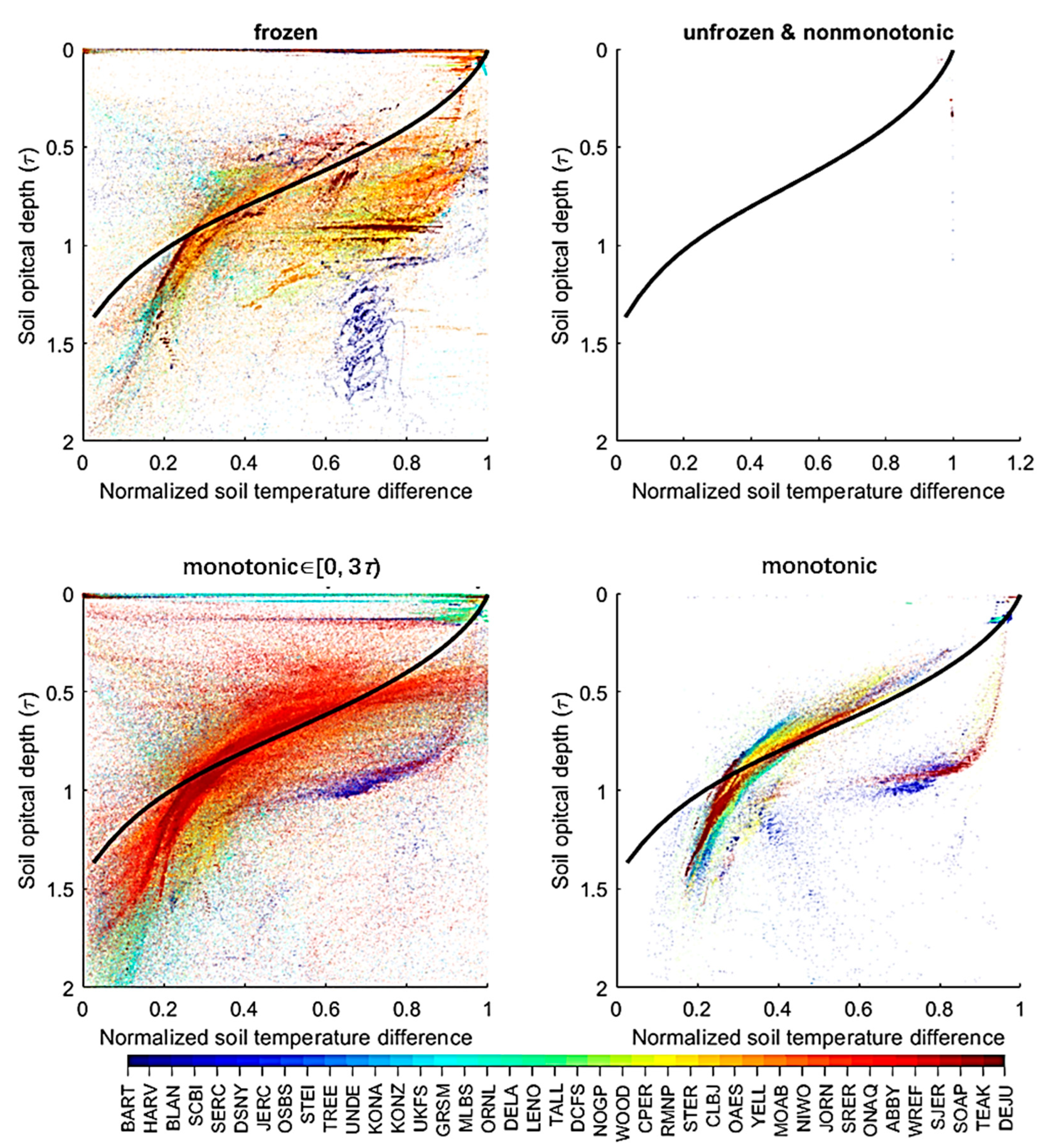
Upon categorizing the dataset into four distinct groups, as depicted in Figure 4, Figure 5 subsequently illustrates Teff_nor, alongside its intricate correlation with τ. The τ-z prediction model manifests as a standardized curve, invariant across all low-frequency microwave bands, encompassing various profile scenarios. Consequently, as a benchmark for subsequent evaluations, this τ-z curve remains constant across all subplots. We calculate τ based on the soil moisture and temperature profiles using Equations (3) and (4). Given that NEON sites encompass a maximum of nine layers for soil temperature and eight layers for soil moisture, we employ a rigorous linear interpolation methodology, incorporating exploration both towards the surface and to a depth of 2 m to derive a refined soil profile with enhanced precision. The real and imaginary parts of the dielectric constant can be acquired with various schemes, such as Mironov [32], which is a particular fit for the L-bands. While Mironov’s model (2009) offers superior accuracy for L-band frozen soils, Dobson’s model (1985) [33] was selected for its broader frequency applicability (0.3–3 GHz), inclusivity of soil textures, and computational efficiency, which are critical for large-scale validation across diverse ecosystems.
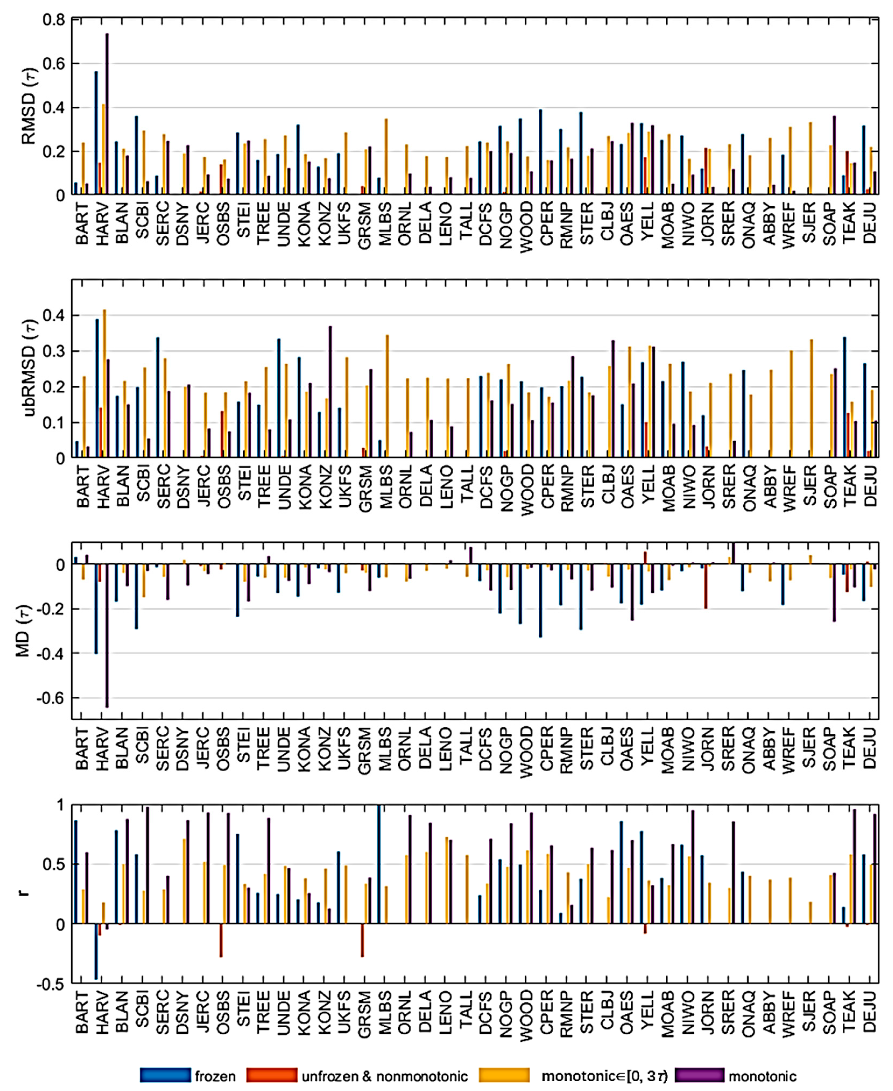
In the category of frozen soil, although the τ-z model is theoretically applicable to frozen conditions provided soil temperature exhibits monotonic behavior, accurately quantifying τ presents a formidable challenge due to the irregular scatter distribution. This issue is further exacerbated in the ‘unfrozen & nonmonotonic’ category, where the nonmonotonicity of the soil profile frequently results in Teff_nor falling outside the valid range [0, 1], rendering a significant portion of outlier points incompatible with the τ-z model. For the ‘monotonic ∈ [0, 3τ)’ category, the τ-z model exhibits good adherence with most scatter points, albeit with a notable presence of outliers. Although these outliers constitute a minor fraction, meticulous prefatory validation of the model’s applicability remains essential. The ‘monotonic’ category serves as a paradigm wherein soil profiles strictly adhere to the prerequisites of the τ-z model. An observation of this subset reveals that most points align closely with the τ-z curve within the range of [0.2, 0.8]. Notably, two exceptions arise: firstly, where the slope is steeper than the τ-z curve in the interval [0.2, 0.3], indicating a more rapid increase in τ than predicted; secondly, a distinct cluster of SOAP/CPER is marked in Italics because too few inputs are available. For the remaining 36 sites (Figure 5), the ‘monotonic’ case exhibits superior performance by markedly diminishing (RMSD) from 0.198/0.194 times τ to 0.110 (Table 1). Similarly, unRMSD is also reduced from 0.200/0.192 to 0.107.
Regarding Mean Difference (MD), the ‘frozen’ case demonstrates a bias of −0.132, whereas the other three cases present a comparable bias of approximately −0.04. Notably, r undergoes a substantial enhancement, escalating from approximately 0.496/0.444/0.454 for the remaining scenarios to 0.668 for the ‘monotonic’ case, indicating a stronger correlation between the observed and predicted values. Only OSBS and TEAK show negative r values, which is expected because the τ-z model does not fit the ‘unfrozen & nonmonotonic’.

4.3. The Performance at Individual Sites

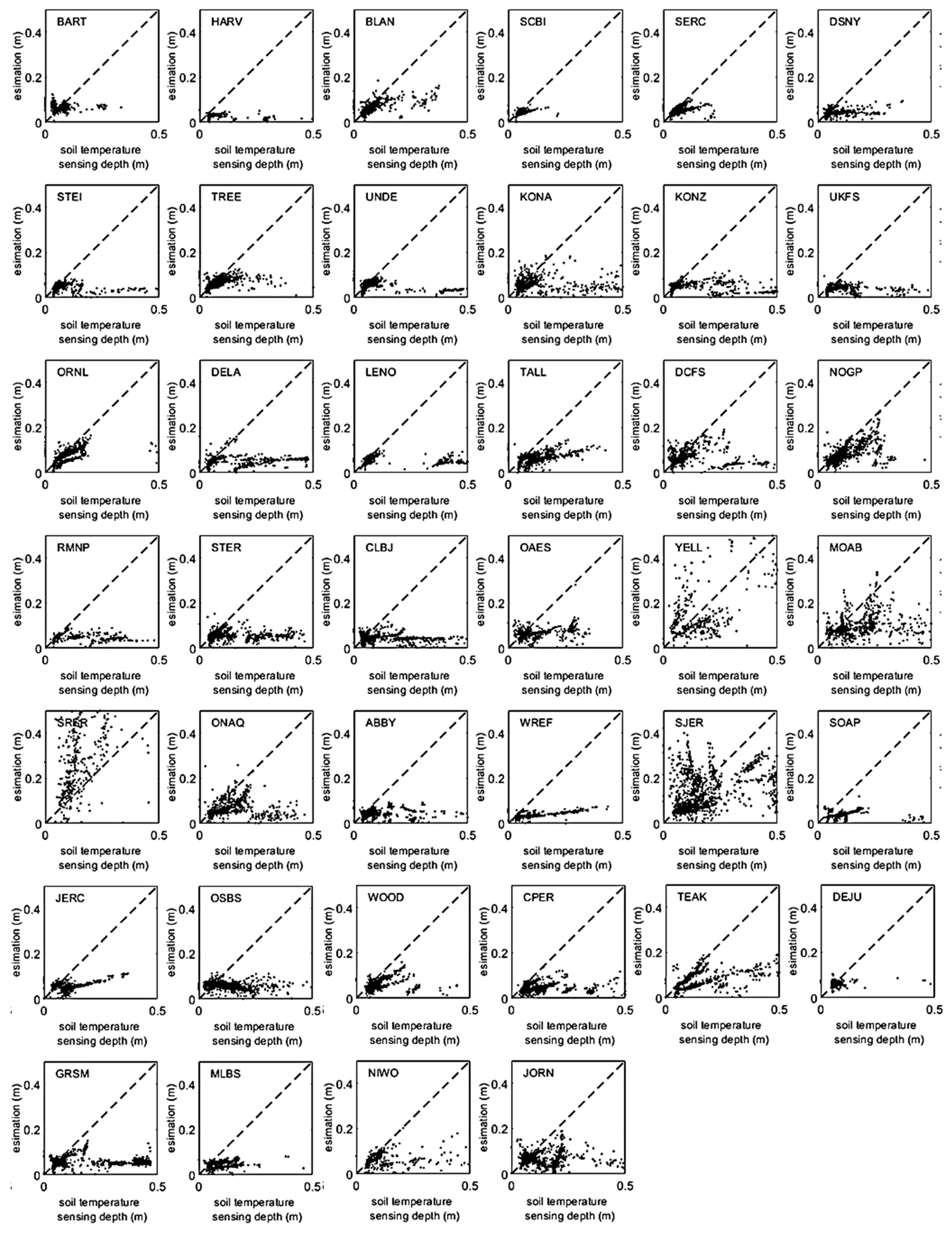
The NEON infrastructure encompasses a range of land surface types, including grasslands, forests, and shrublands/scrubs. Utilizing SMAP TB for these sites underscores its potential in retrieving θ. In this context, by substituting θ with SMAP-derived θ retrievals, we can derive zTeff estimates employing the τ-z model globally, and the estimation accuracy depends on the SMAP retrievals. In Figure 6, the zTeff/τTeff estimation is made directly through the τ-z model, and the validation depth is inferred from the soil profiles acquired by the NEON network. Based on the SMAP’s θ product, a comprehensive analysis of the scatter plot comparisons in Figure 7 reveals a diverse zTeff across multiple ecological sites.
Figure 6 presents multiple scatter plots, each uniquely representing a site (e.g., BLAN, JERC, STEI) and visually distinguished by τTeff in τ-z estimation. Each plot compares T against sensing depth inferred from the NEON profiles, elucidating the comparison between these variables. The densely distributed data points within each plot represent numerous measurements taken across various depths, illustrating a range of soil temperatures at different depths. Some sites exhibit tighter clusters of data points, reflecting a consistent relationship between soil temperature and depth (e.g., ORNL, TALL).
In contrast, others display more dispersed data points, indicating more significant variability in T profiles (e.g., YELL, MOAB). Across all sites, the zTeff varies significantly, with the lowest temperatures recorded at greater depths and the highest closer to the surface. θ derived from SMAP exhibits discrepancies with ground truth data for select sites, notably STEI, KONA, and NIWO, as evidenced in Figure 2 (bottom). For the remaining sites, the RMSD and unRMSD are observed to be less than 0.1 m, respectively, at locations such as JERC, TREE, MLBS, ORNL, WREF, and TEAK. The corresponding MD is also less than 0.05 m at most sites. Regarding r, over half of the sites exhibit negative values, indicating the need for meticulous scrutiny of the SMAP soil moisture estimates through rigorous validation procedures. This underscores the importance of cautiously applying SMAP soil moisture data in subsequent analyses.
Collectively, these scatter plots provide a comprehensive overview of zTeff variations with the estimation depth from SMAP, highlighting the complexity and uniqueness of T profiles in diverse environments. This information is vital for understanding the impact of T on ecological processes. It could inform the development of predictive models for T under varying climatic and environmental conditions. T has no significant contribution to the other layers in the emission [15]. The soil moisture or temperature at the penetration depth cannot represent the soil moisture or soil temperature used in Equation (9).
Furthermore, spatial and temporal variation complicates the TB signal at the L-band. θ varies spatially and temporally due to rainfall, evaporation, and vegetation cover. This heterogeneity poses challenges for satellite-based soil moisture retrieval algorithms, which often assume homogeneity over the spatial resolution of the sensor. Seen from the NEON network, each site consists of several sensors, and the data acquired from these sensors show different vertical structures. This increases the uncertainty in applying the τ-z model, although the accuracy of RMSD, unRMSD, and MD can reach 0.2 (τ) for most cases (Figure 5). In ‘monotonic’ conditions, the accuracy can even improve to 0.1 (τ). This means further analysis of zTeff or zθ is needed.
The third factor pertains to the contradiction between the geometric framework employed in the model-derived forward simulation for soil moisture retrieval and the τ framework. This discrepancy hinders a seamless transition from one framework to another, posing challenges in accurately describing and interpreting soil moisture retrieval processes. The soil moisture retrieval algorithms from satellite observations rely on various assumptions and models that may not fully capture the complexity of soil–microwave interactions. For example, the τ-z model, which explains the relationship between τ and Teff, does not accurately estimate the depths of soil moisture sensing. While the τ-z model can help investigate soil emission behavior in vertical structures, it does not always translate directly to precise soil moisture measurements.
In summary, the inconsistencies in θ estimates from satellite missions arise from several factors: uncertainties in microwave penetration depth, variations in space and time, algorithm limitations, instrumental constraints, and uncertainties in ground truth. Addressing these challenges requires a multidisciplinary approach that integrates advancements in sensor technology, algorithm development, and ground-based validation efforts.

5. Discussion

Although Figure 6 and Figure 7 show that the τ-z model exhibits robustness in the test data, several limitations constrain the model’s universal applicability.
First, its reliance on assumptions about monotonic temperature–depth relationships reduces accuracy in profiles with abrupt gradients, such as those influenced by rapid freezing/thawing cycles or layered soil textures. Second, spatial and temporal mismatches between coarse-resolution satellite data and point-scale ground observations introduce uncertainty, especially in heterogeneous landscapes where soil moisture dynamics vary sharply over short distances. Third, uncertainties in L-band passive microwave temperature sensing also arise from vegetation, surface roughness, snow cover, and limitations in depth validation. For instance, the vegetation canopy attenuates thermal emissions, with the L-band penetration depth decreasing by ~15% under dense forest cover, as demonstrated in boreal forest experiments [34]. Surface roughness induces emissivity variability, causing up to ±2 K errors in derived soil temperatures at 36 km resolution (compared to NEON’s 0.2 km2 sites), particularly in heterogeneous terrain [23]. Snow cover complicates thermal profiling by altering dielectric properties; in forested regions, snow–canopy interactions reduce temperature retrieval accuracy by ~22% [35]. These findings underscore the need for enhanced vegetation correction, refined roughness parameterization, and multi-scale validation to refine L-band temperature depth estimates.
A critical gap in L-band passive microwave remote sensing lies in the ambiguous conceptualization of sensing depth, which has inadvertently constrained the operational utility of SMAP and SMOS datasets. While prior studies frequently employ penetration depth metrics, these definitions remain inconsistent across the literature, ranging from electromagnetic attenuation coefficients to empirical thresholds, without empirical validation or standardized measurement protocols. This definitional ambiguity has led to a de facto neglect of the issue: no major satellite mission has publicly endorsed specific penetration depth formulations, and researchers often avoid explicit depth quantification in retrieval algorithms. In contrast, our work focuses exclusively on the physically grounded soil temperature effective sensing depth (zTeff), derived through harmonization of SMAP’s TB observations with NEON’s high-resolution (0–0.3 m) ground thermal profiles. By explicitly accounting for soil state transitions (e.g., thawing fronts)—which previous studies either oversimplified or treated as edge cases—we achieve an RMSD of 0.05 m (unRMSD 0.1 m) in zTeff estimation across diverse ecosystems. This represents a marked improvement over models relying on vague penetration depth concepts, which typically exhibit errors greater than 0.3 m in heterogeneous landscapes.

6. Conclusions

The τ-z model provides a rigorous mathematical framework for estimating zTeff, where observed soil temperature (T) aligns with its effective counterpart (Teff). This study advances prior validations—such as those by [15,21]—by demonstrating the model’s robustness across a broader spectrum of soil conditions (e.g., monotonic, frozen, and nonmonotonic profiles) and spatial scales, leveraging high-temporal-resolution data from NEON and SMAP. These results highlight the model’s operational potential for global soil moisture validation, particularly in regions with limited in situ measurements—a critical advancement for enhancing the reliability of L-band remote sensing missions.
Our multi-scale validation approach yields three interconnected insights into the τ-z model’s performance. First, the model demonstrates exceptional accuracy under monotonic soil conditions, where temperature gradients align predictably with depth. In homogeneous soil profiles, the model demonstrates robust performance, with both RMSD and unRMSD stabilizing at 0.11 τ. Concurrently, the correlation coefficient (r) improves from 0.4 to 0.69, indicating stronger agreement between modeled and observed data. Notably, the model’s adaptability is most evident in heterogeneous conditions, such as frozen soils or transiently thawed layers. Even under these complex scenarios, accuracy remains acceptable, with RMSD values approximately 0.2 τ. This suggests the τ-z framework effectively captures complex soil moisture dynamics, even when temperature–depth relationships deviate from idealized assumptions.
By addressing limitations of prior works through multi-scale, categorical validation, this study sets a new benchmark for evaluating soil moisture retrieval models. The findings enhance confidence in the τ-z model’s applicability across agriculture, hydrology, and climate science, offering a pathway toward more accurate Earth system monitoring using multi-source remote sensing data. For instance, it shows that a TB trend in the Antarctic continent observed by SMAP may not be due to a temperature increase in the ice sheet, but rather to various zTeff values [36].

Author Contributions

Conceptualization, S.L.; methodology, S.L.; software, S.L.; validation, S.L., E.A. and Y.H.; formal analysis, S.L.; investigation, S.L.; resources, S.L.; data curation, S.L., E.A. and Y.H.; writing—original draft preparation, S.L.; writing—review and editing, S.L. and Y.H.; visualization, S.L.; supervision, E.A.; project administration, S.L.; funding acquisition, S.L. All authors have read and agreed to the published version of the manuscript.

Funding

This research was funded by the Key Research and Development and Achievement Transformation Program of Inner Mongolia Autonomous Region, China (Grant No. 2025YFDZ0007), the Yan Liyuan–ENSKY Foundation Project of Zhuhai Fudan Innovation Research Institute (Grant No. JX240002), the National Key R&D Program of China (Grant No. 2022YFF0801404), and the National Natural Science Foundation of China (Grant No. 42075150). The National Ecological Observatory Network is a program sponsored by the US National Science Foundation and operated under a cooperative agreement by Battelle. This material is partly based on work supported by the US National Science Foundation through the NEON Program.

Data Availability Statement

NEON’s soil temperature and moisture datasets can be accessed through NEON’s online portal (https://www.neonscience.org/data-collection/soils, provided by Edward Ayres via email on 1 October 2024). SMAP soil moisture data can be accessed at https://nsidc.org/data/spl3smp/versions/8, spanning from July 2019 to June 2022 (accessed on 1 October 2024).

Acknowledgments

We sincerely appreciate all the contributors to the dataset used in this study.

Conflicts of Interest

The authors declare no conflicts of interest.

References

  1. Wigneron, J.P.; Jackson, T.J.; O’Neill, P.; De Lannoy, G.; de Rosnay, P.; Walker, J.P.; Ferrazzoli, P.; Mironov, V.; Bircher, S.; Grant, J.P.; et al. Modelling the passive microwave signature from land surfaces: A review of recent results and application to the L-band SMOS & SMAP soil moisture retrieval algorithms. Remote Sens. Environ. 2017, 192, 238–262. [Google Scholar] [CrossRef]
  2. Cho, E.; Jacobs, J.M.; Schroeder, R.; Tuttle, S.E.; Olheiser, C. Improvement of operational airborne gamma radiation snow water equivalent estimates using SMAP soil moisture. Remote Sens. Environ. 2020, 240, 111668. [Google Scholar] [CrossRef]
  3. Li, X.; Wigneron, J.-P.; Fan, L.; Frappart, F.; Yueh, S.H.; Colliander, A.; Ebtehaj, A.; Gao, L.; Fernandez-Moran, R.; Liu, X.; et al. A new SMAP soil moisture and vegetation optical depth product (SMAP-IB): Algorithm, assessment and inter-comparison. Remote Sens. Environ. 2022, 271, 112921. [Google Scholar] [CrossRef]
  4. Zhao, H.; Montzka, C.; Baatz, R.; Vereecken, H.; Franssen, H.-J.H. The Importance of Subsurface Processes in Land Surface Modeling over a Temperate Region: An Analysis with SMAP, Cosmic Ray Neutron Sensing and Triple Collocation Analysis. Remote Sens. 2021, 13, 3068. [Google Scholar] [CrossRef]
  5. Dirmeyer, P.A.; Norton, H.E. Indications of Surface and Sub-Surface Hydrologic Properties from SMAP Soil Moisture Retrievals. Hydrology 2018, 5, 36. [Google Scholar] [CrossRef]
  6. Kerr, Y.H.; Waldteufel, P.; Wigneron, J.P.; Delwart, S.; Cabot, F.; Boutin, J.; Escorihuela, M.J.; Font, J.; Reul, N.; Gruhier, C.; et al. The SMOS Mission: New Tool for Monitoring Key Elements of the Global Water Cycle. Proc. IEEE 2010, 98, 666–687. [Google Scholar] [CrossRef]
  7. Entekhabi, D.; Njoku, E.G.; Neill, P.E.O.; Kellogg, K.H.; Crow, W.T.; Edelstein, W.N.; Entin, J.K.; Goodman, S.D.; Jackson, T.J.; Johnson, J.; et al. The Soil Moisture Active Passive (SMAP) Mission. Proc. IEEE 2010, 98, 704–716. [Google Scholar] [CrossRef]
  8. Cui, K.; Xing, M.; Shang, J.; Zhou, X.; Wang, J. Enhanced L-MEB Model for Soil Moisture Retrieval Over Soybean Fields During the Growing Season. IEEE Trans. Geosci. Remote Sens. 2025, 63, 1–16. [Google Scholar] [CrossRef]
  9. Xing, M.; Cui, K.; Dong, T.; Ma, M.; Zhou, X.; Zhang, Y. Improved soil moisture retrieval during crop growing season using passive microwave data at L-band. Int. J. Appl. Earth Obs. Geoinf. 2025, 143, 104788. [Google Scholar] [CrossRef]
  10. Bhogapurapu, N.; Dey, S.; Mandal, D.; Bhattacharya, A.; Karthikeyan, L.; McNairn, H.; Rao, Y.S. Soil moisture retrieval over croplands using dual-pol L-band GRD SAR data. Remote Sens. Environ. 2022, 271, 112900. [Google Scholar] [CrossRef]
  11. Ma, H.; Zeng, J.; Zhang, X.; Peng, J.; Li, X.; Fu, P.; Cosh, M.H.; Letu, H.; Wang, S.; Chen, N.; et al. Surface soil moisture from combined active and passive microwave observations: Integrating ASCAT and SMAP observations based on machine learning approaches. Remote Sens. Environ. 2024, 308, 114197. [Google Scholar] [CrossRef]
  12. Li, Z.; Yang, Q.; Li, J.; Jin, T.; Yuan, Q.; Shen, H.; Zhang, L. Global multi-scale surface soil moisture retrieval coupling physical mechanisms and machine learning in the cloud environment. Remote Sens. Environ. 2025, 329, 114928. [Google Scholar] [CrossRef]
  13. Colliander, A.; Jackson, T.J.; Chan, S.K.; O’Neill, P.; Bindlish, R.; Cosh, M.H.; Caldwell, T.; Walker, J.P.; Berg, A.; McNairn, H.; et al. An assessment of the differences between spatial resolution and grid size for the SMAP enhanced soil moisture product over homogeneous sites. Remote Sens. Environ. 2018, 207, 65–70. [Google Scholar] [CrossRef]
  14. Chan, S.K.; Bindlish, R.; O’Neill, P.E.; Njoku, E.; Jackson, T.; Colliander, A.; Chen, F.; Burgin, M.; Dunbar, S.; Piepmeier, J.; et al. Assessment of the SMAP Passive Soil Moisture Product. IEEE Trans. Geosci. Remote Sens. 2016, 54, 4994–5007. [Google Scholar] [CrossRef]
  15. Lv, S.; Zhao, T.; Hu, Y.; Wen, J. Empirical Validation of Soil Temperature Sensing Depth Derived from the Tau-z Model Utilizing Data from the Soil Moisture Experiment in the Luan River (SMELR). IEEE J. Sel. Top. Appl. Earth Obs. Remote Sens. 2024, 17, 14742–14751. [Google Scholar] [CrossRef]
  16. Macelloni, G.; Leduc-Leballeur, M.; Montomoli, F.; Brogioni, M.; Ritz, C.; Picard, G. On the retrieval of internal temperature of Antarctica Ice Sheet by using SMOS observations. Remote Sens. Environ. 2019, 233, 111405. [Google Scholar] [CrossRef]
  17. Brakhasi, F.; Walker, J.P.; Ye, N.; Wu, X.; Shen, X.; Yeo, I.-Y.; Boopathi, N.; Kim, E.; Kerr, Y.; Jackson, T. Towards soil moisture profile estimation in the root zone using L- and P-band radiometer observations: A coherent modelling approach. Sci. Remote Sens. 2023, 7, 100079. [Google Scholar] [CrossRef]
  18. Ulaby, F.T.; Moore, R.K.; Fung, A.K. Microwave Remote Sensing Active and Passive-Volume II: Radar Remote Sensing and Surface Scattering and Emission Theory; Addison-Wesley Publishing Company Advanced Book Program/World Science Division: Reading, MA, USA; Norwood, MA, USA, 1982. [Google Scholar]
  19. Bindlish, R. Active and Passive Microwave Remote Sensing of Soil Moisture; The Pennsylvania State University: University Park, PA, USA, 2000. [Google Scholar]
  20. Taheri, M.; Schreiner, H.K.; Mohammadian, A.; Shirkhani, H.; Payeur, P.; Imanian, H.; Cobo, J.H. A Review of Machine Learning Approaches to Soil Temperature Estimation. Sustainability 2023, 15, 7677. [Google Scholar] [CrossRef]
  21. Lv, S.; Zeng, Y.; Su, Z.; Wen, J. A Closed-Form Expression of Soil Temperature Sensing Depth at L-Band. IEEE Trans. Geosci. Remote Sens. 2019, 57, 4889–4897. [Google Scholar] [CrossRef]
  22. Goodman, K.J.; Parker, S.M.; Edmonds, J.W.; Zeglin, L.H. Expanding the scale of aquatic sciences: The role of the National Ecological Observatory Network (NEON). Freshw. Sci. 2015, 34, 377–385. [Google Scholar] [CrossRef]
  23. Ayres, E.; Reichle, R.H.; Colliander, A.; Cosh, M.H.; Smith, L. Validation of Remotely Sensed and Modeled Soil Moisture at Forested and Unforested NEON Sites. IEEE J. Sel. Top. Appl. Earth Obs. Remote Sens. 2024, 17, 14248–14264. [Google Scholar] [CrossRef]
  24. Brakhasi, F.; Walker, J.P.; Judge, J.; Liu, P.-W.; Shen, X.; Ye, N.; Wu, X.; Yeo, I.-Y.; Kim, E.; Kerr, Y.; et al. Soil moisture profile estimation under bare and vegetated soils using combined L-band and P-band radiometer observations: An incoherent modeling approach. Remote Sens. Environ. 2024, 307, 114148. [Google Scholar] [CrossRef]
  25. Ayres, E.; Colliander, A.; Cosh, M.H.; Roberti, J.A.; Simkin, S.; Genazzio, M.A. Validation of SMAP Soil Moisture at Terrestrial National Ecological Observatory Network (NEON) Sites Show Potential for Soil Moisture Retrieval in Forested Areas. IEEE J. Sel. Top. Appl. Earth Obs. Remote Sens. 2021, 14, 10903–10918. [Google Scholar] [CrossRef]
  26. Wilheit, T.T. Radiative transfer in a plane stratified dielectric. IEEE Trans. Geosci. Remote Sens. 1978, 16, 138–143. [Google Scholar] [CrossRef]
  27. Lv, S.; Wen, J.; Zeng, Y.; Tian, H.; Su, Z. An improved two-layer algorithm for estimating effective soil temperature in microwave radiometry using in situ temperature and soil moisture measurements. Remote Sens. Environ. 2014, 152, 356–363. [Google Scholar] [CrossRef]
  28. Moriasi, D.N.; Arnold, J.G.; Liew, M.W.V.; Bingner, R.L.; Harmel, R.D.; Veith, T.L. Model Evaluation Guidelines for Systematic Quantification of Accuracy in Watershed Simulations. Trans. ASABE 2007, 50, 885–900. [Google Scholar] [CrossRef]
  29. Pearson, K., VII. Note on regression and inheritance in the case of two parents. Proc. R. Soc. Lond. 1997, 58, 240–242. [Google Scholar] [CrossRef]
  30. Holmes, T.R.H.; Owe, M.; De Jeu, R.A.M.; Kooi, H. Estimating the soil temperature profile from a single depth observation: A simple empirical heatflow solution. Water Resour. Res. 2008, 44, W02412. [Google Scholar] [CrossRef]
  31. Hinzman, L.D.; Goering, D.J.; Kane, D.L. A distributed thermal model for calculating soil temperature profiles and depth of thaw in permafrost regions. J. Geophys. Res. Atmos. 1998, 103, 28975–28991. [Google Scholar] [CrossRef]
  32. Mironov, V.L.; Kosolapova, L.G.; Fomin, S.V. Physically and Mineralogically Based Spectroscopic Dielectric Model for Moist Soils. IEEE Trans. Geosci. Remote Sens. 2009, 47, 2059–2070. [Google Scholar] [CrossRef]
  33. Dobson, M.C.; Ulaby, F.T.; Hallikainen, M.T.; El-rayes, M.A. Microwave Dielectric Behavior of Wet Soil-Part II: Dielectric Mixing Models. IEEE Trans. Geosci. Remote Sens. 1985, GE-23, 35–46. [Google Scholar] [CrossRef]
  34. Li, M.; Lang, R.; Cosh, M. P-Band and L-Band Radiometry Retrieval of Soil Moisture and Temperature Profiles. IEEE Trans. Geosci. Remote Sens. 2024, 62, 1–15. [Google Scholar] [CrossRef]
  35. Schwank, M.; Rautiainen, K.; Mätzler, C.; Stähli, M.; Lemmetyinen, J.; Pulliainen, J.; Vehviläinen, J.; Kontu, A.; Ikonen, J.; Ménard, C.B. Model for microwave emission of a snow-covered ground with focus on L band. Remote Sens. Environ. 2014, 154, 180–191. [Google Scholar] [CrossRef]
  36. Lv, S.; Hu, Y.; Wen, J. Decadal-Scale Warming Signals in Antarctic Ice Sheet Interior Revealed by L-Band Passive Microwave Observations. Remote Sens. 2025, 17, 3757. [Google Scholar] [CrossRef]
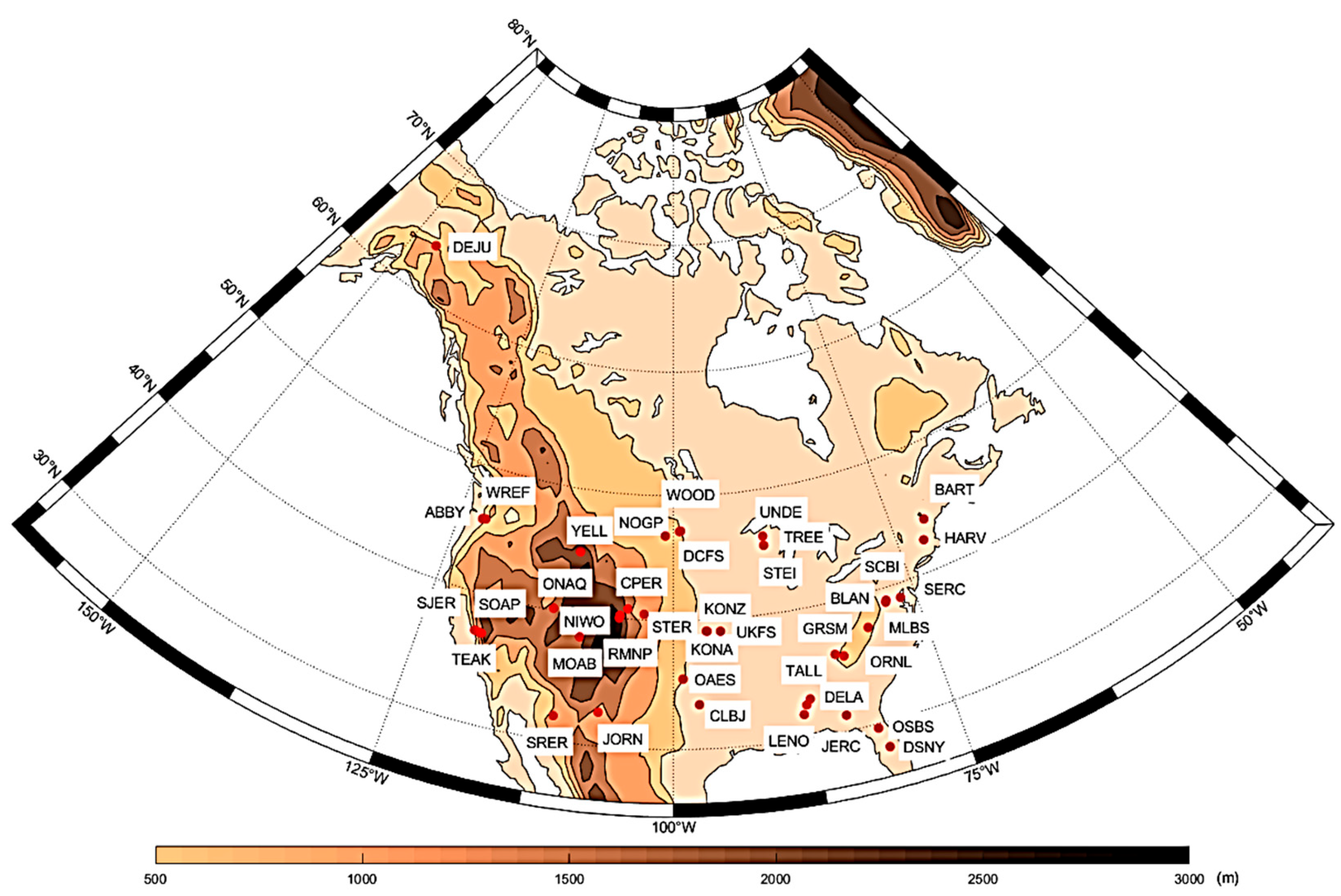
Figure 1. The locations and elevation of the 40 sites collected by NEON in this study. The color bar shows the elevation map.
Remotesensing 17 03845 g001
Figure 2. Violin plots comparing soil temperature and moisture distributions from NEON ground-based profiles (green and red) and SMAP satellite observations (blue). Each plot displays the kernel density-smoothed distribution (represented by the violin shape) for both datasets.
Remotesensing 17 03845 g002
Figure 3. The τ-z model and the soil temperature sensing depth (zTeff) inferred from SMAP soil moisture data and soil texture data from each NEON site.
Remotesensing 17 03845 g003
Figure 4. The categories analyzed include the fraction of frozen soil, unfrozen and nonmonotonic soil profiles, monotonic ∈ [0, 3τ), and monotonic soil behavior.
Remotesensing 17 03845 g004
Figure 5. The relationship between the Teff_nor and τ was evaluated against the τ-z model across 40 sites within the National Ecological Observatory Network (NEON). The black line represents the τ-z model predictions, while the individual data points, colored to differentiate between various sites, serve to illustrate the model’s performance against the empirical data.
Remotesensing 17 03845 g005
Figure 6. The soil temperature sensing depth comparison inferred from Equation (9) using SMAP data, compared to the one from the NEON profile. The dotted line is a 1:1 ratio reference.
Remotesensing 17 03845 g006
Figure 7. The compilation of the Teff_nor and τ relation test against the τ-z model at 40 sites under four soil conditions.
Remotesensing 17 03845 g007
Table 1. The statistics for Figure 5. The ‘unfrozen & nonmonotonic’ is marked in Italics because too few inputs are available.
FrozenUnfrozen & NonmonotonicMonotonic ∈ [0, 3τ)Monotonic
RMSD (τ)0.2940.0270.2150.149
unRMSD (τ)0.0950.0180.2180.168
MD (τ) Dobson−0.094−0.012−0.040−0.064
PearsonCC0.205−0.0220.4870.695
Disclaimer/Publisher’s Note: The statements, opinions and data contained in all publications are solely those of the individual author(s) and contributor(s) and not of MDPI and/or the editor(s). MDPI and/or the editor(s) disclaim responsibility for any injury to people or property resulting from any ideas, methods, instructions or products referred to in the content.