Highlights
What are the main findings?
- NPPCast outperforms UNet-family models and CESM2 hindcasts across most leads and regions.
- NPPCast maintains robust skill across different pretraining datasets.
What is the implication of the main finding?
- NPPCast offers a reliable framework for seasonal-to-multiyear ocean net primary production forecasting.
- The results support advances in climate prediction and ecosystem management.
Abstract
Skillful prediction of marine net primary production (NPP) on seasonal to multi-year timescales is essential for assessing the ocean’s role in the global carbon cycle and managing marine resources. We introduce NPPCast, a compact convolutional neural network using causal dilated convolutions, and compare its performance with four representative UNet-family models (UNet, VNet, AttUNet, R2UNet). Each model is pre-trained on 36-month output from either Community Earth System Model version 2 forced-ocean–sea-ice (CESM2-FOSI) or interannual varying forcing (CESM2-GIAF) and fine-tuned using three satellite-derived NPP products (the Standard Vertically Generalized Production Model (SVGPM), the Eppley Vertically Generalized Production Model (EVGPM), and the Carbon-based Productivity Model (CbPM)) as well as their multi-product mean (MEAN). Across most tests, NPPCast outperforms the baselines, reducing global root mean square error (RMSE) by 30–56% on MEAN/EVGPM/SVGPM and improving the anomaly correlation coefficient (ACC) by 0.32–0.49 over the best UNet-based alternative. NPPCast also achieves the highest structural similarity to observations and low bias, as seen in scatter and spatial analyses, and attains the highest or tied-highest Nash–Sutcliffe efficiency (NSE) in three of four products. Crucially, NPPCast’s performance remains stable when switching between FOSI and GIAF pre-training datasets, with RMSE changing by at most 2.17%, whereas UNet-family models vary from −41.6% to +42.5%. We show that NPPCast consistently outperforms the Earth system model, sustaining significant predictive skill in contrast to the rapid decline observed in the latter. These results demonstrate that an architecture that maintains performance across different pre-training datasets (CESM2–FOSI and CESM2–GIAF) can yield more accurate and reliable long-range global NPP forecasts than UNet-family models.
1. Introduction
Net primary production (NPP) in the ocean, the net amount of organic carbon produced by phytoplankton through photosynthesis after subtracting respiration, accounts for approximately half of the global NPP []. As a critical component of the global carbon cycle, NPP drives the biological carbon pump, which transfers carbon to the deep ocean where it can be sequestered in sediments, thereby helping to regulate atmospheric carbon dioxide levels and mitigate climate change []. Moreover, NPP is the foundation of the marine food web and has a profound influence on the sustainability of fishery resources and the conservation of biodiversity [].
With the advancement of satellite ocean-color remote sensing, various algorithmic models have been developed to estimate NPP. Among them, the Vertical Generalized Production Model (VGPM) is one of the most widely applied, estimating depth-integrated NPP from surface chlorophyll, sea surface temperature, photosynthetically available radiation (PAR), and the euphotic depth []. Given uncertainties associated with satellite-derived chlorophyll concentrations, Behrenfeld et al. [] introduced the Carbon-based Productivity Model (CbPM), which replaces chlorophyll with phytoplankton carbon—derived from the particle backscattering coefficient to estimate NPP. This approach was later refined by Westberry et al. [], who introduced a spectrally resolved light attenuation scheme, to better represent the underwater light field. Additionally, Lee et al. [] developed the Absorption-based Productivity Model (AbPM), which estimates NPP from the absorption of solar radiation by phytoplankton, using satellite-derived absorption coefficients and PAR. Despite these advances, such models remain limited by their reliance on satellite observations, highlighting the need for predictive approaches capable of forecasting NPP under varying environmental and climate conditions.
Previously, NPP was commonly predicted using numerical modeling approaches that incorporated key controlling factors in the ocean, such as temperature, light availability, nutrient concentrations, and mixed layer depth [,,]. Many studies have evaluated the potential predictability of NPP, that is, the theoretical upper limit of forecast model performance under idealized conditions. Séférian et al. [] demonstrated that forecast models can predict NPP variability in the tropical Pacific Ocean up to three years in advance, highlighting the key role of nutrient advection processes. Krumhardt et al. [] showed that NPP is predictable up to 1 to 3 years ahead in many ocean regions, with nutrient-driven areas exhibiting higher predictability than those primarily influenced by light or temperature. Furthermore, Frölicher et al. [] found that the potential predictability of NPP is approximately three years, and indicated that predictability in mid-latitude regions is mainly governed by nutrient limitations, while high-latitude regions are predominantly influenced by temperature and light limitations. These studies reveal that NPP has certain potential predictability within 3 years and highlight the dominant role of key environmental factors in regional predictability.
However, systematic evaluations on actual prediction skill of NPP remain limited. Prediction skill refers to the model’s ability to accurately reproduce observed results under real-world conditions, typically quantified by comparing model outputs with observational data []. Several key factors constrain progress in this area, such as limited biogeochemical observation coverage [], process and parameter uncertainties in models [,,], data assimilation challenges due to the timeliness, sparsity, and diversity of observation data [], and the high computational cost of retrospective forecasts []. These factors significantly hinder the advancement of actual prediction skill assessments for NPP, and pose a huge challenge on global ocean NPP forecasting. Another challenge is the Spring Predictability Barrier (SPB) [], where the prediction skill for El Niño–Southern Oscillation (ENSO), and thus, for key environmental drivers such as light availability and nutrient supply, drops significantly during the boreal spring primarily due to the seasonal weakening of ENSO signals and rapid amplification of initial condition errors [,,]. This could further degrade NPP forecasts with traditional Earth system models.
With the rapid development of Artificial Intelligence (AI), especially the widespread application of deep learning, significant potential has emerged for its use in marine sciences and NPP prediction [,,]. Deep learning offers a promising alternative, with the ability to model complex nonlinear relationships and handle large, nonlinear, and spatiotemporally dependent datasets. Moreover, compared to traditional numerical models, deep learning has significant advantages in computational efficiency.
Recent years, UNet-based architectures—UNet, V-Net, Attention-UNet, and R2-UNet—have been widely applied to oceanic prediction tasks. A sea-surface-temperature UNet described by Ren et al. [], for example, employs skip connections to aggregate multi-scale context and attains notable skill, yet its encoder–decoder structure often blurs sharp coastal gradients and entails a large GPU footprint. Attention gates and residual blocks partially alleviate these issues: the RA-UNet sharpened ocean-precipitation nowcasts and marine-debris masks [,], but residual artifacts persist in high-gradient regions. Likewise, R2-UNet’s residual-recurrent scheme deepens the receptive field and mitigates vanishing gradients, boosting flood and sea-ice mapping accuracy [], yet it still yields overly smooth predictions in homogeneous water masses.
Despite their multi-scale context aggregation, three methodological issues restrict UNet-based models’ suitability for global NPP forecasting. First, large receptive fields tend to smooth productive hotspots in upwelling zones and marginal seas, even when physics-informed losses are imposed. Second, the pointwise attribution is opaque: a grid-cell prediction inherits information from an implicit data-driven neighbourhood, hampering mechanistic interpretation of NPP forecasting. Third, and most critically for operational transfer, the networks’ skill hinges on the provenance of their pre-training data—the same architecture fine-tuned on a mismatched source often degrades markedly, whereas careful source–target pairing can recover 1–5% RMSE or MAE [,]. Such sensitivity complicates large-scale roll-outs, where historical simulations and observations differ across basins. However, systematic evaluation of the actual prediction skill of marine NPP using deep learning approaches remains at an early stage.
Therefore, a globally transferable model that retains high spatial fidelity, interpretability, and stable skill across diverse pre-training scenes is still lacking. Here, we introduce NPPCast, an architecture that recasts large-scale spatio-temporal prediction as a family of grouped multivariate time-series problems. We evaluate the predictability of NPPCast contained in the NPP field itself at 12–36-month leads. This target-only design gives a transparent baseline and uniform global coverage.
The model (i) employs causal dilated convolutions and highway connections instead of an encoder–decoder upsampling pathway, thereby preserving fine-scale gradients without over-smoothing; (ii) expresses each grid-cell forecast as an explicit depth-wise-separable convolution over the previous 36 months; and (iii) is deliberately designed to maintain accuracy across various pre-training and fine-tuning datasets. A rigorous evaluation over 36 forecast leads, incorporating anomaly correlation coefficient (ACC), root mean square error (RMSE), mean absolute error (MAE), Nash–Sutcliffe efficiency (NSE), structural similarity index (SSIM), annual-mean bias, and spatial Hovmöller diagnostics, demonstrates that NPPCast consistently outperforms UNet, V-Net, Attention-UNet, and R2-UNet across all metrics and retains its advantage regardless of pre-training scenes. In addition, NPPCast is evaluated across multiple satellite-derived NPP product families, including the chlorophyll-based VGPM and the carbon-based CbPM to assess its robustness to mechanistically distinct targets. These results provide the first systematic benchmark of deep networks for global marine NPP prediction and show that a compact, interpretable architecture can surpass much deeper encoder–decoder CNNs in both accuracy and efficiency.
2. Materials and Methods
2.1. Data Information
2.1.1. Model Data
CESM2-FOSI and CESM2-GIAF are outputs of two simulations based on the “ocean and sea ice” coupled configuration within the CESM2 framework, covering the period of 1958–2020 and 1958–2018, respectively. Both experiments use atmospheric fields from the Japanese 55-year atmospheric reanalysis dataset (JRA55-do) as surface boundary conditions to drive the evolution of ocean and sea ice components []. While CESM2-FOSI and CESM2-GIAF are largely consistent in model resolution, component configuration, and forcing data sources, they exhibit notable differences in the specification of certain key physical parameters, including sea ice albedo, sea surface temperature (SST) restoring, and deep-ocean diffusion []. In this study, we extracted NPP from two datasets to pre-train the model. The CESM2-SMYLE (Seasonal-to-Multiyear Large Ensemble) is a set of initialized climate predictions based on CESM2, designed to investigate Earth system predictability on timescales ranging from one month to two years. Covering the period from 1970 to 2019, the system performs four initializations per year, each with 20 ensemble members, generating two-year-long hindcasts. CESM2-SMYLE provides comprehensive output across all major Earth system components for studying near-term climate variability and its impacts. More information can be found in []. CESM2-SMYLE is used as a reference to provide context for evaluating the performance of NPPCast. The CESM2 dataset used in this study features a horizontal spatial resolution of approximately , which corresponds to a grid spacing of about 110 km × 110 km in equatorial regions.
2.1.2. Satellite Observation Data
SVGPM, EVGPM, and CbPM are three widely used satellite-based algorithms for ocean NPP. VGPM is a chlorophyll-based model that estimates NPP using a temperature-dependent description of chlorophyll-specific photosynthetic efficiency. Its key input variables include chlorophyll concentration, light availability, and photosynthetic efficiency []. Building on this, Eppley-VGPM incorporates the Eppley temperature function, which allows for a more continuous and physiologically realistic temperature-efficiency relationship across different thermal regimes [,,]. In contrast, the CbPM model estimates NPP directly from phytoplankton carbon biomass and growth rate, while also accounting for light availability and photoacclimation processes. This approach makes it more consistent with the physiological processes of phytoplankton [,]. These three models differ in algorithmic structure, input variables, and applicable conditions, and are often used for comparative studies of marine NPP. The spatial resolution of the satellite observation data used in this study is approximately 9 km. To ensure consistency and comparability, the satellite data were interpolated to the spatial grid of the CESM2 model for subsequent analyses. All satellite data can be downloaded at https://earth.gsfc.nasa.gov/ocean/data/ocean-productivity-data-server (accessed on 1 November 2025).
2.2. NPPCast Framework
In this work, we propose NPPCast, a novel framework that reformulates large-scale spatiotemporal forecasting as a set of grouped multivariate time series forecasting problems (Figure 1). Instead of applying a single monolithic model over an entire spatial field, NPPCast first leverages an ocean–land mask to reconstruct the input into a sparse representation, then partitions the domain into multiple regional groups, and finally deploys dedicated time-series models for each region. This design ensures that each model focuses on the local dynamics of its region while ignoring irrelevant areas, thereby improving both efficiency and predictive fidelity. In summary, NPPCast’s workflow is as follows (Figure 1):
Figure 1.
Schematic workflow of NPPCast. The 36-month global NPP input cube (left) is first filtered with an ocean–land mask, producing a sparse matrix that is then grouped into n geographically contiguous, dynamically coherent sub-domains (Group1, Group2, …, Groupn). Each group is reshaped into a multivariate time series and fed to its own lightweight forecaster (NPPCast1…NPPCastn) during the training stage. At inference time, the individual models produce 36-month forecasts that are reconstructed back onto their local grids and finally remapped into a seamless global field (right).
- (i)
- Filtering: We apply an ocean–land mask to the input data cube, removing all land grid points and retaining only oceanic NPP values. This produces a sparse ocean- only matrix.
- (ii)
- Grouping: The remaining ocean grid cells are divided into G geographical groups of roughly equal size. Specifically, here we simply list the ocean points in row-major order and split the list into G consecutive segment chunks, which effectively partitions the domain into contiguous latitude bands. Each group of cells will be handled by a dedicated sub-model.
- (iii)
- Reshaping: For each region g, we assemble a multivariate time series of length L (e.g., 36 months) that includes the NPP history at all locations in . This matrix is the input to the regional model .
- (iv)
- Regional Forecasting: The lightweight CNN (based on TimesNet) for region g then predicts the next time steps for that region, outputting .
- (v)
- Reconstruction and Fusion: Each regional prediction is mapped back to its original spatial coordinates. If multiple regions contribute to the same location (our groups are disjoint, so this rarely occurs), their contributions are combined. A small 1 × 1 convolution across all G regional outputs serves as a learnable fusion layer, producing the final seamless global NPP forecast . This step ensures a smooth reconstruction without discontinuities at region boundaries.
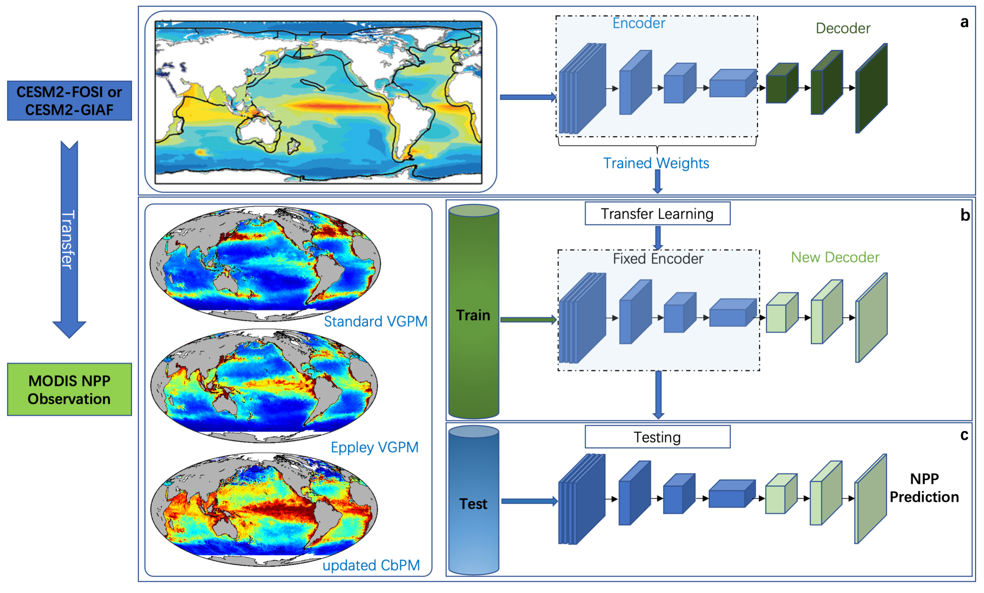
2.3. The Workflow of Transfer Learning
In this study, we apply transfer learning for NPPCast and UNet-family baselines. As illustrated in Figure 2, the workflow comprises three stages of transfer learning for the UNet family of models: pre-training, fine-tuning, and testing.
Figure 2.
The training stages of UNet-family and NPPCast. (a) Pre-training stage. (b) Transfer-learning/fine-tuning stage. (c) Testing stage.
Stage 1 (Pre-training): We use monthly CESM2 NPP from FOSI (1958–2020) and GIAF (1958–2018), both on the CESM2 nominal ocean grid (). As a scale reference, in latitude is ∼110 km at the equator, with zonal spacing decreasing poleward. Monthly NPP fields from CESM2–FOSI or CESM2–GIAF (36-month input, 36-month target; stride = 1 month) are used to train five architectures. For FOSI, data from January 1958 to December 2004 serve as the training set, with the 2005–2020 period held out for validation; for GIAF, the split is January 1958–December 2002 for training and January 2003–2018 for validation. Encoder–decoder CNNs (UNet, VNet, AttUNet, R2UNet) learn encoder weights and decoder weights , while NPPCast learns parameter .
Stage 2 (Fine-tuning): We adapt the models to satellite products (SVGPM, EVGPM, CbPM, and the mean of the three). All satellite fields are regridded to the same CESM2 ocean grid for consistency. We use matched sliding windows: 36 months input and 36 months target. For each satellite product, the first 10 years of the MODIS era (1998–2007) provide fine-tuning training windows. The remaining years (2008–2021) provide validation windows (targets ending in 2008–2021). This split is applied identically to SVGPM, EVGPM, CbPM, and MEAN.
Stage 3 (Testing): In the final stage, each fine-tuned model is evaluated on the held-out portion of the MODIS NPP datasets, generating predictions for those unseen samples. Table 1 summarizes the datasets used in this study.
Table 1.
Datasets employed in this study. All datasets were re-gridded to the native grid of CESM2 ocean component (a nominal horizontal resolution of ) to ensure spatial consistency between model simulations and observational products.
We evaluate leads from 1–36 months but focus interpretation on 12–36-month leads. Marine NPP exhibits demonstrable potential predictability on seasonal-to-multiannual windows (roughly 1–3 years) in many ocean regions, providing a clear scientific basis for emphasizing out-year skill. By contrast, sub-annual leads are often well approximated by persistence or climatology and add limited value for multi-season planning in our setting.
For UNet-family baselines, we initialize from pre-training, freeze the encoder, and update only the decoder. This is a standard regularization choice in noisy, small-to-moderate data regimes to preserve stable multi-scale spatial filters and avoid catastrophic forgetting. For NPPCast, we initialize all layers from pre-training and fine-tune end-to-end on each satellite product. This is because NPPCast has a temporal, region-specialized backbone without a deep spatial encoder/decoder split. End-to-end fine-tuning is the natural choice to adapt temporal embeddings and lead-dependent dynamics. Accordingly, fairness in this comparison hinges on the models’ effective capacity under noisy supervision and their architectural inductive biases, rather than on the raw count of trainable parameters.
Pre-training on CESM2 provides a long, globally complete, noise-reduced record that teaches the network canonical seasonality and low-frequency modes of NPP variability. Fine-tuning on satellite products then anchors the forecasts to observed amplitudes and regional patterns, correcting model-specific biases and sharpening coastal features. In short, climate-model data confer generality and physical consistency, while satellite products confer fidelity to observations.
2.4. Spatial Partitioning and Window Slicing
Given an input data cube (with T time steps and a spatial grid of size for a single variable, for simplicity), we define a binary mask indicating ocean vs. land at location . We apply this mask to filter out or zero out values in regions not of interest (e.g., land points when forecasting an oceanic variable), yielding a sparsified input. We then partition the remaining ocean domain into G disjoint, contiguous regional tiles on the grid. Each tile preserves local neighborhoods (no interleaving of distant cells) and contains approximately the same number of ocean points. Each region is treated as a collection of grid points (channels) that will be modeled together.
Formally, for region g we construct a multivariate time series:
which is the vector of values at time t for all locations u in . To prepare training samples, we employ a sliding window approach in time: at each timestep t, the model takes the past observations of that region as input and predicts the values for the next steps.
In other words, the input window for group g is
and the model learns to output , which approximates the ground truth future sequence . We denote the forecasting function for group g as
Each regional forecaster consumes the past months (three years) of data from its tile to produce -month forecasts. With contiguous regions on the CESM2 POP nominal ocean grid ( with land masked), a typical region covers about (roughly meridional by – zonal at mid–latitudes).
All G regional models operate in parallel on their respective sub-series, greatly reducing the complexity compared to a global model. Because each focuses on a smaller subset of correlated locations, it can more effectively capture local patterns without interference from distant regions, and it naturally preserves temporal causality (each model uses only historical data from its region).
Spatial partitioning: definition, rationale, and G-invariance. We partition the masked ocean grid into G disjoint, contiguous tiles so that each pixel’s local neighborhood remains within a single tile. Contiguity preserves geographic coherence and avoids non-physical mixing of distant provinces, while roughly equal tile sizes secure sufficient samples per region to stabilize the learning of seasonal phase and low-frequency variability. In NPPCast, this partition functions as a compute/batching device rather than a scientific hyperparameter: the regional forecaster applies the same architecture and per-pixel objective to each tile, and the final field is obtained by identity remap with a light per-pixel 1 × 1 affine fusion. Because the temporal cores are channel-separable with permutation-equivariant mixing, re-indexing or re-grouping channels does not change the hypothesis class or the per-pixel loss being minimized. Consequently, accuracy is invariant to G up to boundary effects, provided tiles are contiguous and wide enough to contain each pixel’s local neighborhood. In this study we use micro-regions to saturate an A40 (48 GB) GPU at ; different G values would alter memory layout and throughput but not the modeling assumptions. Full algorithmic details and a formal G-invariance argument are provided in the Appendix E.
2.5. Fusion of Regional Outputs
Once each regional model produces a forecast for its area, NPPCast recombines these outputs into the final spatiotemporal prediction. We first map each group’s predicted values back to their original spatial locations. In case of any overlap between regions or to account for global consistency, we introduce a 1 × 1 convolutional layer to fuse the multiple regional predictions into one coherent output field. This 1 × 1 convolution operates across the channel dimension (where each channel holds the contribution of one region at the same spatial location) and learns an optimal linear combination of the regional contributions. Mathematically, if denotes the predicted field (upscaled to the full map size, with zeros outside ) from model g at lead time h, the fused prediction is:
where is a learnable weight matrix (of the same dimension as , here implemented as shared parameters in the 1 × 1 convolution filter for channel g) and b is a bias term. In practice, the 1 × 1 convolutional fusion yields a smooth blending of regional outputs and corrects any systematic biases, resulting in the final predicted field . By construction, NPPCast’s framework can flexibly incorporate additional regions or masks, which ensures that each forecast is driven by appropriate local information, addressing the heterogeneity in spatiotemporal data.
2.6. Improved TimesNet for Regional Temporal Modeling
For modeling each regional time series, we build upon the TimesNet architecture [], which was originally proposed as a general backbone for time series analysis. TimesNet employs a novel TimesBlock that can adaptively capture multiple periodic patterns in a time series by transforming the 1D sequence into a 2D representation. We briefly recap this mechanism and then describe the specific modifications made for NPPCast.
2.6.1. Multi-Period 2D Transformation
Given an input sequence of length T (after an initial linear embedding layer to project the variables to a d-dimensional feature space), TimesBlock identifies dominant period lengths in the series via a frequency analysis. Let be the embedded input for a particular region and layer. We apply a period detection operator that returns a set of k significant periods (e.g., by locating peaks in the Fourier amplitude spectrum of ). For each period , the sequence is zero-padded to length (where ) and then reshaped into a 2D tensor . In this 2D “period-aligned” view, the horizontal axis indexes positions within one period ( time steps), and the vertical axis indexes different period cycles (total cycles covering the whole timeline). In this way, temporal variations that occur within a single period manifest as patterns along each row, while variations across periods (long-term trends or changes between cycles) appear down the columns. This 1D-to-2D reshaping makes it convenient to apply 2D convolution kernels to capture temporal dynamics on both short and long scales simultaneously. We then feed each into a shared multi-scale convolution module to extract feature maps . This module was originally designed based on the Inception architecture. In TimesNet, this module deploys parallel convolutions of different kernel sizes (e.g., , , ) to effectively capture multi-scale temporal variations in the 2D domain. After convolution, each output is reshaped back to 1D by undoing the period layout and truncating any padded points, yielding a processed sequence for that period hypothesis.
Finally, TimesBlock adaptively aggregates the k reconstructed sequences using weights that reflect the empirical strength of each detected period in the input series. Concretely, let denote the normalized amplitude associated with period (obtained from the frequency spectrum, e.g., via a softmax over the top-k period amplitudes), then the TimesBlock output is computed as a weighted sum:
where represents the attention weight for period . Through this multi-period detection and fusion mechanism, TimesNet effectively unravels complex temporal patterns into several simpler components and models them jointly, which has been shown to achieve state-of-the-art accuracy on various forecasting benchmarks.
2.6.2. TimesNet Modifications in NPPCast
We adapt the TimesNet architecture to better suit the regional forecasting setting and further improve its efficiency. First, instead of treating each variable (grid point) independently or all together, we preserve local spatial correlations by grouping neighboring points into one multivariate series (as described in the framework). This can be seen as a form of patch-wise channel grouping, which ensures that highly related channels are modeled within the same TimesNet. Such an approach retains inter-variable dependencies within each region while still avoiding a fully channel-dependent model on the entire grid, striking a balance between modeling complexity and specialization. Second, we refine the convolutional module inside TimesBlock to reduce the parameter count and avoid overfitting for each regional model. In the original TimesNet, the multi-scale inception block employs standard convolutional filters of sizes , , etc., applied to the 2D tensor.
In NPPCast, we implement these convolutions using a depthwise separable convolution strategy. Specifically, for each kernel size, we perform a depthwise convolution (DWConv) that operates on each feature channel independently across the spatial domain, followed by a pointwise convolution (PWConv) that mixes information across channels. This DW + PW combination realizes the same receptive field as a standard convolution but with far fewer parameters, since the depthwise stage has d separate small kernels (one per channel) and the pointwise stage has kernels to linearly combine the d channels. By sharing the multi-scale DWConv-PWConv module across all k period-based tensors (as in the original design), our TimesBlock variant remains size-invariant with respect to k and is highly parameter-efficient. Empirically, this modification helps prevent the regional models (which are relatively lightweight) from over-parametrization, without sacrificing their ability to capture multi-scale temporal features. In addition, since NPPCast trains separate TimesNet models for each region, these models can be run in parallel and specialized to local patterns, leading to faster inference and better overall performance when compared to a single large model covering the entire domain.
For each region, we use a linear embedding of dimension and a stack of 3 TimesBlocks; each TimesBlock extracts up to dominant periods via parallel 1-D convolutions with kernel lengths (Inception-style). This configuration yields approximately M parameters per region; with regions the total is M parameters (excluding the light fusion layer). Models are optimized with Adam, using standard weight decay of ; we do not use layer-wise learning-rate decay or dropout.
2.7. Metrics
We assess model performance using a suite of complementary error and similarity metrics, as defined in Table 2. Specifically, root mean square error (RMSE) and mean absolute error (MAE) quantify the average magnitude of forecast errors; anomaly correlation coefficient (ACC) evaluates linear agreement between predictions and observations; the Nash–Sutcliffe efficiency (NSE) measures relative predictive skill; and the Structural Similarity Index (SSIM) captures spatial fidelity of the forecast fields. Detailed formulae and usage notes are provided in the table.
Table 2.
Error and similarity metrics used in this study.
3. Results
3.1. Temporal Decay of Predictive Skill
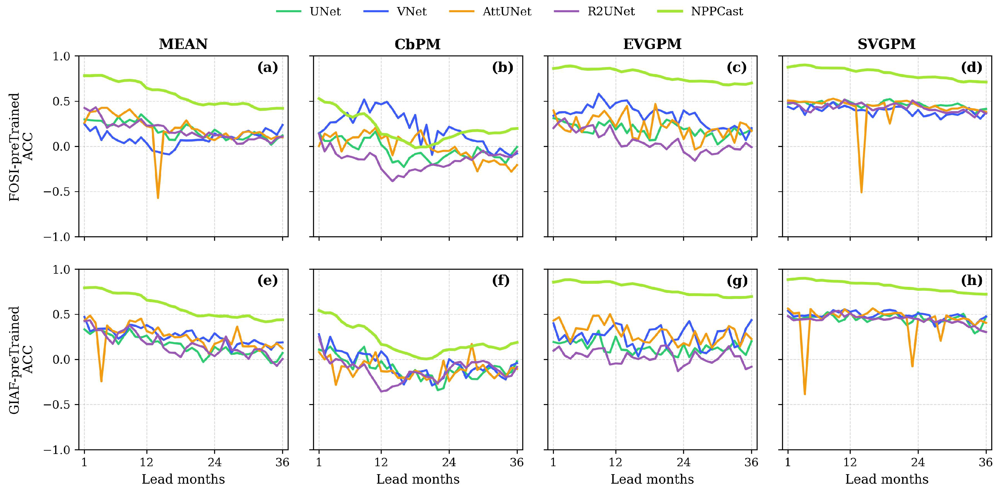
Figure 3 shows the lead-time decay of ACC for each model and dataset under both CESM2-FOSI and CESM2-GIAF pretraining. Across MEAN, EVGPM, and SVGPM, NPPCast starts with the highest ACC at short leads (typically ∼0.7–0.9 at L = 1) and retains a clear margin through L = 36, while the UNet, VNet, and R2UNet curves decay more steeply. Under GIAF pre-training this ranking persists for all four products, including CbPM. The one notable exception is CbPM with FOSI pre-training: here, the separation between models is smaller, with all methods occupying a midrange band and NPPCast’s advantage less pronounced than in the other panels. AttUNet shows the largest volatility, with intermittent troughs (including occasional dips toward or below zero ACC) at intermediate leads in several products, whereas UNet, VNet, and R2UNet decay more smoothly. Overall, aside from the FOSI–CbPM case, NPPCast consistently maintains the highest ACC and the slowest lead-time degradation across both pre-training scenes.
Figure 3.
Lead-time evolution of ACC for UNet, VNet, AttUNet, R2UNet, and NPPCast under CESM2–FOSI (top row, (a–d)) and CESM2–GIAF (bottom row, (e–h)) pre-training across four MODIS products. In most settings (MEAN, EVGPM, SVGPM, and CbPM under GIAF), NPPCast exhibits the slowest decay and maintains clearly higher ACC at long leads than the UNet-family baselines; the contrast is appreciably weaker for CbPM with FOSI pre-training, where all methods cluster and the gap narrows.
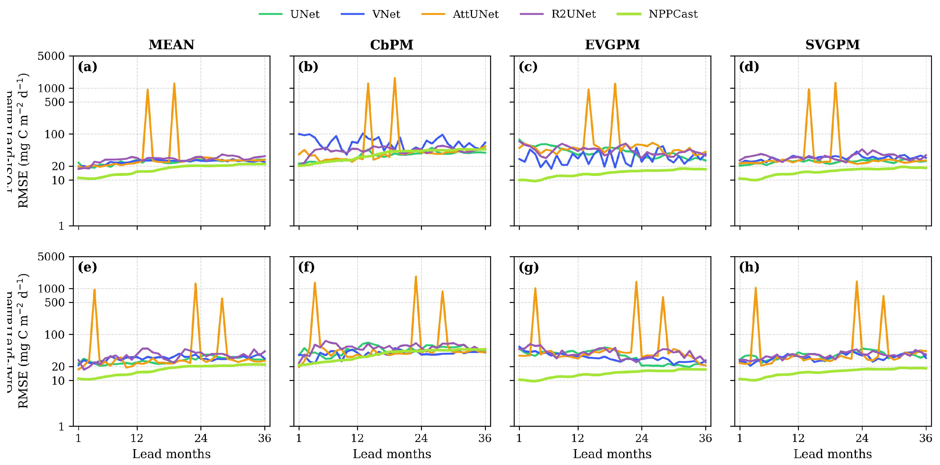
The RMSE decay curves in Figure 4 exhibit the complementary pattern: NPPCast generally maintains the lowest and increases only gradually with lead, whereas UNet, VNet, and R2UNet show larger and more variable growth. In the MEAN product, for example, NPPCast’s curve remains comparatively flat over 1–36 months, while AttUNet exhibits intermittent mid-lead spikes (e.g., around 14 and 19 months). (These spikes are tied to occasional failures of the attention gating that produce implausible negative predictions and heavy-tailed errors, which motivates the scaling; diagnostic evidence and discussion are provided in Appendix C). The same ranking holds for EVGPM and SVGPM under both CESM2–FOSI and CESM2–GIAF pre-training. The CbPM product is a partial exception: all models incur higher errors and NPPCast’s advantage narrows, with a few lead months where the best UNet-family baseline matches or slightly outperforms NPPCast; nonetheless, NPPCast retains the lowest average RMSE across the full horizon. Altogether, the curves indicate that NPPCast’s error growth is more gradual and stable, while AttUNet is prone to large, sporadic surges and the other UNet-based baselines drift upward more quickly with lead.
Figure 4.
Lead-time evolution of for UNet, VNet, AttUNet, R2UNet, and NPPCast. Rows show CESM2–FOSI (top, (a–d)) and CESM2–GIAF (bottom, (e–h)) pre-training; columns correspond to the four MODIS NPP products. Overall, NPPCast exhibits the slowest error growth and the lowest across most leads—clearly so for MEAN, EVGPM, and SVGPM. For CbPM, the separation is weaker and NPPCast’s curve intersects the best UNet-family baseline at a few leads under both pre-training scenes. Note: RMSE values are shown on a scale with tick labels converted to actual values for clarity.
3.2. Spatial Pattern Fidelity at Different Scale Leads
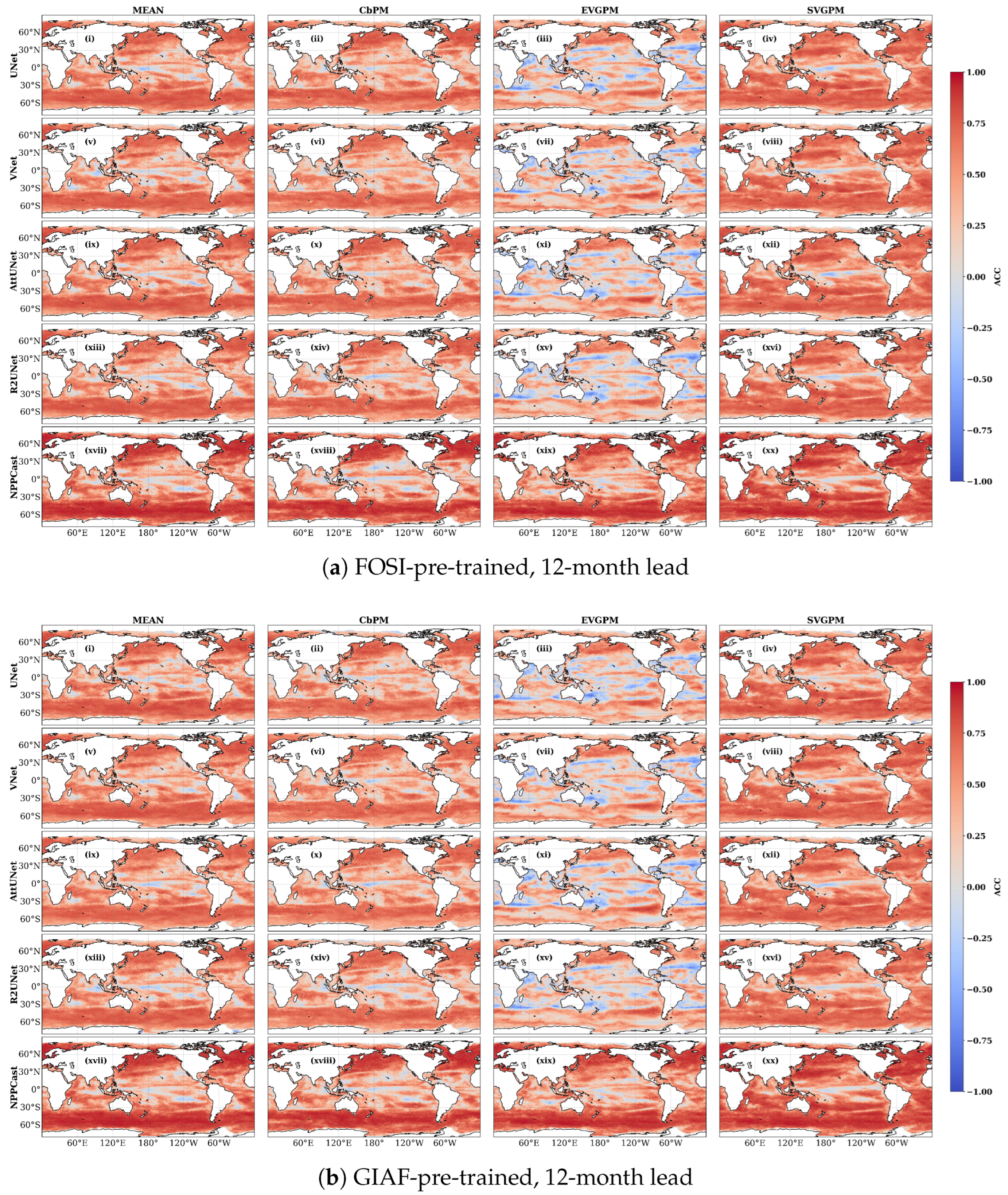
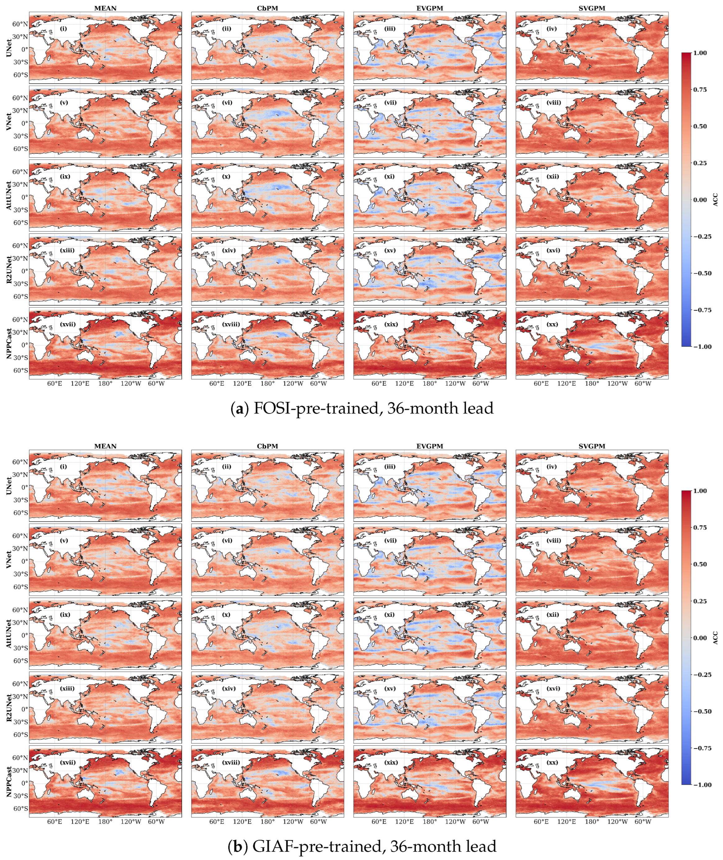
The spatial distribution of ACC reveals that both NPPCast and UNet-family models capture broad-scale climate patterns at 12-month lead, but with clear latitude- and region-dependent differences. In all cases, the region between 30°N and 30°S exhibits low ACC values, suggesting limited predictive skill in the tropics, whereas extratropical ocean basins exhibit the highest ACC.
At a 12-month lead (Figure 5), NPPCast yields systematically higher ACC than the UNet baselines across most mid-latitude regions. For example, over the North Atlantic and adjacent Pacific (roughly 30–60°N) and over the Southern Ocean (30–60°S), NPPCast retains warm shades of ACC, whereas the UNet variants show more muted values. Conversely, along the Equator (especially 0–30°N and 0–30°S in the central Pacific), ACC is near zero for all models in both the FOSI and GIAF cases. Thus, at the 1-year lead, the main difference in spatial fidelity is that NPPCast preserves coherent basin-scale anomaly structures—particularly the mid-latitude bands in the North Atlantic and Southern Ocean—more faithfully than the UNet family in both pre-training scenes. For brevity, the 24-month-lead maps display the same latitude-dependent contrasts as the 12-month case with a broadly reduced amplitude; the corresponding panels and a short commentary are provided in Appendix A.
Figure 5.
Spatial distribution of ACC at a 12-month lead time for the two pre-training scenarios. In every sub-panel the rows compare the five networks (UNet (i–iv), VNet (v–viii), AttUNet (ix–xii), R2UNet (xiii–xvi), NPPCast (xvii–xx)), and the columns compare the four MODIS NPP products. Warm hues (red) denote positive skill, cool hues (blue) negative skill. NPPCast (bottom row) already exhibits the highest and most geographically consistent skill across both pre-training datasets, especially in the oligotrophic gyres and high-latitude bloom regions.
In the 36-month FOSI-pretrained map (Figure 6), NPPCast shows faint but positive ACC (light shading) over the southern Pacific/Indian basins and parts of the North Atlantic, whereas the equatorial regions remain at low values. The GIAF-pretrained 36-month map likewise exhibits residual skill in similar zones, with NPPCast’s ACC modestly above zero at mid- to high-latitudes. In summary, NPPCast maintains spatial fidelity substantially longer than the UNet baselines: even at a three-year lead it preserves the imprint of dominant large-scale modes in mid-latitudes and Southern Ocean, whereas the UNet-family predictions have decorrelated from the true patterns. This latitudinal/regional contrast (persistent mid-latitude skill versus tropic collapse) is evident in both the FOSI and GIAF pre-training scenarios, although the exact zonal features differ slightly between datasets (for instance, GIAF pre-training yields relatively higher ACC in the Indo-Pacific sector at 1-year, whereas FOSI emphasizes the Atlantic sector). Overall, these ACC maps demonstrate that NPPCast’s multi-year forecasts maintain realistic spatial fidelity substantially longer, preserving the imprint of large-scale modes well beyond the point where traditional UNet-based approaches lose coherence. In both FOSI and GIAF cases, NPPCast’s advantage grows with lead, highlighting a much slower degradation of spatial skill compared to the UNet-family models.
Figure 6.
Spatial distribution of ACC at a 36-month lead time (UNet (i–iv), VNet (v–viii), AttUNet (ix–xii), R2UNet (xiii–xvi), NPPCast (xvii–xx)). Positive skill has largely vanished for all UNet variants, whereas NPPCast still yields statistically significant pattern correlation in the North Atlantic, western Indo-Pacific, and parts of the Southern Ocean in both pre-training scenes. The consistency across independent climate forcings confirms that NPPCast’s superior long-range pattern fidelity does not hinge on the choice of the pre-training dataset.
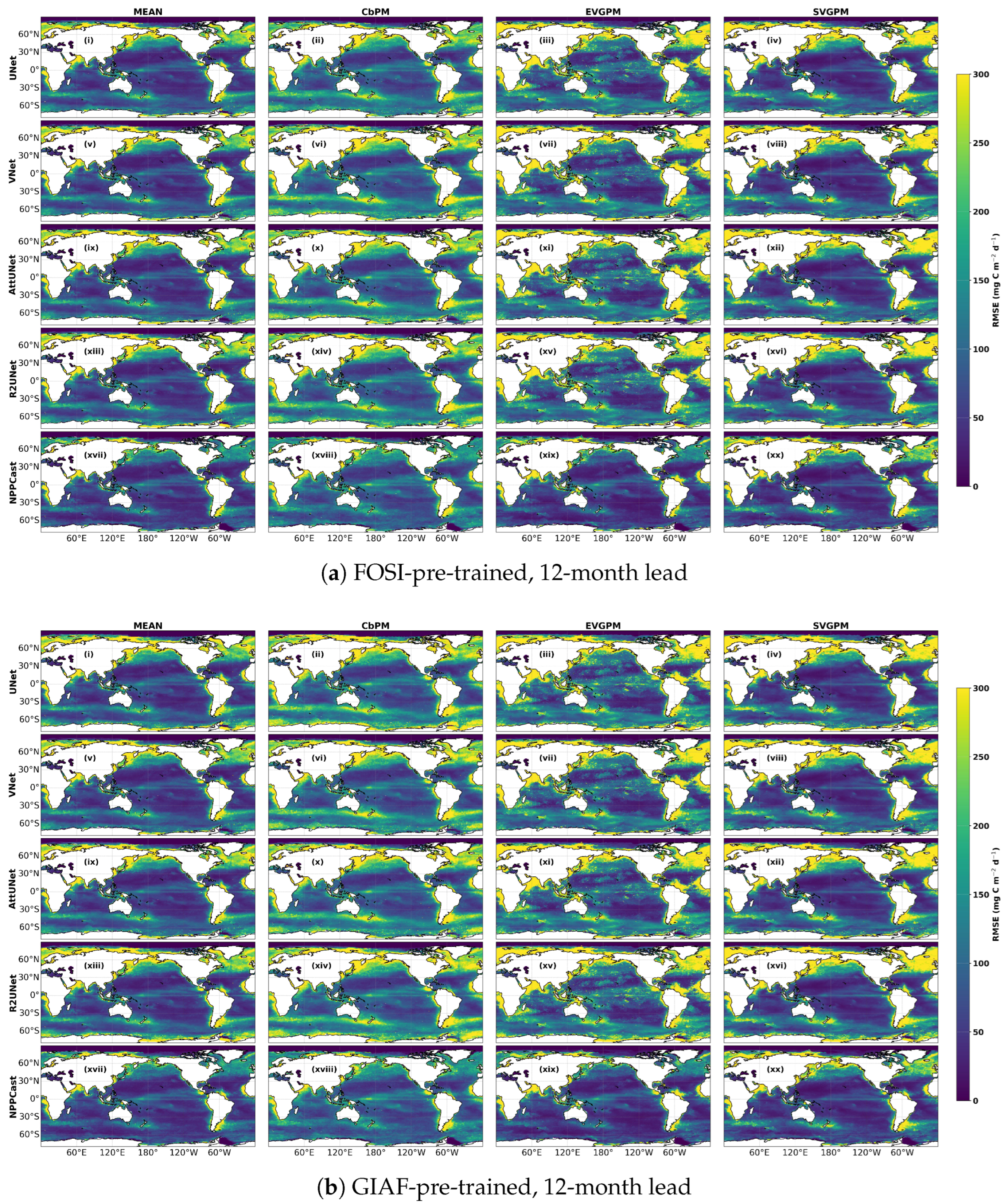
We further analyzed the spatial distribution of RMSE at different prediction lead times. The results show that, at a 12-month lead time (Figure 7), all models exhibit similar spatial error patterns, with larger errors generally occurring in high-latitude regions (the North Atlantic, the North Pacific, and the Southern Ocean), coastal areas, and the extension regions of the western boundary current, while smaller errors are found in the subtropical oligotrophic gyres. Compared with the CbPM products, the other products exhibit relatively larger errors in high-latitude and coastal ocean regions. In contrast, NPPCast consistently achieves lower RMSE than the UNet family across most ocean basins, with particularly pronounced improvements in the Southern Ocean and the high-latitude regions of the Northern Hemisphere. The results under the FOSI and GIAF cases differ only slightly, and their overall spatial patterns remain largely consistent.
Figure 7.
Spatial distribution of RMSE at a 12-month lead time for the two pre-training scenarios (UNet (i–iv), VNet (v–viii), AttUNet (ix–xii), R2UNet (xiii–xvi), NPPCast (xvii–xx)).
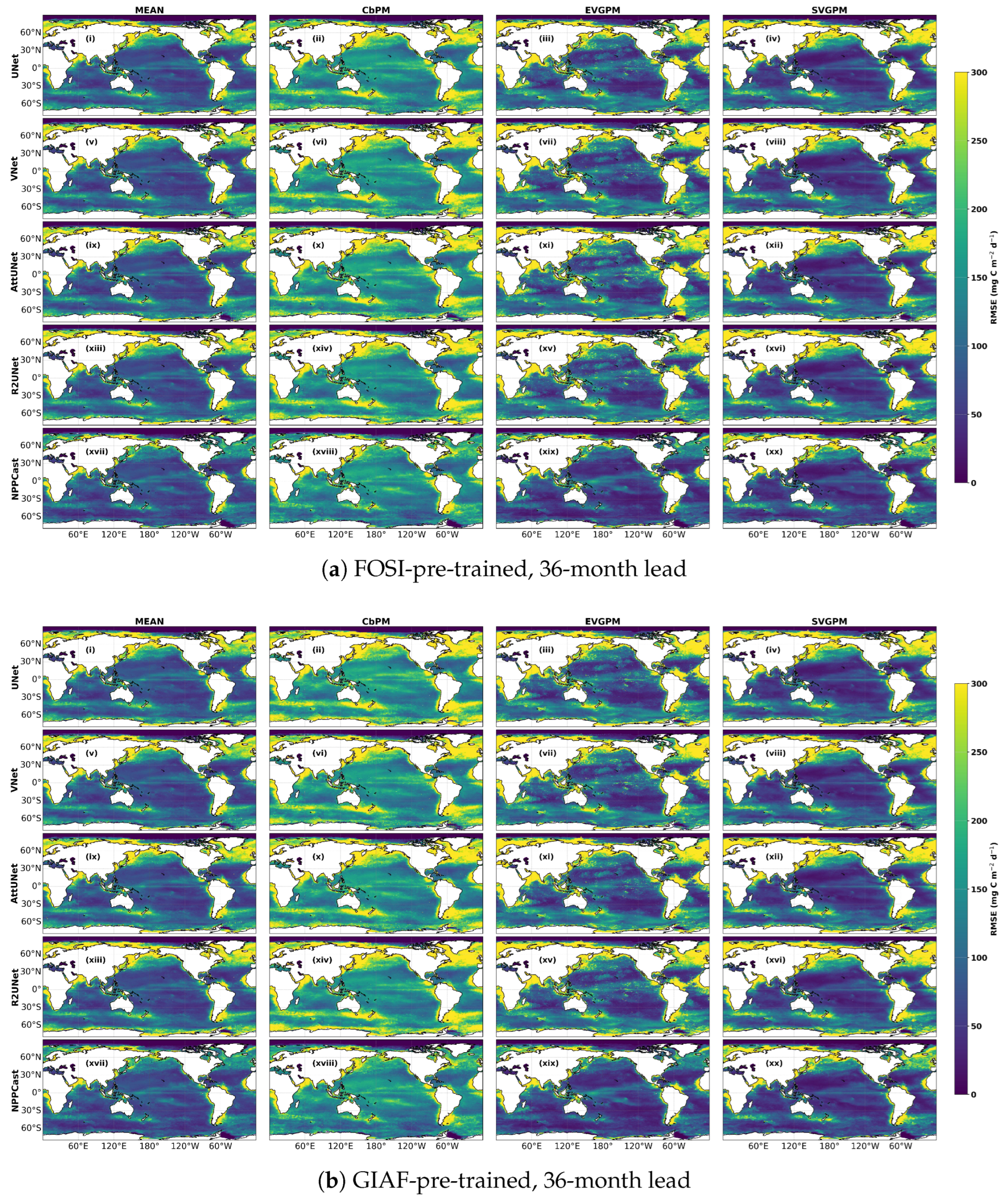
At 36-month lead time (Figure 8), the RMSE increases compared to the 12-month lead, although the spatial distribution pattern remains consistent. This indicates a gradual decline in the predictability of NPP with longer lead times. Nevertheless, NPPCast maintains relatively low error levels across most ocean regions and continues to exhibit clear and stable spatial error patterns even at the 36-month lead time. Overall, at both the one-year and three-year leads, NPPCast consistently demonstrates the highest spatial coherence and the lowest global error magnitude among all models, highlighting its robustness and superior generalization capability in long-lead marine productivity prediction. The RMSE for 24-month lead time can be found in Appendix A.
Figure 8.
Spatial distribution of RMSE at a 36-month lead time for the two pre-training scenarios (UNet (i–iv), VNet (v–viii), AttUNet (ix–xii), R2UNet (xiii–xvi), NPPCast (xvii–xx)).
3.3. Quantitative Performance Metrics
Quantitative metrics show that NPPCast delivers the best monthly global NPP forecasts across products and under both pre-training scenes, with consistently lower errors (RMSE, MAE) and higher skill scores (ACC, NSE, SSIM) than the UNet-family baselines, except for CbPM under FOSI where RMSE is slightly higher and ACC ties the best baseline (Table 3).
Table 3.
Performance metrics (RMSE (unit: mg C ), MAE (unit: mg C ), ACC, NSE, SSIM) for five forecasting models under two pre-training scenarios (FOSI-PreTrained and GIAF-PreTrained) across four MODIS NPP products (MEAN, CbPM, EVGPM, SVGPM). Metrics pool all lead months (1–36), all samples and grid cells. Lower RMSE/MAE and higher ACC/NSE/SSIM are better. Best in each product–scenario–metric is bold; second best is underlined.
For the MEAN product, NPPCast attains the lowest RMSE and MAE and the highest ACC, NSE, and SSIM in both scenes. Under FOSI-PreTrained, NPPCast achieves RMSE = 17.22 versus the next best (UNet) and ACC = 0.57 versus the next best (AttUNet). Under GIAF-PreTrained, NPPCast again yields RMSE = 17.22 versus (UNet) and ACC = 0.58 versus (VNet). NSE is positive only for NPPCast ( in both scenes), whereas all baselines are negative; SSIM reaches for NPPCast versus for baselines.
For EVGPM, NPPCast shows the largest gains. Under FOSI-PreTrained, RMSE drops to compared with the best baseline (VNet), and ACC reaches versus (VNet). Under GIAF-PreTrained, NPPCast retains RMSE versus (VNet) and ACC versus (AttUNet). Importantly, NPPCast is the only model with positive NSE on EVGPM ( FOSI; GIAF), and it has the highest SSIM ().
For SVGPM, NPPCast again leads across metrics. Under FOSI-PreTrained, RMSE vs. (UNet) and ACC vs. (UNet). Under GIAF-PreTrained, RMSE vs. (VNet) and ACC vs. (VNet). NPPCast is the only method with positive NSE ( FOSI; GIAF) and reaches SSIM .
The only exception occurs for CbPM/FOSI-PreTrained: NPPCast’s RMSE is slightly higher than the best baseline (36.31 vs. 34.1 for UNet) and its ACC ties the best baseline (both ). Nevertheless, NPPCast still attains the highest SSIM (). Under CbPM/GIAF-PreTrained, NPPCast regains a small but clear lead: RMSE vs. (VNet) and ACC vs. (VNet).
A concise view of the gains relative to the best UNet-family baseline is given by Table 4. For ACC, NPPCast’s advantage ranges from a tie on CbPM/FOSI () to on EVGPM/GIAF-PreTrained (and on EVGPM/FOSI-PreTrained). For RMSE, the relative reduction spans from a slight deficit on CbPM/FOSI-PreTrained (, i.e., NPPCast marginally worse) to very large improvements on EVGPM (about 55.6–55.8%) and SVGPM (39.0–52.7%), with substantial gains also on MEAN ( FOSI-PreTrained; GIAF-PreTrained). These deltas corroborate that NPPCast’s largest advantages appear on EVGPM and SVGPM, while CbPM/FOSI-PreTrained is the only case where NPPCast does not reduce RMSE relative to the best baseline.
Table 4.
NPPCast vs. the best UNet-family baseline: ACC and RMSE(%).
To gauge how strongly each network depends on the dynamical context seen during pre-training, we quantify the percentage change in every skill metric when the pre-training data are switched from CESM2–FOSI outputs to CESM2–GIAF outputs:
Negative values denote deterioration in skill (larger errors or lower correlations) while positive values signify improvement.
Across all four MODIS NPP products (Table 5), the UNet family shows substantial scene sensitivity, with large percentage changes in accuracy and error metrics when pre-trained on different dynamical regimes. For MEAN, UNet and its variants (VNet, AttUNet, and R2UNet) display shifts up to in ACC and in RMSE. In contrast, NPPCast remains nearly invariant (ACC , RMSE ), indicating strong robustness.
Table 5.
Percentage change ( %) from FOSI- to GIAF-pretraining for five models across four MODIS NPP products. Columns are ACC, RMSE, MAE, NSE, and SSIM. Within each product and metric, the smallest absolute change is in bold and the second smallest is underlined.
For CbPM, UNet and AttUNet exhibit particularly high volatility (RMSE , ACC ), whereas VNet reduces error magnitudes but loses correlation. NPPCast varies by less than . Similar trends occur for EVGPM and SVGPM: UNet-based models exhibit pronounced sensitivity, while NPPCast changes remain minimal ( for most metrics).
3.4. Prediction vs. Observation Scatter
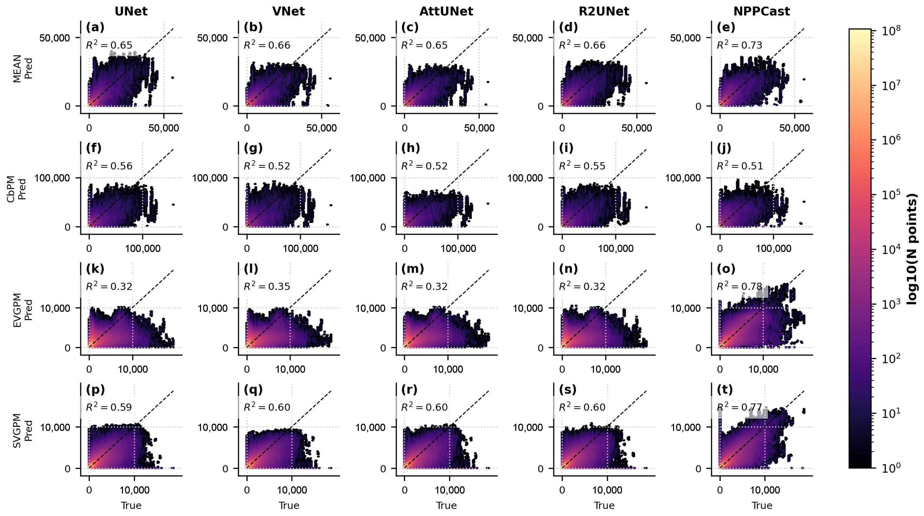
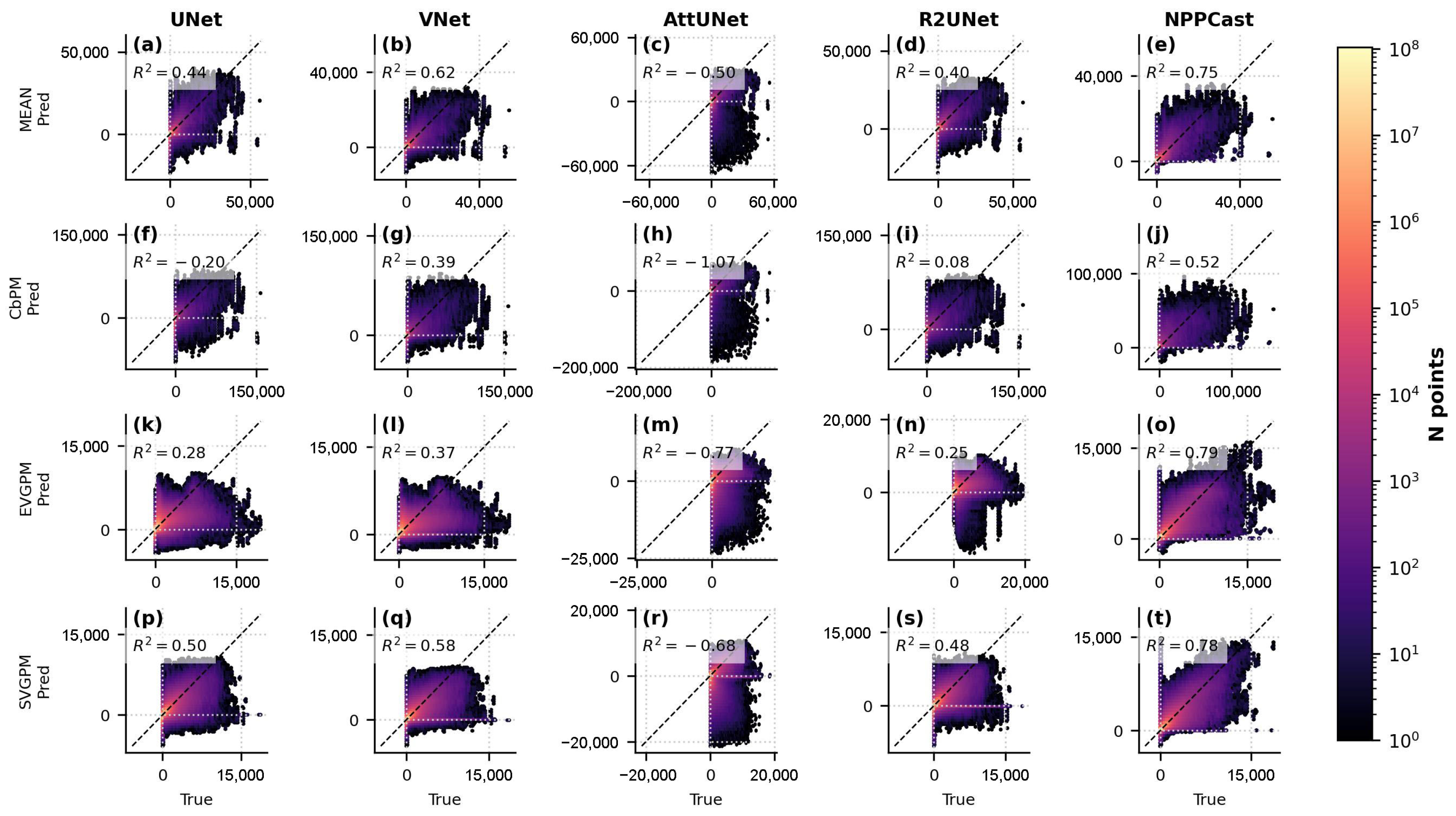
The agreement between predicted and observed NPP is illustrated in 1:1 scatter plots (Figure 9 for FOSI-pretrained models and Figure 10 for GIAF-pretrained). In these plots, NPPCast’s predictions cluster tightly along the 1:1 line across the full NPP range, indicating accurate reproduction of both low- and high- productivity regimes with minimal bias. The NPPCast point cloud is compact, with a near-unity slope and high (consistent with ACC ), demonstrating that it captures variance of the observations extremely well. By contrast, the baseline models exhibit more scatter around the identity line. For instance, at higher NPP values (e.g., in productive upwelling zones), the baseline model predictions tend to underestimate the observed NPP, as evidenced by points falling below the 1:1 line. NPPCast significantly mitigates this underestimation. Likewise, at very low NPP levels (oligotrophic regions), some baselines show slight positive biases (points above the line), whereas NPPCast remains well-aligned. The similarity of NPPCast’s scatter distribution between the FOSI and GIAF cases is also noteworthy: there is no visible degradation or change in bias when switching pre-training dataset. This consistency implies that NPPCast not only achieves superior aggregate error metrics, but also reliably reproduces the full range of NPP values and their spatiotemporal variability, making it a robust tool for both average conditions and extreme events.
Figure 9.
Predicted vs. observed NPP scatter density for FOSI-pretrained models (unit: mg C ). Each subplot corresponds to one CNN model (columns: UNet, VNet, AttUNet, R2UNet, NPPCast) and one MODIS-derived dataset (rows: MEAN (a–e), CbPM (f–j), EVGPM (k–o), SVGPM (p–t)). The color scale indicates point density in log space; the dashed line is the 1:1 identity. The coefficient of determination (upper-left of each panel) quantifies the tightness of the prediction–observation relationship. NPPCast (rightmost column) exhibits the highest (0.49–0.79 across datasets) and the least scatter around the 1:1 line, demonstrating superior fidelity in reproducing both low and high NPP values compared to the four CNN baselines, whose clouds are more dispersed and deviate more from the diagonal. See Appendix D for the explanation of negative R2 values.
Figure 10.
Predicted vs. observed NPP scatter density for GIAF-pretrained models. Layout as in Figure 9 (unit: mg C m−2 d−1) (rows: MEAN (a–e), CbPM (f–j), EVGPM (k–o), SVGPM (p–t)). Following GIAF pre-training, all models show modest shifts in bias and scatter, but NPPCast (rightmost column) maintains the highest R2 (0.52–0.79) and the most concentrated point distributions along the identity line. In contrast, the four CNN baselines display more pronounced off-diagonal spread—particularly at high NPP values—indicating that NPPCast’s pointwise agreement with observations is both tighter and more robust to changes in pre-training data.
3.5. Latitudinal Error Distribution
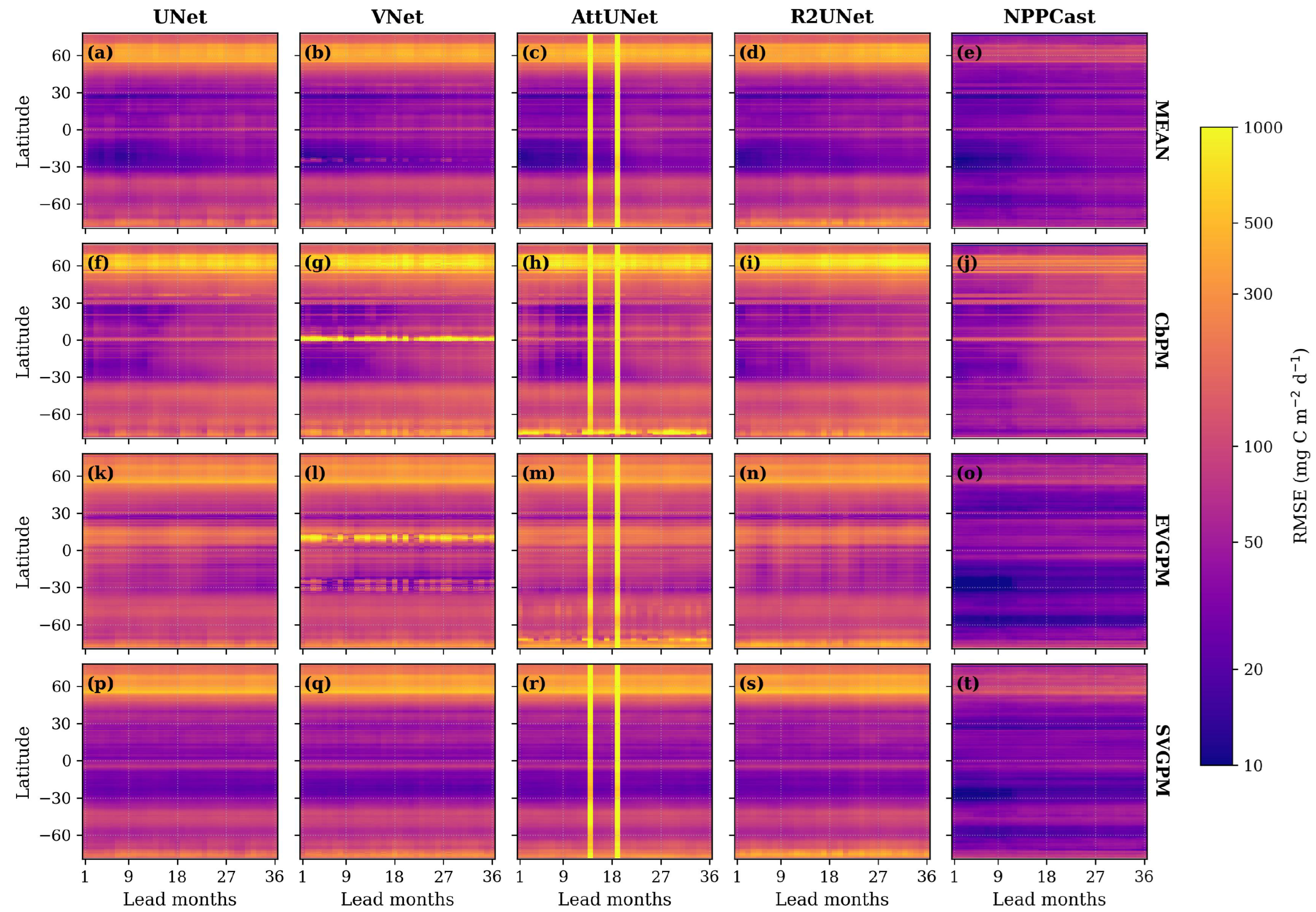
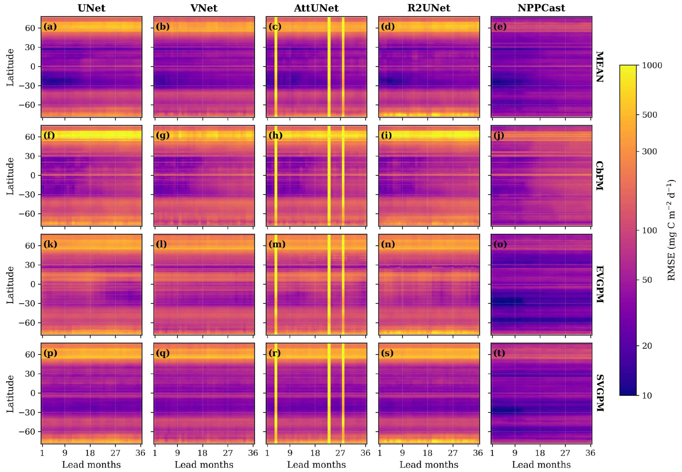
Latitude–lead Hovmöller plots of RMSE (mg C ; Figure 11 and Figure 12) for all five models under both FOSI- and GIAF-pretraining reveal systematic, latitude-dependent errors. Large errors concentrate in the equatorial band (∼10°S–10°N) and in mid-latitude upwelling regions (45°–60°N), consistent with known high-variability zones. Across nearly all latitudes and leads, NPPCast maintains the lowest RMSE, with its advantage most pronounced in these high-variance belts.
Figure 11.
Lead–latitude evolution for FOSI-pre-trained models. Each panel shows the latitude–lead Hovmöller diagram of RMSE (mg C ) between predicted and observed NPP. Columns correspond to the five models (UNet, VNet, AttUNet, R2UNet, NPPCast); rows correspond to the four MODIS-derived NPP products (MEAN (a–e), CbPM (f–j), EVGPM (k–o), SVGPM (p–t)). Warm colours denote large errors, cool colours small errors. Across all products, NPPCast (rightmost column) maintains the lowest RMSE throughout the 1–36-month forecast horizon, with minimal latitudinal striping, whereas the four CNN baselines exhibit pronounced error bands—especially at high latitudes and in the equatorial belt—that intensify with lead time. Note: RMSE values are shown on a scale with tick labels converted to actual values for clarity.
Figure 12.
Same as Figure 11 but for GIAF-pre-trained models. The error structure of NPPCast remains essentially unchanged, confirming its robustness to the choice of pre-training data. By contrast, several baselines (notably VNet and AttUNet) show a systematic reduction of equatorial and northern-subtropical errors after GIAF pre-training, evidencing their greater dependence on the training scene (MEAN (a–e), CbPM (f–j), EVGPM (k–o), SVGPM (p–t)). Despite these improvements, NPPCast still outperforms all baselines across latitudes and lead times.
In tropical latitudes around the equator (approximately 10°S–10°N), encompassing the equatorial divergence regions in the Pacific and Atlantic, NPPCast’s forecast errors are significantly lower than those of the UNet-based baselines. For example, in the equatorial Pacific, where strong interannual variability in NPP is driven by ENSO cycles, baseline models show sharp RMSE peaks, indicating large errors in predicting the timing and magnitude of El Niño/La Niña-related fluctuations. NPPCast considerably reduces these equatorial error peaks. At a 12-month lead, its RMSE in the equatorial band is about 15–20% smaller than the closest baseline, and this advantage persists (and even grows) at longer leads. By 36 months, the baselines show a band of elevated error spanning the equator (a “stripe” of red in the RMSE Hovmöller diagram), while NPPCast’s errors, though higher than at shorter leads, remain markedly lower. This behavior indicates that NPPCast retains skill for equatorial NPP fluctuations by maintaining a more consistent phase and amplitude of the seasonal–interannual cycle through lead time, without relying on any explicit multivariate mechanism.
In contrast, all models perform relatively well in the subtropical gyre regions, where low mean NPP and year-round stability prevail. As expected, the absolute errors are lower there for every model, since variability is minimal. NPPCast still yields the smallest errors in these low-variability zones, though the margin over baselines is narrower than in the more dynamic regions. This is because even a simple model can predict the persistently low productivity of gyres reasonably well, often by approximating climatology. Nevertheless, NPPCast’s slight edge in the gyres suggests it may be capturing subtle fluctuations, such as those from decadal oscillations or eddy-driven nutrient pulses, a bit more accurately than the baselines, contributing to its overall skill. (AttUNet displays two striking artifacts that are largely absent from other UNet baselines and NPPCast. A detailed diagnosis attributing this behavior is also provided in Appendix C).
3.6. Evaluating Differences in NPP Prediction Skill Between CESM2-SMYLE and NPPCast
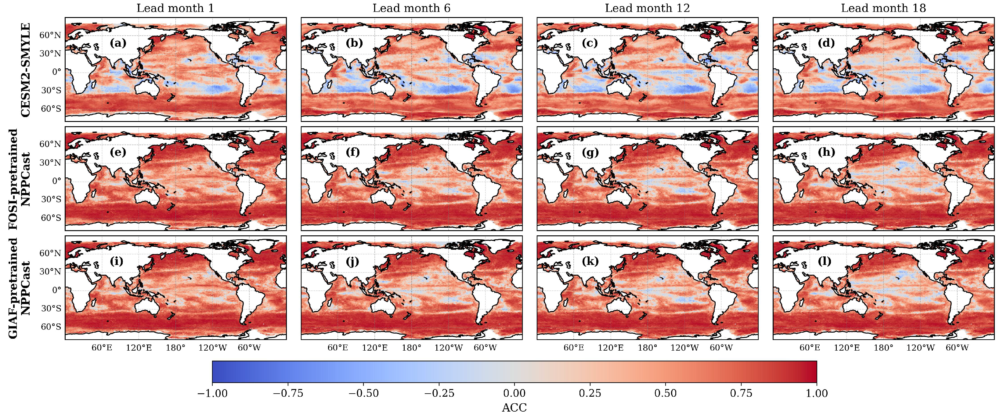
To evaluate the differences in predictive skill between Earth system model and the machine learning-based NPPCast model for NPP, we compared the ACC of forecasts from CESM2-SMYLE and two pretrained versions of NPPCast across different lead times (Figure 13). At a 1-month lead, CESM2-SMYLE exhibits moderate predictive skill (ACC > 0.5) in mid- and high-latitude regions such as the Southern Ocean and the North Atlantic. However, its performance is considerably weaker in mid- to low-latitude regions, particularly in the South Pacific and South Indian Ocean, where negative correlations occur in some areas. The FOSI- and GIAF-pretrained NPPCast models capture broader areas of positive correlation and higher predictive skill. It should be noted that this comparison is illustrative only, intended to highlight qualitative spatial–temporal differences rather than to establish a strict quantitative benchmark.
Figure 13.
Spatial distribution of ACC for NPP forecasts from CESM2-SMYLE. (a–d), FOSI-pretrained NPPCast (e–h), and GIAF-pretrained NPPCast (i–l) models at lead months 1, 6, 12, and 18.
As lead time increases to 6, 12, and 18 months, the skill of CESM2-SMYLE declines substantially, especially in the tropics, indicating limited temporal prediction. Meanwhile, the NPPCast models maintain robust correlation throughout the entire forecast horizon, continuing to exhibit significantly positive ACC even at 12- and 18-month leads, thereby reflecting stronger forecast persistence and extended predictive capability. These results suggest that when machine learning models are pretrained using long-term forced simulations such as CESM2-FOSI or CESM2-GIAF, the prediction of NPP can be substantially improved, potentially addressing key limitations of existing mechanistic models in biogeochemistry forecasting. Additional comparative results are provided in Appendix B.
4. Discussion
4.1. Drivers of Prediction Skill
4.1.1. Evolution of Prediction Skill with Initialization Time and Lead Time
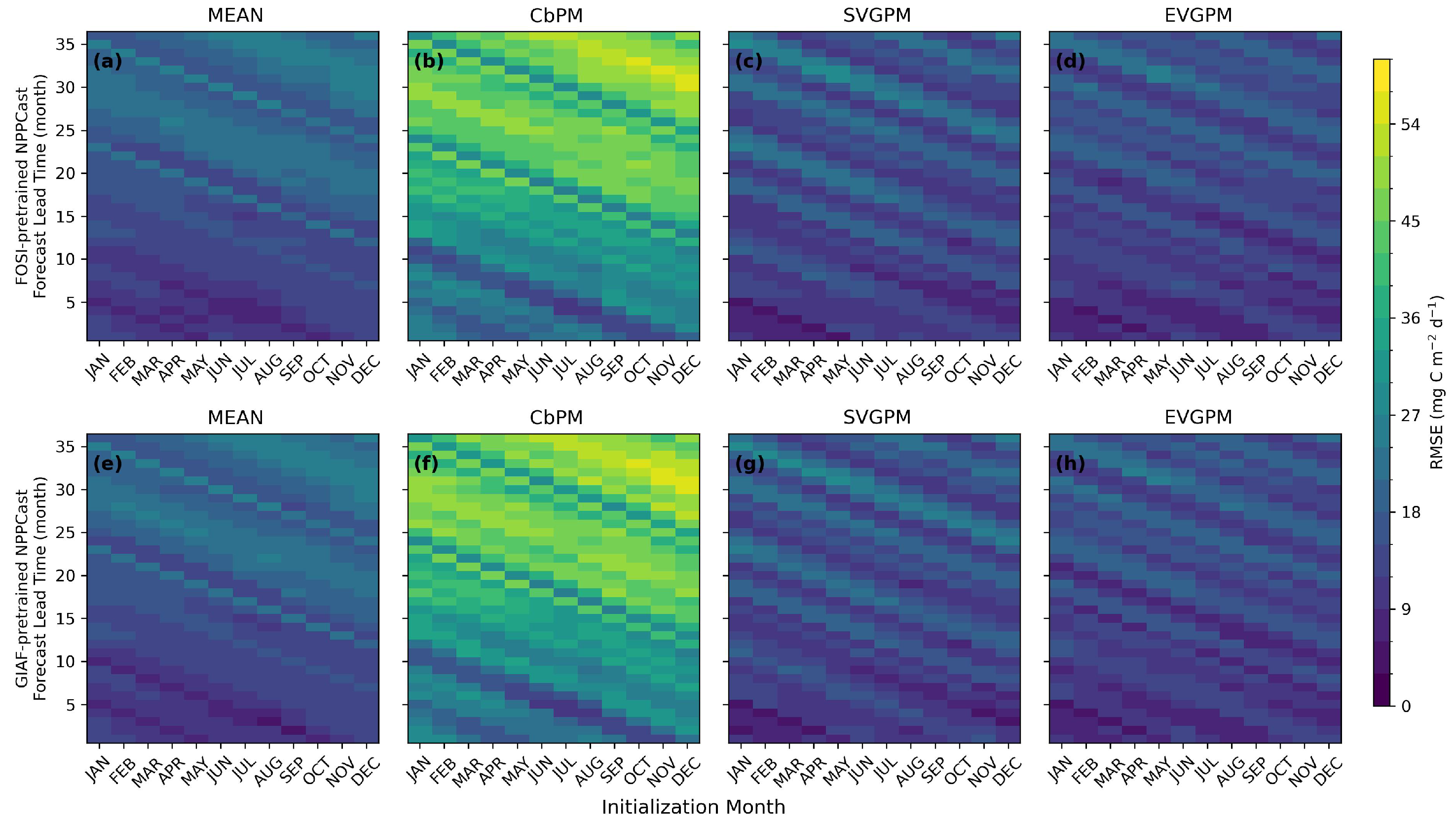
As shown in Figure 14, the RMSE of all models is strongly influenced by initialization month. Forecasts initialized in spring (March–May) and autumn (September–November) tend to exhibit lower RMSE, particularly when predicting NPP variability during the corresponding seasons, indicating higher prediction accuracy. In contrast, summer (June–August) and winter (December to February of the following year) initializations generally yield higher RMSE and reduced skill. All models show a consistent increase in RMSE with lead time, reflecting the expected decay of prediction skill over time. In addition, diagonal RMSE bands extending from the upper left to the lower right of each panel are evident, indicating alternating periods of error amplification and reduction associated with the seasonal cycle. These diagonal structures suggest that RMSE is primarily controlled by the target month/season rather than by the initialization month or lead time. For instance, when the prediction target is October, different combinations of initialization months and lead times that correspond to the same target month (i.e., forecasts targeting October) tend to exhibit similar error magnitudes. This consistency in error levels results in the formation of the diagonal patterns observed in Figure 14. Similar phenomena have also been reported in other studies, suggesting that this feature is not an isolated case but rather reflects a general pattern of seasonal predictability variations in the climate system [,]. This variation in seasonal predictability is responsible for the sensitivity of forecast errors to the seasonal background conditions, highlighting a strong coupling between the forecast initialization time and the biological seasonal dynamics of the ocean. Since this study employs a single-variable prediction approach without incorporating additional physical or biogeochemical variables, it is currently not possible to provide a detailed mechanistic interpretation. Future work will consider introducing these relevant variables to further investigate the underlying mechanisms.
Figure 14.
RMSE of NPP prediction skill as a function of initialization month and forecast lead time. The top row shows models using FOSI-pretrained NPPCast (a–d), and the bottom row shows those using GIAF-pretrained NPPCast (e–h). Columns correspond to four satellite-based NPP products: MEAN, CbPM, SVGPM, and EVGPM. Color indicates the magnitude of prediction error.
4.1.2. Sensitivity to Pre-Training Scenes
The consistent stability of NPPCast across all MODIS products demonstrates that its predictive performance is largely independent of the pre-training dynamical scene. In contrast, UNet-based models depend strongly on the specific flow patterns and variability present during pre-training, making them vulnerable to distribution shifts between FOSI and GIAF. This scene dependence suggests that features learned from one dynamical regime may not generalize well to another, even when large-scale forcing remains similar. Consequently, UNet and its variants may require recalibration or fine-tuning when applied to updated climate states or coupled model configurations.
By comparison, NPPCast’s sub-percent changes in performance metrics highlight its robustness and transferability. Because its sensitivity is within the low-percent range, retraining on updated hindcast archives (e.g., moving from FOSI to GIAF) is unlikely to disrupt downstream skill. This robustness underscores NPPCast’s potential for operational and long-term applications where the training context may evolve over time.
4.1.3. Impact of Fine-Tuning Dataset Differences on Model Performance
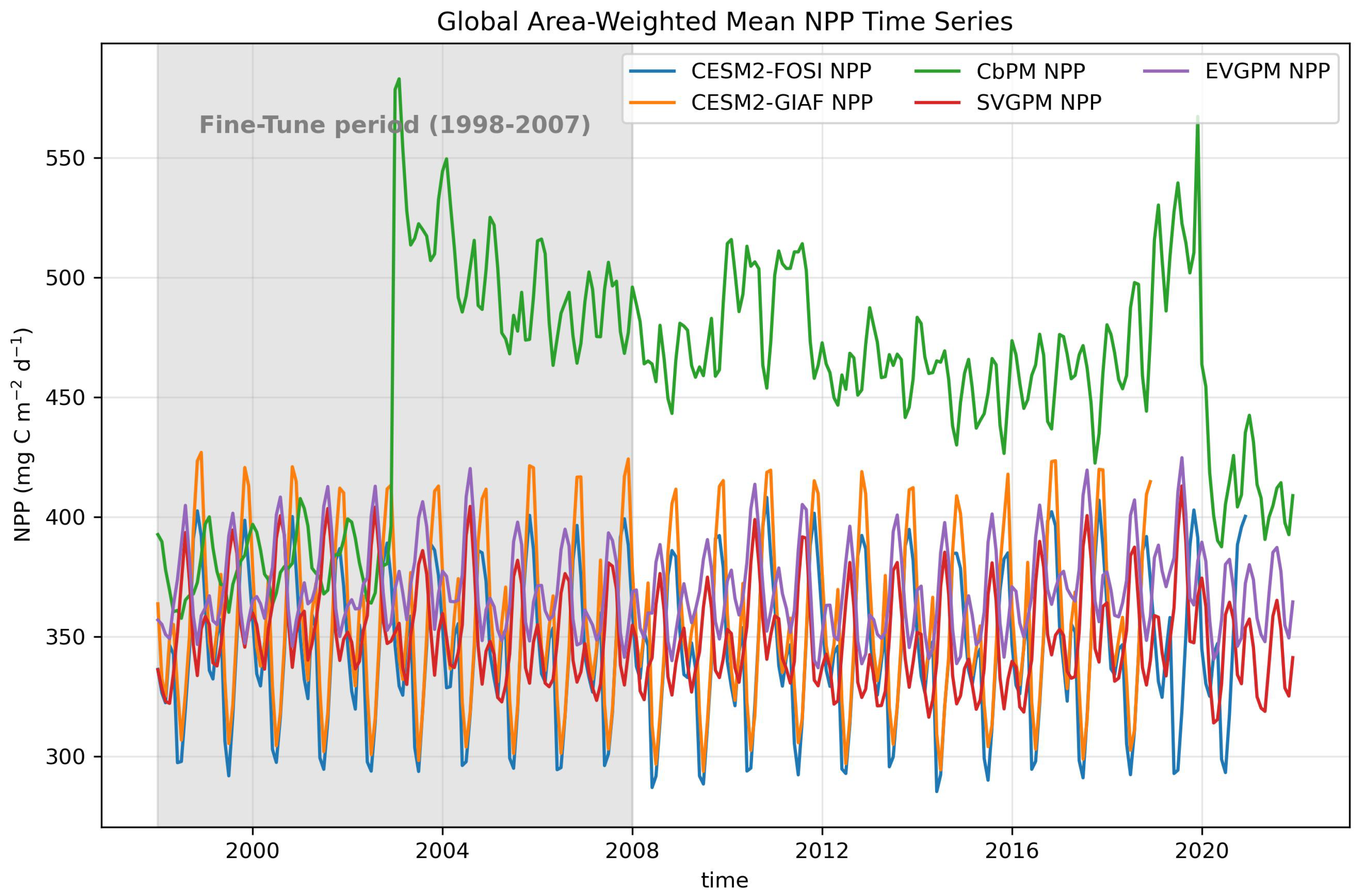
The results indicate that NPPCast exhibits a relatively smaller advantage on the CbPM dataset (Figure 3). As shown in the Figure 15, within the NPP time series, the overall values of CbPM are significantly higher than those of the other datasets (e.g., FOSI, GIAF, EVGPM, and SVGPM) and display a distinct upward shift around 2003. This abrupt shift primarily results from the replacement of input satellite sensors used in the CbPM model. Specifically, the SeaWiFS (Sea-viewing Wide Field-of-view Sensor) data were utilized from 1998 to 2002, while MODIS (Moderate Resolution Imaging Spectroradiometer) data have been employed since 2003. Owing to systematic differences between these two sensors, a pronounced discontinuity emerged in the CbPM-derived NPP estimates around 2003. In contrast, the time series of EVGPM and SVGPM demonstrate more stable temporal variations, with both their magnitudes and seasonal fluctuation patterns remaining highly consistent with the reference datasets used for model pre-training (such as FOSI and GIAF).
Figure 15.
Temporal evolution of NPP from pre-trained datasets (CESM2-FOSI and CESM2-GIAF) and satellite-derived products (CbPM, SVGPM, and EVGPM). The shaded area represents the Fine-Tune period (1998–2007).
In this study, the data used for fine-tuning covered the period from 1998 to 2007 (the shaded area), while the model’s prediction outputs extended beyond this range. Due to the substantial deviation in the time-series characteristics of CbPM from those of the pre-trained model data—particularly the pronounced increase around 2003 and the subsequent sustained high-value state—the model struggled to learn stable temporal relationships during the fine-tuning process. The feature distribution preferences established during pre-training were not well aligned with the statistical properties of the CbPM dataset, leading to a mismatch between the parameter update direction during fine-tuning and the target data distribution. Consequently, this inconsistency weakened the model’s generalization ability in the subsequent prediction period.
In contrast, the time-series characteristics of EVGPM and SVGPM are more consistent with those of the pre-training data. Both in terms of numerical magnitude and seasonal periodicity, these datasets exhibit a high degree of similarity to the pre-training data. This relatively small distributional difference allows the model to more effectively transfer the learned feature representations during the Fine-Tuning stage, thereby achieving greater stability and accuracy in subsequent predictions.
In conclusion, the relatively poor performance of NPPCast on the CbPM dataset is primarily attributed to the substantial distributional inconsistency between CbPM and the pre-trained model data, as well as the abrupt temporal variations observed in the time series. These discrepancies in data distribution and temporal structure directly influence the model’s feature transfer and generalization capabilities, leading to notable differences in NPP prediction results across datasets. It should be noted that our validation suite is representative rather than exhaustive to keep the present study focused on the modeling framework. The NPPCast pipeline itself is agnostic to the target data family and can be extended to other satellite-derived NPP algorithms (e.g., AbPM) after grid and time harmonization, which may help reduce systematic biases among datasets and improve NPP prediction skill at both global and regional scales.
4.2. AttUNet RMSE Spikes and High-RMSE Bands
Attention-UNet (AttUNet) exhibits mid-lead RMSE peaks (e.g., around months ∼14 and ∼19 in Figure 4) and pronounced high-RMSE bands (Figure 11 and Figure 12). We hypothesize three interacting causes: (i) Gate instabilities. Attention gates occasionally saturate or mis-weight features, yielding heavy-tailed residuals and sporadic negative NPP outputs that inflate RMSE when outliers occur. (ii) Seasonal phase drift. At multi-month leads, predicted seasonal cycles can become dephased relative to observations; error then amplifies at specific leads until re-alignment, producing the observed diagonal/banded structures. (iii) Variance amplification. The attention mechanism tends to over-weight high-variance regimes (e.g., equatorial Pacific, western boundary currents, subpolar fronts); when these regions undergo rapid regime shifts, mis-weighted features propagate into larger errors along particular lead–latitude bands.
These mechanisms are not mutually exclusive and likely interact: phase drift sets up lead-specific amplification, while attention mis-weighting magnifies errors where background variability is largest. This interpretation is consistent with the spatial distribution of high-RMSE bands and their coincidence with dynamically energetic regions.
4.3. Potential Application Scenarios of the Prediction Model
We systematically evaluated the performance of NPPCast across temporal and spatial scales from different perspectives. The results show that ACC is generally high in open ocean regions worldwide, with particularly strong performance in high-latitude zones and subpolar gyres, indicating that it can effectively capture relative variations and anomalies on seasonal to interannual timescales. In contrast, ACC in the mid-low latitude regions are relatively low. This may be mainly because the environmental conditions in these areas are relatively stable and the variability of NPP is weak. Consequently, even minor deviations in model predictions can lead to a noticeable reduction in the correlation between the predicted and observed values. RMSE values reveal that the smallest errors occur in the centers of subtropical oligotrophic gyres, suggesting that the model exhibits higher simulation accuracy in these regions. However, the RMSE values are considerably larger in the high-latitude and coastal regions, which may be attributed to observational uncertainties, model limitations, and the pronounced spatiotemporal variability of NPP. Satellite-derived data in these regions usually have higher retrieval errors due to sea ice, cloud, and suspended particles, reducing inversion accuracy. Meanwhile, NPP in these areas exhibits strong spatial and temporal fluctuations, typically corresponding to high-productivity zones. In addition, the Earth system model data used for training often simplify key processes such as upwelling, further increasing the uncertainty of model simulations.
Based on the above results, we suggest that in high-latitude and high-variability regions, research efforts should primarily focus on anomaly and trend detection. These regions are strongly influenced by seasonal changes and interannual climate fluctuations, leading to large variations in NPP []. In these areas, NPPCast exhibits relatively high anomaly correlation coefficients, indicating its strong capability to capture the relative variation trends of phytoplankton. Therefore, the NPPCast model is particularly suitable for studies involving anomaly identification, ecosystem response analysis, and extreme event monitoring on seasonal to interannual timescales. For example, the model outputs can be used to track changes in the intensity and timing of spring phytoplankton blooms, identify years of abnormally high or low productivity, and thereby support marine ecosystem assessments and fisheries resource early warning systems.
In contrast, in mid-low latitude regions, NPPCast exhibits relatively low RMSE, indicating higher accuracy and stability in reproducing the absolute magnitude of NPP. The environmental conditions in these regions are relatively stable, and the interannual variability of NPP is generally small []. Consequently, the model’s predictions are more reliable and suitable for applications that require high accuracy in absolute values, such as marine carbon sink assessments and long-term productivity monitoring. In these contexts, the absolute outputs of the model can be directly used for quantitative analyses, providing a robust data foundation for evaluating marine ecosystem carbon budgets, formulating resource management strategies, and promoting sustainable ocean governance.
This study employs a single variable prediction approach, without incorporating physical or biogeochemical variables into the model. Future research could integrate environmental factors closely related to phytoplankton growth dynamics—such as SST, light availability, and nutrient concentrations—to provide stronger physical constraints on ecosystem processes and thereby enhance the model’s simulation and predictive capabilities. In addition, the current model’s spatial resolution is relatively coarse, limiting its ability to accurately resolve mesoscale dynamical processes that significantly influence net primary productivity. Future work could utilize higher-resolution data to more precisely represent small-scale ocean dynamics, thereby reducing model errors in regions with strong environmental variability and improving the model’s ability to simulate local ecological processes.
5. Conclusions
In summary, the proposed NPPCast model substantially advances the predictive capability of marine NPP forecasting on seasonal to multi-year timescales. Compared with representative UNet-family architectures, NPPCast consistently achieves lower global RMSE, higher ACC, and superior spatial and structural fidelity across multiple satellite-derived NPP products. It maintains robust predictive skill across both VGPM- and CbPM-based targets, though its performance varies moderately among products due to differences in their underlying algorithms. These variations reflect the inherent diversity of empirical formulations in satellite-based NPP estimation rather than limitations of the proposed architecture. Since our primary focus lies in the modeling advance itself rather than in product-specific optimization, the satellite products used for fine-tuning and validation serve as representative rather than exhaustive datasets here. A key strength of NPPCast lies in its causal dilated-convolution framework and transfer learning design, which together yield more accurate, stable, and transferable predictions. The model demonstrates exceptional robustness, maintaining nearly identical performance when initialized with different climate simulation data, highlighting exceptional stability and scene-robustness. Importantly, NPPCast’s grouped convolutional design allows it to capture physically meaningful patterns across neighboring regions, addressing the opaque “pointwise attribution” issue of standard CNNs. Collectively, these advances make NPPCast a powerful, efficient, and more interpretable model for long-term global ocean productivity forecasting. Future work will explore its applications to other biogeochemical fields and further improve the mechanistic understanding of its predictions.
Author Contributions
Conceptualization, Z.L., B.W., Z.Y., R.C., and S.W.; methodology, B.W. and Z.L.; software, B.W.; validation, B.W. and Z.L.; formal analysis, B.W. and Z.L.; investigation, B.W.; resources, S.W.; data curation, Z.L., B.W., Z.Y., and R.C.; writing—original draft preparation, B.W. and Z.L.; writing—review and editing, Z.L., B.W., Z.Y., R.C., and S.W.; visualization, B.W. and Z.L.; supervision, S.W.; project administration, S.W.; funding acquisition, S.W. All authors have read and agreed to the published version of the manuscript.
Funding
This research was funded by the National Natural Science Foundation of China (NSFC) under grant numbers 42430404, 42376233, and the Research Grants Council of the Hong Kong Special Administrative Region, China (Project Reference No. AoE/P-601/23-N).
Data Availability Statement
Output from the Community Earth System Model version 2 Seasonal-to-Multiyear Large Ensemble (CESM2-SMYLE) can be downloaded at https://rda.ucar.edu/datasets/d651065/dataaccess/ (accessed on 1 November 2025). All code used to produce the results in this paper is openly available at the project repository: https://github.com/wubizhi/NPPCast (accessed on 1 November 2025). The repository contains experiment scripts, model definitions, preprocessing utilities, and plotting notebooks to reproduce all figures and tables. The analysis code and datasets supporting the findings of this study are archived on Zenodo and can be accessed at [].
Acknowledgments
The authors gratefully acknowledge support from the Technician Development Fund of the State Key Laboratory of Marine Environmental Science, Xiamen University.
Conflicts of Interest
The authors declare no conflicts of interest.
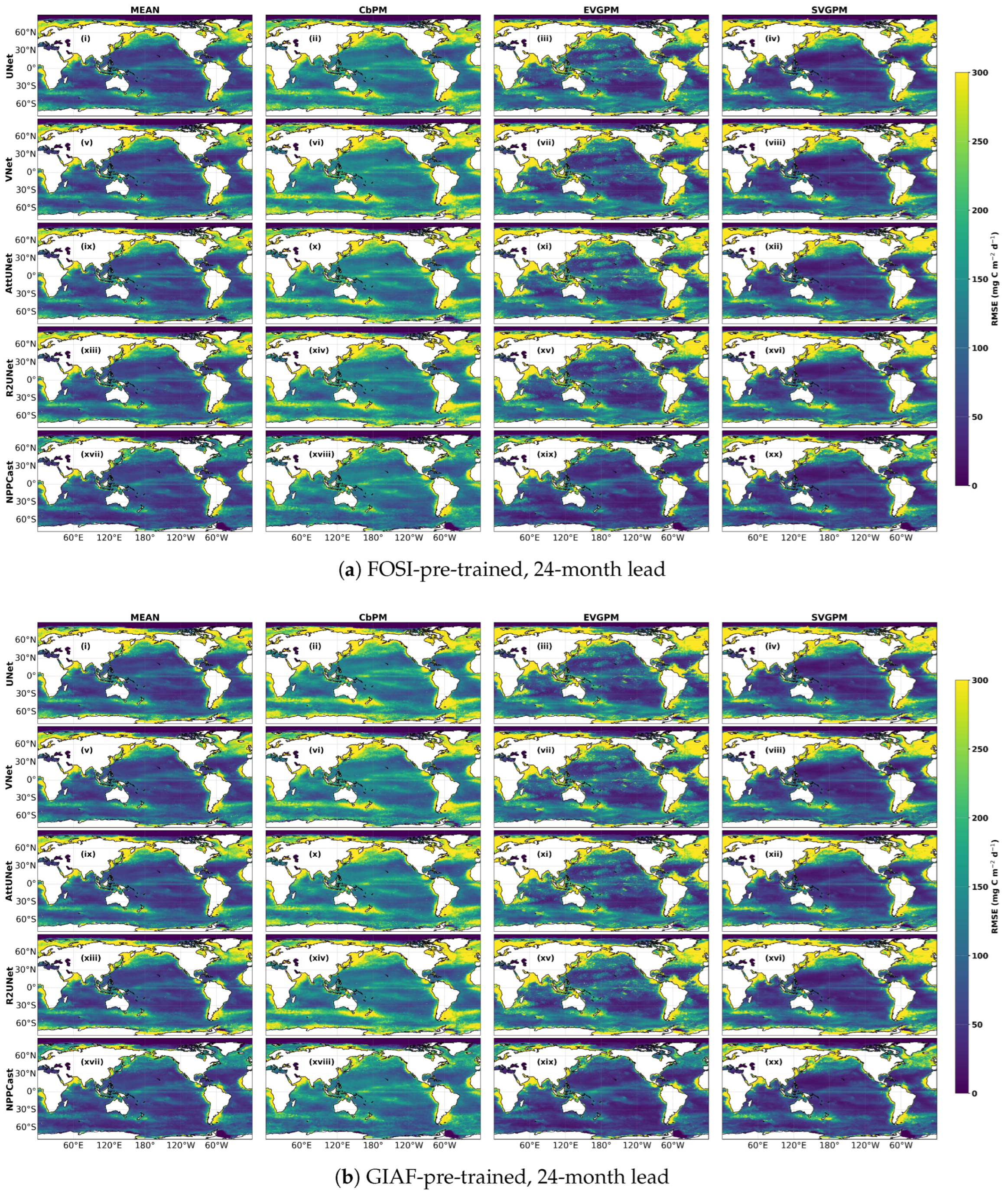
Appendix A. Spatial Pattern Fidelity at 24-Month Lead (FOSI and GIAF Pretraining)
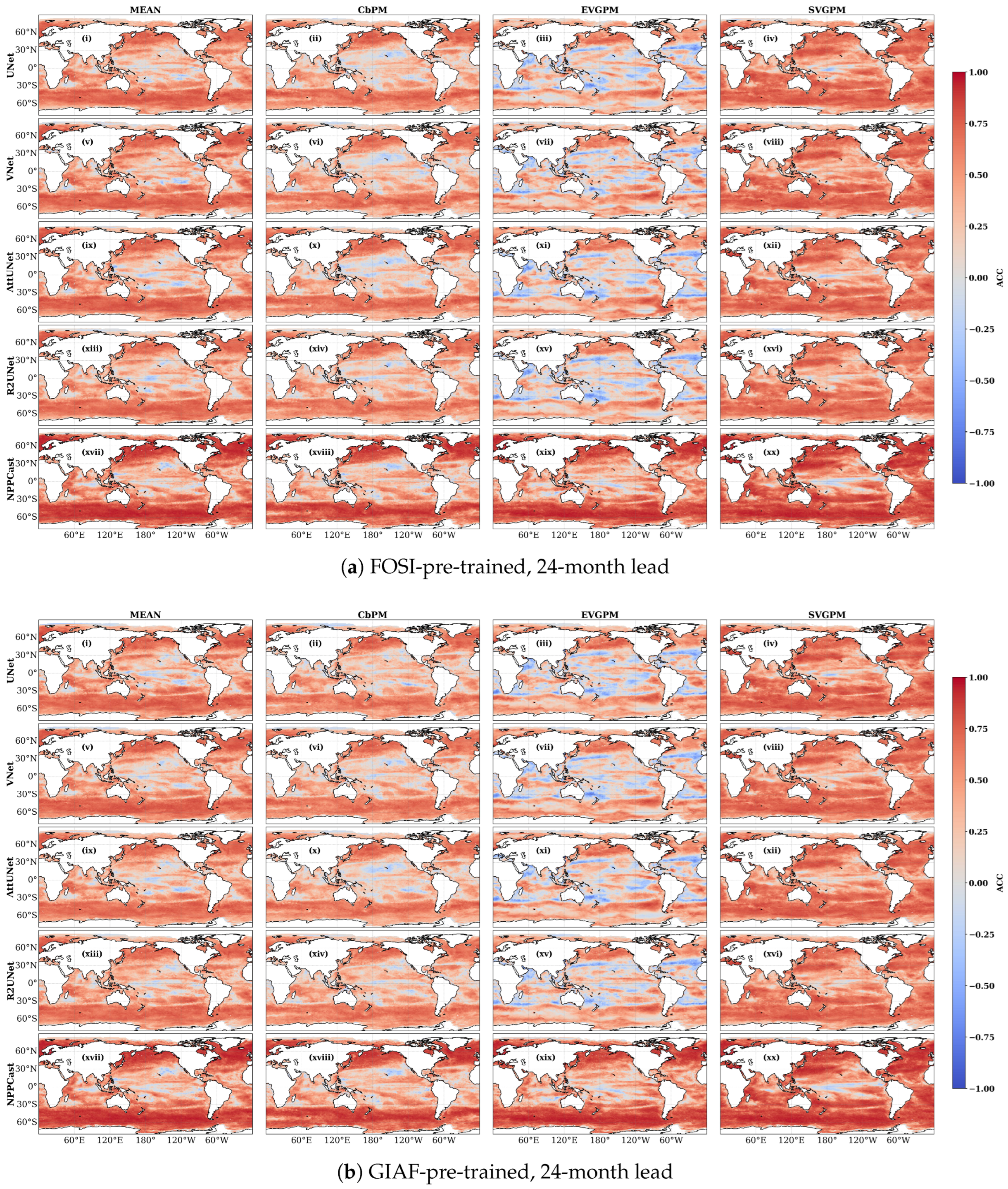
Moving to lead-24 (Figure A1), overall ACC drops for all models, but the pattern differences sharpen. In the FOSI-pretrained maps, NPPCast still shows moderate ACC (light-to-medium warm tones) over the subtropical-extratropical Pacific and Atlantic basins in both hemispheres, while the UNet-family ACC has largely collapsed to near zero (near-gray) in those same regions. Similarly, in the GIAF-pretrained maps, NPPCast maintains discernible ACC bands along the eastern Indian–western Pacific sector and the mid-latitude Atlantic, whereas UNet variants show almost no coherent signal. In both datasets, the relative advantage of NPPCast becomes more pronounced by lead-24: NPPCast’s ACC remains on the order of 0.2–0.4 in favorable regions (e.g., western North America, far North Atlantic, southern Pacific), while UNets have mostly lost spatial correlation. Latitudinally, the subtropics (20–40° in each hemisphere) consistently exhibit the slowest skill decay; NPPCast in particular preserves pattern fidelity here (orange/red shading) longer than any UNet model.
Figure A1.
Same layout as Figure 5 but for a 24-month lead (UNet (i–iv), VNet (v–viii), AttUNet (ix–xii), R2UNet (xiii–xvi), NPPCast (xvii–xx)). While the four UNet-family baselines now lose considerable skill (large blue patches in subtropical gyres and the Southern Ocean), NPPCast maintains coherent positive ACC over most basins, highlighting its markedly slower spatial- skill decay.
At 24-month lead time, all models exhibit an overall increase in RMSE, indicating that forecast errors grow as the prediction horizon extends. Despite this increase, the spatial distribution patterns of RMSE remain consistent across models: RMSE are lowest in the subtropical gyre open oceans, while high-latitude and continental margin regions show substantially higher RMSE, reflecting the greater variability and prediction difficulty of NPP in these dynamic areas. Compared with the CbPM product, the other reference products display relatively lower errors within the subtropical gyre regions. NPPCast demonstrates the best performance across most global open ocean regions, yielding the lowest RMSE values. However, in high-latitude and coastal upwelling regions, NPPCast still shows noticeably larger RMSE, suggesting that these high-variability areas remain the primary challenge for long-lead NPP prediction.
Figure A2.
Same layout as Figure 7 but for a 24-month lead (UNet (i–iv), VNet (v–viii), AttUNet (ix–xii), R2UNet (xiii–xvi), NPPCast (xvii–xx)).
Appendix B. Comparison Between CESM2-SMYLE and NPPCast in Predicting NPP
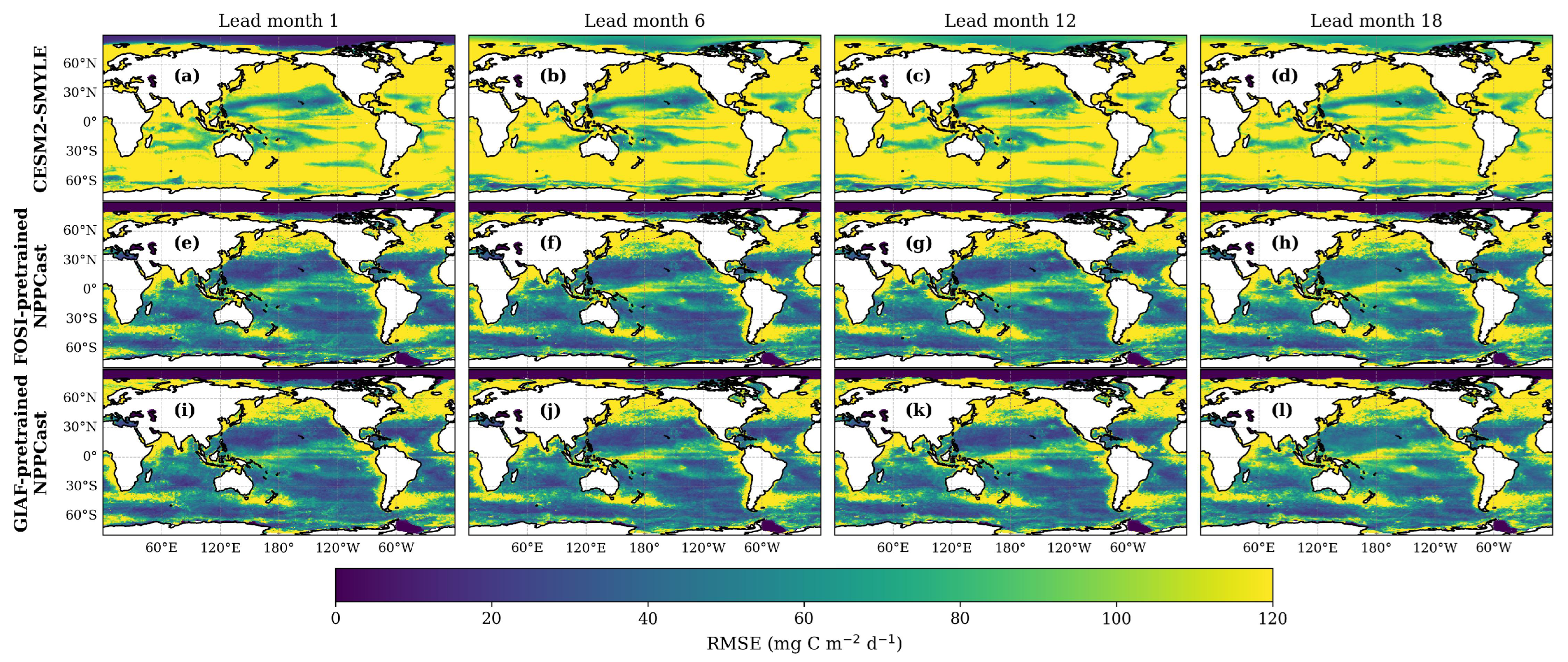
Figure A3 shows the spatial distribution of RMSE in NPP forecasts from CESM2-SMYLE and two versions of the NPPCast model at different lead times (1, 6, 12, and 18 months). Across all lead times, the NPPCast models show broader regions of lower RMSE relative to CESM2-SMYLE, indicating differences in spatial error characteristics between the machine learning and Earth system model. These differences are particularly pronounced in the tropical Pacific, Southern Ocean, and major eastern boundary upwelling systems—areas characterized by high biogeochemical variability. Notably, even at extended lead times of 12 and 18 months, the NPPCast models maintain relatively low RMSE.
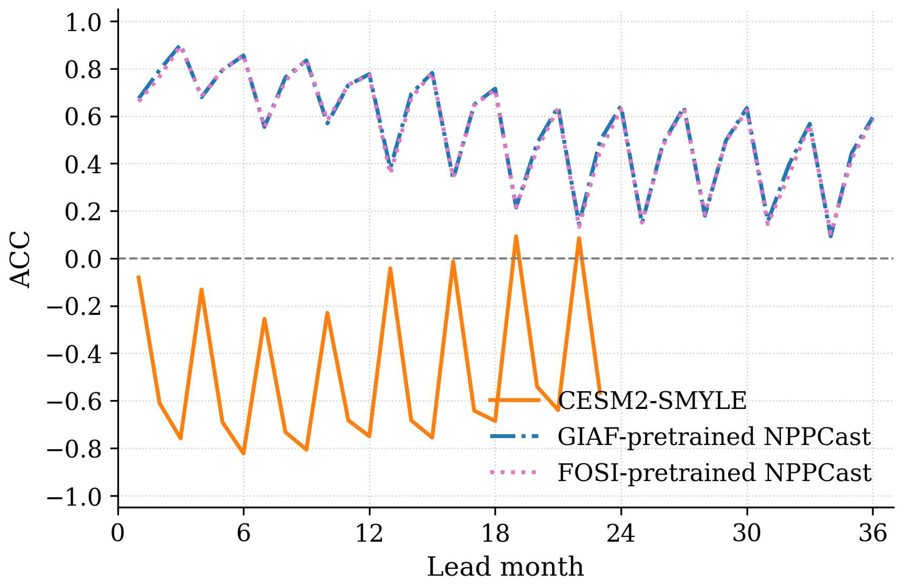
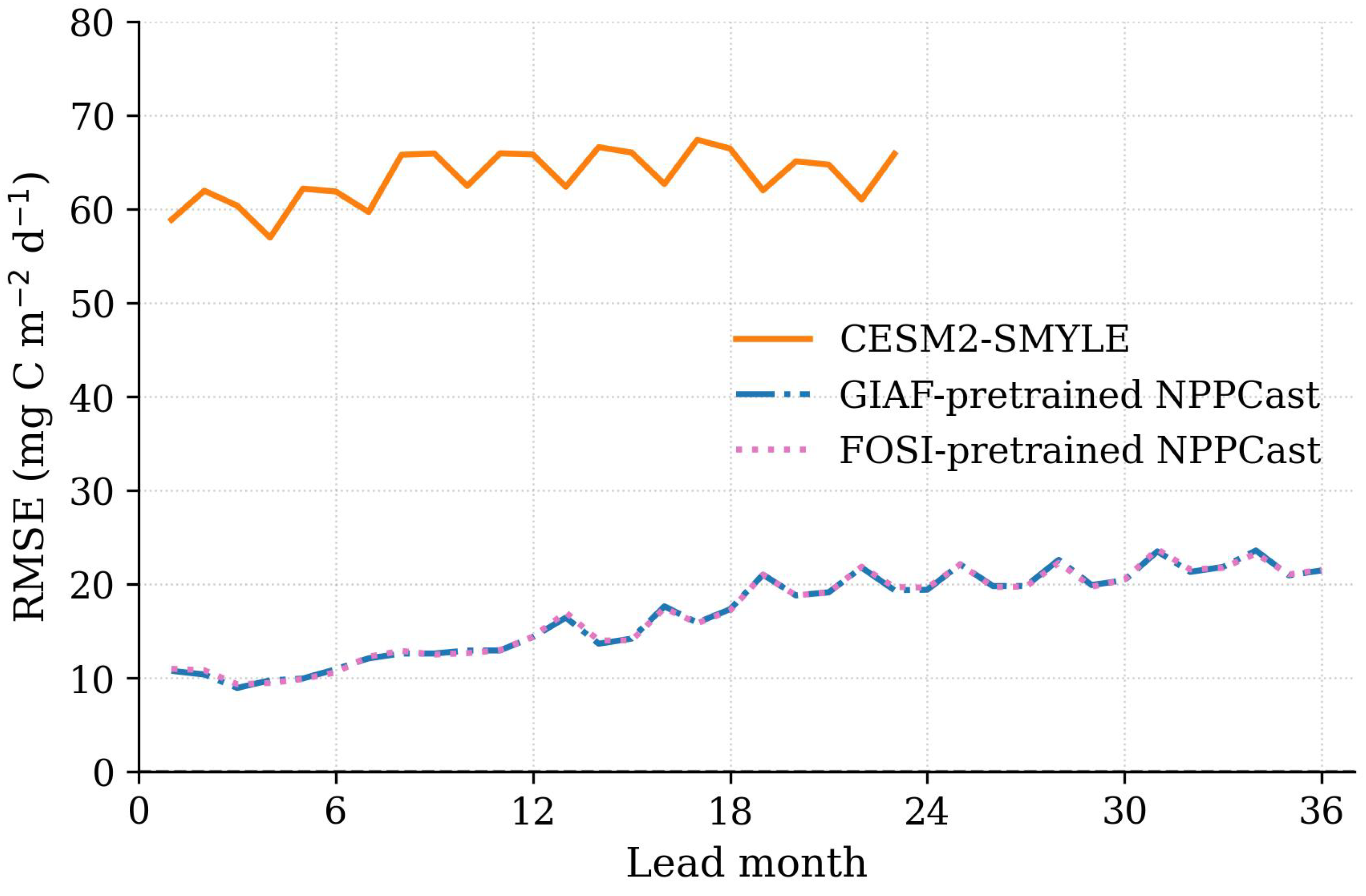
Over the lead time 1–36 months, the NPPCast models exhibit relatively stable prediction skill, with most lead times exhibiting ACC values above 0.4 and RMSE values remaining below 18 mg C (Figure A4 and Figure A5). In contrast, CESM2-SMYLE demonstrates larger variations in prediction skill across lead times, with generally low ACC values that frequently drop below zero, and markedly higher RMSE values typically exceeding 60 mg C .
It should be noted that this comparison is illustrative only, intended to highlight qualitative spatial–temporal differences rather than to establish a strict quantitative benchmark.
Figure A3.
Spatial distribution of RMSE for NPP forecasts CESM2-SMYLE (a–d), FOSI-pretrained NPPCast (e–h), and GIAF-pretrained NPPCast (i–l) models at lead months 1, 6, 12, and 18.
Figure A4.
Lead-time evolution of ACC for global area-weighted average NPP forecasts from CESM2-SMYLE and NPPCast models.
Figure A5.
Lead-time evolution of RMSE for global area-weighted average NPP forecasts from CESM2-SMYLE and NPPCast models.
Appendix C. Attention-Gating Instability in Global Ocean NPP Forecasting
Appendix C.1. Phenomenology
Across products and pre-training scenes, AttUNet exhibits two recurring artefacts that are largely absent from the other UNet baselines and from NPPCast: (i) discrete troughs in lead–wise ACC at specific months ahead and (ii) latitude-spanning bands of elevated RMSE that recur at the same leads in the Hovmöller diagrams. These events cluster near harmonics or offsets of the annual cycle (e.g., ∼14, 19 months in FOSI; ∼4, 23, 28 months in GIAF), and coincide with abrupt loss of spatial correlation.
Appendix C.2. Mechanistic Hypothesis: Attention-Gate Phase Locking
AttUNet augments UNet with attention gates (AGs) on encoder–decoder skip connections. Each gate computes a sigmoid weight field by matching query features from the decoder with key/value features from the encoder; the weighted skip is then added to the decoder state. During autoregressive roll-out for multi-month forecasting, these gates are recomputed at every step from the model’s own prior predictions. Small phase errors in the seasonal cycle at one step perturb the decoder queries; because the sigmoid gate is highly non-linear, this can saturate the gate toward suppressing (or over-amplifying) entire skip paths. Once the skip information is muted across broad regions, the decoder relies on coarser, slowly varying features, causing an effective phase shift of ∼1–2 months. The spatial correlation then collapses abruptly (ACC dips), and the error becomes nearly zonally coherent (bright RMSE bands), reflecting the latitude-coherent seasonal mode rather than a local amplitude failure.
This hypothesis is consistent with three observations:
- Lead clustering: the failures concentrate near seasonal harmonics or offsets, a signature of phase misalignment rather than random noise.
- Zonal uniformity: at failure leads the RMSE band spans most latitudes, matching the global seasonal mode seen in the Hovmöller plots.
- Between–event behavior: AttUNet’s RMSE between dips is comparable to other UNets; the degradation is intermittent and gate-triggered, not a constant amplitude bias.
Appendix C.3. Evidence from AttUNet Outputs at Failure Leads
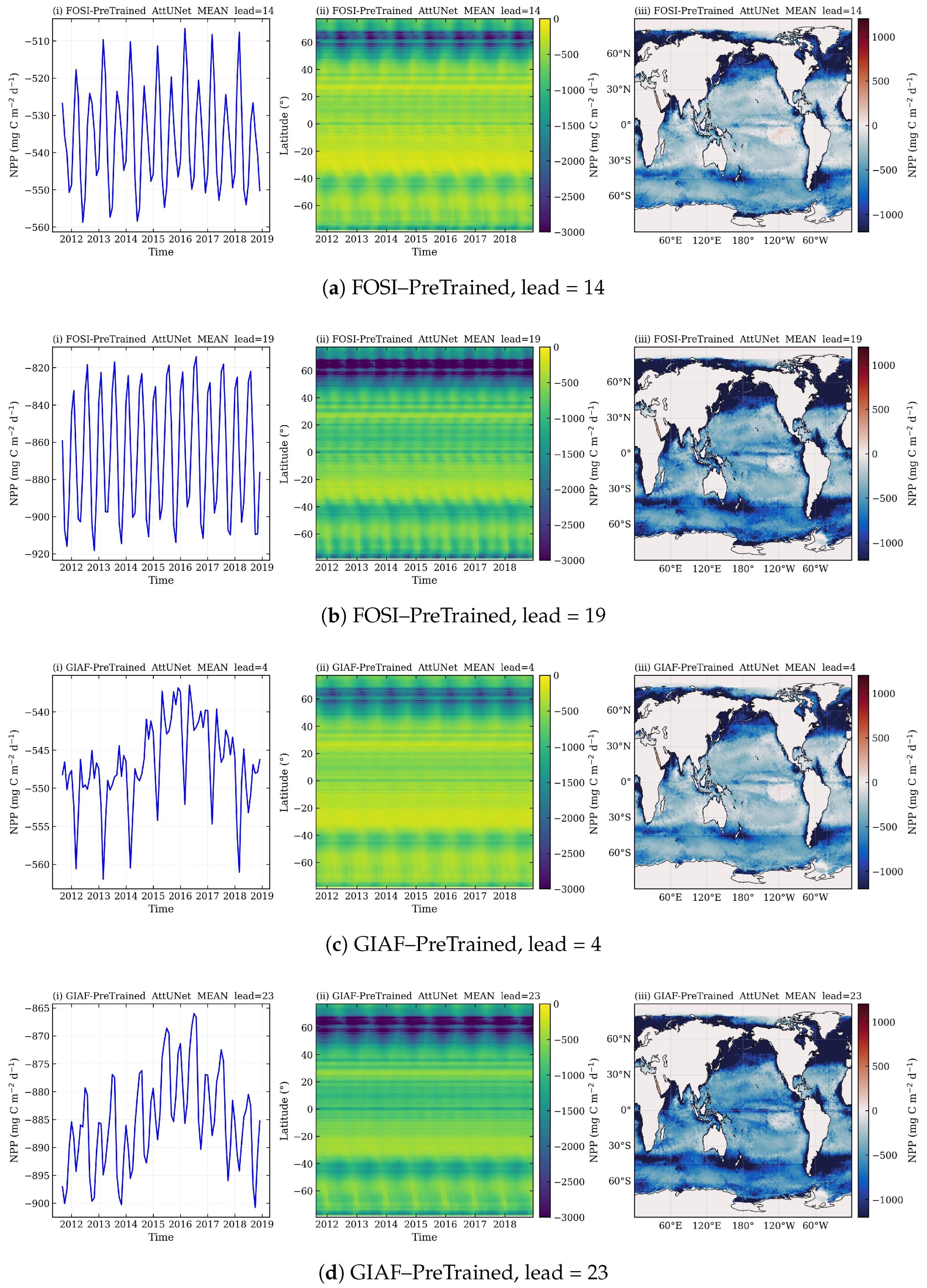
Figure A6 illustrates five representative failure leads. For each case (panels i–iii within each subfigure) we show: (i) the globally averaged predicted NPP time series; (ii) the latitude–time Hovmöller of predicted NPP; and (iii) the corresponding global NPP map. The problematic leads exhibit abrupt phase shifts in the global time series, enhanced, latitude-wide seasonal bands in the Hovmöller view, and broad, zonal striping in the map view—consistent with gate saturation and phase locking.

Figure A6.
AttUNet failure signatures at selected leads. Each composite image contains (left) global-mean predicted NPP time series, (middle) latitude–time Hovmöller, and (right) global map. The events display abrupt phase shifts, latitude-coherent bands, and zonal striping—hallmarks of attention-gate saturation and phase locking during autoregressive roll-out. Identified leads (FOSI: 14 (a), 19 (b); GIAF: 4 (c), 23 (d), 28 (e)) coincide with the ACC troughs and RMSE bands reported in the main figures.
Appendix C.4. Why AttUNet Is Uniquely Vulnerable
Unlike plain UNet/VNet/R2UNet, AttUNet modulates skip information multiplicatively. When the gate’s alignment drifts due to a small phase error, the sigmoid can saturate near 0 or 1, effectively switching off (or over-emphasizing) high-frequency, seasonally keyed features provided by the skip. In an autoregressive setting this becomes a positive feedback: a slightly mis-timed seasonal signal yields poorer alignment at the next step, further suppressing useful skips and pushing the phase farther off, producing discrete collapses in ACC and latitude-wide RMSE bands. NPPCast avoids this pathology because it (i) does not rely on attention-gated skips, (ii) predicts regionally grouped multivariate time series with causal convolutions that preserve phase information, and (iii) trains with multi-step objectives that reduce exposure bias.
Appendix D. Interpreting Negative R2 and a Positive-Only Sanity Check
Appendix D.1. Definition and Implication
We compute the coefficient of determination as
following standard usage in statistics and machine learning (see, e.g., []) (under this definition, can be negative, with no lower bound. Values occur when , i.e., the model’s mean–squared error is more than twice that of the “predict-the-mean” baseline). Thus, whenever the residual variance exceeds the variance of the truth, becomes negative.
Appendix D.2. Visual Diagnosis from Scatter Plots
Figure 9, Figure 10, Figure A7 and Figure A8 compare predicted versus observed NPP for all models and products under two visualization settings: (i) retaining all predictions—including physically implausible negative values (Figure 9 and Figure 10)—and (ii) censoring predictions (<0) as a positive-only sanity check (Figure A7 and Figure A8). Two consistent findings emerge:
- UNet-family baselines (UNet, VNet, AttUNet, R2UNet) produce a non-trivial number of negative NPP predictions. These negatives inflate and directly explain the highly negative values (occasionally ) in the “keep-all” panels.
- NPPCast rarely yields negative outputs; removing negatives changes its only marginally. This stability aligns with the higher, positive reported across products.
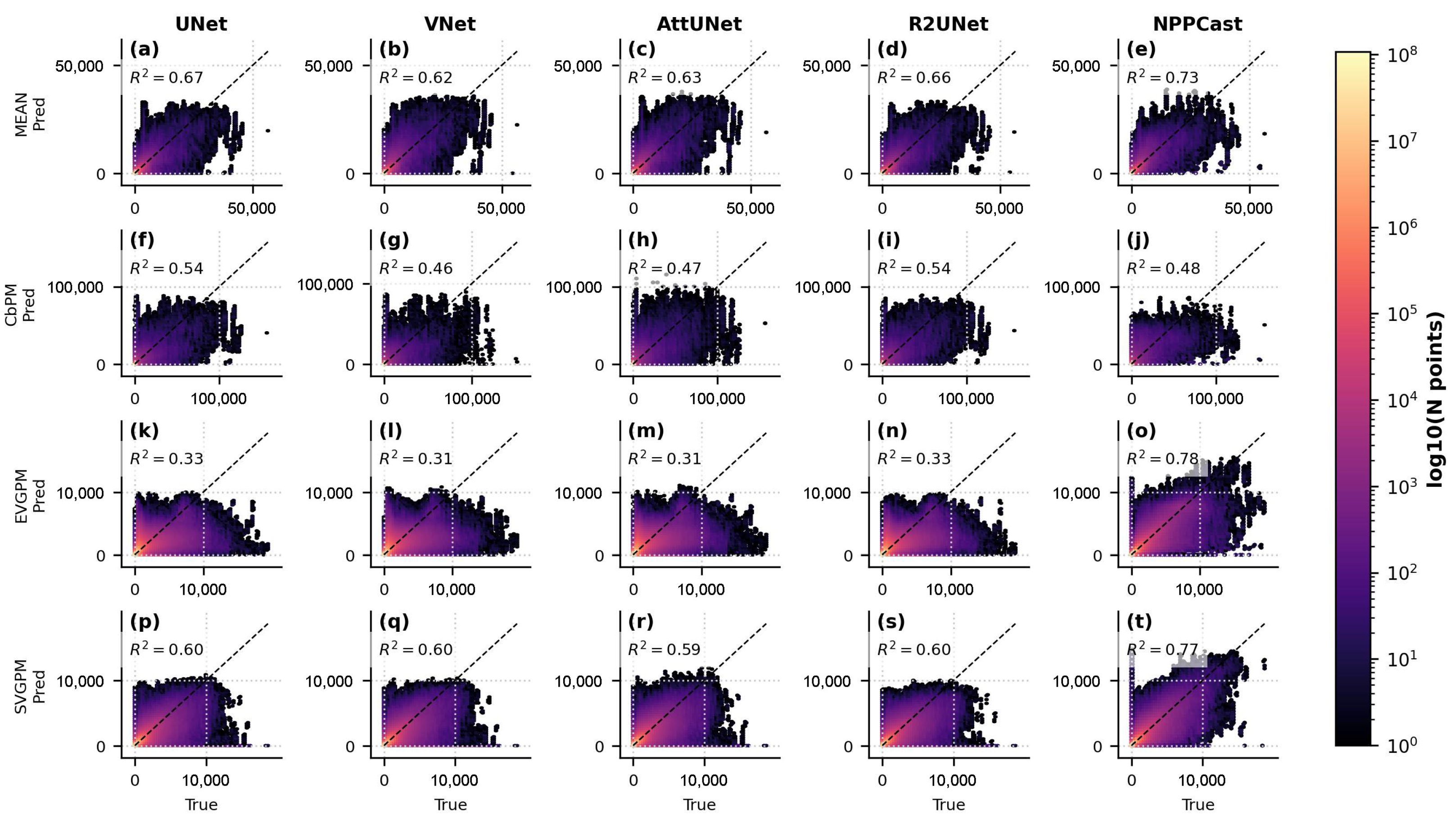
For transparency, we retain the original predictions (including negatives) in the main comparison and report accordingly, while providing the positive-only companion views here to isolate the impact of unphysical negatives. All axes now include complete labels, scales, and units.
Figure A7.
FOSI pretraining (negatives removed). Same as Figure 9 but censoring predictions (rows: MEAN (a–e), CbPM (f–j), EVGPM (k–o), SVGPM (p–t)). for UNet-family models increases substantially; NPPCast changes only slightly, confirming that extreme negative values mainly originate from negative predictions in the baselines.
Figure A8.
GIAF pretraining (negatives removed). Same as Figure 10 but censoring predictions (rows: MEAN (a–e), CbPM (f–j), EVGPM (k–o), SVGPM (p–t)). UNet-family improves markedly; NPPCast remains nearly unchanged.
Appendix E. Spatial Partitioning in NPPCast—Definition, Rationale, and G-Invariance
This note formalizes NPPCast’s spatial partitioning and provides a theory-first justification that the number of regional groups G is an engineering (compute/batching) parameter rather than a scientific hyperparameter: under standard assumptions, the forecasting accuracy is invariant to G.
Appendix E.1. Setup and Notation
Let denote a monthly data cube on a latitude–longitude grid, and let be an ocean–land mask. After masking, the set of valid ocean pixels is
For each pixel , let be the scalar NPP at time t. Given a forecast window length L and horizon , we form (per pixel) input–target pairs from sliding windows.
Appendix E.2. Partitioning Operator and Regional Construction
A partition of into G disjoint, contiguous tiles satisfies
Contiguity preserves geographic coherence and avoids non-physical mixing of distant provinces; approximately equal tile sizes secure sufficient samples per region to stabilize seasonal phase and low-frequency variability.
For region g, we assemble a multivariate time series of all its pixels:
A TimesNet-based regional forecaster
produces for the same set of pixels . Predictions are scattered back to the global grid by identity remap, followed by a light per-pixel affine fusion to correct small biases; because the sets are disjoint, each pixel receives exactly one regional forecast before fusion.
Appendix E.3. Objective and Loss Decomposition
Let be the collection of all regional training windows. The learning objective is an area-weighted, per-pixel additive loss:
with nonnegative weights (e.g., proportional to cell area or ), and a convex pointwise loss ℓ (e.g., MAE/MSE). Equivalently, , i.e., the loss decomposes per pixel (and lead).
Appendix E.4. Two Assumptions
We state two conditions; either one alone suffices for G-invariance.
- Channel-separable temporal core with permutation-equivariant mixing.
The regional TimesNet uses depthwise temporal operators (per-channel temporal feature extractors) and cross-channel mixing that is permutation-equivariant (e.g., a shared linear mixing layer), applied identically regardless of channel order. Consequences:
- Permutation invariance across channels: Re-indexing or re-grouping channels leaves the function class unchanged; the network receives the same set of per-pixel sequences regardless of how they are grouped during batching.
- Direct-sum structure: The global mapping can be written as a direct sum of identical local operators applied at all pixels. Partitioning the channels into different contiguous segments (changing G) does not alter this direct-sum operator; it only changes the data-loading bookkeeping.
- B.
- Local neighborhood rule independent of G.
If any cross-channel operation is local (e.g., mixing within a geodesic radius R around each pixel), and each tile is chosen contiguous with margin so that every pixel’s neighborhood is fully contained within its tile, then the learned operator at each pixel depends only on its local neighborhood, not on the tile index.
In NPPCast as implemented, both A and B hold: temporal cores are channel-separable with permutation-equivariant mixing, and tiles are contiguous and sufficiently wide relative to any local mixing; the fusion is per-pixel (), so there is no cross-region averaging that could smear boundaries. Under either condition A or B, the loss decomposes per pixel (and its local neighborhood), and the same local operator is applied everywhere; therefore, the partitioning affects memory layout only, not predictive accuracy.
Appendix E.5. Practical Implications and Choice of G in This Study
Compute/batching role of G: The value of G is chosen to saturate GPU memory at the desired window length L and embedding depth, thereby improving optimizer stability and throughput. In this manuscript we use micro-regions on the CESM nominal ocean grid (after land masking), which saturates an NVIDIA A40 (48 GB) at with our TimesNet-based setting.
Receptive fields: The temporal receptive field per regional forecaster is months (3 years). The effective spatial footprint equals the extent of its tile ; this footprint reflects sharding for compute and does not constitute a scientific hyperparameter.
Fusion and boundaries: Final reconstruction uses an identity remap and a per-pixel affine correction. Because tiles are disjoint and fusion is per-pixel, there is no cross-region averaging and boundary effects are negligible.
Summary: Under NPPCast’s design (channel-separable temporal cores with permutation-equivariant mixing; contiguous tiles with sufficient margin; per-pixel additive loss and per-pixel fusion), forecasting accuracy does not depend on G. The partition is a compute device; different G values alter memory layout and throughput but not the modeling assumptions nor the attainable accuracy.
References
- Field, C.B.; Behrenfeld, M.J.; Randerson, J.T.; Falkowski, P. Primary production of the biosphere: Integrating terrestrial and oceanic components. Science 1998, 281, 237–240. [Google Scholar] [CrossRef]
- Kwon, E.Y.; Primeau, F.; Sarmiento, J.L. The impact of remineralization depth on the air–sea carbon balance. Nat. Geosci. 2009, 2, 630–635. [Google Scholar] [CrossRef]
- Stock, C.A.; John, J.G.; Rykaczewski, R.R.; Asch, R.G.; Cheung, W.W.; Dunne, J.P.; Friedland, K.D.; Lam, V.W.; Sarmiento, J.L.; Watson, R.A. Reconciling fisheries catch and ocean productivity. Proc. Natl. Acad. Sci. USA 2017, 114, E1441–E1449. [Google Scholar] [CrossRef]
- Behrenfeld, M.J.; Falkowski, P.G. Photosynthetic rates derived from satellite-based chlorophyll concentration. Limnol. Oceanogr. 1997, 42, 1–20. [Google Scholar] [CrossRef]
- Behrenfeld, M.J.; Boss, E.; Siegel, D.A.; Shea, D.M. Carbon-based ocean productivity and phytoplankton physiology from space. Glob. Biogeochem. Cycles 2005, 19, GB1006. [Google Scholar] [CrossRef]
- Westberry, T.; Behrenfeld, M.; Siegel, D.; Boss, E. Carbon-based primary productivity modeling with vertically resolved photoacclimation. Glob. Biogeochem. Cycles 2008, 22, GB2024. [Google Scholar] [CrossRef]
- Lee, Z.; Carder, K.; Marra, J.; Steward, R.; Perry, M. Estimating primary production at depth from remote sensing. Appl. Opt. 1996, 35, 463–474. [Google Scholar] [CrossRef]
- Behrenfeld, M.J.; O’Malley, R.T.; Siegel, D.A.; McClain, C.R.; Sarmiento, J.L.; Feldman, G.C.; Milligan, A.J.; Falkowski, P.G.; Letelier, R.M.; Boss, E.S. Climate-driven trends in contemporary ocean productivity. Nature 2006, 444, 752–755. [Google Scholar] [CrossRef]
- Laufkötter, C.; Vogt, M.; Gruber, N.; Aita-Noguchi, M.; Aumont, O.; Bopp, L.; Buitenhuis, E.; Doney, S.C.; Dunne, J.; Hashioka, T.; et al. Drivers and uncertainties of future global marine primary production in marine ecosystem models. Biogeosciences 2015, 12, 6955–6984. [Google Scholar] [CrossRef]
- Moore, C.; Mills, M.; Arrigo, K.; Berman-Frank, I.; Bopp, L.; Boyd, P.; Galbraith, E.; Geider, R.; Guieu, C.; Jaccard, S.; et al. Processes and patterns of oceanic nutrient limitation. Nat. Geosci. 2013, 6, 701–710. [Google Scholar] [CrossRef]
- Séférian, R.; Bopp, L.; Gehlen, M.; Swingedouw, D.; Mignot, J.; Guilyardi, E.; Servonnat, J. Multiyear predictability of tropical marine productivity. Proc. Natl. Acad. Sci. USA 2014, 111, 11646–11651. [Google Scholar] [CrossRef]
- Krumhardt, K.M.; Lovenduski, N.S.; Long, M.C.; Luo, J.; Lindsay, K.; Yeager, S.; Harrison, C. Potential predictability of net primary production in the ocean. Glob. Biogeochem. Cycles 2020, 34, e2020GB006531. [Google Scholar] [CrossRef]
- Frölicher, T.L.; Ramseyer, L.; Raible, C.C.; Rodgers, K.B.; Dunne, J. Potential predictability of marine ecosystem drivers. Biogeosciences 2020, 17, 2061–2083. [Google Scholar] [CrossRef]
- Park, J.Y.; Stock, C.A.; Dunne, J.P.; Yang, X.; Rosati, A. Seasonal to multiannual marine ecosystem prediction with a global Earth system model. Science 2019, 365, 284–288. [Google Scholar] [CrossRef]
- Tagliabue, A.; Kwiatkowski, L.; Bopp, L.; Butenschön, M.; Cheung, W.; Lengaigne, M.; Vialard, J. Persistent uncertainties in ocean net primary production climate change projections at regional scales raise challenges for assessing impacts on ecosystem services. Front. Clim. 2021, 3, 738224. [Google Scholar] [CrossRef]
- Wu, X.; Yeager, S.G.; Deser, C.; Rosenbloom, N.; Meehl, G.A. Volcanic forcing degrades multiyear-to-decadal prediction skill in the tropical Pacific. Sci. Adv. 2023, 9, eadd9364. [Google Scholar] [CrossRef]
- Ford, D.; Edwards, K.; Lea, D.; Barciela, R.; Martin, M.; Demaria, J. Assimilating GlobColour ocean colour data into a pre-operational physical-biogeochemical model. Ocean. Sci. 2012, 8, 751–771. [Google Scholar] [CrossRef]
- Yeager, S.; Danabasoglu, G.; Rosenbloom, N.; Strand, W.; Bates, S.; Meehl, G.; Karspeck, A.; Lindsay, K.; Long, M.; Teng, H.; et al. Predicting near-term changes in the earth system: A large ensemble of initialized decadal prediction simulations using the community earth system model. Bull. Am. Meteorol. Soc. 2018, 99, 1867–1886. [Google Scholar] [CrossRef]
- Webster, P.J.; Yang, S. Monsoon and ENSO: Selectively interactive systems. Q. J. R. Meteorol. Soc. 1992, 118, 877–926. [Google Scholar] [CrossRef]
- Levine, A.F.; McPhaden, M.J. The annual cycle in ENSO growth rate as a cause of the spring predictability barrier. Geophys. Res. Lett. 2015, 42, 5034–5041. [Google Scholar] [CrossRef]
- Qi, Q.; Duan, W.; Xu, H. The most sensitive initial error modes modulating intensities of CP-and EP-El Niño events. Dyn. Atmos. Ocean. 2021, 96, 101257. [Google Scholar] [CrossRef]
- Boschetti, F.; Feng, M.; Hartog, J.R.; Hobday, A.J.; Zhang, X. Sea surface temperature predictability assessment with an ensemble machine learning method using climate model simulations. Deep. Sea Res. Part II Top. Stud. Oceanogr. 2023, 210, 105308. [Google Scholar] [CrossRef]
- Reichstein, M.; Camps-Valls, G.; Stevens, B.; Jung, M.; Denzler, J.; Carvalhais, N.; Prabhat, F. Deep learning and process understanding for data-driven Earth system science. Nature 2019, 566, 195–204. [Google Scholar] [CrossRef]
- Shen, Z.; Sun, Q.; Lu, X.; Ling, F.; Li, Y.; Wu, J.; Luo, J.J.; Yuan, C. Current Progress in Subseasonal-to-Decadal Prediction based on Machine Learning. Appl. Comput. Geosci. 2024, 24, 100201. [Google Scholar] [CrossRef]
- Ren, J.; Wang, C.; Sun, L.; Huang, B.; Zhang, D.; Mu, J.; Wu, J. Prediction of sea surface temperature using U-Net based model. Remote Sens. 2024, 16, 1205. [Google Scholar] [CrossRef]
- Ji, X.; Song, X.; Guo, A.; Liu, K.; Cao, H.; Feng, T. Oceanic Precipitation Nowcasting Using a UNet-Based Residual and Attention Network and Real-Time Himawari-8 Images. Remote Sens. 2024, 16, 2871. [Google Scholar] [CrossRef]
- Mohammed, A. ResAttUNet: Detecting marine debris using an attention activated residual UNet. arXiv 2022, arXiv:2210.08506. [Google Scholar] [CrossRef]
- Jamali, A.; Roy, S.K.; Beni, L.H.; Pradhan, B.; Li, J.; Ghamisi, P. Residual wave vision U-Net for flood mapping using dual polarization Sentinel-1 SAR imagery. Int. J. Appl. Earth Obs. Geoinf. 2024, 127, 103662. [Google Scholar] [CrossRef]
- Putra, D.P.; Hsu, P.C. Leveraging Transfer Learning and U-Nets Method for Improved Gap Filling in Himawari Sea Surface Temperature Data Adjacent to Taiwan. ISPRS Int. J.-Geo-Inf. 2024, 13, 162. [Google Scholar] [CrossRef]
- Wang, Y.; Zhang, Y.; Wang, G. Impact of physical and attention mechanisms on U-Net for SST forecasting. Intell. Mar. Technol. Syst. 2024, 2, 11. [Google Scholar] [CrossRef]
- Tsujino, H.; Urakawa, S.; Nakano, H.; Small, R.J.; Kim, W.M.; Yeager, S.G.; Danabasoglu, G.; Suzuki, T.; Bamber, J.L.; Bentsen, M.; et al. JRA-55 based surface dataset for driving ocean–sea-ice models (JRA55-do). Ocean. Model. 2018, 130, 79–139. [Google Scholar] [CrossRef]
- Yeager, S.G.; Rosenbloom, N.; Glanville, A.A.; Wu, X.; Simpson, I.; Li, H.; Molina, M.J.; Krumhardt, K.; Mogen, S.; Lindsay, K.; et al. The seasonal-to-multiyear large ensemble (SMYLE) prediction system using the Community Earth System Model version 2. Geosci. Model Dev. 2022, 15, 6451–6493. [Google Scholar] [CrossRef]
- Eppley, R.W. Temperature and phytoplankton growth in the sea. Fish. Bull. 1971, 70, 1063. [Google Scholar]
- Morel, A. Light and marine photosynthesis: A spectral model with geochemical and climatological implications. Prog. Oceanogr. 1991, 26, 263–306. [Google Scholar] [CrossRef]
- Wu, H.; Hu, T.; Liu, Y.; Zhou, H.; Wang, J.; Long, M. Timesnet: Temporal 2d-variation modeling for general time series analysis. arXiv 2022, arXiv:2210.02186. [Google Scholar] [CrossRef]
- Jeon, W.; Park, J.Y.; Stock, C.A.; Dunne, J.P.; Yang, X.; Rosati, A. Mechanisms driving ESM-based marine ecosystem predictive skill on the east African coast. Environ. Res. Lett. 2022, 17, 084004. [Google Scholar] [CrossRef]
- Racault, M.F.; Le Quéré, C.; Buitenhuis, E.; Sathyendranath, S.; Platt, T. Phytoplankton phenology in the global ocean. Ecol. Indic. 2012, 14, 152–163. [Google Scholar] [CrossRef]
- Li, Z.; Wu, B.; Yin, Z.; Chen, R.; Wang, S. Analysis Code and Dataset for “Beyond UNets: A Compact Architecture Outperforms Encoder–Decoder CNNs in Global Ocean NPP Forecasts”; Zenodo: Geneva, Switzerland, 2025. [Google Scholar] [CrossRef]
- Chicco, D.; Warrens, M.J.; Jurman, G. The coefficient of determination R-squared is more informative than SMAPE, MAE, MAPE, MSE and RMSE in regression analysis evaluation. Peerj Comput. Sci. 2021, 7, e623. [Google Scholar] [CrossRef]
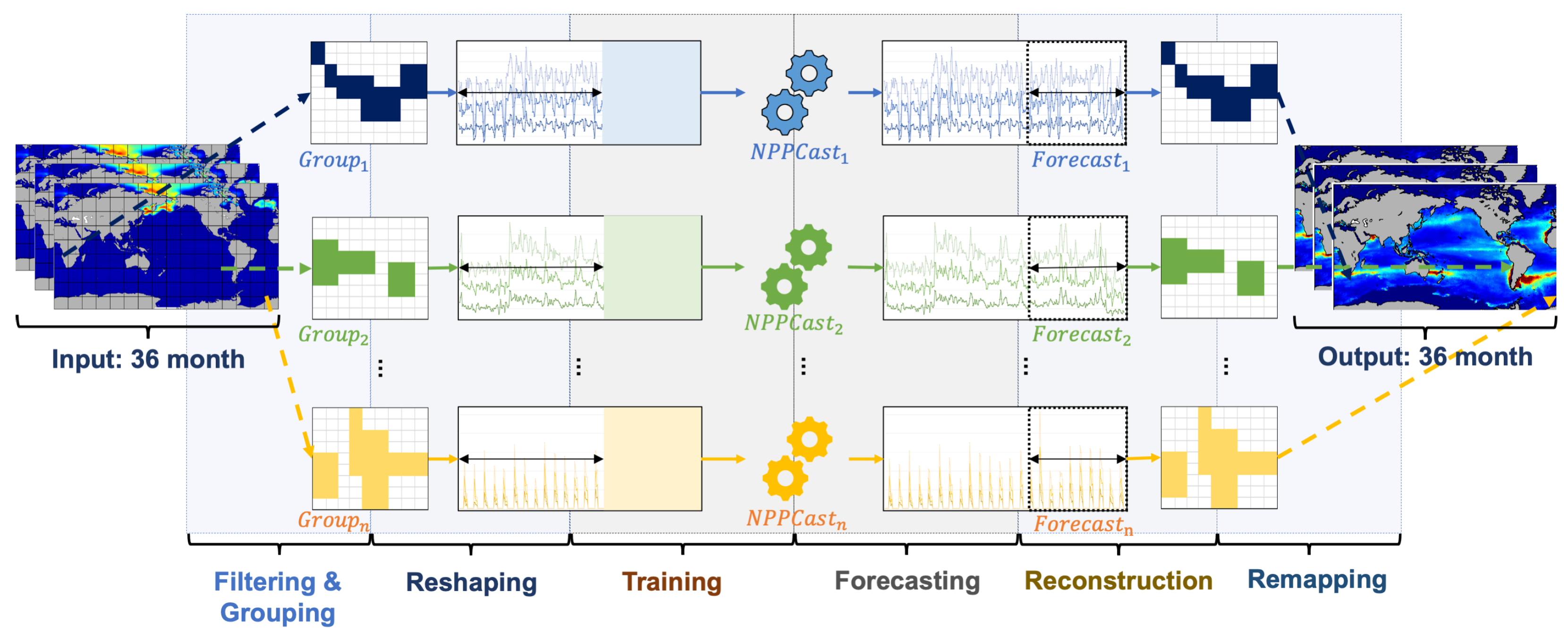
Disclaimer/Publisher’s Note: The statements, opinions and data contained in all publications are solely those of the individual author(s) and contributor(s) and not of MDPI and/or the editor(s). MDPI and/or the editor(s) disclaim responsibility for any injury to people or property resulting from any ideas, methods, instructions or products referred to in the content. |
© 2025 by the authors. Licensee MDPI, Basel, Switzerland. This article is an open access article distributed under the terms and conditions of the Creative Commons Attribution (CC BY) license (https://creativecommons.org/licenses/by/4.0/).