Application of Structure from Motion Techniques Using Historical Aerial Images, Orthomosaics, and Aerial LiDAR Point Cloud Datasets for the Investigation of Debris Flow Source Areas

Highlights

What are the main findings?

• Structure from Motion (SfM) applied to archival aerial imagery can produce reliable 3D reconstructions in complex Italian Alpine areas when supported by careful GCP placement, high-resolution scanning, and robust co-registration.
• Multi-temporal comparison with LiDAR data revealed measurable erosion and deposition patterns linked to documented debris flow events, and visual interpretation extended the reconstruction of geomorphological changes over nearly 80 years.

What are the implications of the main findings?

• Historical aerial imagery, despite variable quality, represents a valuable resource for assessing long-term sediment dynamics and landscape evolution in data-scarce mountain environments.
• Adapting SfM workflows to archival datasets enhances hazard assessment by identifying debris flow source areas and supporting sediment transfer analysis at decadal scales.

Abstract

Detecting topographic change in mountainous areas using historical aerial imagery is challenging due to complex terrain and variable data quality. This study evaluates the potential of Structure from Motion (SfM) for deriving 3D information from archival photograms in the Rabbia basin (Central Italian Alps), a catchment with a well-documented history of debris flow activity. The aim is to assess the impact of input configurations and photogrammetric processing strategies on the quality and interpretability of 3D reconstructions from historical aerial imagery, as a basis for further geomorphological analyses. A 1999 aerial dataset was processed via SfM workflow to generate a point cloud and orthomosaic, and then co-registered with a 2021 LiDAR-derived dataset. Multi-temporal analysis was conducted using point cloud distance computations and visual interpretation of orthomosaics. Additional aerial images spanning nearly 80 years expanded the temporal scale of the analysis, providing valuable retrospective insight into long-term terrain evolution. The results, although considered semi-quantitative due to data quality limitations, are consistent with geomorphological trends in the area. The study confirms that historical SfM-derived products, when supported by robust co-registration and quality checks, can contribute to sediment dynamics and hazard evaluation in alpine environments, though result interpretation should remain cautious due to dataset-specific uncertainties.

1. Introduction

Debris flows represent one of the most hazardous and unpredictable geo-hydrological processes affecting Alpine environments. Their occurrence is controlled by a complex interplay of topographic, lithological, and climatic factors [1,2,3], which complicate both their spatial prediction and magnitude estimation. These events are capable of mobilising large volumes of sediment with high energy, causing severe damage to infrastructures and human lives [4,5,6,7]. Unlike other gravitational processes, debris flow activity is not directly correlated with event frequency; a high recurrence rate does not necessarily imply sediment exhaustion [3]. Instead, the availability of mobilisable material is regulated by multiple interdependent factors [8], such as the geomorphology and connectivity of minor hydrographic networks, hydrological regime, permafrost degradation, snow/glacier melt dynamics and morain mobilisation [9,10,11,12]. Studies [13] have emphasized the critical role of small tributaries in initiating and enhancing sediment transfer during debris-flow events, acting as amplifiers of geomorphological processes.

Recent climatic trends in the Alps [14] have led to a reduction in persistent snow and glacial cover, accompanied by increased water availability [15]. Ice bodies (glaciers, permafrost and rock glaciers) provide a stabilising effect on unconsolidated slope material. Their degradation, therefore, results in reduced sediment holding capacity and an increase in potentially mobilisable debris [16,17]. The subsequent accumulation of loose debris along slopes and torrent beds increases both the potential magnitude [18,19,20,21] and the frequency of debris flow initiation, especially under increasingly frequent extreme precipitation events [22,23,24,25,26,27,28]. In steep, fractured lithological settings, intense precipitation or rapid snowmelt exacerbates slope instability, promoting the detachment and downslope transport of debris. When these sediment rich slopes are hydrologically connected to main drainage channels [29], debris flows can propagate rapidly downstream and, in some cases, reactivating pre-existing landslide bodies [17] A comprehensive understanding of sediment supply conditions requires extending the analysis beyond depositional areas and focusing on the source areas, defined as localised zones of active erosion or mass movement that contribute to the sediment budget of the basin [30]. These areas, often located along steep slopes or in active channels, can include heterogeneous surficial deposits such as glacial tills, debris accumulations and landslide remnants [31]. Given the pronounced temperature increase in Alpine regions [32,33], the reconstruction of long-term sedimentary dynamics has become a central objective in geomorphological and hazard-related studies. In this context, historical aerial imagery provides a unique opportunity for retrospective analysis [34,35,36], particularly in areas where historical visual documentation is scarce. By enabling the reconstruction of past topographic surfaces, these data sources offer valuable insights into long-term erosion/deposition trends and landscape evolution [37,38]. The photogrammetric archive hosted by the National Research Council, Research Institute for Geo-Hydrological Protection (CNR IRPI), comprises an extensive dataset of historical aerial photograms acquired over several decades across northern Italy. Traditionally employed through analogue stereoscopic analysis, these images have recently been digitised and made available via an online platform [39], facilitating broader access and the potential for quantitative 3D reconstruction. With advances in Structure from Motion (SfM), it is now possible to extract high-resolution Digital Elevation Models (DEMs) from archival imagery, enabling multi-temporal terrain analysis with decadal resolution even across extensive and complex landforms [38,40]. This approach has been applied in a wide range of geomorphological contexts, including glacier monitoring [41,42,43,44,45,46,47,48], fluvial systems [49,50,51], coastal evolution [50,52,53,54,55], landslide dynamics [38,54,56,57] and volcanic terrains [40,58].

Despite its growing application, SfM-based processing of historical imagery presents methodological challenges, particularly in high-relief alpine environments [41]. The reliability and metric accuracy of derived 3D products are strongly dependent on input data characteristics, which often include heterogeneous resolution, incomplete metadata, lack of camera calibration and radiometric inconsistencies [59,60]. Topographic complexity, combined with geometric limitations of the acquisition process, can introduce errors during 3D reconstruction, such as surface reconstruction deformations or localised distortions [35]. Challenges may arise due to heterogeneous spatial resolution and registration errors when integrating historical data with modern high-resolution datasets [38,61]. Furthermore, the final accuracy is critically influenced by scanning resolution [62], the spatial distribution and accuracy of Ground Control Points (GCPs) [37], the quality of the input images [35], possible physical damage to the images and the specific configuration of SfM software parameters [59]. Integration of datasets from different acquisition times often introduces alignment inconsistencies, limiting the accuracy of change detection and volumetric analysis. Despite the increasing adoption of SfM for geomorphological purposes, a systematic understanding of how these factors interact remains limited [35]. Because each historical dataset presents unique challenges [52,63], case-specific assessments are essential before generalising findings. Improving the reliability of SfM-derived models for long-term topographic analysis requires a deeper awareness of these methodological sensitivities, particularly in contexts demanding precise quantitative comparisons.

To fill a methodological gap in geomorphological research, this study assesses the impact of different input configurations and photogrammetric processing strategies on the quality and geomorphic interpretability of 3D models reconstructed from historical aerial imagery. An analysis of the influence of GCP characteristics, image resolution and SfM parameterization on the accuracy of point clouds was conducted. Using a representative historical dataset from a debris flow-prone basin in the Central Italian Alps (1935–2021) [64], the study assesses whether these outputs are sufficiently robust to support quantitative, multi-temporal analysis. The findings provide practical guidance for optimising SfM workflows, identifying common challenges and improving the interpretability of multi-temporal geomorphological reconstructions. In doing so, this study contributes to a broader understanding of the potential and limitations of using archival aerial imagery in terrain evolution studies.

2. Materials and Methods

2.1. Research Structure

In this study, an iterative workflow (Figure 1) was implemented to test different processing approaches and identify the optimal combination of variables for handling the historical aerial image dataset. The workflow was designed with a dual objective: (i) to generate a point cloud forming the basis of a 3D model for multi-temporal analysis, specifically through point cloud differencing over selected sub-areas; (ii) to produce orthomosaics for visual and multi-temporal comparison, and photointerpretation across the entire catchment.

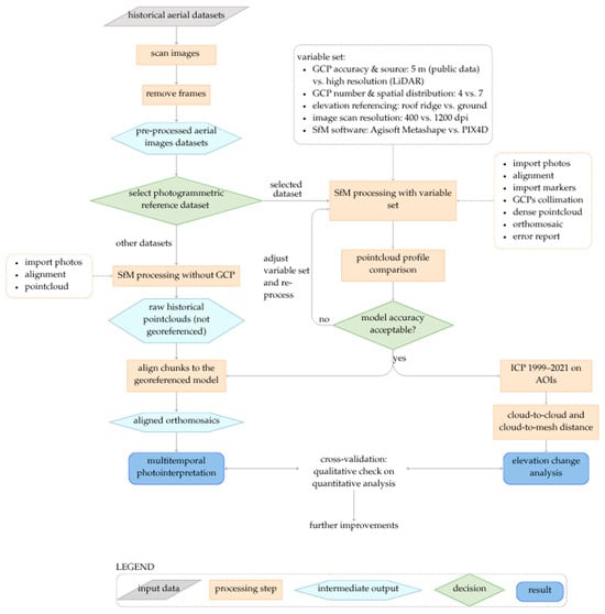
Figure 1. Flow chart of the conducted research. Iterative workflow implemented to optimise historical aerial image processing for 3D point cloud generation, orthomosaic production, and multi-temporal analysis using SfM (Agisoft Metashape Professional, 2.1.3 version, and PIX4Dmapper, 4.10.1 version), point cloud elaboration (TerraScan, 025.011 version, and CloudCompare, 2.14 version) and GIS (QGis, 3.42.2 version) tools.

Data processing consisted of several stages and required the usage of different software packages due to the diversity of source data, such as rasters, vectors and LAS formats [34]. The following software were used: Agisoft Metashape Professional (2.1.3 version) [65] and PIX4Dmapper (4.10.1 version) [66] for the SfM analysis; TerraScan (025.011 version) [67] and CloudCompare (2.14 version) for the point clouds elaborations; QGis (3.42.2 version) to combine the different layers and interpret the results.

2.2. Study Area

The Rabbia basin is located in the northern sector of the Valcamonica (Lombardy Region, Northern Italy), a major glacial-fluvial valley crossed by the Oglio River. The Rabbia catchment exhibits a fan-shaped morphology, with its geometric apex located at the confluence of the main watercourses to the west and its boundaries defined by Cima dei Laghi Gelati (3254 m a.s.l., east), Monte Aviolo (2881 m a.s.l., north) and Monte Bompià (2782 m a.s.l., south). The E–W-oriented catchment has a real surface area of 196.6 km² and includes two sub-basins: Gallinera and Rabbia (also known as Valle di Bombiano).

Geologically, the area is intersected by the Gallinera Tectonic Line and is predominantly composed of the Edolo Schist Formation, consisting mainly of mica schists and phyllites. These lithologies, part of the metamorphic crystalline basement, overlie the Southern Alpine sedimentary cover and related intrusive bodies, forming a complex tectonic structure that strongly influences slope stability and lithological variability (Figure 2). The upper basin is dominated by highly fractured bedrock [68], promoting mechanical weathering and continuous debris production [69]. Two major glacial cirques, surrounded by sharp alpine ridges, contain extensive loose debris feeding both debris flow source zones and the main drainage system [70]. Glacial deposits dominate the headwaters, where permafrost degradation and glacial retreat (below 2000 m a.s.l.) further contribute to seasonal summer discharge. While surface deposits are largely fine-grained, they frequently contain boulders up to 3.5 m in diameter and reach several meters in thickness [71]. Moraines are poorly developed, but some lobate features resembling rock glaciers are present. Surface deposits include eluvio-colluvial mantles, glacial and detrital sediments and localized gravitational accumulations. In some areas, talus slopes and debris cones are incised by active flow channels that further mobilise sediment downslope.

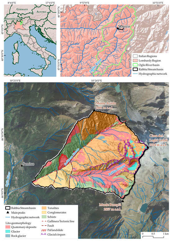
Figure 2. Main geological and geomorphological features of the Rabbia basin.

The basin exhibits intense geomorphological activity, notably marked by the Pal landslide, a large rota-translational mass movement involving approximately 12 million m³ of material [72]. This landslide affects the right bank of the Gallinera Stream and directly intersects the main river channel near the terminal section of the catchment. Following recent debris-flow events, the landslide has shown signs of renewed movement, representing a potential sediment source that could increase the magnitude of future debris flows. Documented debris flows (Table 1) underscore the high frequency and intensity of such processes. These pulse-like flows, often exceeding velocities of 10 m/s, are capable of transporting large blocks and pose significant threats to downstream communities, particularly the municipality of Sonico due to its proximity to the Oglio River confluence [71].

Table 1. Historical debris flow events in the Rabbia basin.

Year	Month	Day
1757	08	30–31
1765	07	-
1825	08	05
1828	09	13–14
1829	08	-
1839	09	02
1850	08	14–15
1869	09	11
1882	09	15
1885	-	-
1911	08	-
1952	10	26
1953	07	-
1936	08	-
1960	09	17–20
1985	08	25–26
1987	07	18
1987	08	24–25
1987	09	26
1991	07	5–6
1999	10	07
2006	10	15
2006	07	24
2006	07	31
2012	07	27
2013	10	24
2018	08	5–6
2020	08	29
2023	08	27

Given the pronounced altitudinal gradients (600–3100 m a.s.l.) that characterize the Rabbia catchment, orographic effects driven by steep slopes and valley orientation enhance condensation and promote abundant precipitation, which increases with elevation. Observations from the Camonica valley and ARPA Lombardia stations indicate ~1000 mm mean annual precipitation at the floodplain (600–800 m a.s.l., with an annual variability ±150 mm), 1200–1300 mm at ~1200 m a.s.l., and up to 1500 mm above 2000 m a.s.l., where residual glaciers, rock glaciers, perennial snowfields, and cryonival deposits occur. At these elevations, snowfall dominates in winter and sustains spring–summer runoff. Seasonality shows two maxima: localised, high-intensity thunderstorms in summer, linked to diurnal heating and orographic convection, and widespread, persistent rainfall in autumn, associated with Atlantic and Mediterranean disturbances. Winter totals are comparatively low, although solid precipitation above 1200–1400 m a.s.l. remains important for seasonal snow accumulation. Pluviometric analyses confirm the role of extremes: short-duration (1–24 h) events can reach several tens of millimeters per hour, triggering flash floods, debris flows, and slope instabilities, as observed in the upper Rabbia basin (e.g., 2023). Overall, the catchment is characterised by abundant and highly variable precipitation, strongly influenced by extreme events, which enhance its susceptibility to hydro-geomorphological hazards.

A set of sub-areas was selected for the analysis. Four distinct Areas of Interest (AoIs) were delineated based on geomorphological and sedimentological characteristics (Figure 3): (i) the Pal landslide (AoI_1); (ii) a sector of the hydrographic network located in the northern, sun-exposed portion of the catchment (AoI_2); (iii) a high-altitude zone containing glacial and debris flow deposits situated at the base of small retreating glaciers, characterised by high stream connectivity (AoI_3); (iv) an area dominated by colluvial deposits and slope debris, located downslope of active or relict rock glaciers, where evidence of intensified erosional processes is present (AoI_4). The AoIs 1 and 2 cover a real surface area of approximately 30 km² each, while areas 3 and 4 range between 65 and 70 km².

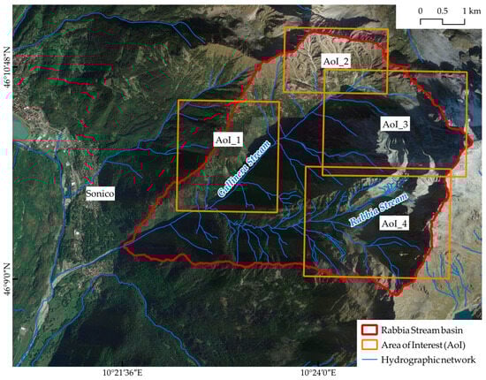
Figure 3. Selected AoIs shown in orange. Each area was selected based on its geomorphological relevance and the presence of potentially mobilisable loose debris.

2.3. Archival Imagery Datasets

Historical aerial photograms from the CNR IRPI archive [39] were reviewed and selected based on the coverage of the study area. Seven different aerial surveys were used for the analysis: 1935, 1954, 1961, 1975, 1983, 1991 and 1999 (Table 2). These datasets differ in several aspects, such as flight altitude, spatial resolution and image characteristics (e.g., panchromatic or RGB format). Following the multi-temporal SfM strategy advanced by Scaioni et al. [46], the 1999 survey was adopted as the photogrammetric reference dataset as it offered the highest spatial resolution, RGB color format and most importantly the latest available acquisition data, which enabled a more robust assessment of the accuracy and usability of the resulting 3D model by comparison with the LiDAR reference dataset.

Table 2. Photogrammetric datasets from CNR IRPI archive [39].

Date	Flight Name	Number of Selected Photograms	Flight Altitude [m]	Panchromatic or RGB
31 August 1935	F. 19 Tirano	18	5800	Panchromatic
2 October 1954	F. 19 Tirano	7	10,000	Panchromatic
27 August 1961	F. Tirano 1961	22	5200	Panchromatic
late summer 1975	Prov. Brescia 1975	14	N.D.	Panchromatic
18 September 1983	F. 19 Tirano 1981–1983	13	5700	RGB
27 July 1991	F. 19 Tirano	12	7750	Panchromatic
2 October 1999	Volo IT 2000	8	8500	RGB

2.4. Structure from Motion Iterative Processing and Workflow Optimisation

SfM combines concepts from traditional photogrammetry with modern computer vision algorithms to derive dense three-dimensional point clouds from overlapping imagery [38,73]. The technique relies on the automatic detection of invariant image features to generate tie points across multiple views. A bundle adjustment procedure then iteratively solves for both interior and exterior camera parameters [74], minimising reprojection errors. When combined with multi-temporal datasets, SfM enables the reconstruction of terrain morphology and volumetric change [61]. Accuracy and geometric stability are further improved through the integration of GCPs, which provide metric constraints and reduce systematic deformation. In this study, the processing workflow included:

• import pre-processed photograms
• image alignment (feature detection and tie-point generation)
• camera optimisation (bundle adjustment)
• GCP import and marker collimation
• dense point cloud generation
• orthomosaic creation
• error reporting and quality assessment

To obtain the most detailed 3D model from the 1999 survey, key processing variables were varied (Table 3). Comparative evaluation of the resulting point clouds against the 2021 LiDAR dataset allowed to select the configuration with the lowest RMSE and highest geometric consistency. This iterative optimization ensured that the adopted SfM model provided robust geometric accuracy for subsequent geomorphological interpretation.

Table 3. Variables used during tests.

Aspect	Variable	Value
GCP for absolute accuracy	Source and accuracy GCP and spatial distribution Elevation definition	Dataset 5 m LiDAR high-resolution 4 7 roof ridge ground
Image dpi for geometric details	Scanning resolution	400 dpi/1200 dpi
Optimisation algorithms	Software	Agisoft Metashape [52] PIX4Dmapper [53]

2.4.1. Ground Control Points

The selection of a suitable reference dataset is a critical step in the georeferencing and co-registration of historical aerial imagery, as it directly affects the spatial accuracy of multi-temporal photogrammetric analysis [47,53,60,75]. The accuracy of GCP coordinates used during SfM processing strongly depends on the quality and resolution of the chosen reference. A first georeferencing attempt was based on publicly available datasets from the Geoportal of the Lombardy Region. In this phase, planimetric coordinates were obtained from the 2018–2019 orthophoto, while vertical control was provided by a 5-m resolution DTM dated 2015, which was derived from cartographic interpolation rather than direct topographic measurements [76]. A more accurate georeferencing solution was subsequently implemented using a high-resolution LiDAR dataset acquired in 2021 by the CNR-IRPI for the Lombardy Region. This dataset included both raw ellipsoidal point clouds and orthophotos acquired during the same flight campaign. Raw data was provided as a point cloud with an average density of approximately 10 points per square meter. All reference datasets were projected using the WGS 84/UTM zone 32N coordinate system (EPSG:32632). The use of LiDAR-derived products for validating and supporting three-dimensional model generation through SfM techniques is well established. Several studies (e.g., [53,54,77,78,79]) have demonstrated the effectiveness of high-resolution LiDAR point clouds as reliable elevation references or “ground truth”, particularly in remote or inaccessible mountainous environments.

Between 4 and 7 GCPs were identified (Figure 4), positioned around the catchment perimeter from valley floor to ridge crest [80], in order to maximise geometric stability while avoiding features altered after 1999 (e.g., the rebuilt fan-bridge). GCPs were required to be stable, easily identifiable in both datasets and visible in ≥3 images. Points showing large residuals were disabled before the final bundle adjustment.

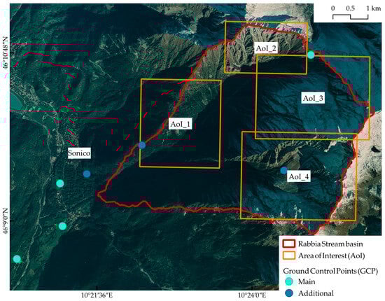
Figure 4. Spatial distribution of GCPs used for the co-registration of the 1999 dataset. Light blue markers indicate the points employed in the 4GCP tests, while dark blue markers represent the additional GCPs used in the 7GCP test.

For GCPs at building corners, elevation was assigned either to the roof ridge or the ground-level intersection with the LiDAR point cloud (ground). The effect on vertical accuracy was evaluated.

2.4.2. Scanning Resolution

The original analogue aerial photograms were initially processed using existing digital versions scanned at the maximum available resolution of 400 dpi with a Fujitsu fi-6770 (Fujitsu, PFU Limited, Kahoku, Japan) device. However, due to the limited spatial detail and the inadequacy of the resulting photogrammetric products, the same frames were subsequently re-scanned at 1200 dpi in TIFF format using a Colortrac SmartLF SC 42 Xpress scanner (Colortrac, St Ives, United Kingdom), non-photogrammetric, to enhance image quality and support more accurate 3D reconstruction. As suggested by Seccaroni et al. [81], the optimal scanning resolution for photogrammetric applications typically ranges between 800 and 1600 dpi to preserve geometric fidelity. A 24-bit RGB color mode was applied during scanning, as it produced superior visual and radiometric quality compared to the alternative configurations available on the scanning software. However, as noted by Rault et al. [80], raw scanned images cannot be directly used in SfM workflows due to geometric distortions and non-image content such as borders or fiducial marks. Therefore, a preprocessing step was required prior to photogrammetric reconstruction. This included the removal of image borders and standardisation of the image layout. The goal of this preprocessing phase was to ensure optimal input quality for SfM reconstruction and to facilitate the generation of accurate and dense 3D point clouds [32].

Both Agisoft Metashape and PIX4Dmapper were run with comparable settings (with the “highest” quality level applied to both image alignment and dense point cloud generation), as different matching algorithms may affect results [41,82,83]. PIX4Dmapper tests also included Manual Tie Points (MTPs) to enhance the alignment.

The resulting best dense point cloud was exported in LAS format for downstream analyses and formed the basis for other historical datasets alignment.

2.5. Cloud-to-Cloud and Cloud-to-Mesh Distances Between 1999 and 2021 on Areas of Interest

Multi-temporal terrain change was estimated by differencing successive three-dimensional datasets, following the cloud-to-cloud (C2C) and cloud-to-mesh (C2M) approach widely applied in SfM studies (e.g., [60,74,84,85]). Analyses were restricted to the four previously defined AoIs in order to focus on the most active sediment-source areas. The 1999 SfM-derived point cloud, processed as described in Section 2.4, was compared with the 2021 LiDAR point cloud, which served as the reference geometry. Both clouds were first clipped in TerraScan to identical extents and then co-registered in CloudCompare using the Iterative Closest Point (ICP) algorithm, thereby removing residual rigid offsets over presumed stable terrain [86]. Three distance metrics were computed: (i) absolute C2C distance with a 25 m search radius, (ii) absolute C2C distance with a 10 m radius for finer detail, and (iii) a C2M comparison at 10 m in which the 1999 cloud was evaluated against a triangulated mesh of the 2021 LiDAR surface. Only the C2M output provides signed values, allowing direct interpretation of negative distances as erosion and positive distances as deposition, whereas the two C2C products quantify the magnitude of surface change over the years, as they do not capture the directionality.

2.6. Qualitative Analysis

For the visual component of the multi-temporal analysis, all available aerial photogrammetric datasets covering the full extent of the study area were considered. Each dataset was processed through an SfM workflow without GCPs, with the objective of generating point clouds in a local reference system, both in Agisoft Metashape and PIX4Dmapper. Once the raw point clouds were produced, they were aligned to the georeferenced 1999 dataset using the Align Chunks function in Agisoft Metashape [48,81], setting the “point-based” option. This approach allows for the relative co-registration of other datasets without the need for independent georeferencing of each image block, streamlining the workflow and reducing manual input [81]. The sequence of co-aligned orthomosaics enables the visual assessment of geomorphological changes through interpretation, facilitating the identification of geomorphological features and processes over time.

3. Results

3.1. SfM Reconstruction of the 1999 Survey

The 1999 aerial survey was first processed using 400 dpi scans, which proved inadequate due to large planimetric and altimetric errors (total RMSE = 277 m). Re-scanning the images at 1200 dpi improved tie point detection and vertical detail, enabling a more reliable elevation model. However, while the 1200 dpi re-scan improved overall image quality, it also revealed underlying defects in the original digital frames, such as striping artefacts inherited from the earlier 400 dpi scan, and new scanning-related issues, including isolated saturated pixels likely caused by sensor anomalies in the scanner itself. These defects manifested as outliers in elevation profiles, affecting the reliability of the 3D reconstruction. In addition, two photograms were excluded from the bundle adjustment due to insufficient tie point quality, further reducing the usable image block and affecting spatial coverage.

The study area’s steep and heterogeneous terrain, including vegetation and snow cover, limited the availability of suitable GCPs. Three configurations using different GCP accuracies, elevation references and numbers of points were tested in Agisoft Metashape [65], all using 1200 dpi imagery and LiDAR-derived XYZ coordinates (Table 4). The three models tested include: the 4_r model using 4 GCPs referenced to roof ridges, the 4_g model using 4 GCPs referenced to ground level, and the 7_g model using 7 GCPs referenced to ground level.

Table 4. Error statistics from the three Metashape processing tests using different GCP configurations. The values represent the root mean square error (RMSE) in the X, Y, XY and Z directions, as well as the total 3D error, all expressed in meters.

Point Cloud Name	GCP Number	Elevation Referencing	X Error (m)	Y Error (m)	Z Error (m)	XY Error (m)	Total RMSE (m)
4_r	4	Roof ridge	0.58	1.5	2.23	1.61	2.76
4_g	4	Ground	0.36	1.37	2.06	1.41	2.51
7_g	7	Ground	0.73	0.89	1.71	1.16	2.07

As shown by the error report (Table 4), the 7_g model achieved the lowest total RMSE (2.07 m) and, therefore, the highest metric accuracy. To further validate this result, a verification was carried out through the comparison of point cloud cross-sections from the 1999 datasets and the 2021 LiDAR reference along selected cross-sections. Three cross-sections were analysed (Figure 5): transect A-A′ crossing the watershed divide, transect B-B′ in the valley floor section, and transect C-C′ in the upper catchment area. Due to the low density of the 1999 point clouds, interpolated elevation profiles (e.g., via CloudCompare) produced visually misleading artefacts. Therefore, a visualisation of raw point profiles using Terrascan was performed (Figure 6 and Figure 7), which provides a more faithful representation of the actual terrain morphology and better supports the comparison between datasets.

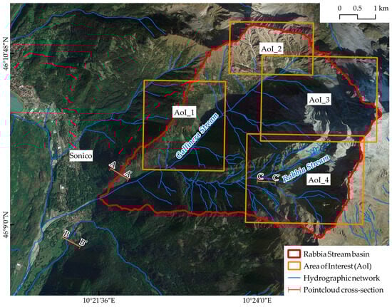
Figure 5. Cross-sections were analysed to assess discrepancies between SfM-derived point clouds and the 2021 LiDAR-based point cloud.

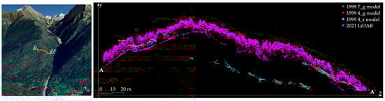
Figure 6. Point cloud profile comparison between the 1999 SfM-derived point clouds and the 2021 LiDAR dataset along transect A-A′ in Figure 5.

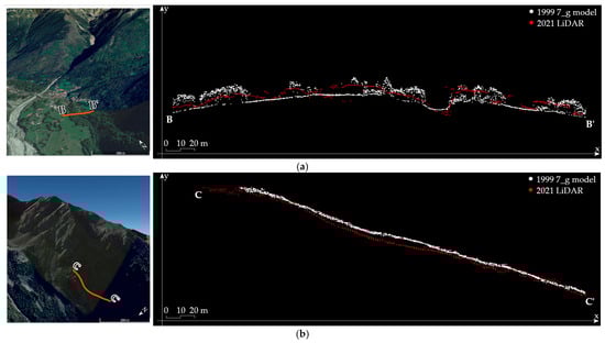
Figure 7. Comparison between the 1999 SfM-derived point cloud 7_g model (in red) and the 2021 LiDAR-derived point cloud (in white) within TerraScan, along selected cross-sections. (a) Valley floor section characterised by the presence of trees, buildings or other anthropogenic elements, representing semi-DSM conditions (transect B-B’ in Figure 5); (b) Upper catchment area over bare rock, representing semi-DTM conditions (transect C-C′ in Figure 5). The average point-to-point distance between the two-point clouds in the valley floor (a) is approximately 2 m, consistent with the overall RMSE of the 7_g model.

The point cloud comparison along transect A-A′ (Figure 6) reveals that the 7_g model (green) most closely follows the terrain morphology delineated by the 2021 LiDAR point cloud (pink), aligning with canopy tops. The other two models, 4_g (red) and 4_r (light blue), exhibit a generally parallel trend with constant vertical offsets in some sections, while deviating more substantially in others. The 7_g model demonstrated higher accuracy on sloped terrains compared to flat areas. Specifically, improved surface reconstruction was observed on vegetated slopes and rocky outcrops where no anthropogenic structures were present. Conversely, flat regions exhibited reduced accuracy, likely due to challenges in identifying reliable elevation points during SfM processing. Surface morphology significantly influenced model behaviour and accuracy. In vegetated areas, the 1999 7_g profile generally matches the canopy surface defined by the 2021 LiDAR point cloud, consistent with semi-DSM (Digital Surface Model) characteristics, yet captures detailed morphology at slope discontinuities. This is particularly evident along transect B-B′ in the valley floor (Figure 7a), where the point-to-point distance between the 1999 7_g model (red) and the 2021 LiDAR point cloud (white) was approximately 2 m, consistent with the overall RMSE of the 7_g model. In contrast, areas of exposed bedrock showed different behaviour. Along transect C-C′ in the upper catchment area (Figure 7b), the model operates under semi-DTM conditions over bare rock surfaces. The 7_g model approaches near-ground surfaces, and the discrepancies between the two point clouds were considerably smaller compared to vegetated areas. In these conditions, minor differences may be interpreted as measurable geomorphic changes related to erosion or deposition processes occurring between 1999 and 2021.

Despite these promising results, terrain reconstruction proved challenging in densely vegetated and shadowed areas, such as the terminal section of the Rabbia Valley, where the model produced unsatisfactory results. Similarly, in sunlit areas with dense vegetation on steep slopes, such as the Pal landslide, the model struggled to accurately reconstruct topography, highlighting the dominant influence of vegetation cover in hindering reliable elevation detection.

To assess the robustness of the workflow, the same parameters used in the 7_g Metashape test were applied in PIX4Dmapper. Despite the addition of multiple Manual Tie Points (MTPs), the automatic alignment failed to yield acceptable results, resulting in a final RMSE of 6.78 m.

3.2. Terrain Elevation Change Analysis Between 1999 and 2021 Point Clouds

The terrain elevation change analysis using C2C and C2M distances produced variable results across the selected AoIs, reflecting both terrain complexity and dataset limitations. In AoI_1, corresponding to the Pal landslide sector, the analysis failed due to the presence of dense vegetation, which resulted in large voids in the 1999 point cloud. In AoI_2, the 1999 model points were concentrated almost exclusively along the hydrological network, leaving the adjacent riverbanks, which are critical for assessing erosion dynamics, largely unrepresented. As a result, only C2C distance analysis was performed, while no mesh was generated for the 2021 dataset in this sector, as generating a mesh for the 2021 dataset and comparing it to the 1999 point cloud would have resulted in unreliable geometry. AoI_3 provided the most interpretable and meaningful dataset, particularly in high-altitude areas (Figure 8). In AoI_3, the C2M distance analysis was effective in highlighting erosion and sediment redistribution processes with sufficient clarity. In AoI_4, the computed distances were also satisfactory, although the model failed to fully capture the extent of accelerated erosion processes clearly visible through photointerpretation.

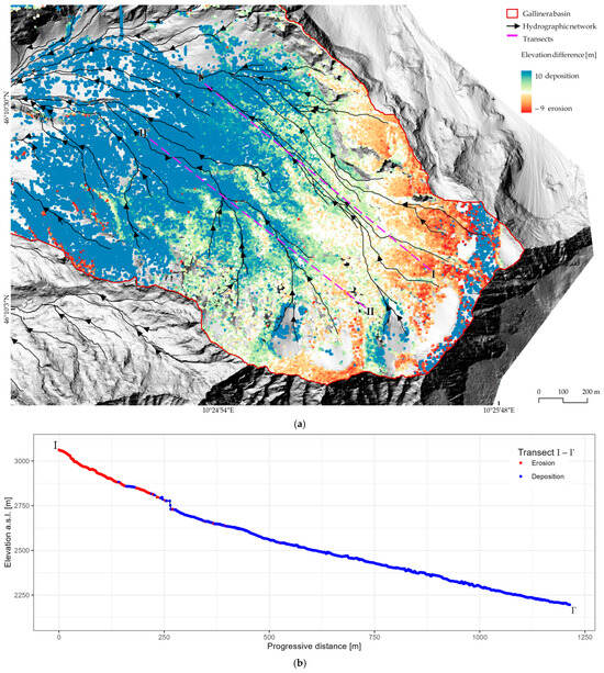
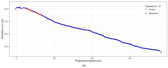
Figure 8. Cloud-to-mesh result on a subset of AoI_3 (a). The color scale ranges from red to blue, with red indicating erosion (negative values) and blue indicating deposition (positive values). Data have been clipped on a specific subset for a better visualisation of the results. The blue dots under the crests represent deposits associated with pseudo-planes, slope breaks, and double crests. The areas marked with red dots along the stream network indicate significant changes in the channel bed, referring to deepening of the riverbed. No-data regions correspond to shaded or vegetated areas, as well as continuous glacial cover at higher elevations. Distinct erosion and sediment accumulation processes are visible in the area downslope of the glacial cirques. Two cross-sections were identified on the slope examined: (b) profile I-I′, with prevalent erosion in the upper section, and (c) profile II-II′, along which deposition sectors prevail. The background hillshade is derived from the high-resolution 2021 LiDAR survey.

The analysis made it possible to identify, with sufficient detail, the slope sectors where erosional features prevail, often corresponding to flow paths along which debris mobilization processes occur, and those characterized mainly by deposition, corresponding to slope-reduction areas that favour the temporary accumulation of debris. The transects I–I′ and II–II′, developed for the sector corresponding to AoI_3 on the left slope of the Gallinera Stream (Figure 8), provide detailed evidence of the geomorphological erosion and deposition processes, which are particularly significant in terms of potential debris-flow generation.

3.3. Orthomosaic Alignment and Visual Photointerpretation

Orthomosaics were generated for all historical datasets to support a qualitative multi-temporal assessment. Prior to orthomosaic creation, individual chunks in Agisoft Metashape were aligned so that several point cloud blocks could be co-registered with the georeferenced 1999 dataset. This alignment succeeded for the 1961 and 1991 imagery, whereas the remaining datasets were mosaicked in local coordinates only. The orthomosaics displayed evident artefacts and distortions that degrade both metric accuracy and visual interpretation.

Visual photo-interpretation allows for the recognition of both past and ongoing geomorphological processes over a timespan of approximately 80 years. During interpretation, attention has been paid to the seasonality of photogrammetric acquisitions, which typically took place in summer or late summer (between July and October). This temporal variability introduces slight differences in vegetation appearance and in the extent of snow cover at higher elevations.

Within AoI_1, the Pal landslide, the 80-year image sequence reveals progressive vegetation expansion that partly masks the main scarp, while only minor variations in bank erosion are observable (Figure 9). In AoI_2, several tributaries have widened through time, pointing to an increasing flux of sediment towards the main channel (Figure 10). AoI_3 documents a steady reduction in glaciers accompanied by enhanced deposition of debris into the channel, evidencing a coupled process of erosion and deposition that mirrors the semi-quantitative analyses for this sector (Figure 11). Additional tributaries on the left side of the Gallinera catchment display intensified debris production and the persistence of seasonal snow bridges; their water content represents a latent hazard if associated with high temperatures or even low-intensity rainfall [87], potentially triggering or contributing to debris flows initiation. In AoI_4, pronounced accelerated erosion landforms appear in the central section of unconsolidated material below former cirque glaciers, together with features interpretable as active or relict rock glaciers (Figure 12). The severity of erosion varies over time, broadly matching the documented chronology of debris flow activity. It should be noted, however, that not every image set affords ideal conditions for detailed interpretation: shadows, seasonal snow cover and a high-flying altitude limit the resolution and clarity of some datasets.

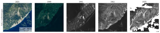
Figure 9. Detailed views of the orthomosaics generated from the different datasets over AoI_1, corresponding to the Pal landslide, and a view of the 2021 LiDAR-derived orthoimage.

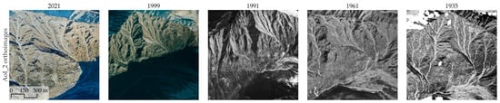
Figure 10. Detailed views of the orthomosaics generated from the different datasets over AoI_2 and a view of the 2021 LiDAR-derived orthoimage.

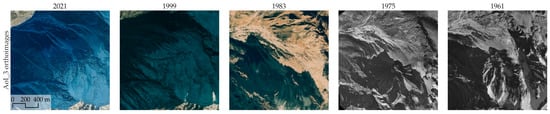
Figure 11. Detailed views of the orthomosaics generated from the different datasets over AoI_3 and a view of the 2021 LiDAR-derived orthoimage.

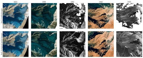
Figure 12. Detailed views of the orthomosaics generated from the different datasets over AoI_4, compared with the original aerial frame, and a view of the 2021 LiDAR-derived orthoimage. Note the presence of linear artefacts and no-data areas in the orthomosaic reconstruction.

4. Discussion

This study assessed the potential of archival aerial imagery processed with SfM to detect geomorphological processes in mountainous environments, using the Rabbia catchment as a case study. The analysis focused primarily on a 1999 photogrammetric reference dataset, implementing the full processing workflow and including additional historical datasets to support visual interpretation and extend the time scale. Despite inherent limitations, the SfM workflow produced usable terrain models from the 1999 imagery, particularly within selected AoIs. The best-performing point cloud, corresponding to the 7_g model, was validated by comparison with the 2021 LiDAR point cloud. Model accuracy proved highly sensitive to terrain morphology, as expected in mountainous settings. It is worth noting that, unlike findings in other studies where flatter areas typically yield higher accuracy (e.g., [41,77,88,89]), the model in this case performed better on sloped terrains than on presumed stable flat areas. This discrepancy is likely due to the difficulty of the model in identifying reliable altimetric points in flat zones where elevation variation is minimal. Conversely, in sloped natural environments (e.g., vegetated slopes and exposed rock), greater topographic variability and absence of anthropogenic features allowed more accurate surface reconstruction.

Although the subset of seven spatially distributed GCPs used in the best-performing model provided improved accuracy and effective geometric constraints, the overall availability of stable GCPs across the study area was limited. While low-elevation buildings provided initial horizontal control, vertical constraint was insufficient, necessitating the inclusion of stable, high-elevation rock outcrops as GCPs to improve vertical accuracy [67]. These features were selected when distinguishable in multiple datasets, either as clearly recognisable rocky surfaces or as natural landforms such as rock dihedrals, ridges, and other sharp morphologies contrasting with the surrounding pixels. The findings reinforce that GCP quality and appropriate placement are more critical than quantity alone, consistent with previous studies [90]. Given the scarcity of stable features in steep terrain, prior field knowledge remains essential to identify robust GCP locations, as minor planimetric displacements can induce vertical errors, affecting volumetric analyses [52,91]. Detailed reconstruction was achieved mainly where GCP geometry effectively constrained the model [41,53]. Despite satisfactory horizontal accuracy, localised vertical artefacts persisted, leading to exclusion of offset areas from further analyses as reconstruction errors, underscoring the importance of distinguishing real topographic changes from reconstruction noise [51].

The quality of the scanned photograms influenced all workflow stages. Although the original stereo prints appeared sharp, scanning at 400 dpi caused physical damage to the film, introducing linear defects, while the subsequent 1200 dpi rescans, despite improving image resolution, revealed saturated pixels that degraded image fidelity and introduced artefacts into the photogrammetric reconstruction [35,92]. The scanning artefacts and physical damage encountered in this case are common issues in archival aerial imagery (e.g., [43,93]) and may similarly affect other researchers relying on historical photogrammetric archives [58,94]. Additional challenges included the reduced number of available images, the low frame overlap, the limited viewing geometry and the extensive topographic shadowing, hindering tie point extraction especially in low-texture or high-parallax areas [80,84]. The exclusion of images with poor tie point quality further reduced usable coverage, exacerbated by initially limited overlap and the removal of frames. Consequently, the final image block had limited coverage in some sectors, reducing local resolution and accuracy. However, the SfM algorithm extracted sufficient tie points under strict quality thresholds [80], though typical artefacts such as spikes, no-data/voids and smoothed or blurred surfaces persisted [34,52,84].

A two-step co-registration procedure enhanced comparability across observation periods. Initial SfM alignment using GCPs was further refined by ICP alignment to the 2021 LiDAR dataset, providing a finer alignment of the previously roughly registered point clouds [91]. Accurate co-registration is essential when comparing datasets of varying quality and origin [95], particularly in complex terrain. The 20-year interval between 1999 and 2021 captured topographic changes related to several debris flow events, including the major 2012 event and the 2006 and 2020 events. Elevation changes in debris flow-prone sectors aligned with event chronology (Table 1), illustrating the utility of C2M analysis for reconstructing sediment transport and deposition. The most reliable reconstruction was in AoI_3, likely due to effective GCP placement, highlighting once again the critical role of high-quality, spatially distributed control. However, numerical values should be interpreted cautiously [96]. Due to inherent uncertainties, results are considered semi-quantitative, serving primarily to support and reinforce the qualitative photointerpretation of geomorphological processes. Referring to Figure 8, cloud-to-mesh distances reveal a consistent erosion–deposition pattern, with negative values in source areas and positive values downslope, reflecting sediment redistribution along the hydrographic network. While this overall trend matches the expected behaviour of debris flows, localised depositional signals are also evident at high elevations. These are related to glacial and periglacial settings, where counter-slopes, glacial cirques, and slope breaks favour sediment accumulation before subsequent remobilisation downslope. Field surveys and helicopter reconnaissance after the 2023 event (Figure 13) documented debris accumulations and depositional features near glacier margins, further supporting this interpretation. Although the 2023 event falls outside the analysis temporal scale, its processes are analogous to past ones, highlighting the acceleration of debris flow activity in the upper catchment. Long-term degradation of glaciated areas has exposed large depositional bodies at high elevations, already evident in headwater incisions. As a result, torrent channels can generate substantial debris flows (e.g., 2023), often initiated from steep sub-vertical rock slopes with poor geomechanical conditions extending across watershed divides. The increasing frequency of such events over the past three decades underlines the geo-hydrological criticality of high-altitude Alpine sectors (see Table 1). Overall, the co-occurrence of erosion and deposition is well captured and consistent with geomorphological interpretation, confirming the potential of multi-temporal photogrammetry for hazard assessment in rapidly evolving Alpine environments [4,97].

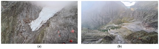
Figure 13. Post-event 2023 helicopter survey (CNR IRPI-Lombardy Region monitoring project) of the Gallinera headwater area, located in AoI_3. (a) Debris accumulation at the terminus of the retreating glacial body, exposing depositional units to precipitation and subglacial flow. (b) Upstream-to-downstream view showing the coupling of erosive and depositional processes.

While SfM-derived point clouds do not reach LiDAR-level accuracy, they provide valuable historical topographic information when higher-resolution data are unavailable [80]. Qualitative interpretation of co-registered orthomosaics, supported by visual inspection of original imagery, was essential to contextualise quantitative surface change results. Although orthomosaics were generated for all processed datasets, only two were successfully automatically co-registered to the 2021 reference, limiting subsequent quantitative analysis to these co-aligned mosaics. The difficulties encountered mirror those already noted for the quantitative analysis. While the orthorectification is technically reliable, geometric distortions in some orthomosaics reduced the visual definition of geomorphic features, limiting their usefulness for detailed interpretation and making direct inspection of the original frames preferable. Despite these limitations, the ability to retrospectively analyse terrain evolution over nearly 80 years for the Rabbia basin represents a remarkable contribution to long-term geomorphological research (Figure 14).

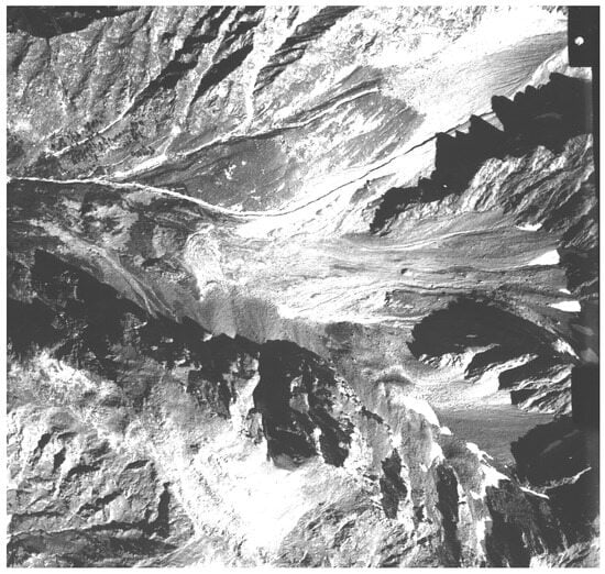
Figure 14. Detail of a rare 1935 aerial image [39] over AoI_4, showing debris flow levees, incisions, exposed depositional bodies, perennial snowfields, cryonival deposits and rock glacier features in the upper Rabbia basin. The image supports qualitative geomorphological interpretation, while further work is needed before quantitative analysis can be performed.

Although advances in SfM automation have been made, full automation remains a future challenge for historical data [93,98]. Archival datasets vary widely in scale, resolution and quality, requiring manual processing and case-specific adjustments [52,63,84]. One of the most critical steps is image pre-processing, often required to adapt scanned historical images for SfM [99]. To address this, some authors have proposed methodologies to automate the workflow or specific steps of the process (e.g., [47,100,101,102]). However, a standardised framework is still needed to improve reproducibility and comparability across studies, as highlighted by recent literature [84,97,103,104].

5. Conclusions

This study demonstrated that, despite challenges posed by archival image quality, complex terrain and limited GCP availability, a reliable 1999 point cloud was successfully reconstructed in selected areas. ICP alignment enhanced the geometric consistency, enabling semi-quantitative and multi-temporal comparisons. Detected point cloud distances revealed measurable erosion and deposition patterns consistent with known debris flow events. Qualitative orthomosaic interpretation further supported the identification of geomorphological changes and terrain evolution over nearly 80 years, although some image distortions limited their utility.

The main contribution lies in adapting modern SfM workflows to archival aerial data in high-relief, data-scarce alpine environments, highlighting critical factors such as high-resolution image scanning, appropriate GCP distribution and iterative processing to mitigate errors from parallax and low texture. Despite practical constraints from non-photogrammetric scans, meaningful 3D reconstructions and change detection were attained, validating the approach with appropriate checks. This approach, building on established methods, provides a reproducible framework for selecting the most appropriate processing strategy given a dataset with specific limitations.

Future work will focus on rescanning the 1999 photograms with dedicated photogrammetric scanners to improve resolution and reduce scanning artifacts, extending this approach to other historical datasets to broaden temporal coverage and enhance understanding of long-term geomorphological dynamics. The spatial patterns of signed C2M distances demonstrated here provide initial insights into erosion–deposition processes, and the current contribution establishes a foundation for subsequent research. Future analyses will use these SfM-derived elaborations to quantify sediment budgets, evaluate debris flow connectivity, and track long-term landscape evolution, supporting robust geomorphological interpretation and hazard assessment. Further work should also aim to quantify geomorphic displacements and estimate erosion and deposition volumes using forthcoming high-resolution data, to be acquired through a planned LiDAR survey. This will enable robust DEM of Difference (DoD) analyses for recent time periods, supporting sediment budgeting assessment and the evaluation of check dam effectiveness [97,105].

Retrospective SfM analysis using archival aerial imagery offers a cost-effective and valuable tool for long-term geomorphological analyses and hazard assessment in mountainous regions with limited high-resolution data, enhancing the value of existing historical datasets. Indeed, these datasets are already archived and accessible, though requiring careful adaptation to ensure their reliability for such analyses. Moreover, applying SfM to archival imagery enhances understanding of slope evolution by identifying debris flow source areas and delineating zones of increased hydrogeological risk, supporting sediment transfer tracking over decadal timescales. The findings provide guidance for developing reproducible workflows applicable to similarly challenging environments.

References

- Hungr, O.; McDougall, S.; Bovis, M. Entrainment of material by debris flows. In Debris-Flow Hazards and Related Phenomena; Jakob, M., Hungr, O., Eds.; Springer: Berlin/Heidelberg, Germany, 2005; pp. 135–158. [Google Scholar] [CrossRef]
- Ballesteros-Cánovas, J.A.; Stoffel, M.; de Haas, T.; Bodoque, J.M. Debris flow dating and magnitude reconstruction. In Ad-vances in Debris-flow Science and Practice; Jakob, M., McDougall, S., Santi, P., Eds.; Geoenvironmental Disaster Reduction; Springer International Publishing: Cham, Switzerland, 2024; pp. 219–248. [Google Scholar] [CrossRef]
- de Haas, T.; Lau, C.-A.; Ventra, D. Debris-flow watersheds and fans: Morphology, sedimentology and dynamics. In Advances in Debris-flow Science and Practice; Jakob, M., McDougall, S., Santi, P., Eds.; Geoenvironmental Disaster Reduction; Springer International Publishing: Cham, Germany, 2024; pp. 9–74. [Google Scholar] [CrossRef]
- Blasone, G.; Cavalli, M.; Marchi, L.; Cazorsi, F. Monitoring sediment source areas in a debris-flow catchment using terrestrial laser scanning. CATENA 2014, 123, 23–36. [Google Scholar] [CrossRef]
- Turconi, L.; Voglino, B.; Savio, G.; Tropeano, D.; Bono, B.; Luino, F. Debris flow susceptibility in a touristic alpine area: The case study of the Bardonecchia town (Upper Susa Valley, NW Italy). J. Maps 2025, 21, 2555342. [Google Scholar] [CrossRef]
- He, S.; Jiang, Y.; Ji, X. Review on the economic loss of debris flow disaster. Disasterology 2019, 34, 153–158. [Google Scholar]
- Chen, J. Research on Dynamic Risk Assessment of Debris Flow Disaster Induced by Extreme Rainfall in Mountainous Areas. Master’s Thesis, Northeast Normal University, Changchun, China, 2019. [Google Scholar]
- Tropeano, D.; Turconi, L. Geomorphic classification of alpine catchments for debris-flow hazard reduction. In Proceedings of the Debris-Flow Hazards Mitigation: Mechanics, Prediction and Assessment, Davos, Switzerland, 10–12 September 2003; Chen, C.L., Ed.; Millpress Science Publishers: Rotterdam, The Netherlands, 2003; pp. 1221–1232, ISBN 90-77017-78-X. [Google Scholar]
- Boeckli, L.; Brenning, A.; Gruber, S.; Noetzli, J. Permafrost distribution in the European Alps: Calculation and evaluation of an index map and summary statistics. Cryosphere 2012, 6, 807–820. [Google Scholar] [CrossRef]
- Nigrelli, G.; Chiarle, M. 1991–2020 climate normal in the European Alps: Focus on high-elevation environments. J. Mt. Sci. 2023, 20, 2149–2163. [Google Scholar] [CrossRef]
- Bosso, D.; Nigrelli, G.; Turconi, L.; Chiarle, M. Colate detritiche in alta quota nelle Alpi Italiane in un contesto di cambiamento climatico e degradazione della criosfera. In Proceedings of the I Fenomeni D’instabilità Naturale in Alta Montagna. La Colata Detritica del 13 Agosto 2023 a Bardonecchia: Previsione, Prevenzione e Mitigazione dei Processi (In Italian), Bardonecchia, Italy, 20–21 June 2024. [Google Scholar]
- Nigrelli, G.; Paranunzio, R.; Turconi, L.; Luino, F.; Mortara, G.; Guerini, M.; Giardino, M.; Chiarle, M. First national inventory of high-elevation mass movements in the Italian Alps. Comput. Geosci. 2024, 184, 105520. [Google Scholar] [CrossRef]
- Turconi, L.; Tropeano, D.; Savio, G.; Bono, B.; De, S.K.; Frasca, M.; Luino, F. Torrential hazard prevention in alpine small basin through historical, empirical and geomorphological cross analysis in NW Italy. Land 2022, 11, 699. [Google Scholar] [CrossRef]
- Jacob, D.; Petersen, J.; Eggert, B.; Alias, A.; Christensen, O.B.; Bouwer, L.M.; Braun, A.; Colette, A.; Déqué, M.; Georgievski, G.; et al. EURO-CORDEX: New high-resolution climate change projections for European impact research. Reg. Environ. Change 2013, 14, 563–578. [Google Scholar] [CrossRef]
- Stoffel, M.; Allen, S.K.; Ballesteros-Cánovas, J.A.; Jakob, M.; Oakley, N. Climate change effects on debris flow. In Advances in Debris-Flow Science and Practice; Jakob, M., McDougall, S., Santi, P., Eds.; Geoenvironmental Disaster Reduction; Springer International Publishing: Cham, Germany, 2024; pp. 273–308. [Google Scholar] [CrossRef]
- Kofler, C.; Mair, V.; Gruber, S.; Todisco, M.C.; Nettleton, I.; Steger, S.; Zebisch, M.; Schneiderbauer, S.; Comiti, F. When do rock glacier fronts fail? Insights from two case studies in South Tyrol (Italian Alps). Earth Surf. Proc. Landf. 2021, 46, 1311–1327. [Google Scholar] [CrossRef]
- Kang, C.; Imaizumi, F.; Theule, J. Sediment entrainment and deposition. In Advances in Debris-Flow Science and Practice; Jakob, M., McDougall, S., Santi, P., Eds.; Geoenvironmental Disaster Reduction; Springer International Publishing: Cham, Germany, 2024; pp. 165–190. [Google Scholar] [CrossRef]
- Stoffel, M.; Mendlik, T.; Schneuwly-Bollschweiler, M.; Gobiet, A. Possible impacts of climate change on debris-flow activity in the Swiss Alps. Clim. Change 2014, 122, 141–155. [Google Scholar] [CrossRef]
- Liu, W.; He, S. Comprehensive modelling of runoff-generated debris flow from formation to propagation in a catchment. Landslides 2020, 17, 1529–1544. [Google Scholar] [CrossRef]
- Chiarle, M.; Geertsema, M.; Mortara, G.; Clague, J.J. Relations between climate change and mass movement: Perspectives from the Canadian Cordillera and the European Alps. Glob. Planet. Change 2021, 202, 103499. [Google Scholar] [CrossRef]
- Jacquemart, M.; Weber, S.; Chiarle, M.; Chmiel, M.; Cicoira, A.; Corona, C.; Eckert, N.; Gaume, J.; Giacona, F.; Hirschberg, J.; et al. Detecting the impact of climate change on alpine mass movements in observational records from the European Alps. Earth-Sci. Rev. 2024, 258, 104886. [Google Scholar] [CrossRef]
- Stoffel, M.; Conus, D.; Grichting, M.A.; Lièvre, I.; Maître, G. Unraveling the patterns of late Holocene debris-flow activity on a cone in the Swiss Alps: Chronology, environment and implications for the future. Glob. Planet. Change 2008, 60, 222–234. [Google Scholar] [CrossRef]
- Messmer, M.; Simmonds, I. Global analysis of cyclone-induced compound precipitation and wind extreme events. Weather. Clim. Extremes 2021, 32, 100324. [Google Scholar] [CrossRef]
- Tuel, O.; Martius, A. A climatology of sub-seasonal temporal clustering of extreme precipitation in Switzerland and its impacts. Hydrol. Earth Syst. Sci. 2021, 21, 2949–2972. [Google Scholar] [CrossRef]
- Lehmann, J.; Coumou, D.; Frieler, K. Increased record-breaking precipitation events under global warming. Clim. Change 2015, 132, 517–518. [Google Scholar] [CrossRef]
- Rädler, A.T.; Groenemeijer, P.H.; Faust, E.; Sausen, R.; Púčik, T. Frequency of severe thunderstorms across Europe expected to increase in the 21st century due to rising instability. npj Clim. Atmos. Sci. 2019, 2, 30. [Google Scholar] [CrossRef]
- Kahraman, A.; Kendon, E.J.; Chan, S.C.; Fowler, H.J. Quasi-stationary intense rainstorms spread across Europe under climate change. Geophys. Res. Lett. 2021, 48, e2020GL092361. [Google Scholar] [CrossRef]
- Tabari, H. Climate change impact on flood and extreme precipitation increases with water availability. Sci. Rep. 2020, 10, 13768. [Google Scholar] [CrossRef] [PubMed]
- Cavalli, M.; Trevisani, S.; Comiti, F.; Marchi, L. Geomorphometric assessment of spatial sediment connectivity in small Alpine catchments. Geomorphology 2013, 188, 31–41. [Google Scholar] [CrossRef]
- Bitelli, G.; Ferrari, C.; Girelli, V.; Gusella, L.; Mognol, A.; Pezzi, G. Integrazione di immagini multitemporali aeree e satellitari per lo studio dei pattern della vegetazione nell’Appennino: Un caso di studio. In Proceedings of the Atti IX Conferenza Nazionale ASITA, Catania, Italy, 15–18 November 2005. [Google Scholar]
- Tropeano, D.; Turconi, L. Valutazione del Potenziale Detritico in Piccoli Bacini Delle Alpi Occidentali e Centrali; GNDCI: Perugia, Italy, 1999; Volume 2508, pp. 7–11, 15–26, 90–105. [Google Scholar]
- Schär, C.; Davies, T.D.; Frei, C.; Wanner, H.; Widmann, M.; Wild, M.; Davies, H. Current Alpine climate. In Views from the Alps: Regional Perspectives on Climate Change; Cebon, P., Dahinden, U., Davies, H.C., Imboden, D.M., Jäger, C., Eds.; MIT Press: Boston, MA, USA, 1998; pp. 21–72. [Google Scholar]
- Niedrist, G.H. Substantial warming of Central European mountain rivers under climate change. Reg. Environ. Change 2023, 23, 43. [Google Scholar] [CrossRef]
- Bożek, P.; Janus, J.; Mitka, B. Analysis of changes in forest structure using point clouds from historical aerial photographs. Remote Sens. 2019, 11, 2259. [Google Scholar] [CrossRef]
- Stark, M.; Rom, J.; Haas, F.; Piermattei, L.; Fleischer, F.; Altmann, M.; Becht, M. Long-term assessment of terrain changes and calculation of erosion rates in an alpine catchment based on SfM-MVS processing of historical aerial images. How camera information and processing strategy affect quantitative analysis. J. Geomorphol. 2022, 1, 43–77. [Google Scholar] [CrossRef]
- Micheletti, N.; Lane, S.N.; Chandler, J.H. Application of archival aerial photogrammetry to quantify climate forcing of alpine landscapes. Photogramm. Rec. 2015, 30, 143–165. [Google Scholar] [CrossRef]
- Del Soldato, M.; Riquelme, A.; Tomás, R.; De Vita, P.; Moretti, S. Application of Structure from Motion photogrammetry to multi-temporal geomorphological analyses: Case studies from Italy and Spain. Geogr. Fis. Din. Quat. 2018, 41, 51–66. [Google Scholar] [CrossRef]
- Cignetti, M.; Godone, D.; Wrzesniak, A.; Giordan, D. Structure from motion multisource application for landslide characterization and monitoring: The Champlas du Col Case study, Sestriere, North-Western Italy. Sensors 2019, 19, 2364. [Google Scholar] [CrossRef]
- Fototeca CNR IRPI. Available online: https://www.fototeca.to.irpi.cnr.it/fototeca/index.php (accessed on 2 April 2025).
- Natale, J.; Vitale, S.; Repola, L.; Monti, L.; Isaia, R. Geomorphic analysis of digital elevation model generated from vintage aerial photographs: A glance at the pre-urbanization morphology of the active Campi Flegrei Caldera. Geomorphology 2024, 460, 109267. [Google Scholar] [CrossRef]
- Mölg, N.; Bolch, T. Structure-from-motion using historical aerial images to analyse changes in glacier surface elevation. Remote Sens. 2017, 9, 1021. [Google Scholar] [CrossRef]
- Vargo, L.J.; Anderson, B.M.; Horgan, H.J.; Mackintosh, A.N.; Lorrey, A.M.; Thornton, M. Using structure from motion photogrammetry to measure past glacier changes from historic aerial photographs. J. Glaciol. 2017, 63, 1105–1118. [Google Scholar] [CrossRef]
- Poli, D.; Casarotto, C.; Strudl, M.; Bollmann, E.; Moe, K.; Legat, K. Use of historical aerial images for 3D modelling of glaciers in the province of Trento. Int. Arch. Photogramm. Remote Sens. Spat. Inf. Sci. 2020, 43, 1151–1158. [Google Scholar] [CrossRef]
- De Gaetani, C.I.; Ioli, F.; Pinto, L. Aerial and UAV images for photogrammetric analysis of belvedere glacier evolution in the period 1977–2019. Remote Sens. 2021, 13, 3787. [Google Scholar] [CrossRef]
- Malekian, A.; Fugazza, D.; Scaioni, M. 3D Surface Reconstruction and change detection of Miage Glacier (Italy) from multi-date Archive Aerial Photos. In Computational Science and Its Applications—ICCSA 2022 Workshops; Gervasi, O., Murgante, B., Misra, S., Rocha, A.M.A.C., Garau, C., Eds.; Springer: Cham, Spain, 2022; pp. 450–465. [Google Scholar] [CrossRef]
- Scaioni, M.; Malekian, A.; Fugazza, D. Techniques for comparing multi-temporal archive aerial imagery for glacier monitoring with poor ground control. Int. Arch. Photogramm. Remote Sens. Spatial Inf. Sci 2023, XLVIII-M-1–2023, 293–300. [Google Scholar] [CrossRef]
- Knuth, F.; Shean, D.; Bhushan, S.; Schwat, E.; Alexandrov, O.; McNeil, C.; Dehecq, A.; Florentine, C.; O’neel, S. Historical Structure from Motion (HSfM): Automated processing of historical aerial photographs for long-term topographic change analysis. Remote Sens. Environ. 2023, 285, 113379. [Google Scholar] [CrossRef]
- Genzano, N.; Fugazza, D.; Eskandari, R.; Scaioni, M. Multitemporal Structure-from-Motion: A flexible tool to cope with aerial blocks in changing mountain environment. Int. Arch. Photogramm. Remote Sens. Spat. Inf. Sci. 2024, XLVIII-2-2, 99–106. [Google Scholar] [CrossRef]
- Hughes, M.L.; McDowell, P.F.; Marcus, W.A. Accuracy assessment of georectified aerial photographs: Implications for measuring lateral channel movement in a GIS. Geomorphology 2006, 74, 1–16. [Google Scholar] [CrossRef]
- De Rose, R.C.; Basher, L.R. Measurement of river bank and cliff erosion from sequential LIDAR and historical aerial pho-tography. Geomorphology 2011, 126, 132–147. [Google Scholar] [CrossRef]
- Bakker, M.; Lane, S.N. Archival photogrammetric analysis of river–floodplain systems using Structure from Motion (SfM) methods. Earth Surf. Proc. Landf. 2016, 42, 1274–1286. [Google Scholar] [CrossRef]
- Grottoli, E.; Biausque, M.; Rogers, D.; Jackson, D.W.T.; Cooper, J.A.G. Structure-from-Motion-derived Digital Surface Models from historical aerial photographs: A new 3D application for coastal dune monitoring. Remote Sens. 2020, 13, 95. [Google Scholar] [CrossRef]
- Mestre-Runge, C.; Lorenzo-Lacruz, J.; Ortega-Mclear, A.; Garcia, C. An optimized workflow for digital surface model series generation based on historical aerial images: Testing and quality assessment in the beach-dune system of Sa Ràpita-Es Trenc (Mallorca, Spain). Remote Sens. 2023, 15, 2044. [Google Scholar] [CrossRef]
- DeWitt, J.D.; Ashland, F.X. Investigating geomorphic change using a structure from motion elevation model created from historical aerial imagery: A case study in Northern Lake Michigan, USA. ISPRS Int. J. Geo-Inf. 2023, 12, 173. [Google Scholar] [CrossRef]
- Almonacid-Caballer, J.; Cabezas-Rabadán, C.; Gorkovchuk, D.; Palomar-Vázquez, J.; Pardo-Pascual, J.E. Re-using historical aerial imagery for obtaining 3D data of beach-dune systems: A novel refinement method for producing precise and comparable DSMs. Remote Sens. 2025, 17, 594. [Google Scholar] [CrossRef]
- Conforti, M.; Mercuri, M.; Borrelli, L. Morphological changes detection of a large earthflow using archived images, LiDAR-derived DTM, and UAV-based remote sensing. Remote Sens. 2020, 13, 120. [Google Scholar] [CrossRef]
- Santangelo, M.; Zhang, L.; Rupnik, E.; Deseilligny, M.P.; Cardinali, M. Landslide evolution pattern revealed by multi-temporal DSMs obtained from historical aerial images. Int. Arch. Photogramm. Remote Sens. Spatial Inf. Sci. 2022, XLIII-B2-2022, 1085–1092. [Google Scholar] [CrossRef]
- Gomez, C.; Hayakawa, Y.; Obanawa, H. A Study of Japanese landscapes using Structure from Motion derived DSMs and DEMs based on historical aerial photographs: New opportunities for vegetation monitoring and diachronic geomorphology. Geomorphology 2015, 242, 11–20. [Google Scholar] [CrossRef]
- Westoby, M.; Brasington, J.; Glasser, N.F.; Hambrey, M.J.; Reynolds, J.M. ‘Structure-from-Motion’ photogrammetry: A low-cost, effective tool for geoscience applications. Geomorphology 2012, 179, 300–314. [Google Scholar] [CrossRef]
- Kostrzewa, A. Geoprocessing of archival aerial photos and their scientific applications: A review. Rep. Geod. Geoinform. 2024, 118, 1. [Google Scholar] [CrossRef]
- Godone, D.; Allasia, P.; Borrelli, L.; Gullà, G. UAV and Structure from Motion approach to monitor the Maierato landslide evolution. Remote Sens. 2020, 12, 1039. [Google Scholar] [CrossRef]
- Kostrzewa, A.; Farella, E.M.; Morelli, L.; Ostrowski, W.; Remondino, F.; Bakuła, K. Digitizing historical aerial images: Evaluation of the effects of scanning quality on aerial triangulation and dense image matching. Appl. Sci. 2024, 14, 3635. [Google Scholar] [CrossRef]
- Aguilar, M.A.; Aguilar, F.J.; Fernández, I.; Mills, J.P. Accuracy assessment of commercial self-calibrating bundle adjustment routines applied to archival aerial photography. Photogramm. Rec. 2013, 28, 96–114. [Google Scholar] [CrossRef]
- Colosio, P.; Marmaglio, C.; Bonomelli, R.; Ranzi, R.; the Team of debris flow monitoring and control in the Central Italian Alps. Multisensor monitoring and early warning of precipitation in mountain catchments prone to debris flow events. In Proceedings of the EGU General Assembly 2025, Vienna, Austria, 27 Apr–2 May 2025. EGU25-16231. [Google Scholar] [CrossRef]
- Agisoft Metashape Professional (Version 1.6.3) (Software). Available online: https://www.agisoft.com (accessed on 14 December 2022).
- PIX4DMapper. Available online: https://www.pix4d.com/product/pix4dmapper-photogrammetry-software/ (accessed on 2 April 2025).
- TerraScan. Available online: https://terrasolid.com/products/terrascan/ (accessed on 2 April 2025).
- Zaina, G.; Tropeano, D.; Turconi, L. Colate detritiche del luglio 2006 in alta Val Camonica (BS). Nota Prelim. GEAM 2006, 43, 25–35. [Google Scholar]
- Ricci, A. Definizione di soglie pluviometriche di allertamento per debris-flows nel bacino della Val Rabbia (Val Camonica, BS). Master’s Thesis, University of Bologna, Bologna, Italy, March 2024. [Google Scholar]
- GeSeFlu (Gestione dei Sedimenti Fluviali). Available online: https://www.irpi.cnr.it/project/geseflu/ (accessed on 2 May 2025).
- Roccati, A.; Faccini, F.; Luino, F.; Ciampalini, A.; Turconi, L. Heavy Rainfall Triggering Shallow Landslides: A susceptibility assessment by a gis-approach in a Ligurian Apennine catchment (Italy). Water 2019, 11, 605. [Google Scholar] [CrossRef]
- Studio Griffini s.r.l. Available online: http://www.studiogriffini.eu/progetti/modellazione-geotecnica-e-individuazione-soglie-criticita-nelle-zone-frana-pal-e-idro (accessed on 12 May 2025).
- Perrotti, M.; Godone, D.; Allasia, P.; Baldo, M.; Fazio, N.L.; Lollino, P. Investigating the susceptibility to failure of a rock cliff by integrating Structure-from-Motion analysis and 3D geomechanical modelling. Remote Sens. 2020, 12, 3994. [Google Scholar] [CrossRef]
- Midgley, N.G.; Tonkin, T.N. Reconstruction of former glacier surface topography from archive oblique aerial images. Geomorphology 2017, 282, 18–26. [Google Scholar] [CrossRef]
- Núñez-Andrés, M.A.; Buill, F.; Hürlimann, M.; Abancó, C. Multi-temporal analysis of morphologic changes applying geomatic techniques. 70 years of torrential activity in the Rebaixader catchment (Central pyrenees). Geomat. Nat. Hazards Risk 2018, 10, 314–335. [Google Scholar] [CrossRef]
- Geoportale Regione Lombardia. Available online: https://www.geoportale.regione.lombardia.it/ (accessed on 5 April 2025).
- Carvalho, R.C.; Kennedy, D.M.; Niyazi, Y.; Leach, C.; Konlechner, T.M.; Ierodiaconou, D. Structure-from-motion photogrammetry analysis of historical aerial photography: Determining beach volumetric change over decadal scales. Earth Surf. Proc. Landf. 2020, 45, 2540–2555. [Google Scholar] [CrossRef]
- Tian, Y.; Xia, M.; An, L.; Scaioni, M.; Li, R. Innovative method of combing multidecade remote sensing data for detecting precollapse elevation changes of glaciers in the Larsen B Region, Antarctica. IEEE J. Sel. Top. Appl. Earth Obs. Remote Sens. 2022, 15, 9699–9715. [Google Scholar] [CrossRef]
- Paliaga, G.; Luino, F.; Turconi, L.; Profeta, M.; Vojinovic, Z.; Cucchiaro, S.; Faccini, F. Terraced landscapes as NBSs for geo-hydrological hazard mitigation: Towards a methodology for debris and soil volume estimations through a LiDAR survey. Remote Sens. 2022, 14, 3586. [Google Scholar] [CrossRef]
- Rault, C.; Dewez, T.J.B.; Aunay, B. Structure-from-Motion processing of aerial archive photographs: Sensitivity analyses pave the way for quantifying geomorphological changes since 1978 in La Réunion Island. ISPRS Ann. Photogramm. Remote Sens. Spatial Inf. Sci. 2020, V-2–2020, 773–780. [Google Scholar] [CrossRef]
- Seccaroni, S.; Santangelo, M.; Marchesini, I.; Mondini, A.C.; Cardinali, M. High resolution historical topography: Getting more from archival aerial photographs. In Proceedings of the 2nd International Electronic Conference on Remote Sensing, Basel, Switzerland, 22 March 2018. [Google Scholar]
- Lipwoni, V.; Watt, M.S.; Hartley, R.J.L.; Leonardo, E.M.C.; Morgenroth, J. A comparison of photogrammetric software for deriving Structure-from-Motion 3D point clouds and estimating tree heights. NZJ For. Sci. 2022, 66, 18–26. [Google Scholar]
- Mora-Félix, Z.D.; Rangel-Peraza, J.G.; Monjardín-Armenta, S.A.; Sanhouse-García, A.J. Performance and precision analysis of 3D surface modeling through UAVs: Validation and comparison of different photogrammetric data processing software. Phys. Scr. 2024, 99, 035017. [Google Scholar] [CrossRef]
- Eltner, A.; Kaiser, A.; Castillo, C.; Rock, G.; Neugirg, F.; Abellán, A. Image-based surface reconstruction in geomorphometry—Merits, limits and developments. Earth Surf. Dyn. 2016, 4, 359–389. [Google Scholar] [CrossRef]
- Malekian, A.; Fugazza, D.; Scaioni, M. Photogrammetric reconstruction and multi-temporal comparison of Brenva Glacier (Italy) from archive photos. Photogramm. Remote Sens. Spatial Inf. Sci. 2023, X-4/W1-2022, 459–466. [Google Scholar] [CrossRef]
- Besl, P.; McKay, H. A method for registration of 3-D shapes. IEEE Trans. Pattern. Anal. Mach. Intell. 1992, 14, 239–256. [Google Scholar] [CrossRef]
- Turconi, L.; De, S.K.; Tropeano, D.; Savio, G. Slope failure and related processes in the Mt. Rocciamelone area (Cenischia Valley, Western Italian Alps). Geomorphology 2010, 114, 115–128. [Google Scholar] [CrossRef]
- Lane, S.N.; James, T.D.; Crowell, M.D. Application of digital photogrammetry to complex topography for geomorphological research. Photogramm. Rec. 2000, 16, 793–821. [Google Scholar] [CrossRef]
- Pulighe, G.; Fava, F. DEM extraction from archive aerial photos: Accuracy assessment in areas of complex topography. Eur. J. Remote Sens. 2013, 46, 363–378. [Google Scholar] [CrossRef]
- Sanz-Ablanedo, E.; Chandler, J.H.; Rodríguez-Pérez, J.R.; Ordóñez, C. Accuracy of Unmanned Aerial Vehicle (UAV) and SfM photogrammetry survey as a function of the number and location of Ground Control Points used. Remote Sens. 2018, 10, 1606. [Google Scholar] [CrossRef]
- Cucchiaro, S.; Maset, E.; Cavalli, M.; Crema, S.; Marchi, L.; Beinat, A.; Cazorzi, F. How does co-registration affect geomorphic change estimates in multi-temporal surveys? GIScience Remote Sens 2020, 57, 611–632. [Google Scholar] [CrossRef]
- Giordano, S.; Le Bris, A.; Mallet, C. Toward automatic georeferencing of archival aerial photogrammetric surveys. Photogramm. Remote Sens. Spatial Inf. Sci. 2018, IV–2, 105–112. [Google Scholar] [CrossRef]
- Pinto, A.T.; Gonçalves, J.A.; Beja, P.; Pradinho Honrado, J. From archived historical aerial imagery to informative orthophotos: A framework for retrieving the past in long-term socioecological research. Remote Sens. 2019, 11, 1388. [Google Scholar] [CrossRef]
- Luman, D.E. Digital Reproduction of Historical Aerial Photographic Prints for Preserving a Deteriorating Archive. Photogramm. Eng. Remote Sensing 1997, 63, 1171–1179. [Google Scholar]
- Cavalli, M.; Goldin, B.; Comiti, F.; Brardinoni, F.; Marchi, L. Assessment of erosion and deposition in steep mountain basins by differencing sequential digital terrain models. Geomorphology 2017, 291, 4–16. [Google Scholar] [CrossRef]
- Eltner, A.; Sofia, G. Chapter 1—Structure from Motion Photogrammetric Technique. In Developments in Earth Surface Processes; Tarolli, P., Mudd, S.M., Eds.; Elsevier: Amsterdam, The Netherlands, 2020; Volume 23, pp. 1–24. ISBN 0928-2025. [Google Scholar] [CrossRef]
- Cucchiaro, S.; Cavalli, M.; Vericat, D.; Crema, S.; Llena, M.; Beinat, A.; Marchi, L.; Cazorzi, F. Monitoring topographic changes through 4D-structure-from-motion photogrammetry: Application to a debris-flow channel. Environ. Earth Sci. 2018, 77, 632. [Google Scholar] [CrossRef]
- Craciun, D.; Le Bris, A. Automatic algorithm for georeferencing historical-to-nowadays aerial images acquired in natural environments. Int. Arch. Photogramm. Remote Sens. Spatial Inf. Sci. 2022, XLIII-B2-2022, 21–28. [Google Scholar] [CrossRef]
- Feurer, D.; Vinatier, F. Joining multi-epoch archival aerial images in a single SfM block allows 3-D change detection with almost exclusively image information. ISPRS J. Photogramm. Remote Sens. 2018, 146, 495–506. [Google Scholar] [CrossRef]
- Salach, A. SAPC—Application for adapting scanned analogue photographs to use them in structure from motion technology. Int. Arch. Photogramm. Remote Sens. Spatial Inf. Sci. 2017, XLII-1/W1, 197–204. [Google Scholar] [CrossRef]
- Zhang, L.; Rupnik, E.; Pierrot-Deseilligny, M. Feature matching for multi-epoch historical aerial images. ISPRS J. Photogramm. Remote Sens. 2021, 182, 176–189. [Google Scholar] [CrossRef]
- Maiwald, F.; Feurer, D.; Eltner, A. Solving photogrammetric cold cases using AI-based image matching: New potential for monitoring the past with historical aerial images. ISPRS J. Photogramm. Remote Sens. 2023, 206, 184–200. [Google Scholar] [CrossRef]
- James, M.R.; Chandler, J.H.; Eltner, A.; Fraser, C.; Miller, P.E.; Mills, J.P.; Noble, T.; Robson, S.; Lane, S.N. Guidelines on the use of structure-from-motion photogrammetry in geomorphic research. Earth Surf. Proc. Landf. 2019, 44, 2081–2084. [Google Scholar] [CrossRef]
- Hong, X.; Roosevelt, C.H. Orthorectification of large datasets of multi-scale archival aerial imagery: A case study from Türkiye. J. Geovisualization Spat. Anal. 2023, 7, 23. [Google Scholar] [CrossRef]
- Morino, C.; Conway, S.J.; Balme, M.R.; Hillier, J.; Jordan, C.; Sæmundsson, Þ.; Argles, T. Debris-flow release processes in-vestigated through the analysis of multi-temporal LiDAR datasets in North-western Iceland. Earth Surf. Proc. Landf. 2019, 44, 144–159. [Google Scholar] [CrossRef]
Disclaimer/Publisher’s Note: The statements, opinions and data contained in all publications are solely those of the individual author(s) and contributor(s) and not of MDPI and/or the editor(s). MDPI and/or the editor(s) disclaim responsibility for any injury to people or property resulting from any ideas, methods, instructions or products referred to in the content. |
© 2025 by the authors. Licensee MDPI, Basel, Switzerland. This article is an open access article distributed under the terms and conditions of the Creative Commons Attribution (CC BY) license (https://creativecommons.org/licenses/by/4.0/).