ICI-YOLOv8 Rapid Identification of Antarctic Sea Ice Cracks and Numerical Analysis of Monte Carlo Simulation Under Probability Distribution

Highlights

What are the main findings?

• An improved ICI-YOLOv8 model effectively enhances the detection and segmentation accuracy of sea-ice cracks.
• Monte Carlo simulation is introduced to quantify the probabilistic characteristics of sea ice crack distribution using crack density and fractal dimension as stochastic inputs.

What are the implications of the main findings?

• The proposed method establishes a bridge between image-based detection and the physical characterization of sea-ice cracking processes.
• This framework provides a new pathway for probabilistic and physics-informed analysis of sea ice fracture evolution under complex environmental conditions.

Abstract

Labeling ice cracks in Antarctic near-shore sea ice aerial orthophotos is critical for sea ice cargo route development; rapid, accurate identification and labeling of cracks in UAV imagery aids safe goods transfer between icebreakers and expedition stations, and studying ice crack distribution provides a key basis for assessing sea ice route reliability. Ice cracks have complex morphologies that traditional recognition methods struggle to handle, so this study proposes the ICI-YOLOv8 algorithm to improve sea ice crack detection near Antarctica’s Zhongshan Station, using crack density and fractal dimension to characterize spatial distribution and a Monte Carlo-based numerical model to quantify distribution probability. The algorithm achieves 0.628 accuracy and 0.662 mAP@0.5 (outperforming comparable methods in speed and accuracy) and reaches 0.933 accuracy and 0.657 mAP@0.5 with better generalization than similar models when tested on general remote sensing water datasets; a positive correlation exists between fractal dimension and ice crack density, and Monte Carlo simulation and probability distribution models verify their distribution properties. The proposed algorithm is suitable for rapid summer Antarctic near-shore sea ice crack identification, the numerical model effectively quantifies crack distribution to aid route development, and this study is important for understanding polar ice stability and sea ice route development.

1. Introduction

Polar ice and snow play a crucial role in the global climate system. As the cold source of the Earth, polar regions play a decisive role in global climate stability. However, in recent years, with the intensification of global warming [1], the physical changes in polar ice and snow have become increasingly pronounced, drawing widespread attention from the international community. After a long period of slow increase [2], the Antarctic sea ice extent has been rapidly decreasing and fluctuating since the end of 2014, with its annual minimum hitting a new low in both 2017 and 2022. At the same time, the global rate of glacier melt has doubled in the last 20 years, with massive melting of mountain glaciers and increased meltwater runoff from ice caps [3], suggesting that the impacts of climate change are accelerating. These changes not only affect polar ecosystems but may also have far-reaching impacts on global climate through feedback mechanisms [4]. Studying changes in Antarctic nearshore sea ice cracks is critical. By analyzing the ice cracks along the sea ice transport routes in the East Antarctic, researchers can provide scientific insights for field studies and enhance understanding of the sea ice system’s evolution and response to climate change. Ice cracks are not only a direct reflection of the physical state of sea ice, but also an important indicator of the evolution of the sea ice system in the context of climate change, and they can reflect the relationship between climate change and sea ice dynamics.

Unloading scientific materials on sea ice is a critical task in Antarctic field research, typically conducted during the Antarctic summer when numerous surface cracks pose significant challenges to transporting materials from ships to the continent. The traditional method of pathfinding relies on field surveys and requires driving snowmobiles to measure ice thickness, record waypoints, and insert markers, which is not only time-consuming and labor-intensive, but also involves risks to life and safety. Ground-penetrating radar [5] can quickly and accurately detect the spatial structure of layer sequences and the distribution of ice cracks, but it has limitations, including high equipment costs, limited detection range, and complex data processing. The physical and mechanical properties of sea ice are important engineering parameters. In the sea ice unloading area of Prydz Bay, Zhang used unmanned aerial vehicle (UAV) remote sensing technology to analyze the sea ice conditions on a large scale, and designed an optimized process for sea ice unloading pathfinding [6]. These studies contribute to developing safe and efficient sea ice unloading transport routes for Antarctic research teams. This study employs UAV aerial photography to acquire orthophotos of sea ice cracks around East Antarctica’s Zhongshan Station, proposing a method to rapidly identify and analyze ice cracks in detail.

The acquisition of remote sensing images is no longer limited to satellites, and with the development of drone technology, the use of unmanned aerial vehicles (UAVs) in remote sensing image acquisition has become increasingly widespread [7]. As early as the 24th Antarctic Research Expedition, UAVs were used to carry out Antarctic aerial surveys. UAV-based aerial photography can significantly improve the efficiency and safety of field research. Li pioneered an attempt to characterize fine surfaces on polar sea ice by combining UAVS with structure-from-motion (SfM) methods [8]; he later developed a customized UAV system for glacier exploration using SfM and light detection and ranging (LiDAR) techniques, successfully monitoring annual changes in ice surface depressions [9]. In addition, Alphonse, A.B. points out that UAV-based digital elevation models (DEMs) provide finer spatial resolution and higher accuracy, which can be used to acquire, interpret, and precisely represent spatial data in a wide range of studies [10].

Currently, remote sensing images still face challenges in target segmentation algorithms for recognition, such as image resolution and quality, multimodality of data, and limitations of computational resources on generalization ability. For this reason, many improved methods based on deep learning have been applied to remote sensing image segmentation [11]. For example, the U-Net architecture significantly improves segmentation accuracy by fusing low-level and high-level features through an encoder–decoder structure and skip connections [12]. In addition, models such as DeepLabV3+ [13], Mask R-CNN [14], and Tensor Mask [15] have also been widely used in this field.

Aiming at the accuracy and multi-scale problems in remote sensing image detection, Zhao proposed a small-target detection algorithm, SR-YOLO, to address the challenges of numerous small objects, severe occlusion, and densely distributed targets [16]. Li developed a novel detection network, YOLO11-UAVShip, enabling intelligent ship detection in UAV imagery [17]. Zhao Jingjing introduced an automatic crack extraction framework based on Sentinel-1 SAR imagery and an improved U-Net architecture, achieving surface crack detection on Antarctic ice shelves at a spatial resolution of 40 m [18]. Although directly applying existing networks and pretrained models to remote sensing imagery is feasible, issues such as inaccurate object boundary localization and suboptimal segmentation performance remain. To overcome these limitations, Yang proposed an improved D-LinkNet model that integrates Res2Net and SE modules, enabling rapid focusing and accurate detection of ice-shelf cracks in Antarctica [19]. Liu presented the YOLOv5-tassel algorithm, which employs a bidirectional feature pyramid network to effectively fuse cross-scale features and enhance target detection efficiency in UAV-based RGB imagery [20]. Furthermore, Li refined the non-maximum suppression (NMS) in YOLACT to achieve accurate measurements of sea-ice concentration and floe-size distribution [21].

To address the challenges of high computational costs and slow inference speed, He proposed a lightweight neural network method, SSGY, for SAR-based ship detection, which demonstrated superior parameter efficiency and detection accuracy [22]. Jun proposed an improved YOLOv5 algorithm [23], which incorporates cross-layer connection channels and a lightweight GSConv structure, resulting in a significant increase in frames per second (FPS) and overall detection efficiency. Xie proposed the CSPPartial-YOLO model [24], in which a Partial Hybrid Dilated Convolution (PHDC) block was incorporated to enlarge the receptive field with low computational overhead. Therefore, model compression and acceleration techniques—such as pruning and lightweight architectures—not only improve computational efficiency but also reduce model complexity, mitigating issues of overfitting and network degradation.

In other aspects, Huang conducted an in-depth investigation of the effects of clouds, snow, and lakes on neural network performance when applied to Sentinel-2 imagery, considering six perspectives: model architecture, encoder design, learning rate scheduling, loss functions, input image size, and spectral band combinations [25]. Bilotta, G. developed an AI classifier based on high-resolution training data and a flexible ResNet architecture, demonstrating transformative capabilities in improving land-use classification accuracy [26]. Li proposed a novel framework that integrates multi-task deep learning models to automatically extract building footprint polygons from high-resolution aerial imagery [27]. Kang introduced the ASF-YOLO model, which effectively addresses segmentation challenges caused by small object size, dense distribution, overlapping, and blurred boundaries, thereby improving detection accuracy [28]. Moreover, Wang proposed the WaterCycleDiffusion framework [29], which leverages vision–text fusion to enhance image quality and achieve remarkable progress in underwater image enhancement, offering valuable insights for visual robustness in remote sensing applications.

In addition, sea ice models are important for analyzing the formation, extension, and distribution of sea ice cracks. Wang’s 3D Eulerian–Lagrangian model can be used to simulate the formation and disappearance of sea ice in the Bohai Sea [30], revealing the significant effects of sensible and latent heat flux coefficients on sea ice thickness. Dirk Notz’s one-dimensional enthalpy sea-ice model [31] further elucidates the interactions between the internal structure of sea ice and the polar climate system, effectively describing the sea-ice-sea interface by combining the Stefan condition and heat flux imbalance. Samuel J. DeFranco’s study [32] showed that temperature has a direct effect on ice crack extension: at lower temperatures (−25 °C), fracture resistance increases with crack extension (positive global KR curves), while at higher temperatures (−15 °C), although overall fracture resistance may increase, some localized zones exhibit decreased fracture resistance, leading to faster crack extension or even triggering ice destruction and seawater seepage [32]. These studies show that heat exchange, temperature change, and mechanical behavior are the key factors affecting the distribution of sea ice cracks. Based on the above studies, we propose a simplified Monte Carlo simulation-based probabilistic model for the distribution of Antarctic ice cracks, incorporating ice crack density and fractal dimension as key parameters. This model reflects the spatial distribution and complexity of ice cracks from a macroscopic perspective, providing an efficient and intuitive method for their distribution and quantitative analysis.

To address the complexity and challenges of nearshore sea ice transport routes in East Antarctica, this study proposes a lightweight algorithm, ICI-YOLOv8, which leverages UAV aerial photography to efficiently analyze and monitor ice crack distribution around Zhongshan Station, enhancing the efficiency and safety of transport operations. Table 1 lists the UAVs used and their relevant parameters. Additionally, the Monte Carlo simulation-based probabilistic model quantitatively analyzes ice crack distribution and predicts its future evolution trends, offering a novel analytical tool for understanding the mechanisms of Antarctic sea ice change and deepening insights into the stability and dynamics of East Antarctic nearshore sea ice.

Table 1. UAV-related parameters.

Platform	Payload	Endurance	GNSS	Output
DJI Matrice 350 RTK	DJI Zenmuse P1	40 min	RTK, precise	DEM, DTM

The manufacturer is DJI, which is headquartered in Shenzhen, China.

The study area of this paper is the offshore sea ice transport route at the periphery of Zhongshan Station (Figure 1). Orthophotos were obtained as data analysis samples via UAV aerial photography, and the sample area is located at 76°20′–76°25′E and 69°21′–69°22′S, representing the characteristics of the entire study area.

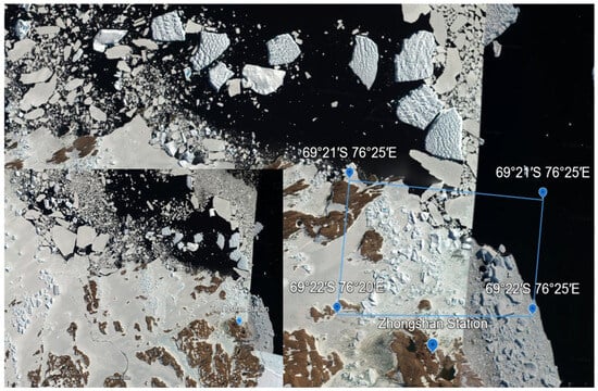
Figure 1. Location map of the study area.

The main contributions of this study are as follows.

• This research employs the ICI-YOLOv8 model to segment ice cracks in the imagery of the sea ice transport routes beyond Zhongshan Station in Antarctica. Ablation tests are conducted on a self-curated dataset with varying-scale models to substantiate the reliability and generalizability of the enhanced approach, thereby facilitating further analysis of the distribution and characteristics of ice cracks.
• The backbone of the model is redesigned with MobileNetV3 [33], providing a more lightweight structure while enhancing the ability to capture and emphasize critical features of ice cracks. In addition, the Wise-IoU [34] loss function is employed to replace the conventional bounding-box loss, and the SegNext_Attention [35] module is incorporated at appropriate positions within the network. These improvements collectively enhance the model’s capability in detecting and segmenting the complex characteristics of ice cracks with higher accuracy.
• A Monte Carlo simulation-based probabilistic model is proposed to quantitatively analyze ice crack distribution.

2. Methodologies

The main objective of this study is to enhance the YOLOv8-seg model by improving its backbone network, attention mechanism, and loss function. The architecture of the improved model is illustrated in Figure 2. Specifically, the original backbone is replaced with a lightweight MobileNetV3 [33] to mitigate the computational slowdown introduced by the convolutional attention framework SegNext_Attention [35]. The SegNext_Attention module is further incorporated at the junction between the backbone and neck networks, enabling multiscale information interaction and effectively addressing the challenge of large-scale differentiation in semantic segmentation targets. Moreover, Wise-IoU [34] is adopted to replace the conventional CIoU [36], thereby reducing harmful gradients and enhancing the overall detection accuracy. Finally, the density and fractal dimension of ice cracks are analyzed through Monte Carlo simulations under their corresponding probability density functions.

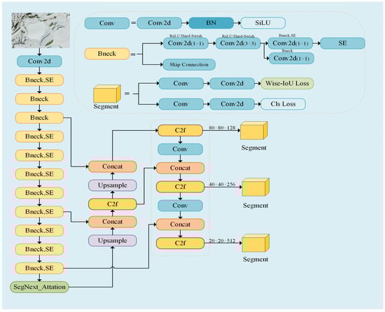
Figure 2. Structure of ICI-YOLOv8.

2.1. YOLOv8-Seg Algorithm Overview

In this paper, we choose YOLOv8-seg [37] as the baseline model, which is an instance segmentation submodel of the YOLOv8 generalized architecture that enables switching between the tasks of image classification, object detection, instance segmentation, and pose estimation by replacing modules. The YOLOv8 architecture belongs to the YOLO (You Only Look Once) [38] family of object detection models, which use a single neural network to predict the bounding boxes of objects in an image and their labels. The YOLOv8-seg model consists of three key components: the backbone network, the neck network, and the prediction head. The backbone network is the core component of the model and is responsible for extracting features from the input RGB color image. The neck network is located between the backbone network and the prediction head and is primarily responsible for aggregating and processing the features extracted from the backbone network. The neck and head networks are then used to predict the bounding boxes and labels of the objects in the feature map.

YOLOv8-seg uses a backbone similar to that of YOLOv5 [23], but with modifications in the CSPLayer to include the C3 module and the CSPLayer from YOLOv7 [39]. The learned Efficient Layer Aggregation Network (ELAN) is combined, now called the C2f module, replacing YOLOv5’s C3 module with a more gradient-rich C2f module, with the number of channels tuned for different model scales. The C2f module consists of a dual-convolutional split partial bottleneck that combines advanced functionality with contextual information to improve detection accuracy. At the end of the backbone network, the widely used SPPF [23] module is retained, which performs three maximum pooling operations of size 5 × 5 in sequence and concatenates each layer. As a result, YOLOv8 can obtain rich gradient flow information while remaining lightweight.

For the neck component, YOLOv8-seg uses PAN-FPN [40] for multilevel feature fusion, which fully utilizes the feature information at different scales so that ice cracks at various scales can be effectively identified.

The prediction head is the top-level component of the YOLOv8 model, which identifies and localizes object classes in the image. The segmentation head consists of three branches: bounding-box regression, classification, and mask segmentation. Meanwhile, YOLOv8-seg employs an anchorless model to generate proposal regions and accelerate detection and segmentation. For bounding-box loss, the CIoU [36] and the DFL [41] loss functions are used for training. For classification loss, the classification branch generates a tensor of size N × H × W (number of categories, height, and width of the feature map), which is trained using binary cross-entropy loss. These loss functions enhance object detection performance, particularly when dealing with smaller objects.

YOLOv8-seg utilizes the YOLACT [42] mask segmentation head, where the final mask is obtained by a single matrix multiplication and sigmoid activation function, as shown in Equation (1):

$$M=\sigma (P{C}^T)$$

(1)

where P is the 3D tensor of H_proto × W_proto × 32 representing the prototype mask, and C is the N × 32 tensor of the mask coefficients of N instances (N is the total number of positions of P3, P4, and P5 in the feature maps at different levels). The prototype network ProtoNet generates the prototype masks with the P3 feature map. Simultaneously, the segmentation branches are trained using a binary cross-entropy loss function to optimize the segmentation results.

2.2. Related Work of ICI-YOLOv8

ICI-YOLOv8 employs the lightweight backbone MobileNetV3-Small [33], since we found that the Large version does not provide additional accuracy improvement compared with the Small one. The use of depthwise separable convolutions significantly reduces the number of parameters and computational cost. By introducing the SE [43] (Squeeze and Excitation) module and H-swish activation function, computational efficiency is ensured, and high accuracy is preserved. The SE module enables MobileNetV3 to capture and emphasize essential ice crack features more efficiently and suppress unimportant features, thus improving the model’s detection capability. H-swish is used in the bottleneck block (Bneck) instead of some traditional ReLU activation functions to implement a mixed-use strategy. H-swish provides richer nonlinear expressiveness, which helps capture more complex features and improve model performance. Additionally, it provides smoother activation in the region where the input value is close to 0, which is more computationally efficient. Compared with ReLU, H-swish reduces instances where input values are truncated to zero by the activation function, which enhances the model’s training. Equations (2) and (3) show the definition of H-swish:

$$H-swish(x)=x\cdot {\displaystyle \frac{ReLU6(x+3)}{6}}$$

(2)

$$ReLU6(x)=\min (\max (0,x),6)$$

(3)

where x is the input value, and ReLU6(x) is the ReLU function, which restricts the input value between 0 and 6. The output values are normalized by division by 6 to ensure that the output range of the H-swish function is similar to the distribution of the original input values. The pseudocode for this structure is presented in Algorithm 1:

Algorithm 1: MobileNetV3 Backbone in ICI-YOLOv8

Initialize:     backbone = MobileNetV3 with depthwise convolutions, SE modules, H-swish activation Input: x = input image tensor (e.g., 3 × 640 × 640) Output: features = extracted feature maps features = backbone(x) # Apply depthwise conv, SE, H-swish Return features

SegNext_Attention [35] is a simple convolutional network architecture designed for semantic segmentation, consisting of an encoder, an attention mechanism, a decoder, and a loss function. It uses a robust backbone network as an encoder that allows for multiscale information interaction, and the module is able to learn the feature representation of the ice crack region and highlight these features during the decoding process to improve the accuracy of the model’s segmentation of ice cracks. This module processes all feature maps output from the backbone, including high-, medium-, and low-resolution features, while keeping the input/output resolutions unchanged. It first applies attention enhancement to multi-scale features, which are then fed into the Concat and Upsample operations of the PAN-FPN pathway.

The structure of the encoder (MSCAN) is shown in Figure 3a. It consists of four stages with gradually decreasing spatial resolution; each stage contains a downsampling block and an MSCA module. The downsampling block is implemented by a 3 × 3 convolution with a stride size of 2, followed by batch normalization. Batch normalization [44] improves segmentation performance, and integrating SegNext_Attention between the backbone and the neck increases the computational overhead of the system. However, it enhances the segmentation accuracy for ice cracks.

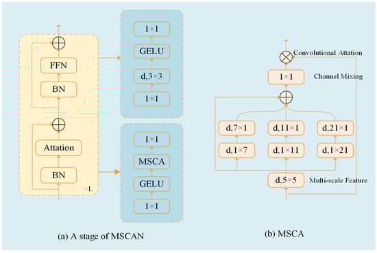
Figure 3. Structure of MSCA and MSCAN. Where L represents the number of times the Attention + FFN structure is repeated, and d, k1 × k2 denotes the deep convolution using a kernel size of k1 × k2, which is utilised to extract multiscale features, which are then used as attention weights to reweigh the inputs to the MSCA.

Figure 3b shows the structure of the Multi-Scale Convolutional Attention (MSCA) module, which consists of three parts: deep depthwise convolution for aggregating local information, multi-branch depthwise strip convolution for capturing multiscale context, and 1 × 1 convolution for modeling the relationship between different channels. This is represented by the following Equations (4) and (5):

$$Att=Con{v}_{1\times 1}\left({\displaystyle \sum _{i=0}^{3}S}cal{e}_i\left(DW-Conv(F)\right)\right)$$

(4)

$$Out=Att\otimes F$$

(5)

where F is the input feature map, and DW-Conv(F) denotes the depthwise convolution operation on F. Scale_i denotes the output of the i-th multiscale convolution branch, where the output features of all branches are weighted and summed (here, there are four branches) and recombined by 1 × 1 convolution to obtain the attention weight Att. ⊗ denotes the element-wise multiplication of the input feature map with the attentional weights to generate a weighted feature map. Pseudocode is shown in Algorithm 2:

Algorithm 2: SegNext_Attention Module in ICI-YOLOv8

Initialize: attention = SegNext_Attention incorporating MSCA with multi-scale convolutional attention Input: features = input feature maps from backbone Output: features = processed feature maps with attention features = attention(features) # Performs downsampling and applies MSCA with depthwise and multi-branch convolutions Return features

The implementation of YOLOv8 target segmentation requires the detection task results to contribute, so the model’s total loss function L is composed of the bounding-box loss together with the mask loss, as shown in Equation (6):

$$L=L_{\mathrm{box}}+L_{\mathrm{mask}}$$

(6)

where L is the average binary cross-entropy loss, L_box is the bounding-box loss, and L_mask is the mask loss.

Initially, YOLOv8-seg uses Complete Intersection over Union (CIoU) [36] as the default for calculating the bounding-box loss. CIoU introduces the aspect ratio of the predicted bounding-box and ground-truth bounding-box based on the Distance Intersection over Union (DIoU), making the loss function more focused on the shape of the bounding-box, as in Equations (7)–(9):

$$L_{CIOU}=L_{IOU}+{\displaystyle \frac{{(x-x_{gt})}^2+{(y-y_{gt})}^2}{w_g^2+h_g^2}}+\alpha v$$

(7)

$$\alpha ={\displaystyle \frac{v}{L_{IOU}+v}}$$

(8)

$$v={\displaystyle \frac{4}{{\pi }^2}}{\left(\arctan {\displaystyle \frac{w_{gt}}{h_{gt}}}-\arctan {\displaystyle \frac{w}{h}}\right)}^2$$

(9)

where L_IoU is the Intersection over Union (IoU) [45] loss, x and y are the coordinates of the centroid of the predicted box, x_gt, y_gt are the coordinates of the centroid of the ground-truth box, W_g and H_g are the width and height of the smallest rectangular box formed by the predicted and ground-truth boxes, α is a hyperparameter, v measures the consistency of the width and height ratios, and w and h are the width and height of the predicted box, respectively.

However, the computation of CIoU loss is relatively complex, resulting in significant computational overhead during training, and it only reflects the relative difference between aspect ratios, which cannot accurately localize. The prediction of bounding boxes directly affects the quality of the instance masks in the segmentation task. Therefore, Wise-IoU [34] is proposed as a dynamic nonmonotonic focusing mechanism that replaces bounding-box loss with phase anisotropy instead of IoU to evaluate the quality of anchor boxes. It uses a gradient gain assignment strategy to reduce the competitiveness of high-quality anchor boxes and mitigate the harmful gradients generated by low-quality anchor boxes by dynamically adjusting the weights of each predicted region, allowing the model to focus more on regions of ice cracks that are difficult to segment correctly during training. Its calculation is shown in Equations (10) and (11):

$$L_{WIOU}=L_{IOU}\cdot \left({\displaystyle \frac{{(x-x_{gt})}^2+{(y-y_{gt})}^2}{w_g^2+h_g^2}}\right)\cdot \gamma$$

(10)

$$\gamma ={\displaystyle \frac{\beta }{\delta \alpha \beta -\delta }}$$

(11)

where δ and α are hyperparameters (in training, δ is set to 3 and α is set to 2), γ is the gradient gain used to adjust the loss weights, and β is the outlier degree, with γ = 1 when β = δ.

2.3. Numerical Analysis of Ice Crack Density and Fractal Dimension Based on Probability Distribution

The binarized mask image derived from UAV aerial photography for ice crack processing defines the ice crack density (ρ) as the ratio of the number of crack pixels to the total number of pixels. The box-counting method [46,47] is used to calculate the fractal dimension (D_f) to characterize the spatial complexity of the cracks. The specific steps include selecting a series of boxes with different sizes (r) based on the image pixels, identifying ice cracks in masked images, calculating the minimum number of boxes (N) required to cover the cracks for each box size, plotting double-logarithmic graphs where the horizontal axis is log(r) and the vertical axis is log(N), and obtaining the fractal dimension by calculating the slope of the best-fit line.

Since the probability density method can be used to characterize the distribution of random variables in ice crack analysis, the gamma distribution is suitable for characterizing the sparsity of crack density due to its right skewness. Monte Carlo simulation is widely used in uncertainty analysis to verify the statistical properties of the model through a large number of random samples, and we verify the fit of the probability density of ice crack distribution through Monte Carlo simulation.

By analyzing the distribution of ice cracks in the sample region, we assume that ρ follows a gamma distribution (ρ ~ Gamma (k, θ)), and since D_f ranges from 1 to 2, D_f is distributed using a truncated normal distribution, which enables quantification of the distribution of ice cracks via a probability density function. These are given in Equations (12) and (13):

$$f(\rho ;k,\theta )={\displaystyle \frac{{\rho }^{k-1}{e}^{-\rho /\theta }}{{\theta }^k\mathrm{\Gamma }(k)}}$$

(12)

$$f(D_f;\mu ,\sigma ,a,b)={\displaystyle \frac{\varphi \left(\frac{D_f-\mu }{\sigma }\right)}{\sigma \left[\mathrm{\Phi }\left(\frac{b-\mu }{\sigma }\right)-\mathrm{\Phi }\left(\frac{a-\mu }{\sigma }\right)\right]}},\hspace{0.33em}\hspace{0.33em}\hspace{0.33em}1\le D_f\le 2$$

(13)

where D_f is the random variable; µ is the mean, σ is the standard deviation, ϕ is the probability density function, Φ is the cumulative distribution function, and a and b are truncation points (a = 1, b = 2). For brevity, the pseudocode for the probability distribution is omitted in Algorithm 3:

Algorithm 3: Probability Distribution of Ice Crack Density and Fractal Dimension

Initialize:     ρ, r_values = box sizes # Calculate fractal dimension for r in r_values:     N_r = min boxes to cover ice cracks     plot log(r) vs. −log(N_r)     Df = slope of best-fit line # Define distributions     ρ_dist = Gamma(ρ)     Df _dist = TruncatedNormal(Df, a = 1, b = 2)     joint_pdf = ρ_dist × Df _dist Return ρ_dist, Df _dist, joint_pdf

Monte Carlo simulation, which has been widely validated in remote sensing image processing and geophysical studies for the analysis of complex spatial data, is a numerical computation method based on random number generation and statistical analysis that estimates the probabilistic properties of complex systems through simulation experiments. We use Monte Carlo simulations (100,000 iterations) to generate simulated data for ρ and D_f in order to validate the plausibility of the probability density model and to analyze the distributional characteristics of the ice crack spatial distribution. Through the Kernel Density Estimation (KDE) method, we further optimize the distributional fitting of these simulated data to more accurately reflect the actual distribution of ice crack densities and fractal dimension. Additionally, we incorporate spatial autocorrelation analysis, specifically Moran’s I index and its corresponding p-value, to assess the spatial clustering of regions with high density and high fractal dimension. This analysis helps identify regions that are highly spatially correlated and may be more sensitive to environmental changes. In this paper, Q is defined as the product of ρ and D_f (Q = ρ × D_f) to simulate distributions reflecting the spatial correlation of crack density and complexity, providing numerical support for identifying high-risk regions and optimizing transport routes. For brevity, the pseudocode for the validation of the Monte Carlo simulation is presented in Algorithm 4:

Algorithm 4: Monte Carlo Simulation for Ice Crack Distribution Validation

Initialize:     num_simulations = 100,000, ρ_samples, Df_samples, Q_samples = empty lists # Generate data for i from 1 to num_simulations:     ρ = sample from Gamma     Df = sample from TruncatedNormal (a = 1, b = 2)     Q = ρ × Df     append ρ, Df, Q to ρ_samples, Df_samples, Q_samples # Analyze     ρ_kde = fit KDE to ρ_samples     Df_kde = fit KDE to Df_samples     Q_kde = fit KDE to Q_samples     morans_I = compute Moran’s I # Validate     validate =ρ_kde matches Gamma and Df_kde residuals ≈ Normal     high_risk = regions where Q_kde exceeds threshold Return validate, ρ_kde, Df_kde, Q_kde, morans_I, high_risk

We also explore the potential correlation between the distribution of ice cracks and global sea ice trends, as well as climate models. Based on the ice-albedo feedback theory proposed by Perovich [48], we hypothesize that there is a correlation between ρ (crack density) and changes in albedo, using it as a proxy variable for albedo changes. Through Monte Carlo simulations, we verified the probability distributions of ice crack density (ρ) and fractal dimension (D_f). These simulation results can be compared with sea ice extent data from the National Snow and Ice Data Center (NSIDC) and model predictions from the Coupled Model Intercomparison Project Phase 6 (CMIP6) [49], for example, the overlap between areas with high ρ and areas of sea ice reduction, to analyze the contribution of ice cracks to the reduction of sea ice. Furthermore, the MODIS MCD43A3 data can be used to estimate the albedo changes associated with ρ, indirectly verifying the impact of ice cracks on sea ice melting, further enhancing the relevance of this study to climate change research.

3. Experiment

3.1. Experimental Setup

The model training environment was a Windows 11 operating system, a 12th Gen Intel^® Core^TM i9-12900 K at 3.20 GHz, 64 GB RAM, and an NVIDIA GeForce RTX 3060 TI running the PyTorch 2.1.0 deep learning framework with Python 3.11.

The model training parameters are set as follows: the training epoch is 400, the batch size is 4, the number of processing iterations is 4, and the input image size is 640 × 640. The model is optimized using the AdamW optimizer, with an initial learning rate of 0.002. Training employs an early stopping mechanism, which terminates automatically when the validation loss stabilizes, ensuring model convergence. A weight decay strategy with a value of 5 × 10⁻⁴ is used to prevent overfitting. Other parameters are consistent with those used in the original YOLOv8-seg. The pretrained YOLOv8-seg-n weights, representing the smallest YOLOv8-seg model size, are used to reduce training costs. All other configurations remain consistent with the default settings of the original YOLOv8-seg model.

3.2. Introduction to the Dataset

The dataset used in this study is sourced from the 38th Chinese Antarctic Scientific Expedition, comprising orthophotos of ice cracks along the sea ice transportation route near Zhongshan Station, captured via unmanned aerial vehicle (UAV) aerial photography. The images, acquired using a DJI Matrice 350 RTK drone with a DJI Zenmuse P1 camera (35 mm focal length) at a flight altitude of 236.3 ± 0.2 m, have a resolution of 8192 × 5460 pixels. To prevent overfitting during training and enhance the generalization capability of the model, data augmentation techniques were applied to the sea ice crack samples. That is, the following augmentation operations were performed on each original image: random rotation (with an angle range of −30° to 30°), random cropping (the cropped image was uniformly resized to 224 × 224 pixels, and the cropped area accounted for 0.8–1.0 of the original image area) and random horizontal flipping. The cracks in the images were then annotated using labelme [50] to generate the corresponding JSON label files. To ensure annotation consistency, all labeling was performed by the same researcher and subsequently subjected to multiple manual reviews to minimize potential errors. The annotations cover various crack morphologies, including long linear cracks, short curved cracks, and partially branched cracks. Owing to the constraints of the acquisition area and the natural distribution characteristics, the number of different crack types is imbalanced. A total of 266 ice crack images were obtained, split into training and validation sets at an 80:20 ratio.

In addition, the remote sensing images of the target observation area have a relatively small spatial extent with limited coverage, and large-scale annotated datasets are lacking. Considering the trade-off between accuracy and cost, UAV-borne data are the most suitable for addressing the research objectives of this study. The dataset also includes generic water body data acquired by Sentinel-2 (available at https://www.kaggle.com). Both water bodies and sea ice cracks exhibit linear or narrow-strip patterns with clear but irregular boundaries, and thus the water body dataset can serve as a proxy task to partially validate the segmentation performance of the model on such targets.

3.3. Assessment of Indicators

In the experiments, pixel mean accuracy (mPA), mean Intersection over Union (mIoU), and mean Dice coefficient (mDice) were selected as evaluation metrics for semantic segmentation.

The pixel mean accuracy (mPA) is calculated in Equation (14):

$$\begin{gathered} P{A}_i={\displaystyle \frac{T{P}_i}{T{P}_i+F{N}_i}} \\ mPA={\displaystyle \frac{1}{C}}{\displaystyle \sum _{i=1}^{C}P}{A}_i \end{gathered}$$

(14)

where C is the total number of categories, PA_i is the pixel accuracy for category i, TP_i is the number of pixels in category i that were correctly predicted to be in that category, and FN_i is the number of pixels in category i that were incorrectly predicted to be in other categories.

The mean Intersection over Union (mIoU) and mean Dice (mDice) coefficients are calculated as in Equations (15) and (16):

$$mIoU={\displaystyle \frac{1}{C}}{\displaystyle \sum _{i=1}^{C}I}o{U}_i$$

(15)

$$\begin{gathered} Dic{e}_i={\displaystyle \frac{2\times T{P}_i}{2\times T{P}_i+F{P}_i+F{N}_i}} \\ mDice={\displaystyle \frac{1}{C}}{\displaystyle \sum _{i=1}^{C}D}ic{e}_i \end{gathered}$$

(16)

IoU_i is the intersection-over-union ratio of the i-th category, TP_i is the true positive instance of the i-th category, FP_i is the false positive instance of the i-th category, i.e., the number of pixels that were incorrectly predicted to be in that category, and FN_i is the false negative instance of the i-th category, i.e., the number of pixels that were incorrectly predicted to be in other categories.

Other segmentation models were evaluated using precision, recall, mean Average Precision (mAP), and Frames Per Second (FPS) as metrics.

Precision is the proportion of correctly predicted positive samples among all predicted positive samples, while recall is the proportion of correctly predicted positive samples among all actual positive samples. Precision and recall are calculated as in Equations (17) and (18):

$$P={\displaystyle \frac{TP}{TP+FP}}$$

(17)

$$R={\displaystyle \frac{TP}{TP+FN}}$$

(18)

Here, TP represents true positives (correctly predicted positive samples), FP represents false positives (samples incorrectly predicted as positive), and FN represents false negatives (positive samples incorrectly predicted as negative). A sample with an IoU greater than or equal to the confidence threshold is classified as positive, while one with an IoU below the threshold is classified as negative.

The average precision (AP) is calculated by Equation (19):

$$AP={\displaystyle {\int }_0^{1}P}(t)dt$$

(19)

Here, AP is a measure of the area under the Precision-Recall (P-R) curve, t is a variable for Recall, representing continuous Recall values ranging from 0 to 1, and P(t) denotes the corresponding Precision when the Recall is t.

For multiple classes of detected targets, the mean value of accuracy for each class is expressed in Equation (20):

$$mAP={\displaystyle \frac{{\displaystyle \sum _{n=1}^{N}A}{P}_n}{N}}$$

(20)

where N is the total number of categories, AP_n is the Average Precision for the n-th category, and the category in this study is ice cracks. The mAP@0.5 is used as the primary accuracy evaluation metric.

FPS, representing the number of frames processed per second by the network, is calculated as shown in Equation (21):

$$FPS={\displaystyle \frac{1}{preprocess+inference+NMS}}$$

(21)

Preprocess, inference, and NMS are the times used for model preprocessing, inference, and non-maximal suppression, respectively, and their sum represents the time required to process an image.

4. Results

4.1. Comparison with Other Models

To evaluate the detection performance of the ICI-YOLOv8 model, we tested it on the publicly available Sentinel-2 remote sensing water body dataset and an ice crack dataset from sea ice transport routes near Zhongshan Station, Antarctica. Initially, we compared the validation subset of these datasets using typical semantic segmentation models, U-Net and DeepLabV3+, with pixel mean accuracy (mPA), mean Intersection over Union (mIoU), and mean Dice coefficient (mDice) as evaluation metrics. The results are presented in Table 2 and Table 3.

Table 2. Comparison of results from two models on remotely sensed water body datasets.

Model	mPA	mIoU	mDice
U-net [12]	0.546	0.410	0.544
DeepLabV3+ [13]	0.522	0.387	0.520

Note: Bold type indicates the best-performing, and the same applies to the subsequent tables.

Table 3. Comparison of results from two models on the ice cracks dataset.

Model	mPA	mIoU	mDice
U-net	0.505	0.497	0.506
DeepLabV3+	0.503	0.496	0.503

Through the analysis of these tables, we observed that U-Net outperforms DeepLabV3+ in recognition performance. However, both semantic segmentation models show suboptimal performance on these datasets, prompting the use of the ICI-YOLOv8 model to assess its recognition capabilities.

To further validate ICI-YOLOv8, we quantitatively compared its target segmentation performance against mainstream segmentation algorithms, including YOLOv5-seg, YOLOv7-seg, and YOLOv8-seg, using precision (P), mean Average Precision (mAP@0.5), and Frames Per Second (FPS) as metrics. These results, tested on the validation subset, are shown in Table 4.

Table 4. Comparison of results from different models on remotely sensed water body datasets.

Model	P (Precision)	mAP@0.5	FPS
YOLOv5-seg	0.777	0.511	175.44
YOLOv7-seg	0.769	0.507	120.48
YOLOv8-seg	0.898	0.634	196.07
ICI-YOLOv8	0.933	0.657	188.67

Based on the analysis of Table 4, the ICI-YOLOv8 model proves to be the most effective. All its metrics surpass those of other algorithms. Compared with the base model, its precision increases from 89.8% to 93.3%, and mAP@0.5 rises from 63.4% to 65.7%. It achieves improved accuracy while maintaining a frame rate comparable to the original model, without compromising speed. Using the Sentinel-2 water body dataset, we demonstrated that modifications to the original YOLOv8-seg model enhance its recognition performance, outperforming other models.

We also evaluated these algorithms using offshore data from the 38th Chinese Antarctic Scientific Expedition, collected near Zhongshan Station. The results are presented in Table 5.

Table 5. Comparison of results from different models on the ice cracks dataset.

Model	P (Precision)	R (Recall)	mAP@0.5	FPS
YOLOv5-seg [23]	0.556	0.709	0.637	36.76
YOLOv7-seg [51]	0.561	0.713	0.634	26.04
YOLOv8-seg [36]	0.601	0.631	0.625	47.16
ASF-YOLO [28]	0.607	0.651	0.654	4.67
ICI-YOLOv8	0.628	0.698	0.662	40.65

Analysis of the ice crack dataset from Zhongshan Station’s sea ice transport routes shows that ICI-YOLOv8 outperforms other algorithms across all metrics, achieving the best results. Compared with the base model, its precision increases from 60.1% to 62.8%, and mAP@0.5 rises from 62.5% to 66.2%. Although its FPS is lower than that of the original model, it remains superior to that of other models. This confirms the effectiveness and generalization ability of our modifications to the YOLOv8-seg model. While ASF-YOLO achieves remarkable improvements, its training and validation time is substantially longer than that of the other models, which limits its advantage in terms of computational efficiency. Although U-Net and DeepLabV3+ are established semantic segmentation algorithms with certain advantages, ICI-YOLOv8’s high precision and speed make it more suitable for these datasets. The accuracy of sea ice crack detection is lower than that of the water body data because the dataset contains considerable noise. In addition, uncertainties in the annotated boundaries arise from manual labeling as well as the influence of shadows and snow cover on certain cracks.

4.2. Ablation Studies

To evaluate the contribution of each module, we conducted ablation experiments using the YOLOv8-seg base model as the benchmark and the ice crack dataset. The quantitative metrics include precision, recall, mAP@0.5, and Frames Per Second (FPS). The results are detailed in Table 6.

Table 6. Ablation test results of ICI-YOLOv8 in this article.

Model	P (Precision)	R (Recall)	mAP@0.5	FPS
YOLOv8-seg	0.601	0.631	0.625	47.16
+ WIoU	0.650	0.597	0.639	39.52
+ MobileNetv3	0.529	0.643	0.583	75.75
+ SegNext_Attention	0.623	0.682	0.656	37.45
+ MobileNetv3+ WIoU	0.569	0.543	0.556	55.25
+ SegNext_Attention+ WIoU	0.570	0.698	0.647	31.15
+ MobileNetv3+ SegNext_Attention	0.600	0.698	0.654	44.44
+ All	0.628	0.698	0.662	40.65

Analysis of Table 6 shows that the base YOLOv8-seg model has a precision of 60.1%, a recall of 63.1%, an mAP@0.5 of 62.5%, and an FPS of 47.16. The ICI-YOLOv8 model improves precision from 60.1% to 62.8% and mAP@0.5 from 62.5% to 66.2%. Although its FPS decreases, the overall performance remains robust.

Introducing the Wise-IoU (WIoU) loss function alone slightly improves precision and mAP@0.5 but reduces FPS compared to the base model. This indicates that WIoU enhances detection performance at the cost of computational speed. Incorporating the MobileNetv3 backbone significantly increases FPS to 75.75, a 28.59% improvement, but reduces precision and mAP@0.5. Thus, MobileNetv3’s lightweight design enhances inference speed but compromises detection accuracy. The SegNext_Attention module alone improves recognition, with mAP@0.5 reaching 65.6%, but significantly reduces FPS. The combination of WIoU and MobileNetv3 performs poorly, suggesting a conflict in optimization goals. An attention module is necessary to balance these effects and improve recognition.

We observed a performance degradation when combining MobileNetV3 with Wise-IoU, which can be attributed to the feature compression strategy of MobileNetV3. Specifically, its use of channel pruning and depthwise separable convolutions substantially reduces computational cost but simultaneously weakens the representation of fine boundary details. Since the strength of Wise-IoU lies in precise bounding box optimization, its advantage cannot be fully exploited when the input features lack sufficient boundary information, leading to a decline in performance. For the combination of WIoU and SegNext_Attention, the precision is 57.0%, the mAP@0.5 is 64.7%, and the FPS is 31.15. This configuration improves mAP@0.5 by 2.3% compared to the base model. It enhances detection performance but reduces inference speed. The combination of MobileNetV3 and SegNext_Attention achieves an accuracy of 60.0% and an mAP@0.5 of 65.4%, showing a clear improvement. This configuration maintains relatively high FPS while preserving satisfactory detection performance. The reduction in FPS compared with the baseline is mainly attributed to the SegNext_Attention module, whereas the role of MobileNetV3 lies primarily in overall parameter compression and inference stability rather than completely offsetting the additional computational complexity introduced.

Combining all modules increases precision to 62.8% and mAP@0.5 to 66.2%, with improvements of 2.7% and 3.7%, respectively. Although the computational burden reduces FPS to 40.65, the speed remains comparable to that of the base model. This configuration performs best on the remote sensing water body dataset, showing strong generalization. The integration of WIoU and SegNext_Attention enhances detection in complex backgrounds, while MobileNetv3 improves lightweight properties and real-time performance without significantly compromising accuracy.

4.3. Visualisation of Test Results

In addition to quantitative comparisons of the ICI-YOLOv8 model using precision, recall, and mAP@0.5, Figure 4 presents the detection results for sea ice cracks, and Figure 5 shows the results for remote sensing water bodies. To clearly compare recognition performance, precision values are included in the result visualizations for algorithms of the same type.

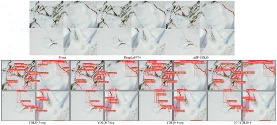
Figure 4. Identification results of ice cracks (the dark red part is the identified result).

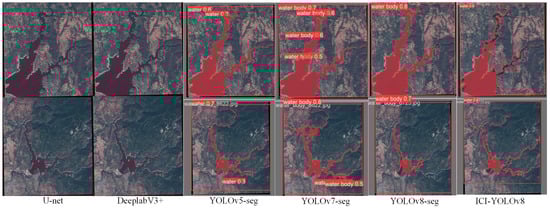
Figure 5. Identification results of remotely sensed water bodies.

5. Correlation Analysis of Ice Cracks

5.1. Distribution of Ice Cracks

Figure 6 shows the modelling map of some sample areas. The camera model, flight altitude, and focal length carried by the unmanned aerial vehicle (UAV) allow us to determine the ground sampling distance (GSD) of the images, which is approximately 29.5 mm/pixel, enabling the determination of the actual size of the cracks. The analysis of ice cracks in the sample area of the sea ice transport route around Zhongshan Station includes elements such as the size, area, number, and density of ice cracks.

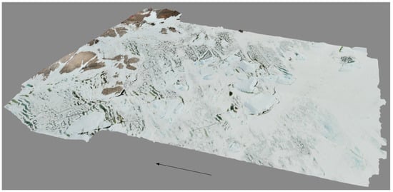
Figure 6. Partial sample area of ice cracks (arrow direction from sea ice to Zhongshan Station).

Through ICI-YOLOv8’s detection of the orthophotos, we determined that there were approximately 16,949 ice cracks in the sample area, with varying sizes and shapes, and that the majority of these ice cracks in the orthophotos were less than 2 m in length, with the longest having exceeding 20 m; widths of less than 2 m also accounted for the majority of the cracks. Figure 7 shows the statistics of the area, length, and width of the ice cracks in some sample areas. The average length of the ice cracks in this area is 0.36 m, and the average width is 0.194 m. Through analysis, the ice cracks in the region have the following characteristics: the shorter-length ice cracks cross each other and have wider widths, are accompanied by broken sea ice and seawater, and are distributed in a curved line, while those longer-length ice cracks do not cross each other, are larger, and are distributed in a straight line, as shown in Figure 8, which is the identification result of the ice cracks in the sample region.

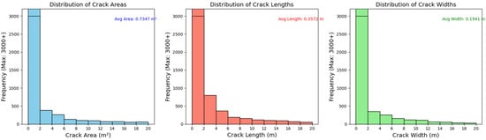
Figure 7. Results of the identification of ice cracks.

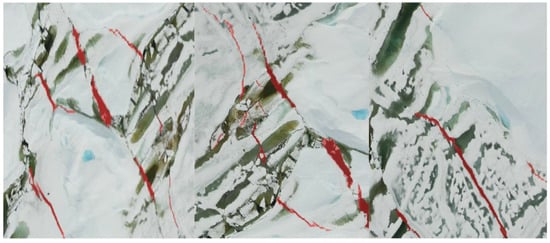
Figure 8. Distribution of ice cracks in orthophotos.

Figure 9 shows the distribution of some ice cracks in the sample area on the transport route around Zhongshan Station, from which we can observe different densities of ice crack distribution. We infer that the areas with higher ice crack density may be the weak points in the ice, subject to drastic temperature variations, or affected by water currents and pressure buildup; areas with lower crack density may be more stable or experience fewer external influences compared to the former. Because the density of ice cracks affects the stability of sea ice and the safety of transport routes over sea ice, we constructed the complete region in Figure 10 in 2D and divided this into 20 × 36 grid areas, calculating that each grid represents an actual 40 × 40 m area, as in Figure 11. We assigned scores to ice cracks based on the ice crack coverage area per grid unit. The higher the score, the greater the ice crack coverage area, the higher the ice crack density, and the more dangerous the area. By analyzing the ice crack coverage area in Figure 10, we obtained the distribution of ice crack scores in Figure 11.

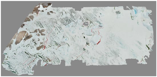
Figure 9. Distribution of selected ice cracks in the sample area.

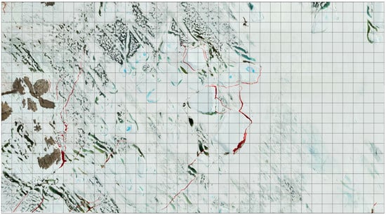
Figure 10. Map of ice-crevassing divisions in the sample area.

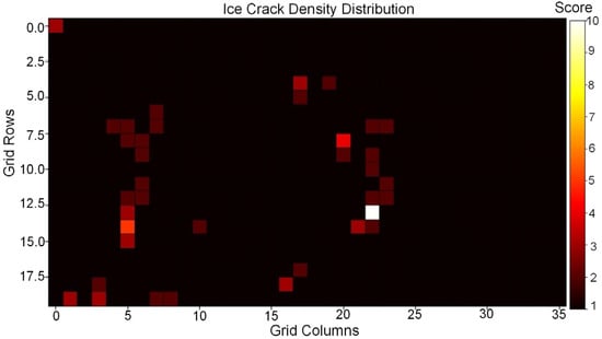
Figure 11. Distribution of ice crack scores in the sample area.

By analyzing Figure 11, we found that the ice cracks are centrally distributed, concentrated in the middle and lower parts of the area; darker colored areas, such as crimson, indicate low ice crack coverage, and these areas are relatively safe, while brighter colored areas indicate higher ice crack coverage, making them more dangerous, and the white colored areas in the figure are the most dangerous, requiring avoidance. For the distribution of ice cracks in the nearshore sea, we used the improved RRT* algorithm [52] by binarizing the region to automatically plan the safest route with the lowest cost (run repeatedly 30 times with different random seeds, and the average path cost was taken as the final result), as shown in Figure 12.

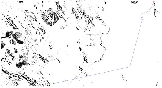
Figure 12. Schematic diagram of path planning in the sample area (red dots are start points, green dots are endpoints).

We assumed that the starting point is the docking position of the icebreaker, and the endpoint is near Zhongshan Station in China. The straight-line distance between the starting point and the endpoint is the shortest, but the route’s ice crack coverage area is too large, compromising safety. Through Figure 12, we found that the algorithm planned the route to avoid most areas with high ice crack coverage, corresponding well to the ice crack score map in Figure 11, perfectly avoiding dangerous areas, but it cannot completely avoid small sea ice cracks. Additionally, the planned route is relatively close to the sea ice area where seawater seeps out. To address this issue and consider time cost, transport efficiency, and safety, constructing a bridge over the sea ice cracks for transport is an effective method.

5.2. Stability Analysis of Ice Cracks

Ice cracks act as a conduit for heat exchange between the atmosphere and the ocean, and ice cracks expose the interior of the sea ice, allowing direct solar radiation to contact the ice and accelerate sea ice melting. Research [32] found that temperature has a direct effect on the expansion of ice cracks, and found that at lower temperatures (−25 °C), the global KR curve behavior is positive, i.e., the overall fracture resistance increases with ice crack expansion. KR is part of the stress intensity factor (K), which represents the state of stress within the material to resist crack expansion, and the higher the value of KR, the greater the resistance of the material to crack expansion. However, at higher temperatures (−15 °C), although the overall fracture resistance may increase with crack extension, the crack may exhibit localized negative KR behavior in certain localized regions or phases. This means that in these localized regions, the fracture resistance may transiently decrease, leading to faster crack extension and potentially triggering sudden sea ice destruction [32]. This localized negative KR behavior results from higher temperatures causing the mechanical properties of ice to exhibit more plastic characteristics, making stress concentration and localized weakening more likely to occur during crack extension.

When ice cracks form and expand, seawater may seep out through the cracks, and the accelerated rate of crack expansion further damages the structural integrity of the sea ice and provides a channel for seawater to seep out [32]. After seawater seeps out, the seawater in the cracks will absorb more solar radiation because the absorption rate of water is higher than the reflectivity of ice, and this absorption increases the heat flux of the sea ice, further accelerating sea ice melting.

Figure 13 shows a schematic diagram of the heat exchange modeling of sea ice, the atmosphere, and the ocean along the transport routes, as well as thermal imaging of sea ice, ice cracks, and snow, which was obtained from aerial photography by a DJI drone. In the Antarctic summer, solar radiation is a primary sources of heat absorption in sea ice and can directly irradiate the ice between the ice cracks, which have a lower albedo than snow-covered areas due to the lack of snow cover, allowing more solar radiation to be absorbed by the ice; whereas the high albedo of the snow causes most of the radiation being reflected [53]. In the thermal images, ice cracks and dark sea ice regions without snow cover are brighter colored, indicating that their temperatures are significantly higher than those of surrounding snow-covered areas. Antarctic sea ice has a higher thermal conductivity than air [48], and ice crack regions and exposed dark-colored sea ice regions conduct absorbed solar radiation downward more efficiently (intra-ice conduction); additionally, the lack of snow cover exposes these regions directly to the atmosphere, resulting in higher surface temperatures and enhanced sensible heat fluxes to the atmosphere, particularly at higher temperatures in summer. Thus, the combined effect of heat conduction and sensible heat processes results in significantly higher heat fluxes in these regions than in snow-covered areas.

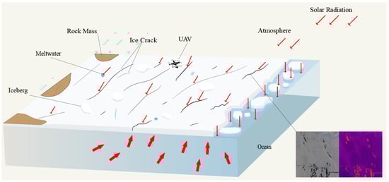
Figure 13. Schematic diagram of heat exchange between sea ice, atmosphere and ocean along transportation routes (arrows indicate the direction and quantity of heat transfer; the larger and more densely packed the arrows, the greater the amount of heat transferred), and the figure on the right is a thermal image of sea ice, ice cracks and snow.

The atmosphere transfers heat by conduction and convection to the sea ice and ice between ice cracks, particularly during the high atmospheric temperatures of the Antarctic summer. Changes in nearshore sea ice thickness at Zhongshan Station in Antarctica are primarily influenced by thermodynamic factors, including the effects of solar shortwave radiation and ocean heat flux [54], and ocean heat in eastern Prydz Bay is primarily transferred to the bottom of the sea ice through warm water currents driven by upwelling or oceanic currents, leading to bottom melting [55]. The Antarctic region is significantly affected by warm water currents, which markedly accelerate the rate of melting at the bottom of the sea ice in summer.

During China’s 38th Antarctic Scientific Expedition in the Antarctic summer, the temperature was relatively high, resulting in a decrease in fracture resistance. As shown in Figure 8, seawater seepage changes the color of the sea ice. Combined with the thermal imaging map in Figure 14, white snow-covered ice reflects most solar radiation [48], while ice cracks and darker regions are warmer and absorb more solar radiation, increasing heat exchange intensity and causing the ice to absorb more heat, thus increasing the ice’s heat flux. Furthermore, after seawater seeps through the cracks, the seawater becomes a pathway for heat transfer, and in the Antarctic low-temperature environment, seawater in the cracks not only has high thermal conductivity [56] but may also induce convection, becoming a more effective heat transfer pathway compared to the surrounding sea ice [56]. Additionally, the darker color and lower albedo of the cracked regions result in more solar radiation absorption, further increasing the heat flux through the ice. These factors collectively result in a significantly higher heat exchange intensity in the crack region than in the surrounding snow-covered areas, creating a positive feedback loop where increased heat flux continues to melt the sea ice. Therefore, these ice crack areas affect the planning and design of transport routes, and avoiding them increases time costs. However, small ice cracks have limited width and depth and do not penetrate deeply into the sea ice interior, so constructing bridges over small sea ice cracks on the transport routes is an effective method, as shown in Figure 14, enabling crossing small ice cracks to ensure safety and improve transport efficiency.

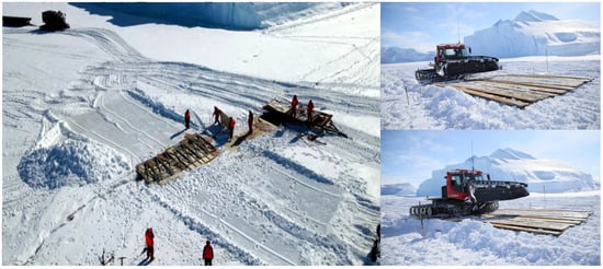
Figure 14. Schematic diagram of a bridge laid over a small ice crack.

Figure 15 presents the elevation map of the ice crack sample area shown in Figure 6. A qualitative analysis in conjunction with the crack detection results in Figure 10 and Figure 11 indicates that cracks are concentrated in regions with pronounced color variations in the elevation map, namely around icebergs within the sea ice or areas with significant height fluctuations, and they generally exhibit curved patterns corresponding to terrain depressions or faults. In contrast, cracks in other parts of the sea ice tend to display linear distributions. Icebergs in the sea ice and surrounding mountains are key factors influencing the distribution of ice cracks. During sea ice movement, internal icebergs move with it, exerting significant pressure on the ice and leading to stress concentration [57]. Simultaneously, surrounding mountains obstruct sea ice movement, causing internal ice to compress [58]. These stress-concentrated areas readily lead to the formation of new cracks in the ice or further extension of existing cracks [57]. Ice cracks are concentrated around icebergs or areas with significant height changes in sea ice, distributed in a curved pattern, and the movement of sea ice intensifies stress in these areas, readily leading to the formation of new cracks in the ice or further expansion of existing cracks.

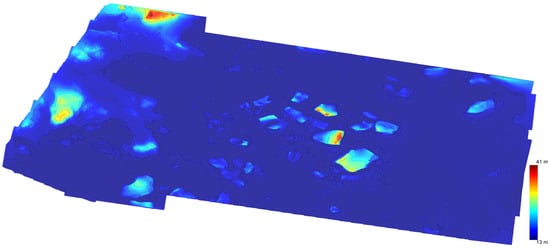
Figure 15. Elevation map of the sample area of the ice crack section (meters).

5.3. Correlation of the Fractal Dimension of Ice Cracks with the Density of Ice Cracks

In Figure 9 and Figure 10, the morphology of ice cracks is not in regular straight lines but extends, bifurcates, and intersects along several main cracks. Although different cracks vary in their geometric forms, there is a certain spatial similarity, i.e., self-similarity, in the distribution of ice cracks. The fractal dimension is used to describe the degree of irregularity of ice cracks in the context of fractal geometry, increasing as the irregularity of cracks increases. It is calculated by the box-counting method [46,47], involving converting the annotated JSON files into sea ice crack mask images, selecting a series of box sizes on a logarithmic scale, and covering the fractal cracks with these boxes. The number of boxes required at each scale is recorded, and a log–log plot of the number of boxes versus the inverse of the box size is then generated. The slope of the resulting line corresponds to the fractal dimension. Since UAV orthophotos provide only planar information, we selected crack distribution maps from different regions, as well as the sample area shown in Figure 11, to calculate their fractal dimensions. Figure 16 shows the results of analyzing the ice crack image in Figure 10 using the box-counting method, with a linear fit to the scatter plot of ln(r) versus −ln(N), where the slope is the fractal dimension of the image, D_f = 1.1211. Using the same method for ice crack images in other regions of the sample, the results show good agreement with power-law distributions (R² > 0.9), indicating significant fractal properties of the ice crack distribution.

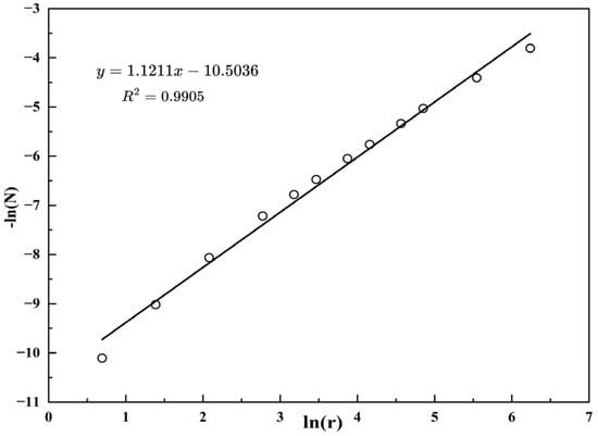
Figure 16. Number of grids N through which ice cracks pass in the sample area versus grid size r.

Lu [59] and Zheng [60] defined the ratio of the number of pixels occupied by sea ice cracks to the total number of pixels in the image as sea ice density in sea ice remote sensing image analysis. In this paper, we adopt this definition and define the ice crack density as ρ = n/N in the mask image with ice cracks, where n is the number of pixels with a value of 1 in the binary image and N is the total number of pixels in the image. We calculated ice crack density for the region used for fractal dimension calculation. Figure 17 shows that the fractal dimension D_f of ice cracks ranges from 1.121 to 1.681, and the density ρ of ice cracks ranges from 0.00293 to 0.03137 in the aerial images and the curve fitting results show a strong logarithmic relationship between D_f and ρ (R² > 0.96), indicating a significant positive correlation between ice crack density and fractal dimension. This can be interpreted as a positive feedback process from a fracture mechanics perspective. On one hand, higher crack density leads to more frequent interactions among cracks, facilitating branching and intersections that increase the complexity of the crack network. On the other hand, a more complex crack network enhances stress concentration and propagation pathways, thereby promoting the formation of new cracks and further increasing crack density [57]. When the ice crack density ρ approaches 1, the fractal dimension D_f approaches 1.99, indicating that the spatial dimension of ice cracks approaches two dimensions when the ice crack proportion in the image is nearly 1.

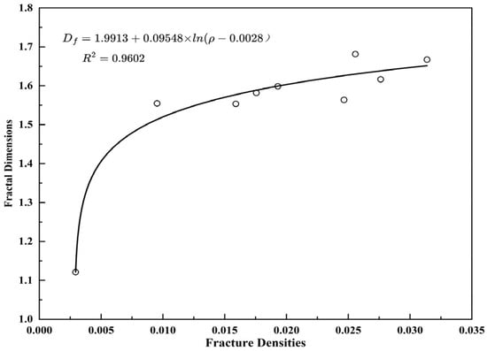
Figure 17. Ice crack density versus fractal dimension.

Weiss [61] demonstrated scale invariance in ice cracks and fragmentation patterns through extensive data, establishing a universal law of the ice crack fragmentation process, which describes ice cracks at different spatial scales using a unified fractal dimension D_f. The ice cracks density ρ in this paper is another key metric describing the number of ice cracks at different scales in the region, indicating a relationship between fractal dimension and crack density. This relationship exists because ice cracks are dynamically changing [62], and greater crack development results in increased irregularity of cracks at different scales (larger D_f) and larger crack coverage area (larger ρ). The coordinate points in Figure 17 include several maps of ice crack distribution in different regions (right-hand points) as well as the map of ice crack distribution after modeling the sample region in Figure 10 (starting point), and the fit (R² > 0.9) is high, illustrating this spatial correlation between the crack density ρ and the fractal dimension D_f through the crack morphology at different locations on the ice surface and at different scales.

To describe the statistical properties of ρ and D_f, we constructed a probability distribution model [63] for ρ and D_f in Figure 17 to investigate the probability that ice crack density ρ follows a gamma distribution with a probability density function:

$$p(\rho )={\displaystyle \frac{{\rho }^{5.71-1}{e}^{-\rho /0.00298}}{{(0.00298)}^{5.71}\mathrm{\Gamma }(5.71)}},\hspace{0.33em}\hspace{0.33em}\hspace{0.33em}\rho >0$$

(22)

That is, ρ ∼ Gamma (k = 5.71, θ = 0.00298), where k is a shape parameter controlling the skewness of the distribution, and θ is a scale parameter controlling the stretching of the distribution, and the mean and standard deviation were calculated to be consistent with the range in Figure 17.

The relationship between the fractal dimension and the ice crack density follows a conditional distribution, with a probability density function:

$$p(D_f|\rho )={\displaystyle \frac{1}{\sqrt{2\pi \cdot {0.06}^2}}}\exp \left(-{\displaystyle \frac{{(D_f-(0.09548\ln (\rho -0.0028)+1.9913))}^2}{2\cdot {0.06}^2}}\right)$$

(23)

The joint probability distribution is constructed through the marginal distribution of ρ and the conditional distribution of D_f, reflecting the logarithmic relationship and physical laws between the two, as in Equation (24):

$$p(\rho ,D_f)=p(D_f|\rho )p(\rho )$$

(24)

We verified the probability distributions by Monte Carlo simulation [63] to check consistency with the data characteristics of the fitted function in Figure 17. The marginal distribution of ρ and the conditional distribution of D_f were found to be reasonable. The scatter points in Figure 18a are distributed around the red curve, with small fluctuations, and their failure to cover the observed low values results from the larger scale of the coordinate points in Figure 10 compared to other coordinate points (e.g., Figure 8), resulting in a smaller ice crack proportion; the simulated distribution in Figure 18b agrees with the theoretical curve and is consistent with the gamma distribution assumption, exhibiting a right-skewed characteristic (high probability of low ρ, low probability of high ρ) aligned with the physical law (crack-sparse regions are more common); the residual distribution in Figure 18c is approximately normal with a mean of approximately 0, indicating that the simulated D_f has no systematic deviation around the fitted curve.

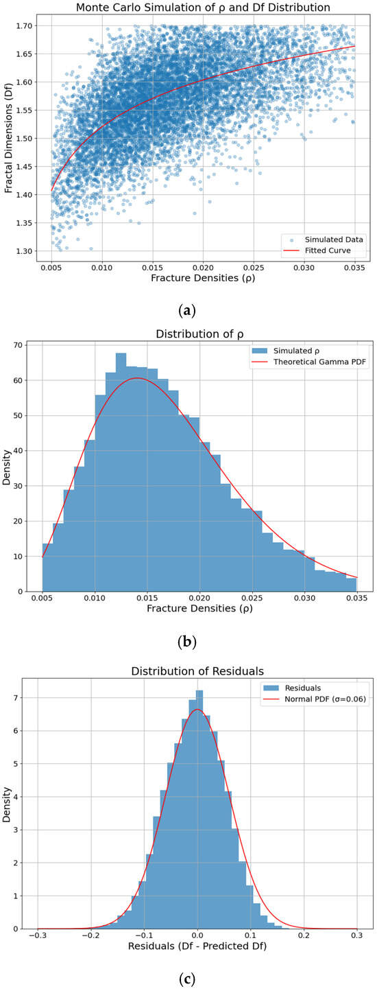
Figure 18. (a) Scatterplot of Monte Carlo simulations. (b) Distribution of ice crack density ρ (red curve is theoretical gamma distribution). (c) Residual distribution for D_f.

To study a larger sample region, such as Figure 10, we corrected the mathematical model constructed with ρ and D_f for this region. The region is divided into 20 × 36 grids, and we reflected the ice crack distribution probability in this region by analyzing each grid. Because many grids lack cracks, a threshold ρ ≥ 0.00005 was set to filter the grids, and to smooth noise and adjust the distribution, percentile filtering (50% quantile) with Gaussian smoothing (σ = 0.8) was applied, increasing the number of grids to 360 after filtering, with a mean ρ of 0.002931, effectively removing noise and resulting in a more concentrated ρ distribution, while preserving spatial heterogeneity.

The mean D_f after filtering (ρ ≥ 0.00005) is 1.558, lying within the range (1.121–1.681) in Figure 17, close to the upper limit, suggesting that the crack network has high complexity in the high-density region. To ensure the physical reasonableness of D_f in this region, scaling and standard deviation adjustments were applied, and the adjusted (filtered) mean D_f is 1.202, aligning with the physical interpretation of two-dimensional fractal dimensions and ensuring that the D_f distribution reflects the complexity variance of the cracks network while avoiding unphysical values. Table 7 presents the statistical results of the correlation, with a correlation coefficient between ρ and D_f of 0.713, slightly lower than R² in Figure 17, but indicating a significant correlation between ice crack density and complexity within the study area, influenced by external factors; Moran’s I, a measure of spatial autocorrelation, is positive, indicating spatial clustering, with higher values suggesting more pronounced spatial correlation, where similar values cluster together, indicating a concentrated distribution of high-risk areas.

Table 7. Relevant statistical results.

Norm	Average Value	Standard Deviation	Note
All grids ρ	0.002932	0.014895	-
Post-screening ρ	0.02104	0.034293	Mesh 105
Adjusted Percentile Screening ρ	0.002931	0.004691	Mesh 360
Df after screening	1.558	0.271	-
Adjusted Df	1.202	0.281	-
ρ and Df correlation coefficients	0.713	-	Support for logarithmic relationships
Q’s Moran’s I	0.723	p-value: 0.01	Significant spatial autocorrelation

Thus, the probability density function after fitting ρ and D_f is:

$$f(\rho )={\displaystyle \frac{{\rho }^{0.39-1}{e}^{-\rho /0.0075}}{{0.0075}^{0.39}\mathrm{\Gamma }(0.39)}},\hspace{0.33em}\hspace{0.33em}\hspace{0.33em}\rho >0$$

(25)

$$f(D_f)={\displaystyle \frac{\exp \left(-\frac{{(D_f-1.202)}^2}{2\cdot {0.281}^2}\right)}{0.281\sqrt{2\pi }\left[\mathrm{\Phi }\left(\frac{2-1.202}{0.281}\right)-\mathrm{\Phi }\left(\frac{1-1.202}{0.281}\right)\right]}},\hspace{0.33em}\hspace{0.33em}\hspace{0.33em}1\le D_f\le 2$$

(26)

where the simulated data for ρ were generated by kernel density estimation (KDE) and fitted to a gamma distribution, k = 0.39, θ = 0.0075, the gamma distribution is selected to model crack density ρ because it effectively captures the right-skewed distribution characteristics of crack density and accurately describes its asymmetric distribution pattern. As shown by the fitted curve, the gamma distribution effectively captures the right-skewed nature of the sample data. The simulated data for D_f were generated by kernel density estimation (KDE) and fitted to a truncated normal distribution; the range of D_f is constrained to the geometric interval [1, 2] based on physical practical implications, reflecting its concentrated distribution characteristics and limited interval range, μ = 1.202, σ = 0.281. The fitted curve closely matches the histogram of the simulated distribution, as shown in Figure 19. The probability density functions of ρ and D_f quantify the ice crack distribution probability and reflect the spatial distribution characteristics of ice cracks and their complexity from a macroscopic perspective.

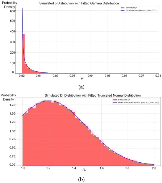
Figure 19. (a) Plot of the fitted distribution of ρ (blue solid line is the fitted gamma distribution, and the vertical coordinate indicates the probability density in 1/ρ). (b) Plot of the fitted distribution of D_f (solid blue line is the fitted truncated normal distribution, and the vertical coordinate indicates the probability density in 1/D_f).

In this paper, Q is defined as the product of ρ and D_f, used to synthesize the effects of ice crack density and complexity on sea ice stability. Monte Carlo simulations (100,000 iterations), combined with a kernel density estimate (KDE) of ρ and a truncated normal distribution of D_f, yielded a simulated distribution of Q. The mean value Q (0.004463) was calculated from the product of the mean of ρ and the mean of D_f plus the covariance of ρ and D_f. Figure 20 illustrates a heatmap of the spatial distribution of ρ, a heatmap of the spatial distribution of D_f, and a heatmap of the spatial distribution of Q. The high-value regions in these plots correspond to the ice crack distribution regions in Figure 11.

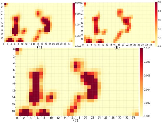
Figure 20. (a). Spatial distribution of ρ. (b). Spatial distribution of D_f. (c). Spatial distribution of Q.

The low-value region (ρ ≈ 0, yellow) in Figure 20a occupies most of the grid, reflecting the overall sparsity of crack density in the study area. The high-value regions of D_f (1.8–2.0) in Figure 20b highly overlap with the high-value regions of ρ, indicating that in crack-dense regions, the fractal structure of the cracks is more complex, potentially driven by local stress amplification and heat flux. This clustering is further confirmed by the spatial autocorrelation (Moran’s I = 0.723, p-value = 0.01) of the high-value regions in the spatial heatmap of Q in Figure 20c, which coincides with the high-value regions of ρ and D_f, suggesting that the sea ice may be at higher risk of rupture in these areas.

Figure 21 illustrates the simulated distribution of Q. The red histogram shows the simulated distribution of Q, generated using a Monte Carlo simulation. The blue solid line is the fitted lognormal distribution curve, which reflects the distributional characteristics of Q. The calculated mean Q is 0.004463 (black dashed line), obtained from the previous section. The 95% confidence interval of the simulated distribution is [0.000001, 0.009275] (the two ends of the interval are represented by two blue dashed lines), slightly lower than the theoretically calculated [0.001395, 0.009987], likely due to underestimation of tail probabilities caused by tail constraints and sample size limitations. The confidence intervals cover the calculated means despite small deviations (upper bound deviation of approximately 7%), indicating that the simulation results are generally consistent with the theoretical calculations. The Q distribution exhibits a right-skewed characteristic, with a peak around 0.002, reflecting the presence of high-risk regions.

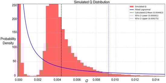
Figure 21. Modelled distribution of Q (vertical coordinate is the probability density in units of 1/Q, reflecting the density of the distribution of simulated values of Q).

Figure 22 illustrates the 3D surface of Q. The z-axis extent is aligned with the extent of the Q heatmap, verifying the spatial distribution of Q. The spatial distribution pattern is consistent with Moran’s I, showing significant spatial autocorrelation. The high-value region’s spatial distribution coincides with the distribution of ρ and D_f, consistent with the computational logic and positive correlation of Q. The positive correlation (0.713) of ρ and D_f is indirectly verified through the peak distribution of Q. Therefore, our proposed probability density function after fitting ρ and D_f is correct and reflects the spatial distribution characteristics of ice cracks, their complexity, and high-risk areas.

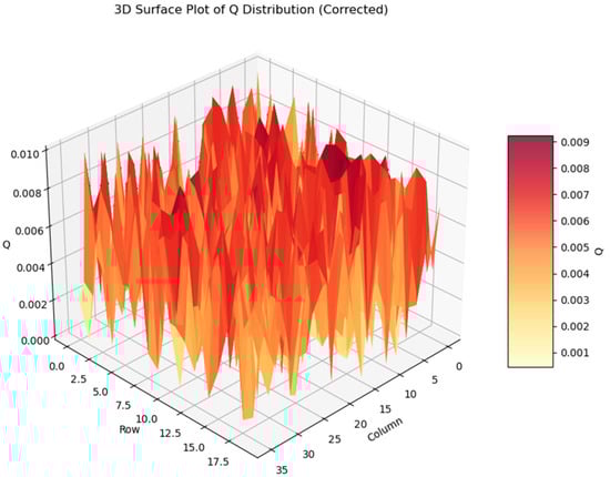
Figure 22. 3D surface view of Q.

6. Discussion

In this study, we explored the relationship between ice crack distribution and global sea ice trends and climate models, based on the ice-albedo feedback theory [48] and climate prediction models [64]. The ice-albedo feedback theory suggests [48] that ice crack density (ρ) increases the area of exposed seawater, reduces albedo, and increases heat absorption. We hypothesized that there is a correlation between ρ and albedo changes and used ρ from Monte Carlo simulations as a proxy for albedo changes. Equations (27) and (28) demonstrate that regions with high ρ exhibit greater albedo reduction and accelerated regional sea ice melting:

$${\alpha }_{\mathrm{eff}}=(1-\rho ){\alpha }_{\mathrm{ice}}+\rho {\alpha }_{\mathrm{water}}$$

(27)

$$\Delta Q_{\mathrm{rad}}=S\cdot (1-{\alpha }_{\mathrm{eff}})$$

(28)

where α_eff is the effective albedo, α_ice is the albedo of ice, α_water is the albedo of seawater, α_ice > α_water, and ρ is the ice crack density. ΔQ_rad represents the additional solar energy absorbed due to albedo reduction, and S is the solar radiation intensity.

In future research, these simulations can be compared with National Snow and Ice Data Center (NSIDC) sea ice extent data (2020–2023) to analyze the overlap between high-ρ regions and areas of sea ice reduction, suggesting a potential mechanism for the contribution of ice cracks to sea ice reduction. This approach aligns with sea ice change analysis methods and can validate the sensitivity of crack distribution to sea ice changes. Climate prediction models [64] predict an Antarctic sea ice decline by the mid-21st century, and Monte Carlo simulation results can be compared with these predictions to explain the overlap between ice crack distribution and areas of sea ice decline. D_f reflects the complexity of the ice crack network. The positive correlation between D_f and ρ was examined earlier, and Figure 21 shows the strong overlap in their heatmaps, indicating that high-D_f regions reduce albedo similarly to high-ρ regions.

Furthermore, using MODIS MCD43A3 data enables estimation of albedo changes. These data provide high-spatial-resolution albedo information and allow indirect analysis of the impact of ice cracks on sea ice melting. By analyzing the spatiotemporal albedo changes and comparing them with sea ice extent changes, we can further validate the relationship between Monte Carlo simulation results and the ice-albedo feedback theory.

Relevant studies and Antarctic Sea Ice data [49] indicate that Antarctic sea ice extent exhibited a clear downward trend from 2021 to 2023. In September 2021, the maximum Antarctic sea ice extent was approximately 18.5 million km², near the historical average. In September 2022, the maximum extent was 18.19 million km², still within the historical variability range. In September 2023, the maximum extent decreased to 16.96 million km², reaching a historical minimum. The sea ice area reduction reduces the mechanical strength of the sea ice, making it more susceptible to ice crack formation due to stress concentration. From a macroscopic perspective, this reflects the overall sea ice decline. From a microscopic perspective, there is a negative correlation between increased ice crack density and reduced sea ice extent. Therefore, based on Monte Carlo simulations, the mean ice crack density distribution significantly increases with area reduction, further confirming the negative correlation between sea ice area reduction and increased ice crack density, highlighting the impact of climate change on sea ice dynamics.

This study comprehensively analyzes the potential contribution of ice crack distribution to sea ice reduction by integrating ice-albedo feedback theory, NSIDC data, climate prediction models, and MODIS data. This integrated approach aligns with current climate change research theories and methods and provides a new research direction for understanding the complex mechanisms of sea ice change. Although this study did not fully validate these relationships, its theoretical framework and analytical approach provide a foundation for future research.

7. Conclusions and Outlook

In this study, we investigated the detection of ice cracks along the nearshore sea ice transport routes of Zhongshan Station, Antarctica, using unmanned aerial vehicle (UAV) aerial photography. The proposed ICI-YOLOv8 algorithm enhances both detection speed and accuracy for complex ice crack patterns compared to other algorithms, achieving a precision of 62.8% and a mean Average Precision (mAP@0.5) of 66.2%. Ablation studies confirmed the effectiveness and reliability of our approach. Through the identification and analysis of ice cracks, we drew the following conclusions:

(1)

The spatial distribution of ice cracks is distinct. Short ice cracks are primarily distributed in a curved and concentrated manner around areas where broken ice meets water bodies, as well as around the peripheries of icebergs or regions with significant sea ice height changes. In contrast, long ice cracks are primarily distributed in straight lines and rarely intersect.

(2)

Ice cracks affect sea ice heat flux and stability. In the Antarctic summer, high heat flux in ice crack and dark sea ice areas accelerates melting and reduces sea ice stability, indicating that ice cracks play a significant role in sea ice dynamics and climate change.

(3)

A probabilistic model developed for ice crack distribution effectively quantifies their distribution along the external transport routes of Zhongshan Station. This model, incorporating ice crack density (ρ) and fractal dimension (D_f), accurately fits the observed ice crack distribution. A Q-distribution based on Monte Carlo simulation quantifies the probability of ice crack distribution, highlighting high-risk areas. The morphological distribution of ice cracks across various locations and scales exhibits distinct fractal characteristics, with a significant logarithmic correlation between ρ and D_f in the aerial photography area.

This study focuses on summer sea ice along nearshore transport routes in Antarctica, which experiences higher temperatures compared with other seasons. Although this study proposed mathematical models for ρ and D_f, ice crack formation is influenced by various meteorological factors and sea ice motion. The absence of empirical data, such as heat flux and stress intensity measurements, limits quantitative analysis, allowing only qualitative assessments. While the ICI-YOLOv8 algorithm demonstrated improved performance in detecting ice cracks near Zhongshan Station, the dataset is restricted to a specific geographic region and crack morphologies. Future research should aim to expand the diversity of datasets by including ice crack samples from different seasons, geographic locations, and morphological types. Additionally, integrating disciplines such as Geographic Information Systems (GIS) and climate science will be crucial for a more comprehensive understanding of ice crack dynamics. Since the data were annotated by a single annotator, multi-annotator consistency tests, such as Cohen’s kappa, were not conducted, representing a potential limitation. Future work will involve multiple annotators and quantitative assessment of annotation reliability, particularly for thin cracks or regions with ambiguous boundaries. In the future, spatial random fields or covariance models will be incorporated into the Monte Carlo simulation framework to preserve the observed spatial correlations in the simulated samples and to more reliably evaluate the probability of occurrence in high-risk areas.

Finally, although this study effectively utilized high-resolution optical imagery acquired by UAVs, this approach remains constrained by environmental factors such as illumination, cloud cover, and visibility. Future research could incorporate emerging remote sensing techniques, such as Global Navigation Satellite System Reflectometry (GNSS-R), to enable continuous and all-weather monitoring of sea ice cracks. GNSS-R operates in the L-band, which is highly sensitive to sea ice properties such as concentration and thickness, and can function under polar night and cloudy conditions, thereby providing an important complement to optical observations [65,66]. In future research, we will integrate multi-source remote sensing data (from Section 6), extend the probabilistic modeling framework to 3D and temporal domains, and explore fusing GNSS-R data with optical crack detection results. This will validate and extend the proposed model under broader meteorological and spatial conditions, providing stronger technical support for continuous monitoring and risk assessment of Antarctic nearshore transport routes.

References

- Willis, M.J.; Herried, B.G.; Bevis, M.G.; Bell, R.E. Recharge of a Subglacial Lake by Surface Meltwater in Northeast Greenland. Nature 2015, 518, 223–227. [Google Scholar] [CrossRef]
- Zhang, T.; Li, D.; East, A.E.; Walling, D.E.; Lane, S.; Overeem, I.; Beylich, A.A.; Koppes, M.; Lu, X. Warming-Driven Erosion and Sediment Transport in Cold Regions. Nat. Rev. Earth Environ. 2022, 3, 832–851. [Google Scholar] [CrossRef]
- Smith, L.C.; Yang, K.; Pitcher, L.H.; Overstreet, B.; Chu, V.W.; Rennermalm, Å.H.; Ryan, J.C.; Cooper, M.; Gleason, C.J.; Tedesco, M.; et al. Direct Measurements of Meltwater Runoff on the Greenland Ice Sheet Surface. Proc. Natl. Acad. Sci. USA 2017, 114, E10622–E10631. [Google Scholar] [CrossRef] [PubMed]
- Surawy-Stepney, T.; Hogg, A.E.; Cornford, S.L.; Hogg, D.C. Mapping Antarctic Crevasses and Their Evolution with Deep Learning Applied to Satellite Radar Imagery. Cryosphere 2023, 17, 4421–4445. [Google Scholar] [CrossRef]
- Ren, Z.; Cha, E.; Long, H.; Liu, W. Sea Ice Detection by Ground-Penetrating Radar for China’s Antarctic Scientific Expedition. Geophy. Prog. 2017, 32, 898–901. (In Chinese) [Google Scholar]
- Zhang, B.; Cheng, X. Exploration of the Application of UAV Remote Sensing Technology in the Unloading of Sea Ice in Prydz Bay during the 33rd Antarctic Expedition. Unmanned Aerosp. Veh. 2020, 1, 47–51. (In Chinese) [Google Scholar]
- Pina, P.; Vieira, G. UAVs for Science in Antarctica. Remote Sens. 2022, 14, 1610. [Google Scholar] [CrossRef]
- Li, T.; Zhang, B.; Cheng, X.; Westoby, M.J.; Li, Z.; Ma, C.; Hui, F.; Shokr, M.; Liu, Y.; Chen, Z.; et al. Resolving Fine-Scale Surface Features on Polar Sea Ice: A First Assessment of UAS Photogrammetry without Ground Control. Remote Sens. 2019, 11, 784. [Google Scholar] [CrossRef]
- Li, T.; Zhang, B.; Xiao, W.; Cheng, X.; Li, Z.; Zhao, J. UAV-Based Photogrammetry and LiDAR for the Characterization of Ice Morphology Evolution. IEEE J. Sel. Top. Appl. Earth Obs. Remote Sens. 2020, 13, 4188–4199. [Google Scholar] [CrossRef]
- Alphonse, A.B.; Wawrzyniak, T.; Osuch, M.; Hanselmann, N. Applying UAV-Based Remote Sensing Observation Products in High Arctic Catchments in SW Spitsbergen. Remote Sens. 2023, 15, 934. [Google Scholar] [CrossRef]
- Li, W.; Hsu, C.-Y.; Tedesco, M. Advancing Arctic Sea Ice Remote Sensing with AI and Deep Learning: Opportunities and Challenges. Remote Sens. 2024, 16, 3764. [Google Scholar] [CrossRef]
- Ronneberger, O.; Fischer, P.; Brox, T. U-Net: Convolutional Networks for Biomedical Image Segmentation. arXiv 2015, arXiv:1505.04597. [Google Scholar] [CrossRef]
- Chen, L.-C.; Zhu, Y.; Papandreou, G.; Schroff, F.; Adam, H. Encoder-Decoder with Atrous Separable Convolution for Semantic Image Segmentation. arXiv 2018, arXiv:1802.02611. [Google Scholar] [CrossRef]
- He, K.; Gkioxari, G.; Dollár, P.; Girshick, R. Mask R-CNN. In Proceedings of the IEEE International Conference on Computer Vision (ICCV), Venice, Italy, 22–29 October 2017; pp. 2961–2969. [Google Scholar] [CrossRef]
- Chen, X.; Girshick, R.; He, K.; Dollár, P. TensorMask: A Foundation for Dense Object Segmentation. In Proceedings of the IEEE/CVF International Conference on Computer Vision (ICCV), Seoul, Republic of Korea, 27 October–2 November 2019; pp. 2061–2069. [Google Scholar] [CrossRef]
- Zhao, S.; Chen, H.; Zhang, D.; Tao, Y.; Feng, X.; Zhang, D. SR-YOLO: Spatial-to-Depth Enhanced Multi-Scale Attention Network for Small Target Detection in UAV Aerial Imagery. Remote Sens. 2025, 17, 2441. [Google Scholar] [CrossRef]
- Li, Y.; Tian, Y.; Yuan, C.; Yu, K.; Yin, K.; Huang, H.; Yang, G.; Li, F.; Zhou, Z. YOLO-UAVShip: An Effective Method and Dataset for Multi-View Ship Detection in UAV Images. Remote Sens. 2025, 17, 3119. [Google Scholar] [CrossRef]
- Zhao, J.; Liang, S.; Li, X.; Duan, Y.; Liang, L. Detection of Surface Crevasses over Antarctic Ice Shelves Using SAR Imagery and Deep Learning Method. Remote Sens. 2022, 14, 487. [Google Scholar] [CrossRef]
- Yang, B.; Liang, S.; Li, X. A New Automatic Antarctic Surface Crevasse Extraction Method Based on Deep Learning Using Sentinel-1 SAR Data. In Proceedings of the SAR in Big Data Era (BIGSARDATA), Beijing, China, 18–20 September 2023; pp. 1–4. [Google Scholar] [CrossRef]
- Liu, W.; Quijano, K.; Crawford, M.M. YOLOv5-Tassel: Detecting Tassels in RGB UAV Imagery with Improved YOLOv5 Based on Transfer Learning. IEEE J. Sel. Top. Appl. Earth Obs. Remote Sens. 2022, 15, 8085–8094. [Google Scholar] [CrossRef]
- Zhou, L.; Cai, J.; Ding, S. The Identification of Ice Floes and Calculation of Sea Ice Concentration Based on a Deep Learning Method. Remote Sens. 2023, 15, 2663. [Google Scholar] [CrossRef]
- He, F.; Wang, C.; Guo, B. SSGY: A Lightweight Neural Network Method for SAR Ship Detection. Remote Sens. 2025, 17, 2868. [Google Scholar] [CrossRef]
- Jian, J.; Liu, L.; Zhang, Y.; Xu, K.; Yang, J. Optical Remote Sensing Ship Recognition and Classification Based on Improved YOLOv5. Remote Sens. 2023, 15, 4319. [Google Scholar] [CrossRef]
- Xie, S.; Zhou, M.; Wang, C.; Huang, S. CSPPartial-YOLO: A Lightweight YOLO-Based Method for Typical Objects Detection in Remote Sensing Images. IEEE J. Sel. Top. Appl. Earth Obs. Remote Sens. 2023, 17, 388–399. [Google Scholar] [CrossRef]
- Huang, K.; Sun, Z.; Xiong, Y.; Tu, L.; Yang, C.; Wang, H. Exploring Factors Affecting the Performance of Neural Network Algorithm for Detecting Clouds, Snow, and Lakes in Sentinel-2 Images. Remote Sens. 2024, 16, 3162. [Google Scholar] [CrossRef]
- Bilotta, G.; Bibbò, L.; Meduri, G.M.; Genovese, E.; Barrile, V. Deep Learning Innovations: ResNet Applied to SAR and Sentinel-2 Imagery. Remote Sens. 2025, 17, 1961. [Google Scholar] [CrossRef]
- Li, Z.; Xin, Q.; Sun, Y.; Cao, M. A Deep Learning-Based Framework for Automated Extraction of Building Footprint Polygons from Very High-Resolution Aerial Imagery. Remote Sens. 2021, 13, 3630. [Google Scholar] [CrossRef]
- Kang, M.; Ting, C.-M.; Ting, F.F.; Phan, R.C.-W. ASF-YOLO: A Novel YOLO Model with Attentional Scale Sequence Fusion for Cell Instance Segmentation. Image Vis. Comput. 2024, 147, 105057. [Google Scholar] [CrossRef]
- Wang, H.; Zhang, W.; Xu, Y.; Li, J.; Chen, Q. WaterCycleDiffusion: Visual–Textual Fusion Empowered Underwater Image Enhancement. Inf. Fusion 2026, 127, 103693. [Google Scholar] [CrossRef]
- Wang, K.; Liu, P.; Jin, S.; Wang, N.; Yu, Z. A Thermodynamic Process-Based Model for Sea Ice Generation and Elimination in the Bohai Sea. Adv. Water Sci. 2017, 28, 116–123. (In Chinese) [Google Scholar] [CrossRef]
- Notz, D.; Worster, M.G. A One-Dimensional Enthalpy Model of Sea Ice. Ann. Glaciol. 2006, 44, 123–128. [Google Scholar] [CrossRef]
- DeFranco, S.J.; Dempsey, J.P. Crack Propagation and Fracture Resistance in Saline Ice. J. Glaciol. 1994, 40, 451–462. [Google Scholar] [CrossRef]
- Yang, Y.; Miao, Z.; Zhang, H.; Wang, B.; Wu, L. Lightweight Attention-Guided YOLO with Level Set Layer for Landslide Detection from Optical Satellite Images. IEEE J. Sel. Top. Appl. Earth Obs. Remote Sens. 2024, 17, 3543–3559. [Google Scholar] [CrossRef]
- Tong, Z.; Chen, Y.; Xu, Z.; Yu, R. Wise-IoU: Bounding Box Regression Loss with Dynamic Focusing Mechanism. arXiv 2023, arXiv:2301.10051. [Google Scholar]
- Guo, M.-H.; Lu, C.-Z.; Hou, Q.; Liu, Z.; Cheng, M.-M.; Hu, S.-M. SegNeXt: Rethinking Convolutional Attention Design for Semantic Segmentation. arXiv 2022, arXiv:2209.08575. [Google Scholar]
- Zheng, Z.; Wang, P.; Liu, W.; Li, J.; Ye, R.; Ren, D. Distance-IoU Loss: Faster and Better Learning for Bounding Box Regression. In Proceedings of the AAAI Conference on Artificial Intelligence, New York, NY, USA, 7–12 February 2020; Volume 34, pp. 12993–13000. [Google Scholar] [CrossRef]
- Hu, Y.; Wang, J.; Wang, X.; Sun, Y.; Yu, H.; Zhang, J. Real-Time Evaluation of the Blending Uniformity of Industrially Produced Gravelly Soil Based on Cond-YOLOv8-seg. J. Ind. Inf. Integr. 2024, 39, 100603. [Google Scholar] [CrossRef]
- Redmon, J.; Divvala, S.; Girshick, R.; Farhadi, A. You Only Look Once: Unified, Real-Time Object Detection. In Proceedings of the IEEE Conference on Computer Vision and Pattern Recognition (CVPR), Las Vegas, NV, USA, 27–30 June 2016; pp. 779–788. [Google Scholar] [CrossRef]
- Ke, L.; Tai, Y.-W.; Tang, C.-K. Occlusion-Aware Instance Segmentation via Bilayer Network Architectures. IEEE Trans. Pattern Anal. Mach. Intell. 2023, 45, 10197–10211. [Google Scholar] [CrossRef]
- Liu, S.; Qi, L.; Qin, H.; Shi, J.; Jia, J. Path Aggregation Network for Instance Segmentation. In Proceedings of the IEEE/CVF Conference on Computer Vision and Pattern Recognition (CVPR), Salt Lake City, UT, USA, 18–22 June 2018; pp. 8759–8768. [Google Scholar] [CrossRef]
- Li, X.; Wang, W.; Wu, L.; Chen, S.; Hu, X.; Li, J.; Tang, J.; Yang, J. Generalized Focal Loss: Learning Qualified and Distributed Bounding Boxes for Dense Object Detection. arXiv 2020, arXiv:2006.04388. [Google Scholar] [CrossRef]
- Bolya, D.; Zhou, C.; Xiao, F.; Lee, Y.J. YOLACT: Real-Time Instance Segmentation. In Proceedings of the IEEE/CVF International Conference on Computer Vision (ICCV), Seoul, Republic of Korea, 27 October–2 November 2019; pp. 9157–9166. [Google Scholar] [CrossRef]
- Hu, J.; Shen, L.; Sun, G. Squeeze-and-Excitation Networks. In Proceedings of the IEEE/CVF Conference on Computer Vision and Pattern Recognition (CVPR), Salt Lake City, UT, USA, 18–22 June 2018; pp. 7132–7141. [Google Scholar] [CrossRef]
- Ioffe, S.; Szegedy, C. Batch Normalization: Accelerating Deep Network Training by Reducing Internal Covariate Shift. arXiv 2015, arXiv:1502.03167. [Google Scholar] [CrossRef]
- Rezatofighi, H.; Tsoi, N.; Gwak, J.; Sadeghian, A.; Reid, I.; Savarese, S. Generalized Intersection over Union: A Metric and a Loss for Bounding Box Regression. In Proceedings of the IEEE/CVF Conference on Computer Vision and Pattern Recognition (CVPR), Long Beach, CA, USA, 16–20 June 2019; pp. 658–666. [Google Scholar] [CrossRef]
- Ai, T.; Zhang, R.; Zhou, H.W.; Pei, J.L. Box-Counting Methods to Directly Estimate the Fractal Dimension of a Rock Surface. Appl. Surf. Sci. 2014, 314, 610–621. [Google Scholar] [CrossRef]
- Li, W.; Lu, P.; Li, C.J.; Zhuang, F.; Lu, C.; Li, G.Y. Morphological Analysis of Cracks on the Ice Surface of Wuliangsuhai Lake in the Winter 2017–2018. J. Glaciol. Geocryol. 2020, 42, 919–926. (In Chinese) [Google Scholar]
- Pringle, D.K.; Grenfell, T.C.; Light, B.; Hobbs, P.V. Seasonal Evolution of the Albedo of Multiyear Arctic Sea Ice. J. Geophys. Res. Ocean. 2002, 107, 8044. [Google Scholar] [CrossRef]
- Environmental Protection Agency. Climate Change Indicators: Antarctic Sea Ice; U.S. Environmental Protection Agency: Washington, DC, USA, 2024. Available online: https://www.epa.gov/climate-indicators/climate-change-indicators-antarctic-sea-ice (accessed on 28 April 2025).
- Russell, B.C.; Torralba, A.; Murphy, K.P.; Freeman, W.T. LabelMe: A Database and Web-Based Tool for Image Annotation. Int. J. Comput. Vis. 2008, 77, 157–173. [Google Scholar] [CrossRef]
- Wang, C.-Y.; Bochkovskiy, A.; Liao, H.-Y.M. YOLOv7: Trainable Bag-of-Freebies Sets New State-of-the-Art for Real-Time Object Detectors. In Proceedings of the IEEE/CVF Conference on Computer Vision and Pattern Recognition (CVPR), Vancouver, BC, Canada, 18–22 June 2023; pp. 7464–7475. [Google Scholar] [CrossRef]
- Zhu, H.; Ming, R.; Zhu, Y. Path Planning Based on Improved RRT Algorithm*. J. Wuhan Univ. Technol. 2017, 39, 72–76. (In Chinese) [Google Scholar]
- Lin, L.; Zhao, J.P. Study of Snow Heat Transfer Coefficient and Heat Flux through Sea Ice. J. Oceanol. 2018, 40, 23–32. (In Chinese) [Google Scholar]
- Xie, S.-R.; Li, F.; Zhao, J.-C.; Zhang, S.-K. Joint Monitoring of Sea Ice Thickness Change near Zhongshan Station in Antarctica by Tide Gauge and GPS. Geomat. Inf. Sci. Wuhan Univ. 2014, 39, 1153–1157. (In Chinese) [Google Scholar] [CrossRef]
- Guo, G.; Shi, J.; Gao, L.; Tamura, T.; Williams, G.D. Reduced Sea Ice Production Due to Upwelled Oceanic Heat Flux in Prydz Bay, East Antarctica. Geophys. Res. Lett. 2019, 46, 4782–4789. [Google Scholar] [CrossRef]
- Pringle, D.J.; Eicken, H.; Trodahl, H.J.; Backstrom, L.G.E. Thermal Conductivity of Landfast Antarctic and Arctic Sea Ice. J. Geophys. Res. Ocean. 2007, 112, C04017. [Google Scholar] [CrossRef]
- Schulson, E.M. Compressive Shear Faults within Arctic Sea Ice: Fracture on Scales Large and Small. J. Geophys. Res. Ocean. 2004, 109, C07016. [Google Scholar] [CrossRef]
- May, M. The Impact of Contact Geometry on Sea Ice Stress and Fracture at the Scale of Ice Floes. Master’s Thesis, Dartmouth College, Hanover, NH, USA, 2022. Available online: https://digitalcommons.dartmouth.edu/masters_theses/61 (accessed on 27 May 2025).
- Lu, P. Parameterization of Sea Ice Geometric Parameters and Drag Coefficients Based on Image Analysis. Ph.D. Thesis, Dalian University of Technology, Dalian, China, 2007. (In Chinese). [Google Scholar]
- Zheng, Y.; Lu, P.; Li, Z.; Shi, L. Comparative Study of Radarsat-2 SAR Image Classification Based on Radarsat-2 and HY-2 Microwave Radiometer Inversion for Obtaining Arctic Sea Ice Density. Polar Res. 2016, 28, 413–423. (In Chinese) [Google Scholar] [CrossRef]
- Weiss, J. Fracture and Fragmentation of Ice: A Fractal Analysis of Scale Invariance. Eng. Fract. Mech. 2001, 68, 1975–2012. [Google Scholar] [CrossRef]
- Korsnes, R.; Souza, S.R.; Donangelo, R.; Hansen, A.; Paczuski, M.; Sneppen, K. Scaling in Fracture and Refreezing of Sea Ice. Physica A 2004, 331, 291–296. [Google Scholar] [CrossRef]
- Johnson, N.L.; Kotz, S.; Balakrishnan, N. Continuous Univariate Distributions, Volume 2, 2nd ed.; Wiley: Hoboken, NJ, USA, 1995. [Google Scholar]
- Rackow, T.; Danilov, S.; Goessling, H.F.; Hellmer, H.H.; Sein, D.V.; Semmler, T.; Sidorenko, D.; Jung, T. Delayed Antarctic Sea-Ice Decline in High-Resolution Climate Change Simulations. Nat. Commun. 2022, 13, 637. [Google Scholar] [CrossRef]
- Yan, Q.; Huang, W. Sea Ice Remote Sensing Using GNSS-R: A Review. Remote Sens. 2019, 11, 2565. [Google Scholar] [CrossRef]
- Hu, Y.; Hua, X.; Liu, W.; Wickert, J. Sea Ice Detection from GNSS-R Data Based on Residual Network. Remote Sens. 2023, 15, 4477. [Google Scholar] [CrossRef]
Disclaimer/Publisher’s Note: The statements, opinions and data contained in all publications are solely those of the individual author(s) and contributor(s) and not of MDPI and/or the editor(s). MDPI and/or the editor(s) disclaim responsibility for any injury to people or property resulting from any ideas, methods, instructions or products referred to in the content. |
© 2025 by the authors. Licensee MDPI, Basel, Switzerland. This article is an open access article distributed under the terms and conditions of the Creative Commons Attribution (CC BY) license (https://creativecommons.org/licenses/by/4.0/).