Intelligent Recognition and Parameter Estimation of Radar Active Jamming Based on Oriented Object Detection

Abstract

To enhance the perception capability of radar in complex electromagnetic environments, this paper proposes an intelligent jamming recognition and parameter estimation method based on deep learning. The core idea of the method is to reformulate the jamming perception problem as an object detection task in computer vision, and we pioneer the application of oriented object detection to this problem, enabling simultaneous jamming classification and key parameter estimation. This method takes the time–frequency spectrogram of jamming signals as input. First, it employs the oriented object detection network YOLOv8-OBB (You Only Look Once Version 8–oriented bounding box) to identify three types of classic suppression jamming and five types of Interrupted Sampling Repeater Jamming (ISRJ) and outputs the positional information of the jamming in the time–frequency spectrogram. Second, for the five ISRJ types, a post-processing algorithm based on boxes fusion is designed to further extract features for secondary recognition. Finally, by integrating the detection box information and secondary recognition results, parameters of different ISRJ are estimated. In this paper, ablation experiments from the perspective of Non-Maximum Suppression (NMS) are conducted to simulate and compare the OBB method with the traditional horizontal bounding box-based detection approaches, highlighting OBB’s detection superiority in dense jamming scenarios. Experimental results show that, compared with existing jamming detection methods, the proposed method achieves higher detection probabilities under the jamming-to-noise ratio (JNR) ranging from 0 to 20 dB, with correct identification rates exceeding 98.5% for both primary and secondary recognition stages. Moreover, benefiting from the advanced YOLOv8 network, the method exhibits an absolute error of less than 1.85% in estimating six types of jamming parameters, outperforming existing methods in estimation accuracy across different JNR conditions.

1. Introduction

With the rapid development of electronic technology, radar jamming perception plays an increasingly important role in various fields such as spectrum management, communication, navigation, and meteorological detection [1]. However, as new jamming technologies continue to iterate and upgrade—from traditional passive jamming and noise suppression jamming to coherent jamming generated by digital radio frequency memories (DRFMs), radar systems are facing increasingly severe threats. Suppression jamming [2], as a common jamming technique, aims to reduce the radar system’s capability to detect target echo signals by transmitting high-power jamming signals, thereby causing a significant degradation in radar detection performance. Interrupted Sampling Repeater Jamming (ISRJ) [3] generated via the DRFM technology [4], by virtue of its flexible and diverse jamming mechanisms, can simultaneously impose deception and suppression effects on radars, making it more difficult for radars to accurately identify the real targets. In such a complex jamming environment, effective anti-jamming measures have become particularly important. However, most current existing anti-jamming technologies are mainly aimed at specific types of jamming and usually require a priori information about the jamming signals, including jamming types and key parameters [5,6]. Therefore, accurately identifying radar jamming and estimating its corresponding parameters has important research significance and practical value.

Early research on active jamming recognition primarily focused on methods based on likelihood ratio tests and different domain transforms. For example, in [7], jamming signals were modeled as conical modulation signals, and recognition was performed using an adaptive coherent estimator and a generalized likelihood ratio test, respectively. In [8], an incoherent accumulation detector was used to distinguish radar targets and deceptive jamming by leveraging received signal vector differences. Refs. [9,10,11,12] transformed jamming signals into wavelet domains, time–frequency domains, or bispectral domains, and then performed recognition based on feature differences of various jamming within these domains. In terms of parameter estimation, traditional methods mainly rely on time/frequency analysis and optimization theory. For example, Ref. [13] performed time–domain deconvolution and deramping processing on ISRJ signals to estimate their parameters, and suppressed jamming based on the reconstruction–cancellation concept. Ref. [14] formulated the parameter estimation model as a nonlinear integer optimization problem, then used the alternating direction method of multipliers to estimate the interrupted sampling parameters of ISRJ.

In recent years, with deep learning technologies gradually being applied to the field of jamming perception [15], intelligent perception by learning the deep features of jamming has become an effective means for jamming recognition. In [16], the researchers designed a weighted ensemble convolutional neural network (WECNN) and combined transfer learning to achieve jamming recognition under small-sample conditions. Refs. [17,18,19] identified jamming types by designing one-dimensional CNNs (1D-CNNs) and integrating siamese networks, distance metrics, and deep fusion. Refs. [20,21,22,23] adopted multi-domain joint feature extraction methods to obtain features from different transform domains, such as time domain, frequency domain, time–frequency domain, fractional order transform domain, and polarization domain, thereby achieving more accurate recognition results in complex environments. Ref. [24] proposed a time–frequency self-attention model and further constructed a global knowledge distillation model, which not only improved identification accuracy but also reduced the inference time effectively.

Driven by deep learning technologies, breakthroughs in visual object detection have offered new approaches for jamming recognition and parameter estimation. By converting jamming signals into time–frequency spectrograms, the jamming perception problem is transformed into an object detection task in images, with key parameters estimated through the size and positional information of bounding boxes. The single-stage You Only Look Once (YOLO) series algorithms in object detection, renowned for their real-time performance and efficiency and supporting multi-task learning, have been widely applied in jamming detection and various other fields. Ref. [25] proposed YOLO-CJ, a lightweight network for composite jamming signal detection. The network designed and improved corresponding modules based on the original YOLO structure, enhancing the detection performance of jamming under low signal-to-noise ratio (SNR) and jamming-to-noise ratio (JNR) conditions. Ref. [26] presented a compound jamming recognition method based on YOLOv5 and then estimated key parameters of individual jamming through the positional information of detection boxes. Ref. [27] conducted parameter estimation for ISRJ based on YOLOv7-tiny, achieving both good estimation accuracy and real-time performance. However, although the above YOLO-based jamming recognition and detection methods have their respective advantages, they still present some problems and challenges. On the one hand, when facing dense repeater jamming generated via DRFM, the horizontal bounding boxes used in detection are significantly affected by non-maximum suppression (NMS), leading to a high probability of missed detection. On the other hand, relying solely on the detection results of the YOLO network cannot estimate all parameters of jamming, and the accuracy of the estimated parameters still needs further improvement.

For the above problems, the main contributions of this paper are as follows: (1) This paper pioneeringly applies oriented bounding box (OBB) detection to jamming perception for the recognition of three types of suppression jamming and the joint recognition-parameter estimation of five types of ISRJ, which not only mitigates the adverse effects of NMS on jamming detection in dense jamming scenarios but also maintains high detection probabilities across both low and high JNR conditions. (2) A post-processing algorithm for detection box fusion is designed to extract the feature vector of ISRJ via slope matching for secondary recognition. Then, all parameters of ISRJs are estimated based on the recognition results and the detection box information output by the network, making the estimated parameters more comprehensive. (3) Experiments on comparing two existing parameter estimation methods based on YOLO demonstrate that the method in this paper is significantly better than the horizontal box detection methods and achieves significant advantages on parameter estimation accuracy.

The rest of this paper is organized as follows: Section 2 introduces the signal models and corresponding mechanisms of 8 types of jamming; Section 3 details the overall process of the proposed method, including four aspects: data preprocessing, OBB network, post-processing, and parameter estimation; Section 4 introduces the environment and conditions of the simulation experiments and compares and analyzes the experimental results; and Section 5 summarizes this paper.

2. Jamming Signal Model

The modern electromagnetic environment is characterized by complexity and diversity [28,29,30,31]. To better reflect its realistic features, we selected three types of common suppression jamming and five types of ISRJ for modeling and generated jamming data through simulations to train the network. The 8 types of jamming include Noise Convolution Jamming (NCJ), Swept Jamming (SJ), Aiming Jamming (AJ), Full Pulse Forwarding Jamming (FPFJ), Mono-Pulse Dense Forwarding Jamming (MDFJ), Interrupted Sampling and Direct Repeater Jamming (ISDRJ), Interrupted Sampling and Periodic Repeater Jamming (ISPRJ), and Interrupted Sampling and Cyclic Repeater Jamming (ISCRJ), respectively. Since the Doppler shift has little effect on the time–frequency characteristics of jamming, and the subsequent jamming recognition and parameter estimation processes in this paper do not involve the Doppler shift, the Doppler shift term is omitted in the jamming modeling to simplify the model.

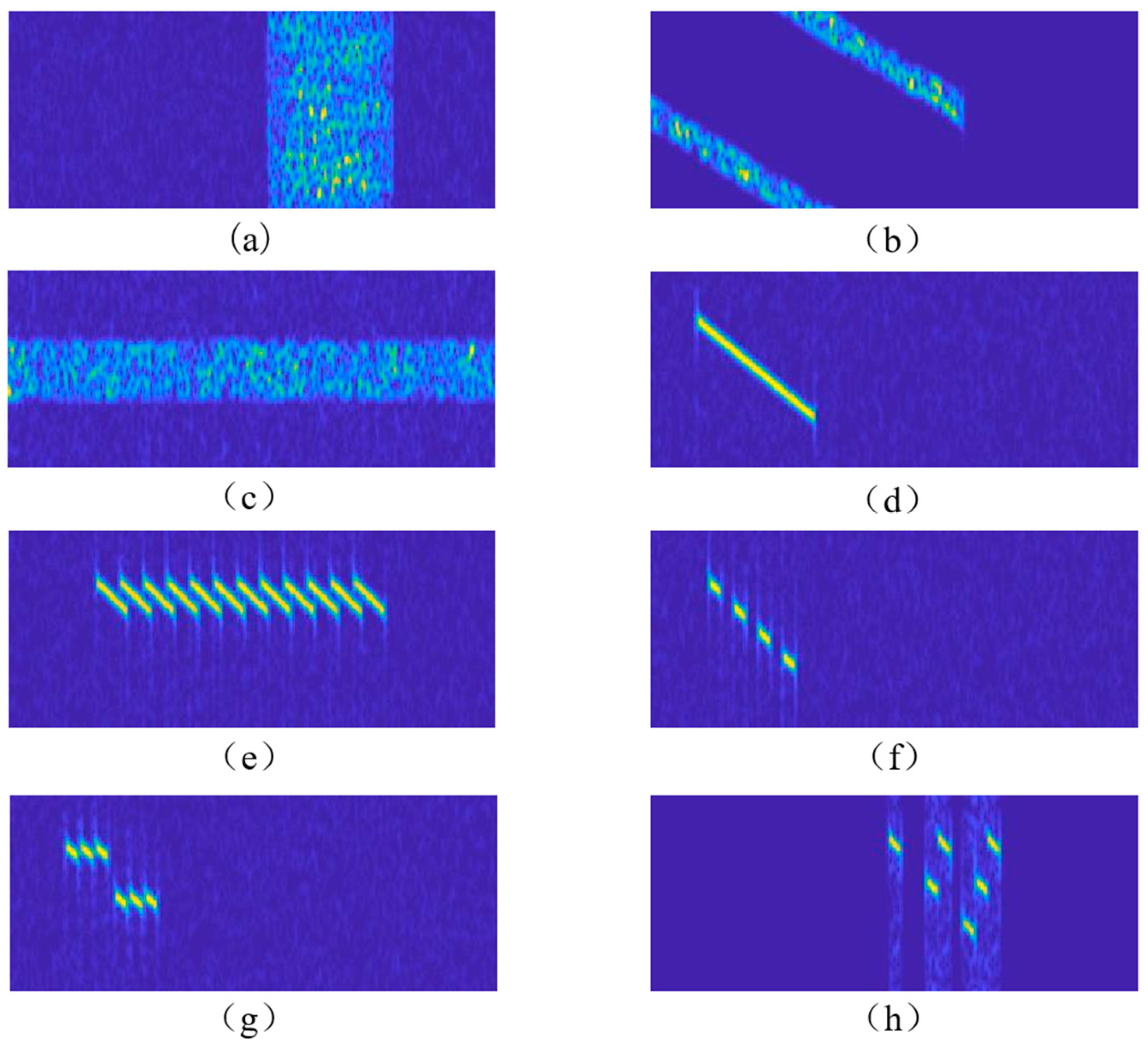
2.1. Noise Convolution Jamming

NCJ is a convolution modulation jamming based on DRFM technology. It convolves the received radar pulse signal with noise and sends it out after modulation and amplification, causing the radar to be subjected to both suppression and deception effects. The signal model of NCJ can be represented as follows:

$$J_{NCJ}(t)=A\cdot rect({\displaystyle \frac{t-T_{SM}}{T_{SM}}})s(t-T_{SM})\ast n(t)$$

(1)

where $s(t)$ represents the radar transmitted linear frequency modulation (LFM) signal, $A$ is the amplitude of the modulated jamming, $T_{SM}$ is the width of the intercepted slice, $n(t)$ is Gaussian white noise with length $T_{SM}$, and the symbol $‘\ast ’$ represents convolution operation.

2.2. Swept Jamming

SJ is a typical suppression jamming technology. It generates a broadband signal with a frequency that continuously changes over time to cover the radar’s operating frequency band, thereby blocking the radar from receiving and processing normal signals. Its core lies in using noise to modulate the carrier frequency, while making the central frequency of the entire frequency-modulated signal scan according to certain rules, thus possessing the dual characteristics of broadband noise suppression and frequency scanning coverage. The signal model of SJ can be represented as follows:

$$J_{SJ}(t)=A\cdot \cos \left[2\pi (f_{j}t+{\displaystyle \frac{\mu }{2}}{t}^2+k{\displaystyle {\int }_0^{t}n(\tau )}d\tau )+{\phi }_0\right]$$

(2)

where $f_j$ is the initial center frequency; $\mu$ represents the linear change rate of the center frequency; $k$ represents the frequency-modulation index, which determines the instantaneous spectrum width of the noise frequency modulation; $n(t)$ represents Gaussian white noise; and ${\phi }_0$ represents the initial phase.

2.3. Aiming Jamming

AJ is a kind of precise suppression jamming. It affects the detection of target echoes within the passband of the radar receiver by generating jamming signals that coincide with the radar frequency. This jamming mode features concentrated jamming frequencies, allowing all jamming energy to be used for suppressing radar signals. However, it imposes high requirements on the jammer, which needs to be guided to the jamming frequency through specific reconnaissance. The signal model of AJ can be represented as follows:

$$J_{AJ}(t)=A\cdot \cos \left[2\pi f_{0}t+k{\displaystyle {\int }_0^{t}n(\tau )d\tau +{\phi }_0}\right]$$

(3)

where $f_0$ is the carrier frequency.

2.4. Full Pulse Forwarding Jamming

FPFJ intercepts the entire radar pulse signal through a DRFM. After a certain amount of amplification and delay, it is forwarded and generates false targets near the real target. Since full pulse repeater jamming can completely preserve the characteristics of the radar signal, the generated false targets have extremely high coherence, often making it difficult for the radar to distinguish, thus resulting in false detection and tracking of the target. The signal model of FPFJ can be represented as follows:

$$J_{FPFJ}(t)=A\cdot \exp \left\{2\pi j\left[f_0(t-t_0)+{\displaystyle \frac{k}{2}}{(t-t_0)}^2+{\phi }_0\right]\right\}$$

(4)

where $t_0$ is the forward delay of the DRFM.

2.5. Mono-Pulse Dense Forwarding Jamming

MDFJ [32] intercepts only part of the radar signal for replication through DRFM and forwards it multiple times to form a dense false target group at the radar receiver. Although this jamming can only obtain partial radar gain, the large number of forwarding slices endows it with a certain suppression effect. The signal model of MDFJ can be represented as follows:

$$J_{MDFJ}(t)=A\cdot {\displaystyle \sum _{m=0}^{M-1}rect\left(\frac{t-T_1-m\tau -T_s/2}{T_s}\right)}s\left(t-T_1-m\tau \right)$$

(5)

where $T_S$ is the length of the signal intercepted by the jammer, $T_1$ is time delay of the first false target relative to the real target, $\tau$ represents the forwarding interval starting from the second forwarding, and $M$ is the number of false targets.

2.6. Interrupted Sampling and Direct Repeater Jamming

After the jammer detects the radar signal, ISDRJ intermittently samples the signal with a fixed slice width, stores the samples, and directly forwards them after simple processing, forming a group of false targets with uniform intervals. The signal model of ISDRJ can be represented as follows:

$$J_{ISDRJ}(t)=A\cdot {\displaystyle \sum _{n=0}^{N-1}rect\left(\frac{t-T_1-n{T}_c-T_s/2}{T_s}\right)}s\left(t-T_1\right)$$

(6)

where $N$ is the number of sampling times, and $T_c$ is the sampling period.

2.7. Interrupted Sampling and Periodic Repeater Jamming

ISPRJ is formed by multiple repeated forwarding on the basis of ISDRJ and has a better jamming effect. Its signal model can be represented as follows:

$$J_{ISPRJ}(t)={\displaystyle \sum _{m=0}^{M-1}{\displaystyle \sum _{n=0}^{N-1}rect\left(\frac{t-T_1-n{T}_c-m\tau -T_s/2}{T_s}\right)}}s\left(t-T_1-m\tau \right)$$

(7)

2.8. Interrupted Sampling and Cyclic Repeater Jamming

ISCRJ not only forwards the currently intercepted signal segment but also forwards all previously intercepted and stored signal segments in reverse order. Compared with ISDRJ and ISPRJ, the false targets of ISCRJ after pulse compression are distributed over a wider range and in a more irregular pattern, which makes it more difficult for the radar to counter jamming and detect targets. The signal model of ISCRJ can be represented as follows:

$$J_{ISCRJ}(t)={\displaystyle \sum _{m=0}^{M-1}{\displaystyle \sum _{r=0}^{R-1}rect\left(\frac{t-T_1-r{T}_c-m\tau -T_s/2}{T_s}\right)}}s(t-T_1-m{T}_c-m\tau )$$

(8)

where $R=\min \left\{N_c,M\right\}$ represents the number of forwarding times, $N_c=⌈T/T_c⌉$, $T$ is the pulse width, and $⌈\cdot ⌉$ denotes the ceiling function.

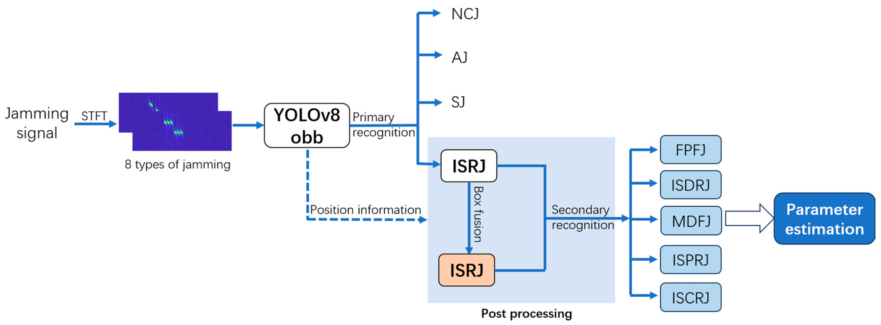
3. The Proposed Method

In this section, the proposed method of active jamming recognition and parameter estimation based on YOLOv8 is described in detail and whose main process is shown in Figure 1. Specifically, it consists of four parts: data preprocessing, YOLOv8-OBB, post-processing, and parameter estimation.

Figure 1. Flowchart of the proposed method.

3.1. Data Preprocessing

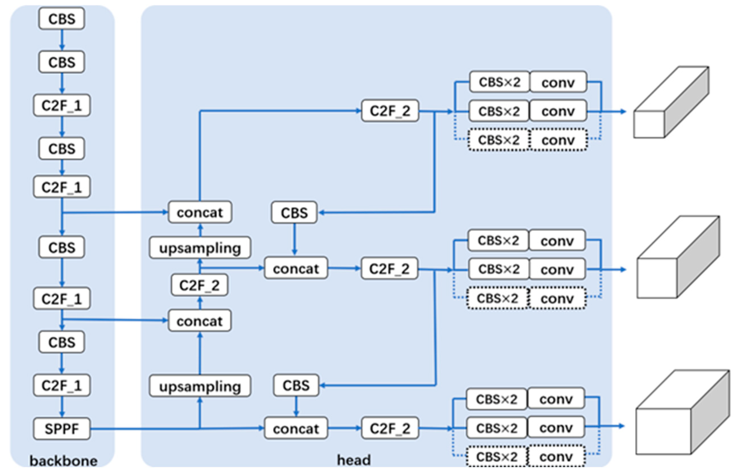
For the jamming signals received by radar, this paper employs the Short-Time Fourier Transform (STFT) for data preprocessing [33]. As a widely used time–frequency analysis method, the core concept of STFT is to divide a non-stationary signal into numerous short time segments through windowing on the basis of the Fourier transform. Within each short segment, the signal is considered approximately stationary, after which the correlation between the time domain and frequency domain within the segment is analyzed. The calculation formula of STFT is as follows:

$$W_d[n,k]={\displaystyle \sum _{m=-\infty }^{+\infty }{x}_d(m){\omega }^{\ast }(m-n)e^{-j\frac{2\pi }{N_k}kn}}$$

(9)

where $\omega (m-n)$ represents the window function, $x_d(m)$ represents the discrete input signal at sample index $m$, $n$ is the time index, $k$ is the frequency index, $N_k$ is the number of frequency sampling points, and $‘\ast ’$ denotes the complex conjugate.

For the time–frequency spectrogram obtained by STFT, the brightness or color of the image represents the energy or amplitude of the jamming at the corresponding time and frequency. By observing the changes in the frequency components of different jamming signals over time and extracting the visual features of the image as the input to the deep learning network, subsequent jamming detection can be carried out. In this paper, the STFT employs a Hamming window with a window length of 32 points, an overlap of 24 points, and 128 FFT points to generate a two-dimensional time–frequency spectrogram with the sampling frequency of 20 MHz and the pulse repetition time of 100 us, and the resolution of images are 156 × 386. The spectrogram examples of the eight types of jamming are shown in Figure 2.

Figure 2. The time–frequency spectrograms of the eight types of jamming. (a) NCJ (JNR = 10 dB). (b) SJ (JNR = 45 dB, sweep frequency cycle = 60 us, sweep bandwidth = 20 MHz). (c) AJ (JNR = 10 dB). (d) FPFJ (JNR = 10 dB, bandwidth = 12 MHz, pulse width = 25 us). (e) MDFJ (JNR = 10 dB, forward period = 3 us, forward times = 12). (f) ISDRJ (JNR = 10 dB, slice number = 4). (g) ISPRJ (JNR = 10 dB, slice number = 2, forward period = 2 us, forward times = 3). (h) ISCRJ (JNR = 10 dB, sampling times = 3, sampling period = 4 us).

3.2. YOLOv8 OBB

YOLOv8 is an advanced object detection algorithm in the field of computer vision, integrating various learning tasks such as detection, segmentation, classification, and pose estimation. As a sub-algorithm within it, OBB is used to achieve oriented object detection. Its network structure is shown in Figure 3. The network mainly consists of two parts: the backbone and the head. The backbone network is used for down-sampling and feature extraction of the input data. The head part mainly splices and fuses feature maps through up-sampling and residual connections and predicts the detection boxes, object categories, and the angles of the oriented detection boxes in three branches of different scale sizes at the output part. Considering the limited length of this article, only the structure of YOLOv8 is briefly introduced, with details available in [34].

Figure 3. YOLOv8 OBB network structure.

In the proposed method, when the YOLOv8 OBB network detects jamming time–frequency spectrograms, it classifies all slices of ISRJs into a single category and conducts preliminary recognition between ISRJs and the three types of suppression jamming. The network output includes two-dimensional position information in both time and frequency domains, enabling the classification of four jamming types: ISRJ, AJ, SJ, and NCJ.

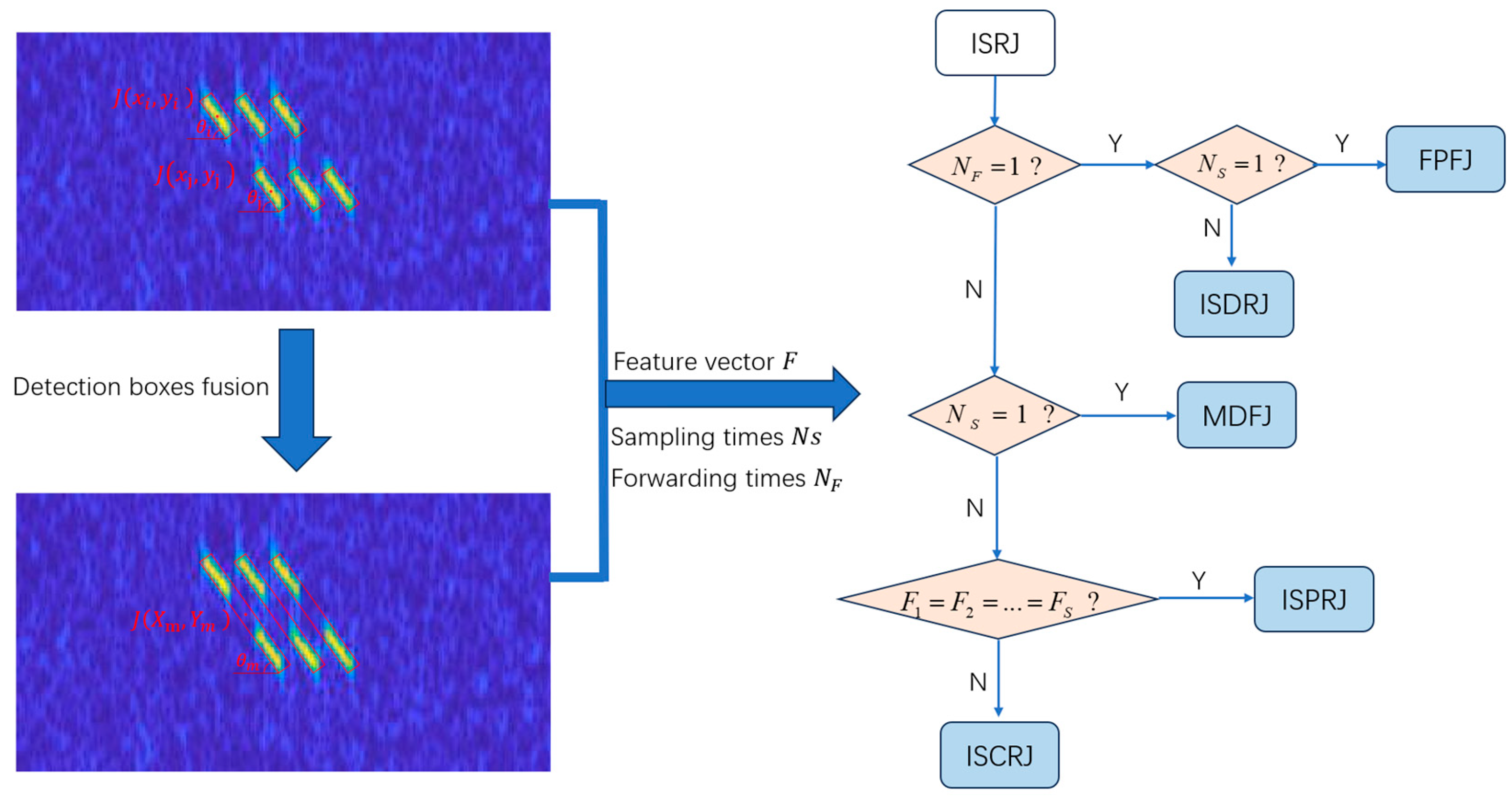
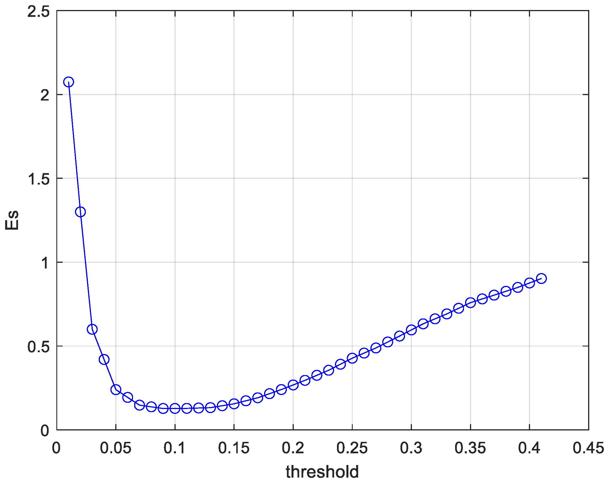
3.3. Post-Processing Algorithm

After detecting the jamming time–frequency spectrogram through the OBB network, a post-processing algorithm is added to the end of the network to carry out further secondary recognition for ISRJ and provide necessary conditions for the subsequent estimation of different ISRJ parameters. The specific process is shown in Figure 4.

Figure 4. Post-processing algorithm flowchart.

The post-processing is mainly divided into two parts: feature extraction and secondary recognition. The first part performs detection box fusion on ISRJ through the slope matching method, which is used to merge different slices under the same forwarding with one object. The specific process is described as follows:

The output of the network contains the position information $\left(x,y\right)$ and the frequency-modulation slope information $\theta$ of the jamming signal in the time–frequency spectrogram. For jamming slice $J(x_i,y_i)$ with the angle of ${\theta }_i$, traverse the remaining slices $J(x_j,y_j)$ with the angle of ${\theta }_j$, if the following condition is satisfied:

$$\left|-{\displaystyle \frac{1}{n}}{\displaystyle \sum _{k=1}^n\tan {\theta }_k-\frac{y_i-y_j}{x_i-x_j}}\right|\le \eta$$

(10)

where $n$ is the total number of jamming slices, and $\eta$ is the judgment threshold (the specific value of $\eta$ will be discussed in Section 4).

Then, the two jamming slices are determined to belong to the same forwarding and are fused into a whole slice $J(x_f,y_f)$ with the angle of ${\theta }_f$, where $X_m=\left(x_i+x_j\right)/2$, $Y_m=\left(y_i+y_j\right)/2$, and ${\theta }_m=-\arctan \left[(y_i-y_j)/(x_i-x_j)\right]$. After traversing all slices in the jamming sample, the fused detection box contains all the jamming slices under the same forwarding and outputs the vector of parameter feature $S=\left(F_1,F_2,\cdots ,F_m,\cdots \right)$, which represents the number of jamming slices under different forwarding times. The specific process is shown in Algorithm 1.

Algorithm 1. Procedures of detection box fusion

Input: Detection boxes information $W=\left\{\left(x_1,y_1,{\theta }_1\right),\left(x_2,y_2,{\theta }_2\right),\cdots ,\left(x_n,y_n,{\theta }_n\right)\right\}$ and the threshold $\eta$.

Output: Parameter feature vector $S=\left(F_1,F_2,\cdots ,F_m,\cdots \right)$. While $W$ is not empty, $W1=\left(x_i,y_i,{\theta }_i\right)$, $W2=setdiff(W,W1)$, where $x_i$ is the minimum value of the horizontal axis in $W$, $setdiff()$ returns the set of difference. Otherwise, terminate the algorithm. For each element in $W2$, if its calculation result with $W1$ satisfies Equation (10), then $W3=\left\{(x,y,\theta )\in W2\left| \mathrm{Equation} \left(10\right) \mathrm{holds} \mathrm{for} (x,y,\theta )\right.\right\}$. Let $N$ denote the number of elements in $W3$ at the $m$-th cycle, then $F_m=N+1$. Update $W=setdiff(W,W3+W1)$ and return to Step 1.

According to the algorithm results, the number of forwarding times $N_F$ is obtained based on the quantity of elements in the feature vector $S$, and the number of sampling times $N_S$ is obtained based on the maximum value of the elements in the feature vector $S$, thereby proceeding with subsequent secondary recognition.

In the second part, logical judgment is carried out based on the extracted features: $N_F$, $N_S$, and $S$. When $N_F=1$ and $N_S=1$, it is determined as FPFJ; when $N_F=1$ and $N_S>1$, it is determined as ISDRJ; when $N_F>1$ and $N_S=1$, it is determined as MDFJ; when $F_1=F_2=\dots =F_S$, it is determined as ISPRJ; when $F_1\ne F_2\ne \dots \ne F_S$, it is determined as ISCRJ. Thus, the secondary recognition of 5 types of ISRJ is achieved.

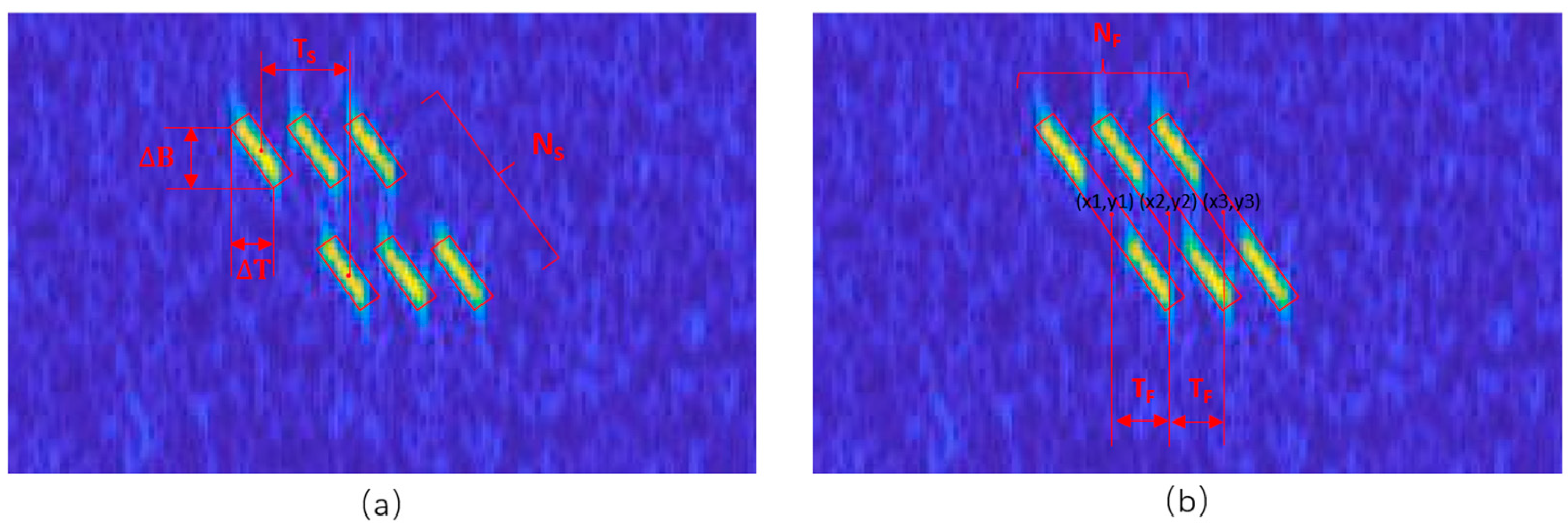
3.4. Parameter Estimation

For the five types of ISRJ, by combining the detection box information output from the network, the key feature obtained from detection box fusion, and the results of secondary recognition, all parameters of different ISRJ can be estimated. For the time width $\Delta T$ and bandwidth $\Delta B$ of the slice, their estimation is directly carried out through the detection box information; for the sampling times $N_S$ and forwarding times $N_F$, they can be obtained through feature vector $S$; for the forwarding period $T_F$, it can be estimated by computing the average interval of the fused boxes; and for the sampling period $T_S$, the estimation can be made by computing the interval between slices within the same forwarding.

Since ISPRJ includes the estimation process for all parameters, and the parameter estimation processes for the remaining four types of ISRJs are basically the same as that of ISPRJ, we take ISPRJ as an example for analysis whose parameter calculation process is shown in Figure 5. Additionally, $N_S$ and $N_F$ have already been estimated in the post-processing algorithm section, thus we mainly elaborate on the estimations of $\Delta T$, $\Delta B$, $T_S$, and $T_F$.

Figure 5. Parameter estimation of ISPRJ. (a) Before fusion of detection boxes. (b) After fusion of detection boxes.

The bandwidth $\Delta B$ and time width $\Delta T$ are calculated by

$$\Delta B=h\cdot \sin (\theta )\cdot f_s/S_{tfw}$$

(11)

$$\Delta T=h\cdot \cos (\theta )\cdot T_{PRT}/S_{tfh}$$

(12)

where $h$ is the height of the detection box,$\theta$ is the angle of the detection box, $f_s$ is the sampling frequency, $T_{PRT}$ is the pulse repetition period, and the resolution of the time–frequency spectrogram is $S_{tfw}\times S_{tfh}$.

The sampling period $T_S$ is calculated by

$$T_S={\displaystyle \frac{T_{PRT}}{S_{tfw}}}\cdot {\displaystyle \frac{1}{M\left(N-1\right)}}{\displaystyle \sum _{m=1}^M{\displaystyle \sum _{n=1}^{N-1}\left|x_{m,n}-x_{m,n+1}\right|}}$$

(13)

where $x_{m,n}$ represents the horizontal axis coordinate of the center of the $n$-th slice under the $m$-th forwarding before fusion.

The forwarding period $T_F$ is calculated by

$$T_F={\displaystyle \frac{T_{PRT}}{W}}\cdot {\displaystyle \frac{1}{M-1}}{\displaystyle \sum _{m=1}^{M-1}\left|X_m-X_{m+1}\right|}$$

(14)

where $X_m$ represents the horizontal axis coordinate of the center of the $m$-th forwarding after fusion.

4. Simulation Experiment and Result Analysis

In this section, the conditions of the simulation experiment and other relevant settings are introduced in detail. Then, the results of simulation experiments are analyzed, and the parameter estimation results are compared with those in existing relevant literature.

4.1. Experimental Conditions

4.1.1. Jamming Simulation

In the experiments of this paper, jamming simulations are employed to generate the training data required by the network. Additionally, to mitigate network overfitting and enhance the reliability and generalization of experimental results, most adjustable parameters of the jamming signals are set to vary randomly within specific ranges—this helps adapt to the complex environment of radar electronic countermeasures. The specific parameter settings are detailed in Table 1.

Table 1. Simulation parameters for eight types of jamming.

Jamming Types	Parameters	Value Range
NCJ	JNR	0~20 dB
SJ	JNR Sweep frequency cycle Sweep bandwidth	30~60 dB 40~80 us 20 MHz
AJ	JNR	0~20 dB
FPFJ	JNR Bandwidth Pulse width	0~20 dB 5~15 MHz 10~25 us
MDFJ	JNR Forward period Forward times Duty	0~20 dB 2~5 us 8~12 35%~45%
ISDRJ	JNR Slice number Duty	0~20 dB 2~4 45%~60%
ISPRJ	JNR Slice number Forward period Forward times Duty	0~20 dB 2~3 2~3 us 2~4 45%~60%
ISCRJ	JNR Sampling times Sampling period	0~20 dB 2~3 1.875~5 us

4.1.2. Dataset Construction

During network training, according to the parameter value ranges of the above eight types of jamming, 1000 training samples and 200 validation samples are randomly generated for each type, forming a training dataset with a total of 9600 samples. During network testing, 1000 samples are respectively generated for each of the eight types of jamming under different JNRs, which are used for subsequent recognition and ISRJ parameter estimation.

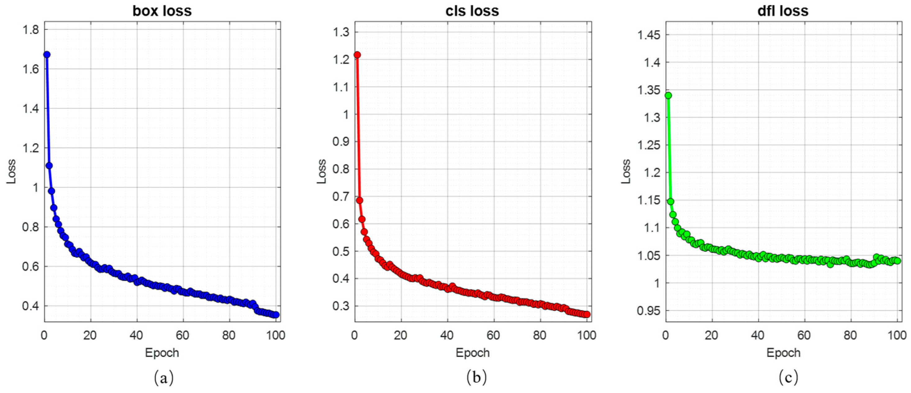
4.1.3. Training of the Network

For the jamming time–frequency spectrograms generated by simulation, they are first cropped to 416 × 416 pixels and input into the OBB network. During the network training process, this paper employs the YOLOv8n model with the best real-time performance, sets the batch size to 4, the number of training epochs to 100, the training confidence to 0.001, and uses the Adamw optimizer with a learning rate of 0.002. The loss functions include BCE Loss and CIOU Loss. Mosaic augmentation is disabled for the last 10 epochs during the later stage of training.

In addition, the computer system used in this experiment is Windows 11, with 8 GB of RAM, an NVIDIA GeForce RTX 1650 GPU, and Python version 3.8.

4.2. Simulation and Result Analysis

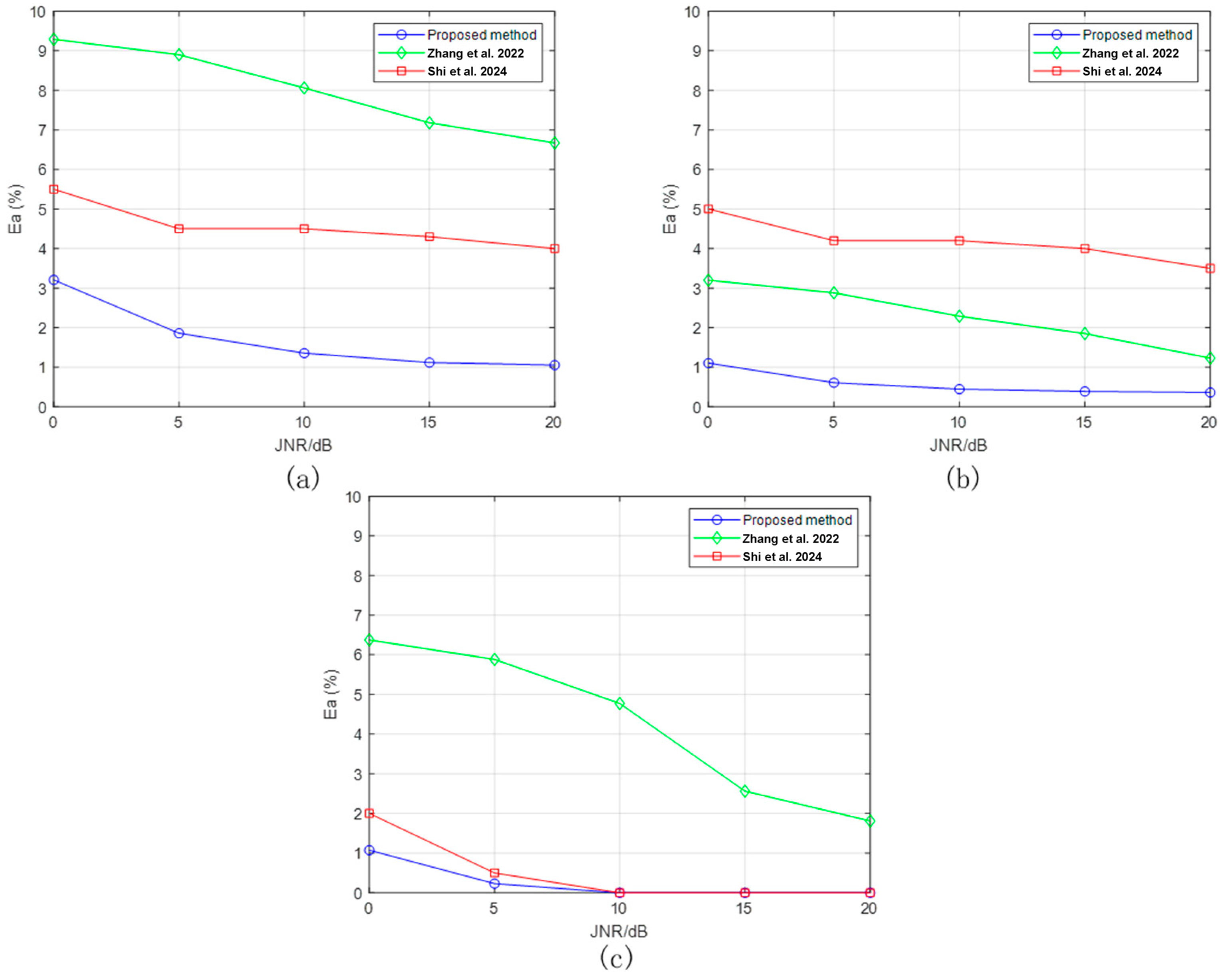
4.2.1. Error Simulation Experiment

In the post-processing algorithm in Section 3, we use a threshold $\eta$ to achieve the fusion of detection boxes; the value of $\eta$ is determined through the following experiment. Since the output of the post-processing algorithm is a one-dimensional vector $S=\left[F_1,F_2,\dots ,F_m,\dots ,F_S\right]$, we can calculate the error $E_S$ between the actual $S$ and the output $\widehat{S}$ of the post-processing algorithm and select the value of $\eta$ when the average of $E_S$ is the smallest as the final threshold in this experiment. The calculation of $E_S$ is defined by the L1 distance, expressed as follows:

$$E_S={\displaystyle \frac{1}{L}}{\displaystyle \sum _{l=1}^L\left|S_l-{\widehat{S}}_l\right|}$$

(15)

where $L$ represents the number of samples under different values of $\eta$. In the experiment, $L=1000$.

The experimental results of the error simulation are shown in Figure 6. When the value of $\eta$ is around 0.12, $E_S$ is in a stable state and has the minimum average value. Since the fluctuation of $E_S$ here is relatively small, and its error is negligible, $\eta =0.12$ can be directly adopted.

Figure 6. Error simulation experiment of the threshold $\eta$.

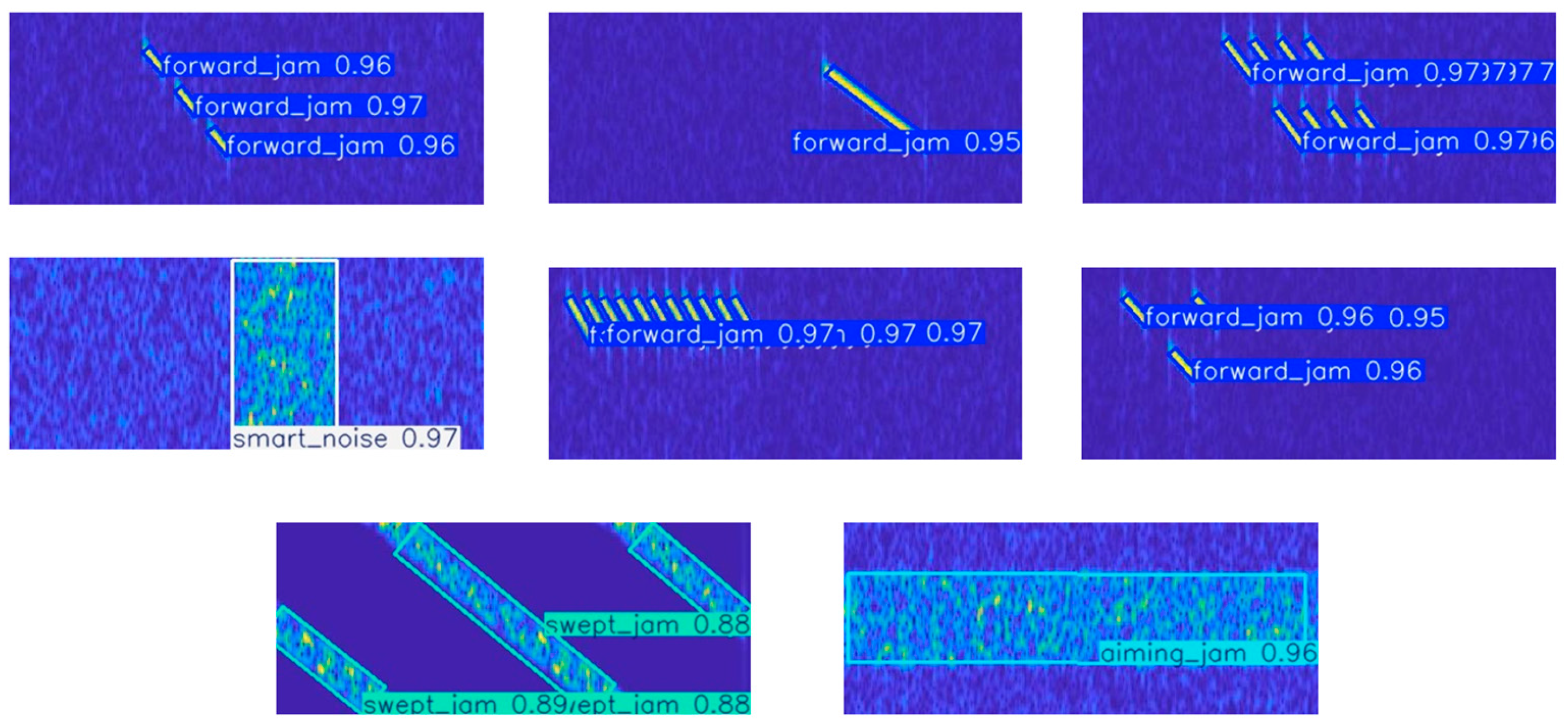
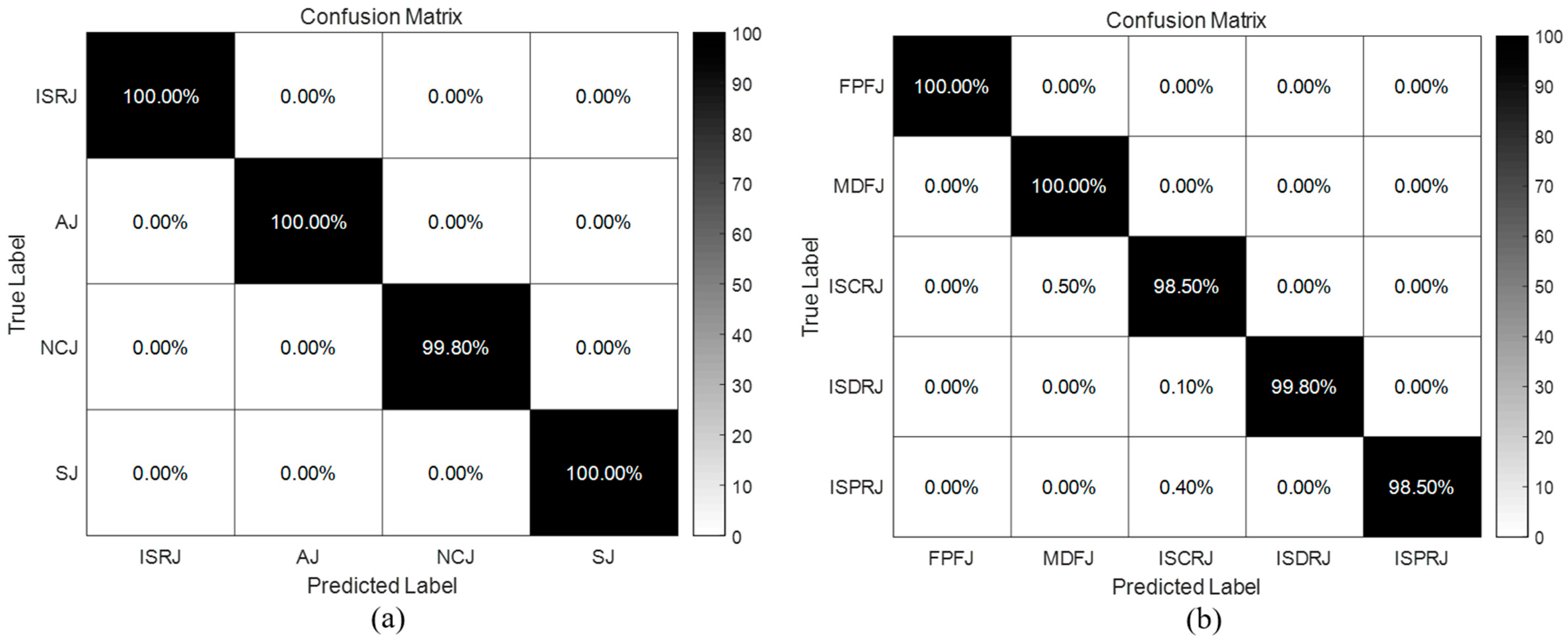
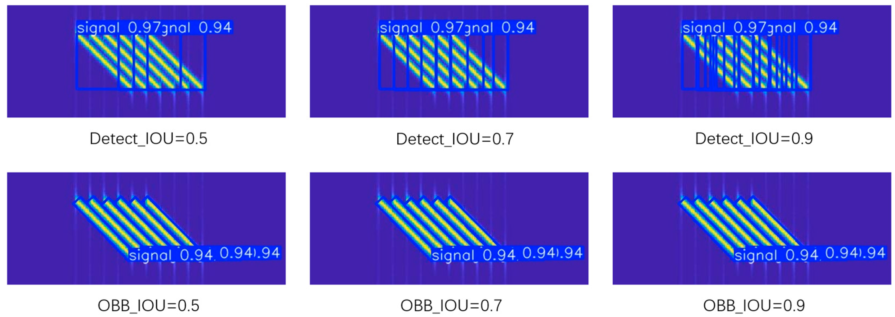
4.2.2. Analysis of Detection and Recognition Results

When the test dataset containing eight types of jamming is input, the OBB network first conducts detection and primary recognition after training. Subsequently, the post-processing algorithm performs secondary recognition for ISRJ. The box loss, classification loss, and distribution focal loss curves of the training set are presented in Figure 7, and the detection and recognition results are presented in Figure 8 and Figure 9, respectively.

Figure 7. Three types of loss curves. (a) Box loss curve. (b) Classification loss curve. (c) Distribution focal loss curve.

Figure 8. OBB network detection results.

Figure 9. Recognition results. (a) Primary recognition result. (b) Secondary recognition result.

In Figure 7, we can observe that the three loss curves generally show a decreasing trend during the training process. In the last 10 epochs of training, the mosaic augmentation was disabled, allowing the network to focus more on learning the details of the original images, thus further reducing the box loss and classification loss. Meanwhile, due to the significant change in the network input, the distribution focal loss fluctuated to some extent but eventually stabilized.

We see from Figure 9a that both ISRJ and the three types of suppression jamming demonstrate good recognition performance. Among them, the correct recognition probabilities of ISRJ, AJ, and SJ all reach 100% under the condition of 0~20 dB. Only a few samples of SNJ were not detected by the network due to low JNR, which reduced recognition probability slightly. We see from Figure 9b that FPFJ and MDFJ achieved a 100% recognition rate, while for ISCRJ, ISDRJ, and ISPRJ, the misrecognition of individual samples was caused by the failure of detection boxes fusion for a small number of samples during post-processing. Overall, both primary and secondary recognition achieved correct rates exceeding 98.5%.

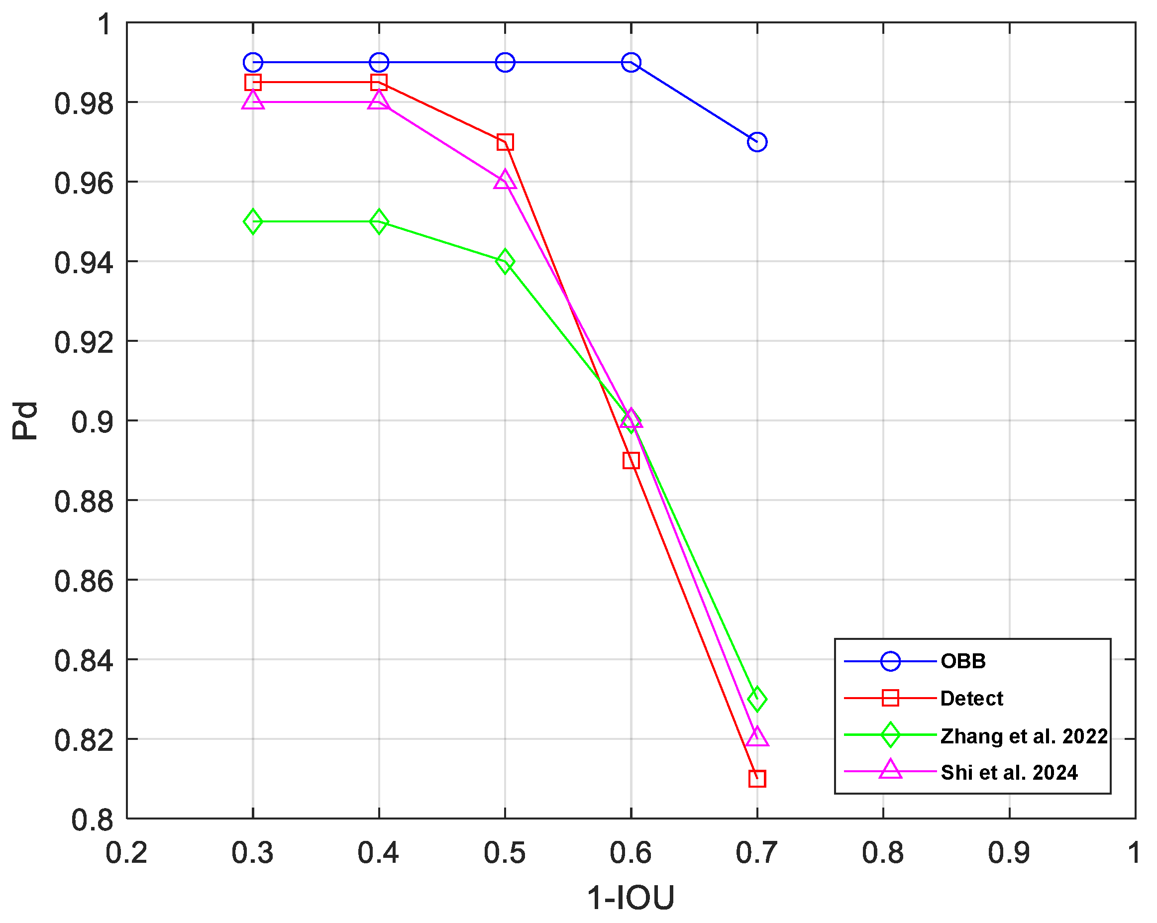
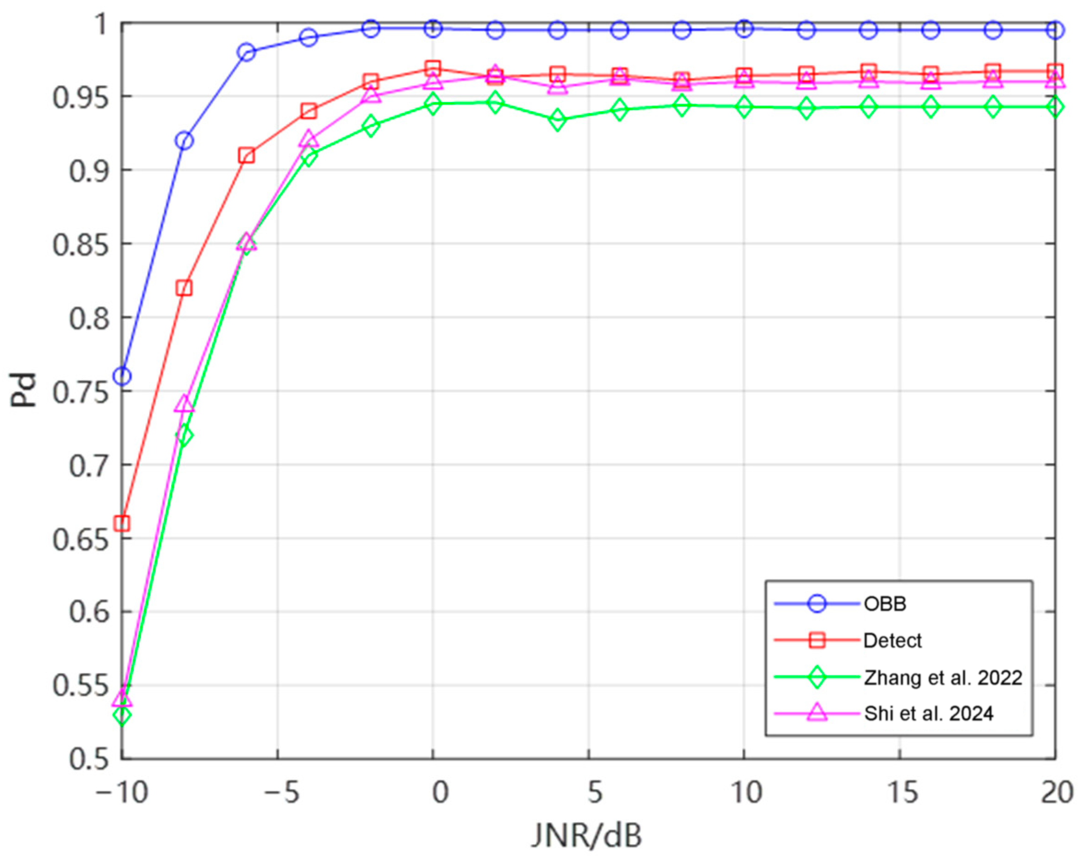
4.2.3. NMS and the Result of Detection Probability

NMS is a classic algorithm in object detection for eliminating redundant detection boxes [35], with its core idea being the following: retaining local maximum values and suppressing non-maximum values. In practical applications, it filters out candidate boxes with excessively high overlap rates, ensuring that each object outputs only one optimal detection result. For dense forwarding jamming signals, the oriented bounding box detection network (OBB) and the horizontal bounding box detection network (Detect) under the YOLOv8 structure were used for detection, and the results are shown in Figure 10.

Figure 10. Detection performance of Detect and OBB networks at different IOU thresholds.

We see that when the IOU threshold is small (e.g., Detect-IOU = 0.5), the NMS algorithm mistakenly suppresses the correctly detected bounding boxes, leading to missed detections. When the IOU threshold is large (e.g., Detect-IOU = 0.9), multiple overlapping bounding boxes will appear for the same forwarding jamming, causing false alarms. Therefore, for forwarding jamming with different densities, it is necessary to set different IOU thresholds to achieve better detection effects (e.g., Detect-IOU = 0.7), which is difficult to implement in complex and changeable environments.

For oriented detection models, since their detection boxes fit more closely to the boundaries of jamming, they can effectively avoid the missed detection and false alarm problems caused by the IOU threshold (e.g., OBB-IOU = 0.5, 0.7, 0.9), that is, the density of jamming distribution has little effect on the detection results.

To intuitively demonstrate the advantages of oriented bounding box detection, we compare the OBB method, the Detect method, the method in [26], and the method in [27] through ablation experiments under different IOU thresholds. The method in [26] is a horizontal bounding box detection based on YOLOv5, and the method in [27] is a horizontal bounding box detection based on YOLOv7-tiny. With the vertical axis being the probability of detection (Pd), the results in Figure 11 show that for jamming with a certain density, the four methods all have good detection probabilities under higher IOU thresholds. However, when the IOU threshold decreases, the Pd of the three horizontal bounding box detection methods decreases rapidly, but the OBB method is less affected and still maintains a high Pd. This simulation result not only verifies the correctness of the NMS analysis but also proves that the OBB method has more advantages in dealing with complex and changeable jamming.

Figure 11. The curve of Pd versus IOU for the four methods [26,27].

To further investigate the impact of different JNRs on the Pd, we conducted experiments under the commonly used IOU threshold of 0.5, and the results are shown in Figure 12. Comparing the four methods, the OBB method demonstrates higher detection probabilities across both low and high JNR conditions. During training, the OBB network’s annotation information aligns more precisely with the time–frequency signals of jamming sources, enabling the extraction of more concentrated and accurate features. In contrast, the Detect network’s annotations include not only the jamming signals but also a large amount of background noise. Therefore, the OBB has a higher detection probability in low JNR scenarios. In high JNR environments, the NMS algorithm becomes the dominant factor affecting detection performance. In this case, the OBB network maintains its superiority in detecting partially dense repeater jamming, leading to consistently higher detection probabilities.

Figure 12. The curve of Pd versus JNR when IOU = 0.5 [26,27].

4.3. Analysis of Parameter Estimation Results

In the experiments of this paper, the estimation error of parameters is measured by $E_r$, which can be expressed as

$$E_r={\displaystyle \frac{\left|P_m-{\tilde{P}}_m\right|}{P_m}}$$

(16)

where $P_m$ and ${\tilde{P}}_m$ represent the true value and the estimated value of the parameter, respectively.

In the testing phase, the samples in the test dataset are sequentially fed into the OBB network and the post-processing algorithm. After parameter estimation performed based on the detection box information, the average estimation errors of the parameters for each of the five types of ISRJ under the JNR of 0~20 dB are presented in Table 2. Different sampling and forwarding mechanisms lead to differences in parameter estimation accuracy. From the estimation results of $\Delta T$ and $\Delta B$, it can be seen that the longer the jamming sampling segment and the higher the duty cycle, the more accurate the fitting of the slices by the detection boxes output by the network, and the smaller the average estimation errors of these two parameters. For $N_S$ and $N_F$, since they are related to the number of times and have a high correlation with the detection probability, their average estimation errors are both lower than 0.9% and generally smaller than those of other parameters. For $T_S$ and $T_F$, these two parameters are estimated after bounding box fusion; therefore, the estimation results are strongly correlated with the estimation of $N_S$ and $N_F$. That is, under the premise of correct estimation of $N_S$ and $N_F$, the average error of $T_S$ and $T_F$ remains a relatively low level of around 1%. Overall, the average estimation errors of the above six types of parameters by the method in this paper are all lower than 1.85%, indicating a relatively high estimation accuracy.

Table 2. The average error of six parameters at JNR of 0–20 dB.

	$\mathbf{\Delta }\mathit{T}$	$\mathbf{\Delta }\mathit{B}$	${\mathit{T}}_{\mathit{S}}$	${\mathit{N}}_{\mathit{S}}$	${\mathit{T}}_{\mathit{F}}$	${\mathit{N}}_{\mathit{F}}$
FPFJ	1.398%	1.477%	-----	0	-----	0
MDFJ	0.879%	0.871%	-----	0	1.120%	0.021%
ISDRJ	1.542%	1.808%	0.577%	0.075%	-----	0.300%
ISPRJ	1.289%	1.542%	0.464%	0.433%	0.844%	0.167%
ISCRJ	1.857%	1.772%	0.669%	0.633%	-----	0.900%

Figure 13 shows the comparison results of the estimation accuracy of three parameters with the methods in [26,27]. Among them, $E_a$ represents the average estimation error of the same parameter under 5 types of ISRJ. It can be seen that the parameter estimation accuracy of the three methods continuously improves as the JNR increases. However, the parameter estimation error of the method proposed in this paper always remains a lower level, within the range of 0~20 dB. On one hand, this is due to the detection performance advantage of YOLOv8, and on the other hand, it is because the annotation method of the oriented bounding boxes makes the network extract jamming features more concentratedly and accurately.

Figure 13. The variation curve of $E_a$ with JNRs for three parameters. (a) The comparison of the slice width. (b) The comparison of the sampling period. (c) The comparison of the sampling times [26,27].

5. Discussion

From the comparison between the simulation results and existing methods in Sec-tion 4, it can be seen that when facing ISRJ, the proposed method has good advantages in both jamming detection and jamming parameter estimation processes. Moreover, for some other radar jamming, such as smeared spectrum jamming, the proposed method is also applicable, thus it has a certain generalization performance. However, the method in this paper also has problems and challenges that need to be further solved. For example, there are correlations among different parameters during the estimation process, and they cannot be calculated independently, which imposes certain constraints on the parameter estimation process.

6. Conclusions

Based on the idea of oriented object detection, this paper has proposed a new method for jamming recognition and parameter estimation. The OBB network is used for primary recognition and outputs the jamming detection information; then, the post-processing algorithm is used for secondary recognition of ISRJ and assists in subsequent parameter estimation. Different from traditional perception methods, this paper applies oriented bounding box detection to the jamming field. Through simulation and analysis under different NMS conditions, the detection advantages of the proposed method under dense distributed forwarding jamming are verified. This advantage enables the network to have a relatively high jamming detection probability under both low and high JNRs. In addition, through the OBB network and the post-processing algorithm, the correct probability of primary recognition for 8 types of jamming in this paper reaches more than 99.8%, and the correct probability of secondary recognition reaches more than 98.5%. In terms of parameter estimation, the average estimation error of the proposed method for 6 parameters of 5 types of ISRJ is less than 1.85%. Compared with existing methods, it has higher estimation accuracy under different JNRs.

References

- Johnston, S.L. Radar electronic counter-countermeasures. IEEE Trans. Aerosp. Electron. Syst. 2007, 14, 109–117. [Google Scholar] [CrossRef]
- Orlando, D. A novel noise jamming detection algorithm for radar applications. IEEE Signal Process. Lett. 2016, 24, 206–210. [Google Scholar] [CrossRef]
- Feng, D.; Xu, L.; Pan, X.; Wang, X. Jamming wideband radar using interrupted-sampling repeater. IEEE Trans. Aerosp. Electron. Syst. 2017, 53, 1341–1354. [Google Scholar] [CrossRef]
- Kwak, C.M. Application of DRFM in ECM for pulse type radar. In Proceedings of the 2009 34th International Conference on Infrared, Millimeter, and Terahertz Waves, Busan, Republic of Korea, 21–25 September 2009. [Google Scholar]
- Lu, L.; Gao, M. An improved sliding matched filter method for interrupted sampling repeater jamming suppression based on jamming reconstruction. IEEE Sens. J. 2022, 22, 9675–9684. [Google Scholar] [CrossRef]
- Zheng, H.; Jiu, B.; Liu, H. Waveform design based ECCM scheme against interrupted sampling repeater jamming for wideband MIMO radar in multiple targets scenario. IEEE Sens. J. 2021, 22, 1652–1669. [Google Scholar] [CrossRef]
- Greco, M.; Gini, F.; Farina, A. Radar detection and classification of jamming signals belonging to a cone class. IEEE Trans. Signal Process. 2008, 56, 1984–1993. [Google Scholar] [CrossRef]
- Zhao, S.; Zhou, Y.; Zhang, L.; Guo, Y.; Tang, S. Discrimination between radar targets and deception jamming in distributed multiple-radar architectures. IET Radar Sonar Navig. 2017, 11, 1124–1131. [Google Scholar] [CrossRef]
- Yang, X.; Ruan, H. Active deception jamming identification method based on bispectrum analysis. J. Detect. Control. 2018, 40, 122–127. [Google Scholar]
- Zhou, H.; Dong, C.; Wu, R.; Xu, X.; Guo, Z. Feature fusion based on Bayesian decision theory for radar deception jamming recognition. IEEE Access 2021, 9, 16296–16304. [Google Scholar] [CrossRef]
- Liu, L.; Yang, H.; Xiao, G. Time-frequency domain feature extraction algorithm based on linear discriminant analysis. Syste. Eng. Electron. 2019, 41, 2184–2190. [Google Scholar]
- Tian, X.; Tang, B. Active deception jamming recognition of radar based on normalized wavelet decomposition power ratio. J. Data Acquisit. Process. 2013, 28, 416–420. [Google Scholar]
- Zhou, C.; Liu, Q.; Chen, X. Parameter estimation and suppression for DRFM-based interrupted sampling repeater jammer. IET Radar Sonar Navig. 2018, 12, 56–63. [Google Scholar] [CrossRef]
- Wang, C.; Wang, X.; Zhang, J. A novel parameter estimation method for ISRJ. In Proceedings of the 2nd International Conference on Electronic Materials and Information Engineering, Hangzhou, China, 15–17 April 2022. [Google Scholar]
- Geng, Z.; Yan, H.; Zhang, J.; Zhu, D. Deep-learning for radar: A survey. IEEE Access 2021, 9, 141800–141818. [Google Scholar] [CrossRef]
- Lv, Q.; Quan, Y.; Feng, W.; Sha, M.; Dong, S.; Xing, M. Radar deception jamming recognition based on weighted ensemble CNN with transfer learning. IEEE Trans. Geosci. Remote Sens. 2021, 60, 1–11. [Google Scholar] [CrossRef]
- Meng, Y.; Yu, L.; Wei, Y. Multiple information cognition of interrupted sampling repeater jamming in complex scenes. In Proceedings of the 2021 CIE International Conference on Radar (Radar), Haikou, China, 15–19 December 2021. [Google Scholar]
- Shao, G.; Chen, Y.; Wei, Y. Deep fusion for radar jamming signal classification based on CNN. IEEE Access 2020, 8, 117236–117244. [Google Scholar] [CrossRef]
- Shao, G.; Chen, Y.; Wei, Y. Convolutional neural network-based radar jamming signal classification with sufficient and limited samples. IEEE Access 2020, 8, 80588–80598. [Google Scholar] [CrossRef]
- Zhou, H.; Wang, L.; Guo, Z. Recognition of radar compound jamming based on convolutional neural network. IEEE Trans. Aerosp. Electron. Syst. 2023, 59, 7380–7394. [Google Scholar] [CrossRef]
- Gao, M.; Li, H.; Jiao, B.; Hong, Y. Simulation research on classification and identification of typical active jamming against LFM radar. In Proceedings of the Eleventh International Conference on Signal Processing Systems, Chengdu, China, 31 December 2019. [Google Scholar]
- Fan, P.; Wu, Y.; Wei, Y.; Guo, G.; Peng, Z. A method of jamming recognition based on multi-domain joint convolutional neural network. In Proceedings of the International Conference on Electronic Information Engineering and Computer Communication, Nanchang, China, 4 May 2022. [Google Scholar]
- Yu, X.; Wang, W.; Wu, H.; Bo, J.; Zhang, J.; Meng, J. Multi-domain feature fusion based radar deception jamming recognition method. In Proceedings of the 2023 IEEE 7th International Symposium on Electromagnetic Compatibility, Hangzhou, China, 20–23 October 2023. [Google Scholar]
- Luo, Z.; Cao, Y.; Yeo, T.S.; Wang, Y.; Wang, F. Few-shot radar jamming recognition network via time-frequency self-attention and global knowledge distillation. IEEE Trans. Geosci. Remote Sens. 2023, 61, 1–12. [Google Scholar] [CrossRef]
- Zhu, X.; Wu, H.; He, F.; Yang, Z.; Meng, J.; Ruan, J. YOLO-CJ: A Lightweight Network for Compound Jamming Signal Detection. IEEE Trans. Aerosp. Electron. Syst. 2024, 60, 6807–6821. [Google Scholar] [CrossRef]
- Zhang, J.; Liang, Z.; Zhou, C.; Liu, Q.; Long, T. Radar compound jamming cognition based on a deep object detection network. IEEE Trans. Aerosp. Electron. Syst. 2022, 59, 3251–3263. [Google Scholar] [CrossRef]
- Shi, Z.; Wu, H.; Zhu, X.; Wang, W.; Ni, X.; Zhang, J. Interrupted sampling forwarding jamming parameter estimation based on YOLOv7-tiny. In Proceedings of the 2024 IEEE 7th International Conference on Electronic Information and Communication Technology, Xi’an, China, 31 July–2 August 2024. [Google Scholar]
- Xie, A.; Liu, X.; Wu, Q.; Liu, Z.; Xiao, S. Recognition and Suppression of Slice Repeater Jamming Based on Coded Waveform. IEEE Trans. Aerosp. Electron. Syst. 2025, 61, 7466–7480. [Google Scholar] [CrossRef]
- Liu, X.; Wu, Q.; Pan, X.; Wang, J.; Zhao, F. SAR image transform based on amplitude and frequency shifting joint modulation. IEEE Sens. J. 2025, 25, 7043–7052. [Google Scholar] [CrossRef]
- Wu, Q.; Wang, Y.; Liu, X.; Gu, Z.; Xu, Z.; Xiao, S. ISAR Image Transform via Joint Intra pulse and Inter pulse Periodic coded Phase Modulation. IEEE Sens. J. 2025, in press. [Google Scholar] [CrossRef]
- Chen, L.; Wang, J.; Liu, X.; Feng, D.; Sun, G. A Flexible Range-Doppler Modulation Method for Pulse-Doppler Radar Using Phase-Switched Screen. IEEE Trans. Antennas Propag. 2025, in press. [Google Scholar] [CrossRef]
- Lv, Q.; Quan, Y.; Sha, M.; Feng, W.; Xing, M. Deep neural network-based interrupted sampling deceptive jamming countermeasure method. IEEE J.-STARS 2022, 15, 9073–9085. [Google Scholar] [CrossRef]
- Neemat, S.; Krasnov, O.; Yarovoy, A. An interference mitigation technique for FMCW radar using beat-frequencies interpolation in the STFT domain. IEEE Trans. Microw. Theory Tech. 2018, 67, 1207–1220. [Google Scholar] [CrossRef]
- Vijayakumar, A.; Vairavasundaram, S. Yolo-based object detection models: A review and its applications. Multimed. Tools Appl. 2024, 83, 83535–83574. [Google Scholar] [CrossRef]
- Hosang, J.; Benenson, R.; Schiele, B. Learning non-maximum suppression. In Proceedings of the IEEE Conference on Computer Vision and Pattern Recognition, Hawaii, HI, USA, 21–26 July 2017. [Google Scholar]
Disclaimer/Publisher’s Note: The statements, opinions and data contained in all publications are solely those of the individual author(s) and contributor(s) and not of MDPI and/or the editor(s). MDPI and/or the editor(s) disclaim responsibility for any injury to people or property resulting from any ideas, methods, instructions or products referred to in the content. |
© 2025 by the authors. Licensee MDPI, Basel, Switzerland. This article is an open access article distributed under the terms and conditions of the Creative Commons Attribution (CC BY) license (https://creativecommons.org/licenses/by/4.0/).