Efficient Unsupervised Clustering of Hyperspectral Images via Flexible Multi-Anchor Graphs

Abstract

Unsupervised hyperspectral image (HSI) clustering is a fundamental yet challenging task due to high dimensionality and complex spectral–spatial characteristics. In this paper, we propose a novel and efficient clustering framework centered on adaptive and diverse anchor graph modeling. First, we introduce a parameter-free construction strategy that employs Entropy Rate Superpixel (ERS) segmentation to generate multiple anchor graphs of varying sizes from a single HSI, overcoming the limitation of fixed anchor quantities and enhancing structural expressiveness. Second, we propose an anchor-to-pixel label propagation mechanism to transfer anchor-level cluster labels back to the pixel level, reinforcing spatial coherence and spectral discriminability. Third, we perform clustering directly at the anchor level, which substantially reduces computational cost while retaining structure-aware accuracy. Extensive experiments on three benchmark datasets (Trento, Salinas, and Pavia Center) demonstrate the effectiveness and efficiency of our approach.

1. Introduction

Hyperspectral imaging technology captures detailed spectral information by finely segmenting the spectral dimension, enabling precise classification and analysis of surface materials [1]. By acquiring contiguous narrow bands over a wide wavelength range, HSI provides rich spectral signatures for each pixel, allowing the discrimination of subtle material differences [2]. This capability has led to broad applications in environmental monitoring, agriculture, mineral exploration, and urban planning [3]. However, effective segmentation and representation based on both spectral and spatial similarity remain key challenges for accurate classification and robust clustering. HSI classification methods are typically categorized into supervised [4,5,6,7,8], semi-supervised [9,10], and unsupervised approaches [11,12,13,14], depending on label availability. However, acquiring reliable annotations is time-consuming, and costly, and requires domain expertise. In label-scarce or imbalanced scenarios, supervised and semi-supervised models may overfit and fail to generalize, limiting their applicability in large-scale HSI analysis tasks.

In contrast to supervised and semi-supervised approaches, unsupervised clustering methods eliminate the dependency on labeled data, offering significant advantages in scenarios where annotations are scarce, costly to obtain, or prone to human error. The primary objective of unsupervised HSI clustering is to uncover the intrinsic structure of the data by grouping pixels into clusters based on their spectral and, in some cases, spatial similarity, without any external supervision. This unsupervised paradigm is particularly valuable in real-world scenarios where high-quality labeled data is expensive to generate and infeasible to obtain. In such contexts, unsupervised clustering provides a scalable and adaptable solution for extracting meaningful patterns and semantic structures from hyperspectral data without relying on human-annotated ground truth.

To this end, a wide range of model-driven clustering methods have been developed for HSI analysis. These include centroid-based approaches [15,16], which iteratively assign pixels to cluster centers based on distance metrics; density-based techniques [17,18], which identify clusters as dense regions in feature space; probabilistic models [19], which estimate the underlying distribution of pixel values; and subspace clustering methods [20,21,22,23,24,25,26,27], which project high-dimensional data into low-dimensional subspaces to reveal latent structures. Each of these approaches provides a unique theoretical lens through which to model the complex, high-dimensional distribution of hyperspectral data and aims to enhance clustering accuracy, stability, and interpretability under fully unsupervised conditions. However, these methods often struggle to effectively capture the topological relationships among pixels, such as local neighborhood structures or global manifold distributions, whereas the spectral–spatial characteristics of HSI are typically embedded in complex inter-pixel dependencies [28,29].

In contrast, graph-based clustering algorithms have gained increasing attention due to their ability to capture nonlinear manifold structures by modeling local neighborhood relationships [30]. By constructing similarity graphs that reflect the underlying geometry of HSI, graph-based approaches are particularly well suited to handle complex topological patterns often found in real-world hyperspectral scenes, offering enhanced adaptability and structural fidelity [31]. Typically, these approaches construct a pairwise adjacency graph and perform spectral clustering by computing the eigen-decomposition of the corresponding graph Laplacian, which enables the identification of natural grouping structures in the data and often yields competitive clustering performance [32,33,34,35]. However, a major limitation of conventional graph-based methods lies in their high computational cost. Constructing a full similarity graph among all N pixels with B-dimensional spectral features incurs a computational complexity of $\mathcal{O}\left(N^{2}B\right)$, while the eigen-decomposition of the Laplacian matrix further introduces a complexity of $\mathcal{O}\left(N^3\right)$. These requirements become prohibitive when dealing with large-scale HSI datasets, severely limiting scalability and real-time applicability. To alleviate this issue, bipartite graph-based methods have been proposed [36], which approximate the full graph structure by selecting a smaller set of representative anchor points [37,38,39]. This reduces the computational burden by constructing a sparse graph with complexity $\mathcal{O}\left(NBM\right)$, where $M\ll N$ denotes the number of anchors. Such approximations preserve essential structural information while significantly improving efficiency, making them more suitable for large-scale unsupervised HSI clustering tasks.

These traditional unsupervised graph-based clustering methods have achieved considerable progress over the past decade, gradually evolving from approaches that largely ignored spatial relationships and relied solely on spectral features to more advanced models that attempt to integrate both spectral and spatial information. This evolution has led to improvements in clustering accuracy and robustness. Nevertheless, despite these advancements, conventional unsupervised clustering methods still face several persistent and critical challenges that hinder their applicability to complex, heterogeneous, and large-scale real-world HSI scenarios. First, most existing methods rely on pixel-level modeling and treat each pixel as an isolated entity during clustering, which results in high computational overhead and sensitivity to spectral noise. These models often ignore the fact that spatially contiguous pixels tend to exhibit similar spectral patterns and belong to the same semantic category [40]. Without structural abstraction, the clustering process becomes inefficient and less robust. Second, the anchor-based strategies proposed to alleviate this burden generally use a fixed number of anchors or require manual tuning of anchor/superpixel quantities through grid search. Such rigid configurations are suboptimal for hyperspectral images with inherently diverse spatial scales. A single, fixed-scale superpixel partition cannot adequately capture both coarse and fine-grained structures, limiting the adaptability and generalization of the clustering framework. Third, while some recent works attempt to incorporate spatial priors, they typically stop at anchor-level representations and fail to recover full-resolution clustering maps. This lack of refinement results in a mismatch between the abstracted representation and the original image domain, leading to fragmented or inconsistent cluster assignments at the pixel level. The absence of an effective mechanism for propagating semantic labels from anchors back to pixels undermines the spatial coherence of the final clustering output.

To address the aforementioned limitations, we propose a novel clustering framework based on adaptive and diverse anchor graph modeling, efficient anchor-level clustering, and anchor-to-pixel label propagation. The key components and innovations of our method are summarized as follows:

• Adaptive and Diverse Anchor Graph Construction. Instead of relying on a fixed number of anchors or a single-scale superpixel segmentation, we adopt an entropy rate-based superpixel (ERS) [41] segmentation technique to generate multiple anchor graphs with varying granularities from a single hyperspectral image. This process is entirely parameter-free, eliminating the need for heuristic tuning of superpixel or anchor numbers. By integrating these multi-size anchor graphs, the model adaptively captures both coarse and fine-grained spatial structures, enhancing robustness and scalability without additional manual design.
• Efficient and Effective Clustering. Rather than performing clustering directly on pixel-level data, which is computationally expensive and highly redundant, we perform clustering on the anchor nodes. Each anchor serves as a compact and spatially coherent summary of its superpixel region, drastically reducing memory and computational costs. This anchor-level clustering strategy leverages both spectral signatures and structural awareness, resulting in more accurate and physically consistent partitioning of hyperspectral scenes.
• Anchor-to-Pixel Label Propagation. After obtaining the cluster labels on the anchor graph, we design a bottom-up label propagation mechanism to diffuse the anchor-level semantic assignments back to the pixel space. This step enhances the spatial continuity and spectral discriminability of the clustering output. By bridging the gap between abstract anchor representations and detailed pixel-level interpretation, this mechanism ensures that the final clustering results exhibit high spatial coherence and semantic integrity.

Overall, the proposed framework effectively leverages the spatial–spectral synergy inherent in hyperspectral data by constructing adaptive and diverse anchor graphs that capture multi-scale spatial structures. Through anchor-level clustering, it achieves substantial reductions in computational cost while maintaining high semantic fidelity. Finally, the anchor-to-pixel label propagation mechanism bridges structural abstraction and full-resolution interpretation, resulting in a robust, scalable, and fully unsupervised clustering solution with enhanced spatial coherence and spectral discriminability.

In this paper, all bold uppercase letters denote matrices, all bold lowercase letters denote vectors, and all lowercase letters denote scalars. Frequently used symbols and abbreviations are listed in

Table 1. Frequently used symbols and explanations.

Notations	Explanations
$\mathcal{X}$	HSI represented as a third-order tensor.
$\mathit{X}$	The two-dimensional matrix of HSI.
B	The number of spectral bands.
N	The number of pixels.
M	The number of landmarks or segmented superpixels.
$I_f$	First principal component of input matrix.
$H_i$	The i-th local region with the same segmentation label.
${\widehat{\mathbf{x}}}_i^j$	The i-th pixel in the j-th superpixel.
$N_j$	The number of pixels in the j-th superpixel.
$\mathit{A}$	The selected representative pixels (anchors).
${\mathit{Z}}^{\left(v\right)}$	Soft membership matrix at the v-th scale.
$\mathit{S}$	Inter-pixel similarity matrix.
${\mathit{S}}_i^j$	Probability that $x_j$ is a neighbor of $x_i$.
$\mathit{F}$	Cluster label matrix in $\mathit{A}$.
${∥\mathit{v}∥}_2$	The $l_2$-norm of vector $\mathit{v}$.
$\mathit{Y}$	The final pixel label.

.

2. The Proposed Method

This section presents the overall architecture of our proposed framework for unsupervised HSI clustering. The framework is composed of three key components: (1) adaptive and diverse anchor graph modeling, (2) anchor-level efficient clustering, and (3) anchor-to-pixel label propagation. These components work jointly to exploit both spectral and spatial information, reduce computational cost, and enhance clustering consistency. An overview of each module is provided in Figure 1.

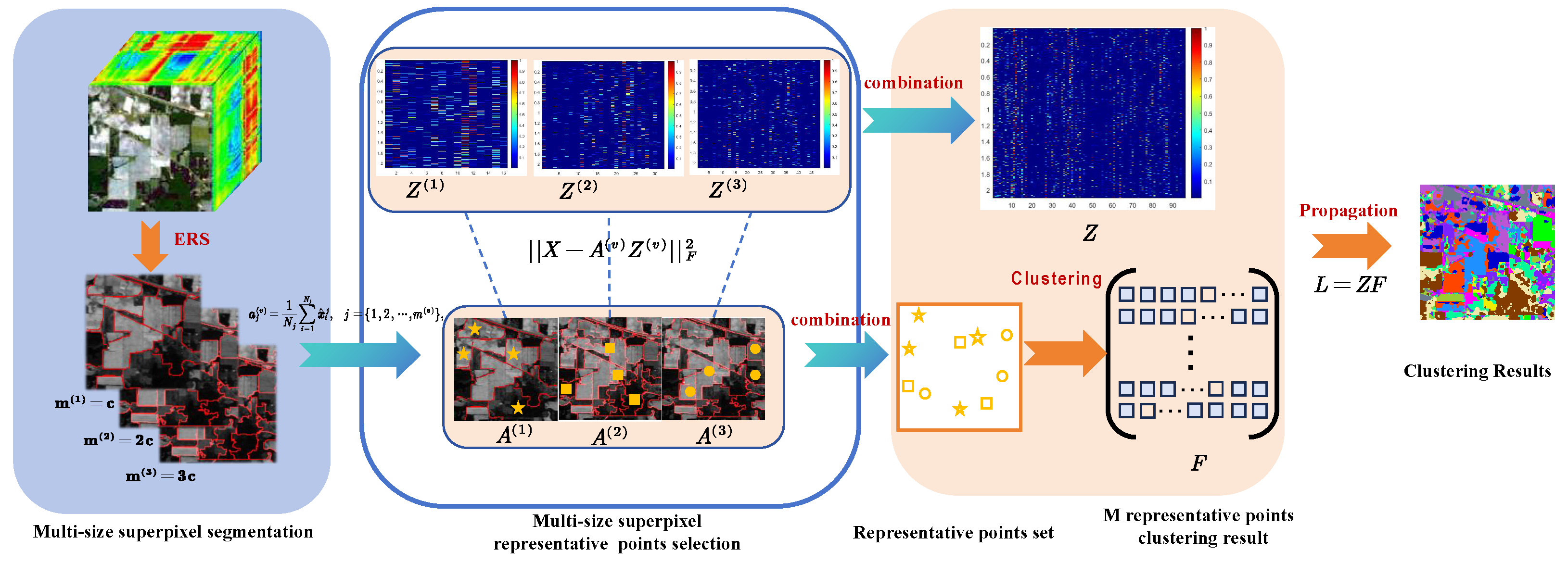
2.1. Adaptive and Diverse Anchor Graph Construction via Multi-Size Superpixel Modeling

To overcome the limitations of fixed anchor configurations in conventional methods, we adopt a flexible anchor graph modeling approach. Specifically, we utilize ERS segmentation to decompose a single hyperspectral image into multiple sets of spatially coherent regions with varying granularities. Each set corresponds to a distinct anchor graph, where the superpixel centroids serve as anchor nodes. By generating multi-size anchor graphs, we effectively capture different levels of structural detail and semantic abstraction.

Notably, our anchor graph construction process is entirely parameter-free. Unlike previous approaches that require manually tuning the number of superpixels or anchors via grid search, our model automatically adapts to the underlying scene complexity without hyperparameter sensitivity. This design not only improves generalizability across different datasets but also ensures robust anchor representation through diverse structural perspectives.

To construct flexible and representative anchor graphs, we employ ERS segmentation to generate multi-scale homogeneous regions from the input hyperspectral image. Each superpixel acts as an anchor node, and the average spectral signature within the superpixel is used as the anchor representation. The entire process is parameter-free and repeated over multiple segmentation granularities to ensure both coarse and fine-scale spatial structure capture.

In image processing, it is widely recognized that pixels belonging to the same class typically form spatially contiguous homogeneous regions, reflecting the inherent structural properties of visual data. Recent advancements in HSI analysis have particularly highlighted the critical role of superpixel segmentation techniques in effectively capturing both the spectral and spatial characteristics of HSI. A comprehensive understanding of HSI data fundamentally relies on the accurate identification of these homogeneous regions, which is essential for subsequent clustering analysis and interpretation. This study employs the ERS method, which, by leveraging pixel spatial distribution and texture features, demonstrates superior performance in generating adaptive homogeneous regions with diverse shapes and scales. Although ERS was originally developed for RGB image segmentation (operating on grayscale-converted single-channel images), its underlying principles make it highly suitable for extension to hyperspectral data. Due to the strong local correlation between adjacent HSI pixels, where neighboring regions often exhibit similar spectral characteristics, integrating this spatial consistency during the preprocessing stage significantly enhances the robustness and accuracy of subsequent clustering tasks. To fully leverage the rich spectral–spatial information in HSI, we adopt a superpixel-based segmentation framework, utilizing the ERS method to maintain spatial coherence while accommodating spectral variability.

As introduced above, we first extract a single representative component from the HSI before performing segmentation. In this work, we employ principal component analysis (PCA) [42] to extract the most informative component. Assume the input HSI is represented as a three-dimensional tensor $\mathcal{X}\in {\mathbb{R}}^{W\times H\times B}$, where $W\times H$ denotes the spatial resolution, and B is the number of spectral bands. We reshape this tensor into a two-dimensional matrix $\mathit{X}\in {\mathbb{R}}^{B\times N}$, where $N=W\times H$. PCA is then applied to $\mathit{X}$ to extract the first principal component, denoted as $I_f$, which captures the majority of the data variance. The ERS algorithm is subsequently applied to $I_f$ to partition the image into M spatially coherent regions, each referred to as a superpixel. This process can be formally expressed as

$$I_f=\bigcup _{i=1}^M{H}_i,\mathrm{s}.\mathrm{t}.H_i\cap H_j=⌀,(i\ne j),$$

(1)

where $H_i$ denotes the i-th homogeneous region corresponding to a superpixel. The non-overlapping constraint $H_i\cap H_j=⌀$ ensures that each pixel is assigned to exactly one region, maintaining disjoint segmentation labels across the image.

Based on the obtained superpixels, we introduce a spatially aware strategy for identifying high-confidence representative pixels. Specifically, each superpixel is characterized by computing the average of all its constituent pixels, which effectively captures both local spectral statistics and spatial consistency. The representative pixel of the j-th superpixel is computed as

$${\mathit{a}}_j={\displaystyle \frac{1}{N_j}}\sum _{i=1}^{N_j}{\hat{\mathit{x}}}_i^j,j=\{1,2,\cdots ,M\},$$

(2)

where ${\widehat{\mathit{x}}}_i^j$ denotes the i-th pixel within the j-th superpixel, and $N_j$ is the total number of pixels in that superpixel. As a result, the total number of image pixels N can be expressed as $N={\sum }_{j=1}^M{N}_j$. Compared with random sampling or K-means-based anchor selection, this strategy ensures that the representative pixels exhibit better spatial coherence and are more aligned with the underlying semantic structures of the image.

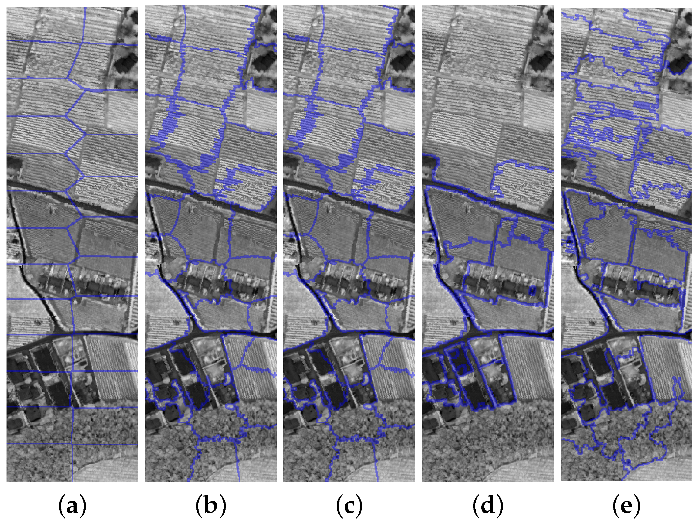
To further enhance spatial adaptability and represent multi-scale contextual information, we design a hierarchical segmentation strategy that operates across multiple spatial resolutions. Specifically, by progressively adjusting the superpixel parameters according to a predefined set, such as $[c,3c,5c,7c,9c]$ where c denotes the estimated number of semantic categories, we generate V distinct segmentation maps, each denoted as ${\mathit{A}}^{\left(v\right)}$. These segmentations represent the scene at varying spatial granularities. Coarse-scale segmentations (e.g., with c superpixels) emphasize global semantic contours, while fine-scale segmentations (e.g., with $9c$ superpixels) preserve detailed local variations.

The integration of these multi-scale representations strengthens the robustness of superpixel-based modeling and lays the foundation for a spatially adaptive clustering framework that can better accommodate heterogeneous land-cover distributions in real-world hyperspectral scenes.

To support the construction of adaptive and diverse anchor graphs, we introduce a hierarchical anchor-pixel association mechanism that aggregates spectral–spatial relationships from multiple ERS segmentations. Rather than working directly on pixel-level data, we leverage representative anchor nodes obtained from superpixels at different granularities and express each pixel as a convex combination of its corresponding anchors. To build a robust and structure-aware anchor graph, we introduce an anchor-pixel association mechanism that derives representative anchor nodes from spatially coherent regions and links them to pixel-level observations across multiple anchor sizes. The process begins by applying ERS segmentation to the hyperspectral image, allowing the extraction of homogeneous regions that preserve local spatial structure.

We perform ERS segmentation on the above $I_f$ using multiple anchor sizes, determined by a predefined set of anchor numbers, such as $[c,3c,5c,7c,9c]$, where c is the estimated number of semantic classes. Each segmentation result yields a set of superpixels, with each superpixel treated as a potential anchor node. For the v-th anchor size, we denote the number of superpixels (i.e., anchors) as $m^{\left(v\right)}$, and each anchor ${\mathit{a}}_j^{\left(v\right)}$ is computed as the mean of its constituent pixel vectors

$${\mathit{a}}_j^{\left(v\right)}={\displaystyle \frac{1}{N_j}}\sum _{i=1}^{N_j}{\widehat{\mathit{x}}}_i^j,j=\{1,2,\cdots ,m^{\left(v\right)}\},$$

(3)

where ${\widehat{\mathit{x}}}_i^j$ is the i-th pixel in the j-th superpixel, and $N_j$ is the number of pixels within that superpixel. This averaging operation ensures spatial coherence and reduces the influence of noise or isolated pixels.

To capture the relationships between anchors and all pixels, we define a non-negative association matrix ${\mathit{Z}}^{\left(v\right)}\in {\mathbb{R}}^{m^{\left(v\right)}\times N}$ for each anchor size. Each column in ${\mathit{Z}}^{\left(v\right)}$ corresponds to a pixel and encodes its similarity or membership to all anchors at that size. To ensure interpretability and probabilistic meaning, we constrain the memberships to be non-negative and sum to one

$$\underset{{\mathit{Z}}^{\left(v\right)}}{min}{\Vert \mathit{X}-{\mathit{A}}^{\left(v\right)}{\mathit{Z}}^{\left(v\right)}\Vert }_F^2,\mathrm{s}.\mathrm{t}.{\mathit{Z}}^{\left(v\right)T}\mathbf{1}=\mathbf{1},{\mathit{Z}}^{\left(v\right)}\ge 0,$$

(4)

where ${\mathit{A}}^{\left(v\right)}=[{\mathit{a}}_1^{\left(v\right)},\dots ,{\mathit{a}}_{m^{\left(v\right)}}^{\left(v\right)}]\in {\mathbb{R}}^{B\times m^{\left(v\right)}}$ is the anchor matrix at the v-scale.

Finally, we concatenate all ${\mathit{Z}}^{\left(v\right)}$ across V anchor sizes to form a unified anchor-pixel association matrix

$$\mathit{Z}=\left[{\mathit{Z}}^{\left(1\right)};{\mathit{Z}}^{\left(2\right)};\dots ;{\mathit{Z}}^{\left(V\right)}\right]\in {\mathbb{R}}^{M\times N},M=\sum _{v=1}^V{m}^{\left(v\right)}.$$

(5)

This unified representation enables the framework to integrate coarse-to-fine spatial structure through diverse anchor sizes and supports adaptive representation of heterogeneous land-cover patterns. The resulting $\mathit{Z}$ serves as the foundation for subsequent graph construction and anchor-level clustering.

2.2. Anchor-Level Graph Clustering via Laplacian Rank Optimization

With the unified anchor-pixel association matrix $\mathit{Z}$ serving as the low-dimensional representation of hyperspectral data, we perform clustering directly on anchor nodes to reduce computational overhead and enhance structural abstraction. To capture the underlying semantic relationships between these representative anchors, we construct an optimized similarity graph $\mathit{S}$, which reflects both geometric proximity and global semantic consistency.

In our framework, the anchors derived from each scale are independently extracted from the original hyperspectral data using superpixel segmentation, resulting in anchor matrices ${\mathit{A}}^{\left(v\right)}\in {\mathbb{R}}^{B\times m^{\left(v\right)}}$, where v denotes the scale index and $m^{\left(v\right)}$ is the number of anchors at scale v. Each scale’s anchors reside in the same spectral feature space, ${\mathbb{R}}^B$, and are thus naturally aligned at the feature level. To fully exploit the complementary information across different scales, we concatenate these anchors along the feature dimension as follows:

$$\mathit{A}=[{\mathit{A}}^{\left(1\right)},{\mathit{A}}^{\left(2\right)},\dots ,{\mathit{A}}^{\left(V\right)}]\in {\mathbb{R}}^{B\times M},$$

(6)

where $M={\sum }_{v=1}^V{m}^{\left(v\right)}$ is the total number of anchors. Since all anchors reside in the same spectral feature space ${\mathbb{R}}^B$, they are naturally aligned at the feature level. This direct concatenation enables the fused anchor set to preserve scale-specific spatial semantics while ensuring spectral consistency, thereby eliminating the need for explicit spatial or feature alignment. This matrix serves as the clustering input, transforming the original pixel space into a more compact and spatially coherent representation. By concatenating anchors from different scales, we preserve their scale-specific spatial semantics while ensuring spectral consistency.

To learn the similarity matrix $\mathit{S}$, we formulate the following optimization problem:

$$\underset{\mathit{S}}{min}\sum _{i=1}^M\sum _{j=1}^M\parallel {\mathit{a}}_i-{\mathit{a}}_j{\parallel }_2^2{s}_{ij}+\lambda {\parallel \mathit{S}\parallel }_F^2,\mathrm{s}.\mathrm{t}.\mathit{S}\mathbf{1}=\mathbf{1},\mathit{S}\ge 0,\mathrm{rank}\left({\mathit{L}}_S\right)=M-c.$$

(7)

Here, $s_{ij}$ denotes the similarity between anchors ${\mathit{a}}_i$ and ${\mathit{a}}_j$, promoting stronger connections for spectrally similar regions. The regularization term ${\parallel \mathit{S}\parallel }_F^2$ encourages sparsity and smoothness, while the row-stochastic constraint ensures probabilistic interpretation. The Laplacian matrix ${\mathit{L}}_S$ is defined as

$${\mathit{L}}_S={\mathit{D}}_S-{\displaystyle \frac{1}{2}}(\mathit{S}+{\mathit{S}}^T),$$

(8)

where the degree matrix ${\mathit{D}}_S$ is computed via $\mathrm{diag}\left({\sum }_j{\displaystyle \frac{s_{ij}+s_{ji}}{2}}\right)$.

Crucially, we enforce a rank constraint $\mathrm{rank}\left({\mathit{L}}_S\right)=M-c$, which guarantees that the similarity graph contains exactly c connected components—each corresponding to a distinct semantic cluster in the hyperspectral image.

Theorem 1. 

The multiplicity of the zero eigenvalue of the Laplacian matrix ${\mathit{L}}_S$ equals the number of connected components in the graph defined by $\mathit{S}$.

This spectral graph-theoretic result ensures that minimizing the Laplacian rank directly yields a semantically consistent partition of the anchors, eliminating the need for additional post-processing such as K-means. The final clustering assignment is thus derived in a fully unsupervised and structure-preserving manner, leveraging anchor-level abstraction for efficient and robust hyperspectral image segmentation.

2.3. Anchor-to-Pixel Label Propagation

To effectively transfer semantic information from the representative anchors to the full set of pixels, we apply a label propagation mechanism based on the learned soft association matrix between anchors and pixels. This approach allows the rich semantic cues captured at the anchor level to be diffused throughout the image, providing dense pixel-level predictions. By doing so, the method not only preserves the spectral characteristics of the data but also enforces spatial coherence, ensuring that neighboring pixels with similar features receive consistent labels. This propagation step is crucial for bridging the gap between the sparse anchor representations and the detailed pixel-wise segmentation, ultimately improving the accuracy and robustness of the clustering results.

3. Optimization and Anchor-to-Pixel Label Propagation

This section presents the optimization strategy of our proposed framework and the final semantic diffusion step. The optimization proceeds in two stages: (1) learning the adaptive anchor-pixel association through constrained reconstruction and (2) discovering semantically coherent anchor groups by graph optimization. The final clustering output is then propagated from anchor nodes to pixels to obtain spatially continuous and semantically interpretable segmentation.

3.1. Anchor-Pixel Association via Quadratic Programming

Given the input data matrix $\mathit{X}\in {\mathbb{R}}^{B\times N}$ and the representative anchor sets ${\left\{{\mathit{A}}^{\left(v\right)}\right\}}_{v=1}^V$ constructed from ERS segmentations of various sizes, we optimize the anchor-pixel association matrices ${\mathit{Z}}^{\left(v\right)}\in {\mathbb{R}}^{m^{\left(v\right)}\times N}$ by minimizing the following objective:

$$\begin{array}{c}\underset{{\mathit{Z}}^{\left(v\right)}}{min}\sum _{v=1}^V{\parallel \mathit{X}-{\mathit{A}}^{\left(v\right)}{\mathit{Z}}^{\left(v\right)}\parallel }_F^2,\mathrm{s}.\mathrm{t}.{\mathit{Z}}^{\left(v\right)T}\mathbf{1}=\mathbf{1},{\mathit{Z}}^{\left(v\right)}\ge 0.\end{array}$$

(9)

This problem decomposes over individual pixels, resulting in a set of n constrained QP subproblems of the form:

$$\begin{array}{c}\underset{{\mathit{z}}_i^{\left(v\right)}}{min}{\parallel {\mathit{x}}_i-{\mathit{A}}^{\left(v\right)}{\mathit{z}}_i^{\left(v\right)}\parallel }_2^2,\mathrm{s}.\mathrm{t}.{\mathit{z}}_i^{\left(v\right)T}\mathbf{1}=1,{\mathit{z}}_i^{\left(v\right)}\ge 0.\end{array}$$

(10)

We solve these using standard QP solvers. Once solved, the concatenated form

$$\mathit{Z}=[{\mathit{Z}}^{\left(1\right)};{\mathit{Z}}^{\left(2\right)};\dots ;{\mathit{Z}}^{\left(V\right)}]\in {\mathbb{R}}^{M\times N}$$

(11)

serves as a unified low-dimensional embedding that bridges anchors and pixels across different sizes.

3.2. Graph-Based Anchor Clustering via Laplacian Rank Minimization

To cluster the anchors efficiently, we optimize the similarity matrix $\mathit{S}$ among all m anchors by solving the following graph-based learning problem:

$$\begin{array}{c}\begin{array}{ccc}\hfill & \underset{\mathit{S}}{min}\sum _{i,j=1}^M{\parallel {\mathit{a}}_i-{\mathit{a}}_j\parallel }_2^2{\mathit{s}}_{ij}+\lambda {\parallel \mathit{S}\parallel }_F^2,\hfill & \hfill \mathrm{s}.\mathrm{t}.\mathit{S}\mathbf{1}=\mathbf{1},\mathit{S}\ge 0,\mathrm{rank}\left({\mathit{L}}_S\right)=M-c.\end{array}\end{array}$$

(12)

This formulation ensures that the resulting Laplacian matrix ${\mathit{L}}_S$ leads to exactly c connected components, i.e., c clusters. It can be seen that the Equation (12) is equivalent to the following problem for a large enough value of $\gamma$:

$$\begin{array}{cc}\underset{\mathit{S}}{min}\sum _{i=1}^M\sum _{j=1}^M{\parallel {\mathit{a}}_i-{\mathit{a}}_j\parallel }_2^2{\mathit{s}}_{ij}+\lambda {\parallel \mathit{S}\parallel }_F^2+2\gamma \sum _{i=1}^c{\sigma }_i\left({\mathit{L}}_S\right)\hfill & \hfill \mathrm{s}.\mathrm{t}.\mathit{S}\mathbf{1}=\mathbf{1},\mathit{S}⪰0.\end{array}$$

(13)

It can be further relaxed via the Ky Fan [43] theorem into a jointly optimized trace form. We can apply the alternative optimization approach to solve it.

$$\begin{array}{c}\underset{\mathit{S},\mathit{F}}{min}\sum _{i,j=1}^M\left({\parallel {\mathit{a}}_i-{\mathit{a}}_j\parallel }_2^2{s}_{ij}+\lambda s_{ij}^2\right)+2\gamma Tr\left({\mathit{F}}^{\top }{\mathit{L}}_S\mathit{F}\right)\hfill \\ \mathrm{s}.\mathrm{t}.\forall i,{\mathit{s}}_i^{\top }\mathbf{1}=1,0\le s_{ij}\le 1,\mathit{F}\in {\mathbb{R}}^{M\times c},{\mathit{F}}^{\top }\mathit{F}=\mathit{I}.\hfill \end{array}$$

(14)

When $\mathit{S}$ is fixed, the Equation (14) becomes

$$\begin{array}{c}\hfill \underset{\begin{array}{c}\mathit{F}\in {\mathbb{R}}^{M\times c},{\mathit{F}}^T\mathit{F}=\mathit{I}\end{array}}{min}Tr\left({\mathit{F}}^T{\mathit{L}}_S\mathit{F}\right).\end{array}$$

(15)

The optimal solution $\mathit{F}$ to Equation (15) is formed by the c eigenvectors of ${\mathit{L}}_S$ corresponding to the c smallest eigenvalues.

When $\mathit{F}$ is fixed, Equation (14) becomes

$$\begin{array}{ccc}\hfill \underset{\mathit{S}}{min}& \sum _{i,j=1}^M\left({\parallel {\mathit{a}}_i-{\mathit{a}}_j\parallel }_2^2{\mathit{s}}_{ij}+\lambda {\mathit{s}}_{ij}^2\right)+2\gamma \mathrm{Tr}\left({\mathit{F}}^T{\mathit{L}}_S\mathit{F}\right)\hfill & \hfill \mathrm{s}.\mathrm{t}.\forall i,{\mathit{s}}_i^T\mathbf{1}=1,0\le {\mathit{s}}_i\le 1.\end{array}$$

(16)

According to ${\sum }_{i,j=1}^N{\parallel f_i-f_j\parallel }_2^2{s}_{ij}=2\mathrm{Tr}\left(F^T{\mathit{L}}_{S}F\right)$, Equation (16) can be rewritten as

$$\begin{array}{ccc}\hfill \underset{\mathit{S}}{min}& \sum _{i,j=1}^M\left({\parallel {\mathit{a}}_i-{\mathit{a}}_j\parallel }_2^2{\mathit{s}}_{ij}+\lambda {\mathit{s}}_{ij}^2+\gamma {\parallel {\mathit{f}}_i-{\mathit{f}}_j\parallel }_2^2{\mathit{s}}_{ij}\right)\hfill & \hfill \mathrm{s}.\mathrm{t}.\forall i,{\mathit{s}}_i^T\mathbf{1}=1,0\le {\mathit{s}}_i\le 1.\end{array}$$

(17)

Note that Equation (17) is independent between different i, so we can solve the following problem individually for each i:

$$\begin{array}{ccc}\hfill \underset{{\mathit{s}}_i}{min}& \sum _{j=1}^M\left(\parallel {\mathit{a}}_i-{\mathit{a}}_j{\parallel }_2^2{\mathit{s}}_{ij}+\lambda {\mathit{s}}_{ij}^2+\gamma {\parallel {\mathit{f}}_i-{\mathit{f}}_j\parallel }_2^2{\mathit{s}}_{ij}\right)\hfill & \hfill \mathrm{s}.\mathrm{t}.{\mathit{s}}_i^T\mathbf{1}=1,0\le {\mathit{s}}_i\le 1.\end{array}$$

(18)

Denote ${\mathit{d}}_{ij}^x={\parallel {\mathit{a}}_i-{\mathit{a}}_j\parallel }_2^2$ and $d_{ij}^f={\parallel {\mathit{f}}_i-{\mathit{f}}_j\parallel }_2^2$, and let ${\mathit{d}}_i\in {\mathbb{R}}^{M\times 1}$ be a vector with the j-th element as ${\mathit{d}}_{ij}={\mathit{d}}_{ij}^x+\lambda {\mathit{d}}_{ij}^f$. To accelerate the procedure, $\lambda$ can be determined during the iteration. We can initialize $\lambda =\gamma$ and then increase $\lambda$ if the connected components of $\mathit{S}$ is smaller than c and decrease $\lambda$ if it is greater than c in each iteration. Then, Equation (18) can be written in vector form as

$$\begin{array}{c}\hfill \underset{{\mathit{s}}_i^T\mathbf{1}=1,0\le {\mathit{s}}_i\le 1}{min}{∥{\mathit{s}}_i+{\displaystyle \frac{1}{2\gamma }}{\mathit{d}}_i∥}_2^2.\end{array}$$

(19)

This problem can be solved with a closed form solution. This yields the final anchor-level cluster assignment matrix $\mathit{F}\in {\mathbb{R}}^{M\times c}$.

3.3. Anchor-to-Pixel Semantic Label Propagation

To obtain pixel-level predictions, we diffuse the anchor-level semantic labels back to the original data via the learned membership matrix $\mathit{Z}$. Specifically, we compute

$$\mathit{Y}={\mathit{Z}}^T\mathit{F}\in {\mathbb{R}}^{N\times c},$$

(20)

where ${\mathit{Y}}_{ij}$ represents the confidence that pixel i belongs to class j. The final pixel label is obtained by selecting the index of the maximum value along each row of $\mathit{Y}$. This diffusion step propagates structure-aware semantic labels to the pixel domain, ensuring that the segmentation is not only spectrally consistent but also spatially coherent. The abel propagation is showed in Figure 2.

3.4. Computational Complexity Analysis

This section analyzes the overall computational complexity of the proposed method, which consists of three key stages: adaptive anchor graph construction via multi-scale superpixel modeling, anchor clustering under Laplacian rank constraints, and anchor-to-pixel label propagation.

In the anchor graph construction stage, the complexity of computing the anchor-pixel association matrix is $\mathcal{O}(N\ast M\ast m_{avg})$, where $M={\sum }_{v=1}^V{m}^{\left(v\right)}$ denotes the total number of anchors across all scales, and $m_{\mathrm{avg}}$ is the average number of anchors per scale. Since the number of anchors $m^{\left(v\right)}$ is typically much smaller than the number of pixels N, this step is computationally efficient, especially when the number of anchors is small.

In the anchor clustering stage, the algorithm alternates between two steps, updating the feature matrix $\mathbf{F}$ via eigen-decomposition of the Laplacian matrix and updating the similarity matrix $\mathbf{S}$ row by row. The complexity of updating $\mathbf{F}$ is $\mathcal{O}(M^2\ast c)$, while the complexity of updating $\mathbf{S}$ is $\mathcal{O}(M^2\ast (B+c))$, where B is the input feature dimension. Assuming the algorithm converges in T iterations, the total complexity of this stage is $\mathcal{O}(T\ast M^2\ast (B+c))$.

In the label propagation stage, semantic labels are transferred from anchors to pixels via matrix multiplication, with a complexity of $\mathcal{O}(N\ast M\ast c)$. Given that both M and c are typically much smaller than N, this step is also computationally efficient. In summary, the overall time complexity of the proposed method is $\mathcal{O}\left(N\ast M\ast m_{\mathrm{avg}}+N\ast M\ast c\right)$. This complexity is scalable and well suited for large-scale hyperspectral image clustering tasks.

4. Experiments

4.1. Datasets

To evaluate the effectiveness and generalizability of the proposed method, experiments are conducted on three widely used public HSI datasets: Trento, Salinas, and Pavia Center. These datasets vary in spatial resolution, number of spectral bands, land-cover complexity, and acquisition sensors, providing a comprehensive benchmark for HSI clustering tasks.

(1) Trento: The Trento dataset was acquired over a rural area south of Trento, Italy, and includes both hyperspectral and LiDAR modalities. The spatial size of the image is $600\times 166$ pixels with a spatial resolution of 1 m. The hyperspectral data were collected using the AISA Eagle sensor, covering 63 spectral bands in the wavelength range of 0.40 to 0.98 μm. Additionally, the LiDAR data were obtained using the Optech ALTM 3100EA system (Teledyne Optech, Vaughan, ON, Canada) and contain two elevation-based channels. A total of six land-cover classes are annotated in the scene, including buildings, roads, trees, and bare soil, among others.

(2) Salinas: This dataset was collected over the Salinas Valley, California, using the AVIRIS airborne sensor (Jet Propulsion Laboratory, Pasadena, CA, USA) in 1998. The hyperspectral cube consists of $512\times 217$ pixels and originally contains 224 spectral bands with a spatial resolution of 3.7 m. After removing 20 water absorption bands (i.e., bands 108–112, 154–167, and 224), a total of 204 spectral bands are retained for analysis. The dataset comprises 111,104 labeled pixels distributed across 16 distinct vegetation and soil-related classes, making it one of the most challenging and high-resolution HSI datasets available.

(3) Pavia Center: The Pavia Center dataset was acquired by the Reflective Optics System Imaging Spectrometer sensor (DLR-German Aerospace Center, Wessling, Germany) over an urban area in Pavia, northern Italy. The original image has a spatial dimension of $1096\times 1096$ pixels and includes 102 spectral bands after discarding noisy bands. Due to background noise and non-informative regions, only the central portion of the image ($1096\times 715$ pixels) is used for experiments. In total, the dataset contains 783,640 labeled pixels across nine urban scene categories such as asphalt, meadows, and buildings.

4.2. Compared Methods

To comprehensively validate the clustering performance of our proposed method, we compare it against eight state-of-the-art and representative clustering algorithms from the literature. These methods span a variety of modeling paradigms including spectral–spatial fusion, graph-based learning, fuzzy clustering, and sparse subspace modeling. The following algorithms are selected for comparison:

• ACLR [44]—Adaptive Collaborative Low-Rank clustering.
• EDCAG [45]—Enhanced Deep Clustering via Affinity Graph learning.
• FCM [46]—Classical Fuzzy C-Means algorithm.
• FSC [47]—Fuzzy Subspace Clustering with feature selection.
• SGCNR [48]—Spectral Graph Constrained Nonnegative Representation.
• FCAG [49]—Fuzzy Clustering with Adaptive Graph learning.
• USPEC [50]—Ultra-Scalable Spectral Clustering for large-scale HSI data.
• FSSC [51]—Fast Sparse Subspace Clustering.

For fair comparison, all methods are tuned using their optimal or recommended parameter settings as reported in the respective literature. Where applicable, we follow the authors’ publicly available implementations or reimplement the methods under the same experimental conditions.

4.3. Experimental Settings

To quantitatively assess the clustering performance, we adopt four commonly used evaluation metrics in the hyperspectral analysis community: Overall Accuracy (OA), Average Accuracy (AA), User’s Accuracy (UA), and the Kappa Coefficient (Kappa). Their definitions and significance are summarized as follows:

• Overall Accuracy (OA): Measures the proportion of correctly clustered pixels across the entire dataset. It reflects the global performance of the clustering model.
• Average Accuracy (AA): Computes the mean of per-class accuracies, offering a balanced assessment that accounts for class imbalance.
• User’s Accuracy (UA): Indicates the accuracy with which each class is clustered, providing class-specific insight into model performance.
• Kappa Coefficient (Kappa): A statistical measure that quantifies the agreement between predicted and ground-truth clustering, normalized by chance agreement. It is particularly robust in imbalanced settings.

All metrics are computed by aligning the unsupervised clustering labels with the ground truth through the Hungarian algorithm to ensure fair evaluation. Higher values for all metrics indicate superior clustering performance. Each experiment is independently repeated five times, and the average results are reported to mitigate the effects of random initialization.

To ensure fairness and reproducibility across all experiments, we adopt fixed hyperparameter settings [c, 3c, 5c, 7c, 9c] for our model. Specifically, a multi-granularity anchor extraction strategy is employed. We perform superpixel segmentation at five different levels of granularity: where c denotes the base superpixel size, empirically determined based on the resolution of each dataset and the scale of typical objects. Coarse granularity (e.g., 9c) is used to represent large and homogeneous regions, while fine granularity (e.g., c) is better suited to capture detailed structures and fragmented areas. This multi-scale strategy enables the model to comprehensively represent both broad-scale and fine-grained spatial structures, thereby improving the generalizability and robustness of the proposed method. For the hyperparameters of comparative methods, we strictly follow the values specified in the experimental sections of their respective papers to ensure fairness and validity in comparisons.

Regarding the choice of anchor sizes, we first designed multiple parameter combinations within the range of [c, 10c] and conducted systematic comparative experiments on several benchmark datasets to comprehensively evaluate the impact of different configurations on clustering performance.

The experimental results indicate that our method consistently achieves stable and excellent clustering performance under various parameter settings. This demonstrates the robustness and adaptability of our approach to different scale configurations. Among all tested combinations, the multi-scale anchor sizes of [c, 3c, 5c, 7c, 9c] stand out. This combination achieves a good balance between fine-grained and coarse-grained feature representation, delivering the most stable and competitive results, reflecting strong generalization ability.

Furthermore, this configuration not only suits diverse scenarios and object distributions but also avoids the need for manual tuning of anchor numbers for each dataset, highlighting the parameter-free design and adaptability of our method.

To present these findings more intuitively,

Table 2. Clustering performance under different superpixel group combinations across datasets. (The Best Value in Each Column is in Bold).

Dataset	Superpixel Group	AA (%)	OA (%)	Kappa
Salinas	[2c, 4c, 6c, 8c]	57.94	62.08	0.5766
	[2c, 4c, 6c, 8c, 10c]	65.12	68.61	0.6505
	[1c, 3c, 5c, 7c]	59.61	69.97	0.6591
	[1c, 3c, 5c]	53.15	61.84	0.5669
	[1c, 3c, 5c, 7c, 9c]	60.18	71.87	0.6842
Trento	[2c, 4c, 6c, 8c]	62.56	80.19	0.7284
	[2c, 4c, 6c, 8c, 10c]	67.01	80.89	0.7243
	[1c, 3c, 5c, 7c]	63.20	75.38	0.6780
	[1c, 3c, 5c]	56.26	71.22	0.6236
	[1c, 3c, 5c, 7c, 9c]	66.21	81.10	0.7494
Pavia_centre	[2c, 4c, 6c, 8c]	50.28	75.04	0.6502
	[2c, 4c, 6c, 8c, 10c]	53.71	77.21	0.6771
	[1c, 3c, 5c, 7c]	47.34	75.26	0.6539
	[1c, 3c, 5c]	44.03	82.25	0.7107
	[1c, 3c, 5c, 7c, 9c]	44.85	83.36	0.7495

summarizes the clustering performance of different superpixel combinations across multiple datasets. Although this combination does not yield the highest AA score on the Pavia Center dataset, it outperforms others on all other key metrics across the three datasets, further validating its overall robustness and superiority. In summary, the multi-scale combination [1c, 3c, 5c, 7c, 9c] is chosen as the default parameter setting in our main experiments due to its stability and general applicability.

5. Results

The evaluation results of various methods are summarized in Table 3, Table 4 and Table 5, with the optimal values highlighted in bold. Based on these results, we have the following observations:

5.1. Experimental Results on the Trento Dataset

Table 3 reports the clustering performance of our method compared with eight state-of-the-art baselines on the Trento hyperspectral dataset. The evaluation includes class-wise UA, OA, AA, and the Kappa coefficient. Our method achieves an OA of 81.10% and a Kappa of 0.7494, consistently outperforming all baselines. This demonstrates the effectiveness of our unsupervised framework in capturing complex spectral–spatial structures under real-world rural conditions. The results presented in Figure 3 demonstrate superior performance in maintaining regional consistency and minimizing misclassified pixels, providing compelling visual evidence of the method’s effectiveness.

Table 3. Experimental clustering results of compared approaches in the Trento dataset. (The Best Value in Each Row is in Bold).

Class	ACLR	EDCAG	FCM	FSC	SGCNR	FCAG	USPEC	FSSC	OURS
Apple trees	28.48	63.58	72.70	87.67	81.08	76.72	67.50	94.59	81.13
Corn-notill	77.07	0.00	97.76	74.40	82.01	98.58	99.93	94.41	80.70
Buildings	0.00	1.25	68.26	0.00	2.71	0.00	1.04	0.00	0.00
Ground	93.45	55.04	66.78	44.41	42.69	43.60	47.15	42.57	73.93
Vineyard	91.06	32.53	49.17	52.09	54.91	37.10	54.95	61.10	95.76
Wood	68.32	94.73	13.23	69.18	58.31	18.08	5.45	16.25	65.72
AA(%)	55.00	63.37	66.87	61.32	55.96	71.62	51.63	51.69	66.21
OA(%)	58.75	59.65	59.96	58.83	59.66	61.76	54.87	57.62	81.10
Kappa	0.4876	0.4848	0.4947	0.4778	0.4972	0.5173	0.4500	0.4706	0.7494

Table 3. Experimental clustering results of compared approaches in the Trento dataset. (The Best Value in Each Row is in Bold).

Class	ACLR	EDCAG	FCM	FSC	SGCNR	FCAG	USPEC	FSSC	OURS
Apple trees	28.48	63.58	72.70	87.67	81.08	76.72	67.50	94.59	81.13
Corn-notill	77.07	0.00	97.76	74.40	82.01	98.58	99.93	94.41	80.70
Buildings	0.00	1.25	68.26	0.00	2.71	0.00	1.04	0.00	0.00
Ground	93.45	55.04	66.78	44.41	42.69	43.60	47.15	42.57	73.93
Vineyard	91.06	32.53	49.17	52.09	54.91	37.10	54.95	61.10	95.76
Wood	68.32	94.73	13.23	69.18	58.31	18.08	5.45	16.25	65.72
AA(%)	55.00	63.37	66.87	61.32	55.96	71.62	51.63	51.69	66.21
OA(%)	58.75	59.65	59.96	58.83	59.66	61.76	54.87	57.62	81.10
Kappa	0.4876	0.4848	0.4947	0.4778	0.4972	0.5173	0.4500	0.4706	0.7494

The superior performance stems from the seamless integration of our three core contributions. First, the anchor graph construction is entirely data-driven and multi-size in nature. By generating multiple anchor graphs from entropy-rate superpixels of varying sizes, our framework adaptively captures spatial patterns at different structural granularities without requiring any manual parameter tuning. This proves especially beneficial for classes with subtle spatial boundaries or nested structures, such as “Vineyard” and “Apple trees,” where we obtain class-wise accuracies of 95.76% and 81.13%, respectively.

Second, our adaptive anchor-pixel association ensures robust and flexible representation learning. The use of constrained soft membership optimization allows each pixel to be reconstructed by a convex combination of multiple anchors, enabling the model to gracefully handle mixed pixels and ambiguous regions. This adaptive mechanism significantly improves clustering stability and generalization, particularly for the “Ground” category—known for its high spectral variability—where we achieve 73.93% accuracy, surpassing most fixed-assignment baselines.

Finally, the semantic clustering is performed efficiently on the anchor level through graph-based optimization, where we enforce rank constraints on the Laplacian to yield semantically meaningful clusters. The anchor-to-pixel label propagation step diffuses these high-level decisions to the entire image in a structure-aware manner. This two-stage design enhances spatial coherence and reduces random noise, leading to consistent and interpretable cluster maps, as evidenced by the highest Kappa score among all methods.

In contrast to baselines that often excel in specific categories but struggle with generalization, our method achieves balanced performance across all land-cover types, showcasing strong robustness and discriminative power under fully unsupervised conditions.

5.2. Experimental Results on the Salinas Dataset

Table 4 summarizes the clustering results of our method and multiple baselines on the Salinas dataset. Our method achieves the best OA of 71.87% and the highest Kappa coefficient of 0.6842, demonstrating a significant improvement over existing methods. Although the AA is slightly lower than that of SGCNR, our approach consistently delivers competitive performance across nearly all classes, reflecting its robustness under complex agricultural settings. As can be seen from Figure 4, it demonstrates outstanding performance in terms of regional uniformity and misclassified pixels, further proving its effectiveness.

Table 4. Experimental clustering results of compared approaches in the Salinas dataset. (The Best Value in Each Row is in Bold).

Class	ACLR	EDCAG	FCM	FSC	SGCNR	FCAG	USPEC	FSSC	OURS
Weeds_1	99.74	0.00	99.70	97.81	95.07	73.07	0.00	76.56	0.00
Weeds_2	97.71	95.35	39.88	94.82	97.99	61.43	98.65	92.49	98.98
Fallow	0.00	53.69	0.00	65.33	74.29	23.43	42.86	0.00	0.00
Fallow_plow	96.46	97.56	96.56	72.96	99.57	99.85	99.71	0.00	99.78
Fallow_smooth	70.09	83.60	95.74	92.87	85.10	49.73	91.85	93.95	92.94
Stubble	100.00	92.57	82.78	93.63	97.88	81.63	99.39	99.24	99.97
Celery	98.04	98.54	94.10	54.46	99.39	96.81	99.41	98.85	99.94
Grapes_untrained	96.80	42.56	42.56	60.40	61.27	48.71	98.22	98.43	81.70
Soil	73.66	81.81	99.24	88.89	97.73	64.33	64.22	99.95	87.42
Corn	47.17	40.48	0.24	4.18	65.59	62.90	4.24	0.06	70.98
Lettuce_4wk	82.60	3.83	7.24	37.36	14.23	46.06	84.17	0.00	0.00
Lettuce_5wk	0.00	48.72	98.50	98.55	34.46	0.00	82.04	0.00	70.78
Lettuce_6wk	88.95	97.48	98.69	0.00	98.58	97.16	98.03	0.00	0.00
Lettuce_7wk	90.73	89.81	88.79	96.64	89.63	95.42	89.25	90.19	99.71
Vinyard_untrained	0.00	0.16	58.53	64.53	62.71	46.29	0.00	0.02	60.63
Vinyard_trellis	39.21	0.00	43.22	74.99	0.00	71.16	0.00	45.49	0.00
AA (%)	65.72	62.70	65.37	65.58	66.17	63.62	65.75	49.71	60.18
OA (%)	69.24	67.56	62.58	69.80	70.79	59.55	65.38	62.93	71.87
Kappa	0.6508	0.6369	0.5876	0.6639	0.6785	0.5566	0.6091	0.5746	0.6842

Table 4. Experimental clustering results of compared approaches in the Salinas dataset. (The Best Value in Each Row is in Bold).

Class	ACLR	EDCAG	FCM	FSC	SGCNR	FCAG	USPEC	FSSC	OURS
Weeds_1	99.74	0.00	99.70	97.81	95.07	73.07	0.00	76.56	0.00
Weeds_2	97.71	95.35	39.88	94.82	97.99	61.43	98.65	92.49	98.98
Fallow	0.00	53.69	0.00	65.33	74.29	23.43	42.86	0.00	0.00
Fallow_plow	96.46	97.56	96.56	72.96	99.57	99.85	99.71	0.00	99.78
Fallow_smooth	70.09	83.60	95.74	92.87	85.10	49.73	91.85	93.95	92.94
Stubble	100.00	92.57	82.78	93.63	97.88	81.63	99.39	99.24	99.97
Celery	98.04	98.54	94.10	54.46	99.39	96.81	99.41	98.85	99.94
Grapes_untrained	96.80	42.56	42.56	60.40	61.27	48.71	98.22	98.43	81.70
Soil	73.66	81.81	99.24	88.89	97.73	64.33	64.22	99.95	87.42
Corn	47.17	40.48	0.24	4.18	65.59	62.90	4.24	0.06	70.98
Lettuce_4wk	82.60	3.83	7.24	37.36	14.23	46.06	84.17	0.00	0.00
Lettuce_5wk	0.00	48.72	98.50	98.55	34.46	0.00	82.04	0.00	70.78
Lettuce_6wk	88.95	97.48	98.69	0.00	98.58	97.16	98.03	0.00	0.00
Lettuce_7wk	90.73	89.81	88.79	96.64	89.63	95.42	89.25	90.19	99.71
Vinyard_untrained	0.00	0.16	58.53	64.53	62.71	46.29	0.00	0.02	60.63
Vinyard_trellis	39.21	0.00	43.22	74.99	0.00	71.16	0.00	45.49	0.00
AA (%)	65.72	62.70	65.37	65.58	66.17	63.62	65.75	49.71	60.18
OA (%)	69.24	67.56	62.58	69.80	70.79	59.55	65.38	62.93	71.87
Kappa	0.6508	0.6369	0.5876	0.6639	0.6785	0.5566	0.6091	0.5746	0.6842

The Salinas scene is particularly challenging due to its high number of land-cover classes (16), subtle spectral distinctions among similar crop types, and notable intra-class variability. These challenges emphasize the necessity of our three-fold design.

First, our parameter-free construction of adaptive and diverse anchor graphs allows the model to flexibly represent spatial structures at different granularities. By leveraging entropy rate-based superpixels of varying sizes, the framework captures both large-scale field patterns and fine-grained vegetation patches. For example, the model achieves high accuracy on structurally consistent classes such as “Fallow_plow” (99.78%) and “Celery” (99.94%), benefiting from its ability to encode multiscale spatial context without manual tuning.

Second, by shifting clustering from the pixel level to the anchor level, we significantly reduce computational complexity while preserving the discriminative structure of the image. Anchors—defined as superpixel-level representatives—act as compact surrogates for their associated regions, capturing local spectral statistics and enhancing semantic coherence. This leads to improved robustness against noise and outliers, as demonstrated in spectrally ambiguous categories like “Corn” (70.98%) and “Stubble” (99.97%).

Third, our anchor-to-pixel label propagation mechanism bridges the abstract anchor clustering results back to pixel-level interpretations. Through a graph-optimized process with rank-constrained Laplacian learning, the framework ensures that final pixel assignments reflect both the global semantic structure and local spatial continuity. This is particularly evident in the “Lettuce_7wk” class (99.71%), where the method maintains high accuracy despite heterogeneous texture and boundary complexity.

While some baselines exhibit strong performance on isolated classes (e.g., FCM on “Fallow_smooth”), they often lack generalization across the entire scene. In contrast, our method delivers balanced, scene-level clustering performance across both dominant and difficult classes. These results affirm the effectiveness of integrating adaptive spatial priors, anchor-level abstraction, and structure-aware propagation for robust unsupervised hyperspectral image clustering.

5.3. Experimental Results on the Pavia Center Dataset

Table 5 reports the clustering performance on the Pavia Center dataset. Figure 5 illustrates how the proposed technique preserves structural uniformity while reducing classification errors—key advantages over conventional methods. Our method achieves the highest OA of 83.36% and the best Kappa coefficient of 0.7495, consistently outperforming all baselines. This urban scene poses substantial challenges due to small-scale man-made structures, intricate textures, and shadow-induced spectral confusion. Despite these difficulties, our approach exhibits strong generalization and balanced performance across all land-cover categories. The superior results stem from the integration of adaptive anchor-based design and structure-aware inference. First, by constructing multi-size anchor graphs using entropy-rate-based segmentation, the framework adaptively captures both fine-grained urban details (e.g., “Tiles” and “Bricks”) and broader spatial regions (e.g., “Meadows” and “Asphalt”), all without requiring manual parameter tuning. This flexibility enables the model to excel in structurally diverse areas—for example, achieving 89.42% accuracy on “Meadows” and 100.00% on “Self-Blocking Bricks”. Second, the anchor-level clustering strategy shifts the modeling focus from noisy and redundant pixel-level representations to more informative and compact anchor abstractions. These anchors serve as region-level summaries that enhance semantic clarity while reducing computational complexity. The graph-based learning process ensures that anchor groups reflect both spectral similarity and spatial coherence, improving inter-class separability in difficult regions like “Shadows” and “Asphalt”. Finally, through anchor-to-pixel label propagation, the framework diffuses semantic decisions from the anchor domain back to the pixel domain via a soft association matrix. This step guarantees that final clustering outputs maintain spatial smoothness and semantic consistency across the image, even in cluttered or shadowed regions.

Table 5. Experimental clustering results of compared approaches in the Pavia Center dataset. (The Best Value in Each Row is in Bold).

Class	ACLR	EDCAG	FCM	FSC	SGCNR	FCAG	USPEC	FSSC	OURS
Water	100.00	98.96	99.19	98.73	99.01	99.69	99.33	99.32	96.04
Trees	75.02	85.32	66.49	47.45	67.80	63.52	97.95	65.06	65.65
Asphalt	36.26	4.14	7.93	70.87	11.32	21.33	0.00	16.96	18.47
Self-Blocking Bricks	0.10	0.03	11.21	95.79	16.83	13.48	0.04	67.41	100.00
Bitumen	59.56	53.79	53.19	32.01	60.42	39.50	3.22	25.79	22.14
Tiles	0.00	73.46	24.50	91.15	42.35	93.53	75.90	84.44	58.60
Shadows	0.00	16.71	80.76	0.31	88.12	10.46	66.09	0.92	79.97
Meadows	61.41	42.69	53.25	54.65	54.20	40.14	66.75	47.05	89.42
Bare Soil	99.72	23.75	0.00	99.54	0.00	2.55	99.97	0.00	0.78
AA (%)	46.96	55.96	44.06	58.23	58.64	42.69	56.58	40.14	44.85
OA (%)	78.08	59.66	71.21	74.46	70.56	68.10	78.61	70.46	83.36
Kappa	0.6736	0.4972	0.6032	0.6542	0.5997	0.5669	0.7016	0.5982	0.7495

Table 5. Experimental clustering results of compared approaches in the Pavia Center dataset. (The Best Value in Each Row is in Bold).

Class	ACLR	EDCAG	FCM	FSC	SGCNR	FCAG	USPEC	FSSC	OURS
Water	100.00	98.96	99.19	98.73	99.01	99.69	99.33	99.32	96.04
Trees	75.02	85.32	66.49	47.45	67.80	63.52	97.95	65.06	65.65
Asphalt	36.26	4.14	7.93	70.87	11.32	21.33	0.00	16.96	18.47
Self-Blocking Bricks	0.10	0.03	11.21	95.79	16.83	13.48	0.04	67.41	100.00
Bitumen	59.56	53.79	53.19	32.01	60.42	39.50	3.22	25.79	22.14
Tiles	0.00	73.46	24.50	91.15	42.35	93.53	75.90	84.44	58.60
Shadows	0.00	16.71	80.76	0.31	88.12	10.46	66.09	0.92	79.97
Meadows	61.41	42.69	53.25	54.65	54.20	40.14	66.75	47.05	89.42
Bare Soil	99.72	23.75	0.00	99.54	0.00	2.55	99.97	0.00	0.78
AA (%)	46.96	55.96	44.06	58.23	58.64	42.69	56.58	40.14	44.85
OA (%)	78.08	59.66	71.21	74.46	70.56	68.10	78.61	70.46	83.36
Kappa	0.6736	0.4972	0.6032	0.6542	0.5997	0.5669	0.7016	0.5982	0.7495

In contrast to baselines that excel only in isolated classes (e.g., FCAG on “Tiles”), our method maintains robust accuracy across nearly all categories, validating its adaptability to heterogeneous urban environments. These findings further confirm the scalability and real-world relevance of our anchor-based clustering framework.

Although our method demonstrates consistent and competitive performance across multiple datasets, we humbly acknowledge certain limitations in clustering accuracy for specific categories, as reflected by the relatively low class-wise accuracies in Table 2. A closer examination reveals that these low-performing categories typically exhibit the following characteristics: (1) ambiguous or weakly discriminative spectral features, such as shadowed areas or degraded vegetation; (2) fragmented spatial distribution, small coverage, or sparsity, which hinders their effective representation at the anchor level. Given that anchor-based clustering inherently involves a scale aggregation process, these fine-grained classes are prone to being overwhelmed or merged with surrounding dominant categories during anchor selection and subsequent label propagation, leading to blurred boundaries or even the loss of class-specific information, ultimately degrading overall clustering integrity and accuracy. Therefore, we believe these extreme cases primarily stem from the intrinsic complexity of the data itself—particularly the representational disadvantages of small or weakly separable categories—rather than explicit errors introduced by superpixel segmentation or the anchor clustering mechanism. Addressing these challenges will constitute a critical direction for our future research and methodological improvements.

5.4. Running Time Analysis

As shown in

Table 6. Running time of different approaches (seconds).

	Compared Methods	ACLR	EDCAG	FCM	FSC	SGCNR	FCAG	USPEC	FSSC	Ours
Datasets
Trento		353.08	5.96	4.92	2.90	7.30	11.94	1.70	194.37	2.93
Salinas		197.09	18.23	33.02	5.72	40.80	42.22	3.43	143.26	9.06
Pavia Center		188.99	75.29	184.80	41.27	475.70	69.68	25.30	589.30	50.64

, although our method is not the absolute fastest in terms of runtime, its overall efficiency is comparable to that of the most time-efficient approaches, demonstrating solid computational performance and practical usability. Particularly on large-scale datasets such as Pavia Center, our method maintains competitive clustering accuracy while achieving relatively stable and acceptable runtime, significantly outperforming several advanced clustering methods such as ACLR, FSSC, and SGCNR.

More importantly, our method achieves superior clustering performance across multiple datasets while maintaining reasonable computational cost as demonstrated above, highlighting a well-balanced trade-off between accuracy and efficiency. These results further validate the scalability and application potential of our method in real-world hyperspectral remote sensing scenarios.

5.5. Ablation Study on Superpixel Segmentation

To evaluate the impact of superpixel segmentation on the overall clustering performance, we conducted an ablation study by replacing the ERS algorithm in our framework with four widely used alternatives: SLIC [52], LSC [53], SNIC [54], and Watershed [55]. In these experiments, we also uniformly used the above parameter combination of [c, 3c, 5c, 7c, 9c] to maintain fairness and verify the robustness and representativeness of this hierarchical setting. We first used the Trento dataset to visually demonstrate the segmentation results of different methods. As shown in Figure 6, the segmentation quality varies significantly across methods, particularly in terms of boundary adherence and contour fitting:

LSC (Figure 6a) exhibits strong grid-like artifacts, with rigid boundaries that poorly adapt to natural structures, especially in textured regions, leading to suboptimal segmentation. SLIC (Figure 6b) generates relatively regular and uniform superpixels but struggles with complex scenes (e.g., vegetation-building boundaries), where boundary delineation is less precise. SNIC (Figure 6c) improves efficiency while maintaining compactness but still shows limitations in fitting intricate boundaries. Watershed (Figure 6d), relying on gradient information, tends to produce irregular and noisy superpixels in regions with weak gradients or ambiguous edges, compromising region integrity.

In contrast, ERS (Figure 6e) demonstrates superior performance in spatial consistency, boundary preservation, and detail retention. By leveraging entropy-rate maximization for graph partitioning, ERS effectively integrates spectral and spatial information, producing more accurate boundaries and natural region distributions. This enhances contour clarity and reduces background-target confusion, thereby improving clustering robustness—particularly in heterogeneous regions like building-vegetation transitions, where ERS captures finer details.

To further validate the influence of superpixel boundary quality on clustering, we systematically compared the performance of our framework with different superpixel methods (

Table 7. Ablation study results on segmentation algorithms. (The Best Value in Each Column is in Bold).

Dataset	Segmentation	AA	OA	Kappa
Trento	SLIC	42.74	52.50	0.3502
	LSC	55.05	70.91	0.6226
	SNIC	65.54	73.18	0.6317
	Watershed	49.67	71.74	0.6102
	ERS	66.21	81.10	0.7494
Salinas	SLIC	42.07	55.34	0.4896
	LSC	51.35	59.27	0.5482
	SNIC	46.75	58.85	0.5324
	Watershed	51.80	55.35	0.5028
	ERS	60.18	71.87	0.6842
Pavia Center	SLIC	21.90	72.16	0.5653
	LSC	44.87	77.95	0.6877
	SNIC	44.32	83.57	0.7605
	Watershed	36.21	75.70	0.6345
	ERS	44.85	83.36	0.7495

). ERS consistently achieves the best or near-best results across all datasets. While SNIC attains slightly higher OA (83.57%) on Pavia Center, its performance drops significantly on other datasets. In contrast, ERS exhibits stable and strong generalization in both urban and rural scenarios (e.g., 81.10% OA on Trento and 71.87% on Salinas).

These findings underscore the importance of our first innovation: the multi-scale ERS-based anchor graph construction strategy. Unlike grid-based methods (e.g., SLIC and SNIC) that enforce rigid spatial constraints, ERS dynamically balances compactness and boundary fidelity via entropy minimization, making it better suited for the irregular shapes prevalent in hyperspectral scenes. Based on these results, we have adopted ERS as the default superpixel segmentation method in our framework to enhance representation and generalization capabilities for hyperspectral image clustering.

6. Discussion

Our proposed framework addresses key limitations in unsupervised hyperspectral image clustering through a unified design centered on adaptive spatial structure modeling and efficient semantic propagation. By shifting the modeling focus from pixel-level redundancy to anchor-level abstraction and leveraging entropy-rate-based segmentation, we ensure adaptability across varying object sizes, spectral ambiguities, and land-cover complexities.

Ablation studies demonstrate that the ERS-based anchor graph construction plays a crucial role in the model’s success. Compared to traditional grid-based methods such as SLIC and SNIC, ERS segmentation yields more meaningful structural partitions, which serve as a high-quality basis for constructing multi-size anchor graphs. This design directly enhances clustering accuracy and spatial coherence across Trento, Salinas, and Pavia Center datasets.

Clustering performed at the anchor level rather than directly on pixel data drastically reduces computational cost and memory usage while preserving essential semantics. This abstraction enables stable optimization in the semantic graph space and leads to robust cluster discovery even in spectrally ambiguous or structurally fragmented scenes.

Finally, the anchor-to-pixel label propagation mechanism ensures that coarse semantic assignments at the anchor level are effectively transferred back to dense pixel-level predictions. This step enhances spatial continuity, suppresses noisy fragmentations, and bridges the gap between graph abstraction and detailed interpretation.

Nonetheless, some limitations remain. The performance on spectrally ambiguous or under-represented classes can be affected by insufficient anchor coverage. Future work may explore adaptive anchor refinement, hybrid spatial–spectral attention, or self-supervised pretraining to further improve class separability. Moreover, while the framework is fully unsupervised, it can be naturally extended to weak supervision or domain adaptation scenarios when partial labels or auxiliary modalities (e.g., LiDAR and SAR) are available.

7. Conclusions

This study proposes a clustering framework centered on adaptive spatial structure modeling and efficient semantic propagation, effectively addressing key limitations in unsupervised hyperspectral image clustering. By shifting the modeling focus from pixel-level redundancy to anchor-level abstraction and employing entropy-rate-based superpixel segmentation, the framework enhances adaptability to multi-scale spatial structures and heterogeneous land cover types while significantly reducing computational overhead. Furthermore, performing semantic modeling and clustering at the anchor level significantly reduces computational complexity and memory consumption while retaining the essential structural features of the image. The anchor-to-pixel label propagation mechanism enables coarse semantic predictions at the anchor level to be effectively transferred back to dense pixel-level predictions, enhancing spatial coherence and suppressing noise-induced fragmentation. Despite its promising performance, the method still has certain limitations.

First, in regions characterized by spectral ambiguity or weak category distinctiveness (such as shadows, mixed pixels, or degraded vegetation), the anchor points generated with fixed granularities may fail to capture subtle local features. This leads to insufficient anchor coverage, which negatively impacts similarity modeling and label propagation accuracy.

Second, in spatially fragmented or sparsely distributed minor-class regions, the inherent aggregation scale of anchors may cause such areas to be diluted or merged into surrounding dominant classes. As a result, boundaries become blurred, and some small categories may even disappear during label diffusion, reducing the overall accuracy and completeness of recognition.

Third, although the framework is fully unsupervised and well suited for label-scarce remote sensing scenarios, it currently lacks explicit mechanisms to adapt to domain shifts, which limits its performance in cross-region or cross-sensor applications.

To address these challenges, the following directions can be considered for future improvement:

Anchor Refinement via Spatial Adaptation: Introduce a region-sensitive anchor refinement strategy by leveraging spatial boundary uncertainty or class density analysis. This allows dynamic adjustment of anchor density and granularity, thereby improving local representation quality in complex or weakly defined regions.

Incorporation of Self-Supervised and Contrastive Learning: Apply pixel-wise or anchor-wise contrastive learning to extract more robust features under label-free conditions, enhancing discriminability in ambiguous boundaries and weak-category areas.

Development of Cross-Modal Collaborative Clustering Models: Extend the framework to multimodal settings (e.g., incorporating LiDAR or SAR). By integrating complementary modalities into the anchor graph, the model can better capture heterogeneous information. This can be further enhanced using multi-view graph clustering or graph neural networks for collaborative representation learning and optimization.

Evaluation on Real-World Hyperspectral Datasets: We also plan to evaluate our method on large-scale, non-benchmark datasets collected in real remote sensing tasks, such as satellite-acquired or aerial hyperspectral images. These datasets often feature more complex land cover types, higher noise levels, and severe class imbalance, thereby providing a more rigorous and realistic benchmark for testing the robustness and practical applicability of our model.

References

1. Zhai, H.; Zhang, H.; Li, P.; Zhang, L. Hyperspectral Image Clustering: Current achievements and future lines. IEEE Geosci. Remote Sens. Mag. 2021, 9, 35–67. [Google Scholar] [CrossRef]
2. Zhai, H.; Liu, Y. Hyperspectral Image Classification Based on Atrous Convolution Channel Attention-Aided Dense Convolutional Neural Network. IEEE Geosci. Remote Sens. Lett. 2024, 21, 1–5. [Google Scholar] [CrossRef]
3. Cao, Z.; Xin, H.; Wang, R.; Nie, F. Superpixel-Based Bipartite Graph Clustering Enriched With Spatial Information for Hyperspectral and LiDAR Data. IEEE Trans. Geosci. Remote Sens. 2025, 63, 1–15. [Google Scholar] [CrossRef]
4. Amoako, P.Y.O.; Cao, G.; Shi, B.; Yang, D.; Acka, B.B. Orthogonal Capsule Network with Meta-Reinforcement Learning for Small Sample Hyperspectral Image Classification. Remote Sens. 2025, 17, 215. [Google Scholar] [CrossRef]
5. Ding, Y.; Zhang, Z.; Zhao, X.; Hong, D.; Cai, W.; Yu, C.; Yang, N.; Cai, W. Multi-feature fusion: Graph neural network and CNN combining for hyperspectral image classification. Neurocomputing 2022, 501, 246–257. [Google Scholar] [CrossRef]
6. Guo, J.; Du, S. A multicenter soft supervised classification method for modeling spectral diversity in multispectral remote sensing data. IEEE Trans. Geosci. Remote Sens. 2022, 60, 1–17. [Google Scholar] [CrossRef]
7. Cai, W.; Qian, P.; Ding, Y.; Bi, M.; Ning, X.; Hong, D.; Bai, X. Graph-Structured Convolution-Guided Continuous Context Threshold-Aware Networks for Hyperspectral Image Classification. IEEE Trans. Geosci. Remote Sens. 2023, 61, 1–18. [Google Scholar] [CrossRef]
8. Cai, W.; Gao, M.; Ding, Y.; Ning, X.; Bai, X.; Qian, P. Stereo Attention Cross-Decoupling Fusion-Guided Federated Neural Learning for Hyperspectral Image Classification. IEEE Trans. Geosci. Remote Sens. 2023, 61, 1–16. [Google Scholar] [CrossRef]
9. Su, Y.; Gao, L.; Jiang, M.; Plaza, A.; Sun, X.; Zhang, B. NSCKL: Normalized Spectral Clustering with Kernel-Based Learning for Semisupervised Hyperspectral Image Classification. IEEE Trans. Cybern. 2023, 53, 6649–6662. [Google Scholar] [CrossRef]
10. Yang, C.; Bruzzone, L.; Zhao, H.; Liang, Y.; Guan, R. Decorrelation-Separability-Based Affinity Propagation for Semisupervised Clustering of Hyperspectral Images. IEEE J. Sel. Top. Appl. Earth Obs. Remote Sens. 2016, 9, 568–582. [Google Scholar] [CrossRef]
11. Zhang, F.; Yan, H.; Zhao, J.; Hu, H. Euler Kernel Mapping for Hyperspectral Image Clustering via Self-Paced Learning. Remote Sens. 2024, 16, 4097. [Google Scholar] [CrossRef]
12. Guo, W.; Xu, X.; Xu, X.; Gao, S.; Wu, Z. Clustering Hyperspectral Imagery via Sparse Representation Features of the Generalized Orthogonal Matching Pursuit. Remote Sens. 2024, 16, 3230. [Google Scholar] [CrossRef]
13. Alizadeh Moghaddam, S.H.; Gazor, S.; Karami, F.; Amani, M.; Jin, S. An Unsupervised Feature Extraction Using Endmember Extraction and Clustering Algorithms for Dimension Reduction of Hyperspectral Images. Remote Sens. 2023, 15, 3855. [Google Scholar] [CrossRef]
14. Chen, Y.; Guo, Y.; Wang, Y.; Wang, D.; Peng, C.; He, G. Denoising of Hyperspectral Images Using Nonconvex Low Rank Matrix Approximation. IEEE Trans. Geosci. Remote Sens. 2017, 55, 5366–5380. [Google Scholar] [CrossRef]
15. Bezdek, J.C.; Ehrlich, R.; Full, W. FCM: The fuzzy c-means clustering algorithm. Comput. Geosci. 1984, 10, 191–203. [Google Scholar] [CrossRef]
16. Ren, Z.; Sun, L.; Zhai, Q. Improved k-means and spectral matching for hyperspectral mineral mapping. Int. J. Appl. Earth Obs. Geoinf. 2020, 91, 102154. [Google Scholar] [CrossRef]
17. Rodriguez, A.; Laio, A. Clustering by fast search and find of density peaks. Science 2014, 344, 1492–1496. [Google Scholar] [CrossRef]
18. Pei, S.; Nie, F.; Wang, R.; Li, X. An Efficient Density-based clustering algorithm for face groping. Neurocomputing 2021, 462, 331–343. [Google Scholar] [CrossRef]
19. Acito, N.; Corsini, G.; Diani, M. An unsupervised algorithm for hyperspectral image segmentation based on the Gaussian mixture model. In Proceedings of the 2003 IEEE International Geoscience and Remote Sensing Symposium, Toulouse, France, 21–25 July 2003; Volume 6, pp. 3745–3747. [Google Scholar]
20. Zhang, H.; Zhai, H.; Zhang, L.; Li, P. Spectral-spatial sparse subspace clustering for hyperspectral remote sensing images. IEEE Trans. Geosci. Remote Sens. 2016, 54, 3672–3684. [Google Scholar] [CrossRef]
21. Cai, Y.; Zhang, Z.; Cai, Z.; Liu, X.; Jiang, X.; Yan, Q. Graph convolutional subspace clustering: A robust subspace clustering framework for hyperspectral image. IEEE Trans. Geosci. Remote Sens. 2021, 59, 4191–4202. [Google Scholar] [CrossRef]
22. Zhai, H.; Zhang, H.; Zhang, L.; Li, P. Total variation regularized collaborative representation clustering with a locally adaptive dictionary for hyperspectral imagery. IEEE Trans. Geosci. Remote Sens. 2019, 57, 166–180. [Google Scholar] [CrossRef]
23. Zhai, H.; Zhang, H.; Zhang, L.; Li, P. Nonlocal Means Regularized Sketched Reweighted Sparse and Low-Rank Subspace Clustering for Large Hyperspectral Images. IEEE Trans. Geosci. Remote Sens. 2021, 59, 4164–4178. [Google Scholar] [CrossRef]
24. Gao, L.; Li, J.; Khodadadzadeh, M.; Plaza, A.J.; Zhang, B.; He, Z.; Yan, H. Subspace-Based Support Vector Machines for Hyperspectral Image Classification. IEEE Geosci. Remote Sens. Lett. 2015, 12, 349–353. [Google Scholar]
25. Chen, Y.; Xiao, X.; Zhou, Y. Multi-view subspace clustering via simultaneously learning the representation tensor and affinity matrix. Pattern Recognit. 2020, 106, 107441. [Google Scholar] [CrossRef]
26. Chen, Y.; Wang, S.; Peng, C.; Hua, Z.; Zhou, Y. Generalized Nonconvex Low-Rank Tensor Approximation for Multi-View Subspace Clustering. IEEE Trans. Image Process. 2021, 30, 4022–4035. [Google Scholar] [CrossRef]
27. Chen, Y.; Xiao, X.; Peng, C.; Lu, G.; Zhou, Y. Low-Rank Tensor Graph Learning for Multi-View Subspace Clustering. IEEE Trans. Circuits Syst. Video Technol. 2022, 32, 92–104. [Google Scholar] [CrossRef]
28. Chen, Y.; Yuan, Q.; Xie, H.; Tang, Y.; Xiao, Y.; He, J.; Guan, R.; Liu, X.; Zhang, L. Hyperspectral Video Tracking With Spectral–Spatial Fusion and Memory Enhancement. IEEE Trans. Image Process. 2025, 34, 3547–3562. [Google Scholar] [CrossRef]
29. Chen, Y.; Yuan, Q.; Tang, Y.; Wang, X.; Xiao, Y.; He, J.; Lihe, Z.; Jin, X. ProFiT: A prompt-guided frequency-aware filtering and template-enhanced interaction framework for hyperspectral video tracking. ISPRS J. Photogramm. Remote Sens. 2025, 226, 164–186. [Google Scholar] [CrossRef]
30. Qin, Y.; Bruzzone, L.; Li, B. Learning discriminative embedding for hyperspectral image clustering based on set-to-set and sample-to-sample distances. IEEE Trans. Geosci. Remote Sens. 2020, 58, 473–485. [Google Scholar] [CrossRef]
31. Stevens, J.R.; Resmini, R.G.; Messinger, D.W. Spectral-density-based graph construction techniques for hyperspectral image analysis. IEEE Trans. Geosci. Remote Sens. 2017, 55, 5966–5983. [Google Scholar] [CrossRef]
32. Guan, R.; Tu, W.; Li, Z.; Yu, H.; Hu, D.; Chen, Y.; Tang, C.; Yuan, Q.; Liu, X. Spatial–Spectral Graph Contrastive Clustering with Hard Sample Mining for Hyperspectral Images. IEEE Trans. Geosci. Remote Sens. 2024, 62, 1–16. [Google Scholar] [CrossRef]
33. Zhao, Z.; Wang, R.; Wang, Z.; Nie, F.; Li, X. Graph Joint Representation Clustering via Penalized Graph Contrastive Learning. IEEE Trans. Neural Netw. Learn. Syst. 2024, 35, 17650–17661. [Google Scholar] [CrossRef]
34. Zhao, Z.; Nie, F.; Wang, R.; Wang, Z.; Li, X. An Balanced, and Scalable Graph-Based Multiview Clustering Method. IEEE Trans. Knowl. Data Eng. 2024, 36, 7643–7656. [Google Scholar] [CrossRef]
35. Duan, Y.; Wu, D.; Wang, R.; Li, X.; Nie, F. Scalable and parameter-free fusion graph learning for multi-view clustering. Neurocomputing 2024, 597, 128037. [Google Scholar] [CrossRef]
36. He, F.; Wang, R.; Jia, W. Fast semi-supervised learning with anchor graph for large hyperspectral images. Pattern Recognit. Lett. 2020, 130, 319–326. [Google Scholar] [CrossRef]
37. Zhang, Y.; Jiang, G.; Cai, Z.; Zhou, Y. Bipartite graph-based projected clustering with local region guidance for hyperspectral imagery. IEEE Trans. Multimed. 2024, 26, 9551–9563. [Google Scholar] [CrossRef]
38. Cao, Z.; Lu, Y.; Yuan, J.; Xin, H.; Wang, R.; Nie, F. Tensorized graph learning for spectral ensemble clustering. IEEE Trans. Circuits Syst. Video Technol. 2025, 35, 2662–2674. [Google Scholar] [CrossRef]
39. Ding, Y.; Zhang, Z.; Zhao, X.; Cai, Y.; Li, S.; Deng, B.; Cai, W. Self-Supervised Locality Preserving Low-Pass Graph Convolutional Embedding for Large-Scale Hyperspectral Image Clustering. IEEE Trans. Geosci. Remote Sens. 2022, 60, 1–16. [Google Scholar] [CrossRef]
40. Cui, K.; Tang, W.; Zhu, R.; Wang, M.; Larsen, G.D.; Pauca, V.P.; Alqahtani, S.; Yang, F.; Segurado, D.; Fine, P.; et al. Efficient Localization and Spatial Distribution Modeling of Canopy Palms Using UAV Imagery. IEEE Trans. Geosci. Remote Sens. 2025, 63, 1–15. [Google Scholar] [CrossRef]
41. Liu, M.Y.; Tuzel, O.; Ramalingam, S.; Chellappa, R. Entropy rate superpixel segmentation. In Proceedings of the CVPR 2011, Colorado Springs, CO, USA, 20–25 June 2011; pp. 2097–2104. [Google Scholar]
42. Zhang, X.; Jiang, X.; Jiang, J.; Zhang, Y.; Liu, X.; Cai, Z. Spectral-spatial and superpixelwise PCA for unsupervised feature extraction of hyperspectral imagery. IEEE Trans. Geosci. Remote Sens. 2022, 60, 1–10. [Google Scholar] [CrossRef]
43. Fan, K. On a Theorem of Weyl Concerning Eigenvalues of Linear Transformations I. Proc. Natl. Acad. Sci. USA 1949, 35, 652–655. [Google Scholar] [CrossRef]
44. Ma, Z.; Wang, J.; Nie, F.; Li, X. Large-Scale Clustering with Anchor-Based Constrained Laplacian Rank. IEEE Trans. Knowl. Data Eng. 2025, 37, 4144–4158. [Google Scholar] [CrossRef]
45. Wang, J.; Ma, Z.; Nie, F.; Li, X. Efficient Discrete Clustering with Anchor Graph. IEEE Trans. Neural Netw. Learn. Syst. 2024, 35, 15012–15020. [Google Scholar] [CrossRef] [PubMed]
46. Yang, X.; Zhu, M.; Sun, B.; Wang, Z.; Nie, F. Fuzzy C-Multiple-Means Clustering for Hyperspectral Image. IEEE Geosci. Remote Sens. Lett. 2023, 20, 1–5. [Google Scholar] [CrossRef]
47. Zhu, W.; Nie, F.; Li, X. Fast spectral clustering with efficient large graph construction. In Proceedings of the 2017 IEEE International Conference on Acoustics, Speech and Signal Processing (ICASSP), New Orleans, LA, USA, 5–9 March 2017; pp. 2492–2496. [Google Scholar]
48. Wang, R.; Nie, F.; Wang, Z.; He, F.; Li, X. Scalable graph-based clustering with nonnegative relaxation for large hyperspectral image. IEEE Trans. Geosci. Remote Sens. 2019, 57, 7352–7364. [Google Scholar] [CrossRef]
49. Nie, F.; Xue, J.; Yu, W.; Li, X. Fast Clustering with Anchor Guidance. IEEE Trans. Pattern Anal. Mach. Intell. 2024, 46, 1898–1912. [Google Scholar] [CrossRef]
50. Huang, D.; Wang, C.D.; Wu, J.S.; Lai, J.H.; Kwoh, C.K. Ultra-scalable spectral clustering and ensemble clustering. IEEE Trans. Knowl. Data Eng. 2020, 32, 1212–1226. [Google Scholar] [CrossRef]
51. Wang, J.; Ma, Z.; Nie, F.; Li, X. Fast self-supervised clustering with anchor graph. IEEE Trans. Neural Netw. Learn. Syst. 2021, 33, 4199–4212. [Google Scholar] [CrossRef] [PubMed]
52. Achanta, R.; Shaji, A.; Smith, K.; Lucchi, A.; Fua, P.; Süsstrunk, S. SLIC Superpixels Compared to State-of-the-Art Superpixel Methods. IEEE Trans. Pattern Anal. Mach. Intell. 2012, 34, 2274–2282. [Google Scholar] [CrossRef]
53. Li, Z.; Chen, J. Superpixel segmentation using Linear Spectral Clustering. In Proceedings of the IEEE Conference on Computer Vision and Pattern Recognition (CVPR), Boston, MA, USA, 7–12 June 2015; pp. 1356–1363. [Google Scholar]
54. Achanta, R.; Süsstrunk, S. Superpixels and Polygons Using Simple Non-iterative Clustering. In Proceedings of the IEEE Conference on Computer Vision and Pattern Recognition (CVPR), Honolulu, HI, USA, 21–26 July 2017; pp. 4895–4904. [Google Scholar]
55. Vincent, L.; Soille, P. Watersheds in digital spaces: An efficient algorithm based on immersion simulations. IEEE Trans. Pattern Anal. Mach. Intell. 1991, 13, 583–598. [Google Scholar] [CrossRef]
Figure 1. Overview of the proposed framework. The pipeline consists of three key stages: (1) Adaptive and Diverse Anchor Graph Modeling, where multi-size superpixel segmentation is used to generate representative anchor points from different spatial granularities in a parameter-free manner; (2) Anchor-level Efficient Clustering, where clustering is performed directly on the anchor-level representations to reduce computational cost and enhance structure-awareness; and (3) Anchor-to-Pixel Label Propagation, where clustering results (our method) on anchor nodes are diffused back to the full-resolution pixel space for final semantic segmentation.
Remotesensing 17 02647 g001
Figure 2. The figure illustrates the mechanism of anchor-to-pixel label propagation. First, adaptive anchors are extracted from multi-scale superpixel segmentations and clustered to obtain semantic labels. These labels are then propagated to their associated pixels through the learned soft assignment matrix Z. During this process, the label of a pixel x i is jointly determined by the labels of anchors from different scales. In the figure, the color and thickness of the connecting lines represent the affinity strength, indicating the relative importance of anchors from different scales in determining the final label of a pixel.
Remotesensing 17 02647 g002
Figure 3. Clustering maps on the Trento dataset. From left to right and top to bottom, ground truth, ACLR, EDCAG, FCM, FSC, SGCNR, FCAG, USPEC, FSSC, and Ours.
Remotesensing 17 02647 g003
Figure 4. Clustering maps on the Salinas dataset. (a) Ground truth. (b) ACLR. (c) EDCAG. (d) FCM. (e) FSC. (f) SGCNR. (g) FCAG. (h) USPEC. (i) FSSC. (j) Ours.
Remotesensing 17 02647 g004
Figure 5. Clustering maps on the Pavia Center dataset. (a) Ground truth. (b) ACLR. (c) EDCAG. (d) FCM. (e) FSC. (f) SGCNR. (g) FCAG. (h) USPEC. (i) FSSC. (j) Ours.
Remotesensing 17 02647 g005
Figure 6. The figure illustrates a comparison of segmentation results from different superpixel segmentation methods on the Trento dataset. (a) LSC; (b) SLIC; (c) SNIC; (d) Watershed; (e) ERS.
Remotesensing 17 02647 g006