Comparison of GOES16 Data with the TRACER-ESCAPE Field Campaign Dataset for Convection Characterization: A Selection of Case Studies and Lessons Learnt

Abstract

Convective updrafts are one of the main characteristics of convective clouds, responsible for the convective mass flux and the redistribution of energy and condensate in the atmosphere. During the early stages of their lifecycle, convective clouds experience rapid cloud-top ascent manifested by a decrease in the geostationary IR brightness temperature ($T{B}_{IR}$). Under the assumption that the convective cloud top behaves like a black body, the ascent rate of the convective cloud top can be estimated as (${\displaystyle \frac{\partial T{B}_{IR}}{\partial t}}$), and it can be used to infer the near cloud-top convective updraft. The temporal resolution of the geostationary IR measurements and non-uniform beam-filling effects can influence the convective updraft estimation. However, the main shortcoming until today was the lack of independent verification of the strength of the convective updraft. Here, Doppler radar observations from the ESCAPE and TRACER field experiments provide independent estimates of the convective updraft velocity at higher spatiotemporal resolution throughout the convective core column and can be used to evaluate the updraft velocity estimates from the IR cooling rate for limited samples. Isolated convective cells were tracked with dedicated radar (RHIs and PPIs) scans throughout their lifecycle. Radial Doppler velocity measurements near the convective cloud top are used to provide estimates of convective updrafts. These data are compared with the geostationary IR and VIS channels (from the GOES satellite) to characterize the convection evolution and lifecycle based on cloud-top cooling rates.

1. Introduction

Convective clouds play a critical role in the Earth’s climate system, acting as sinks of total water in the atmospheric column through precipitation, thereby contributing to the atmospheric energy balance and water cycle [1,2]. Updrafts are one of the main characteristics of convective clouds, responsible for the convective mass flux and the redistribution of energy and condensate in the atmosphere. Observations of the number and magnitude of updrafts contributing to vertical transport in deep convection are not available over the tropical oceans and are rarely available over land. Subsequently, the spatiotemporal properties of convective updrafts remain challenging to resolve in models and observations [3]. These gaps limit our ability to constrain these important aspects of model parameterization and verification.

In situ measurements of vertical air motion using aircraft penetrations are the most direct method for estimating convective updraft strength [4,5]. However, such measurements are difficult to obtain and, thus, are a valuable but limited dataset. Profiling Doppler radar systems have the best sampling geometry (zenith pointing) to estimate the vertical air motion in convection [6,7,8]. However, their sampling is sparse and limited over land. Multi-Doppler radar techniques cover a wider sampling area (thousands of square kilometers); however, such networks are available only in the context of large field experiments [9,10,11,12,13]. In general, measuring convective motions from surface-based observatories remains challenging owing to a shortage of profiling sensors and the shortcomings of multi-Doppler radar retrievals [14].

Spaceborne radars offer global coverage and can estimate convective motions over the remote oceans. In May 2024, the joint European Space Agency and Japanese Aerospace Exploration Agency Earth Clouds, Aerosols, Radiation Explorer (EarthCARE) mission [15] sent the first W-band Doppler cloud profiling radar into space [16]. In addition, the National Aeronautics and Space Administration (NASA) Earth Venture Mission Investigations of Convective Updrafts (INCUS) mission is scheduled for launch in 2026 and encompasses three narrow-swath Ka-band profiling radar satellites and aims to study convective updrafts from space [17,18]. The INCUS convective updraft measurements are not based on the Doppler principle, but instead on time-lapse measurements of reflectivity over very short times (termed “the $\Delta$t approach”) to sample the mass flux on a global scale across the tropics.

For decades, geostationary satellites (e.g., GOES, MeteoSat) infrared (IR) and visible (VIS) channels have been used to improve our understanding of convection, and to better identify, track, and forecast deep convective systems [19]. Passive sensors on board geostationary satellites provide measurements of radiances (i.e., brightness temperatures) of the surface or cloud tops at different wavelengths. Successive IR images were used to estimate the vertical velocity from the cooling rate, using the lapse rate [20,21,22,23,24]. Convection initiation detection algorithms have been developed over the years using GOES data [25,26,27,28]; more recently, machine learning techniques have become a popular solution for such applications [29]. Significant work has been done on the detection of Overshooting Tops (OTs) as a signal of strong convection as well [30,31].

The nature of passive space-based and active ground-based observations is inherently very different. The active radar sensor penetrates the cell from below; in principle, it can see through the cloud, up to the cloud top. On the other hand, the geostationary passive sensor looks at the scene from above, thus providing an advantage point for mapping the high-level clouds over the entire dimensions of mesoscale systems, but with a limited ability to penetrate inside convective cores, since ice clouds associated with deep convection are very thick and behave like black bodies.

The potential of using consecutive geostationary IR brightness temperature ($T_b^{IR}$) measurements at convective cloud tops to estimate the near cloud-top convective updraft velocity is evaluated. Observations from the Geostationary Operational Environmental Satellite (GOES-16) Advanced Baseline Imager (ABI) are used to provide $T_b^{IR}$ measurements at convective cloud tops. The GOES observations were collected during the summer 2022 in the vicinity of Houston TX in conjunction with radar observations collected during the National Science Foundation (NSF) field experiment entitled “Experiment of Sea-Breeze Convection, Aerosols, Precipitation, and Environment” (ESCAPE, [5]) and the U.S. Department of Energy (DOE) Atmospheric Radiation Measurement (ARM) funded TRacking Aerosols Convection interactions ExperRiment (TRACER) field campaign [32]. During that period, two research C-band dual polarization radars were guided by the Multisensor Agile Adaptive Sampling (MAAS, [33]) framework to track the lifecycle of isolated convective cells. Near coincident $T_b^{IR}$ and multi-Doppler-based vertical velocity estimates will be used to evaluate the potential of the ascent rate of the convective cloud top (${\displaystyle \frac{\partial T_b^{IR}}{\partial t}}$) to infer the near cloud-top convective updraft. In addition, statistics of the (${\displaystyle \frac{\partial T_b^{IR}}{\partial t}}$) will be used to describe the domain-averaged convective activity in the vicinity of Houston.

2. Datasets

2.1. ESCAPE and TRACER Field Campaigns

ESCAPE occurred between 30 May and 30 September 2022 in the vicinity of Houston, TX, because this area frequently experiences isolated deep convection that interacts with the region’s mesoscale circulation and its range of aerosol conditions. ESCAPE overlapped with the four-month Intensive Observation Period (IOP) of the TRACER field campaign. The concurrent deployment of the DOE and NSF platforms resulted in significant leveraging and synergy in radiosonde launches, aerosol characterization, radar-based convective cell tracking, and daily forecast activities. In particular, here we will use observations from two ground-based radars that conducted dedicated scans of convective cells: the second-generation C-band Scanning ARM Precipitation Radar (C-SAPR2) and the CSU C-band radar (CHIVO). The two systems were located 30 km apart from each other (Figure 1).

2.1.1. NEXRAD KHGX Dataset

The Next Generation Weather Radar (NEXRAD) system is a network of 160 high-resolution S-band Doppler weather radars, operated collaboratively by the National Weather Service (NWS), the Federal Aviation Administration (FAA), and the U.S. Air Force. This system detects precipitation and wind, allowing for the mapping of precipitation patterns and their movement. NEXRAD radars perform volume scans consisting of Plan Position Indicator (PPI) scans with multiple elevation angles to prioritize collecting data for large areas, every 5 to 7 min. The NEXRAD radar data used in this study are from NEXRAD KHGX, located in Houston (${29}^{\circ }{28}^{\prime }{18.84}^{″}$N, ${95}^{\circ }{4}^{\prime }{45.12}^{″}$W). Depending on its mode of operation, the maximum scan angle of the KHGX can vary between 0.5° and 19.5°. During the IOP of the TRACER campaign, the data were processed using the Multi-Cell Identification and Tracking (MCIT) algorithm [34]. For each scan, the Vertical Integrated Liquid (VIL) over the scene was calculated and, by setting criteria on VIL values, valley size between high VIL clusters, and a minimum number of pixels per cell (i.e., a minimum area), cells are detected. The VIL is used as the tracking parameter instead of the reflectivity, thus considering the hydrometeor condensate at all levels instead of considering the reflectivity at a given height. Considering reflectivity as a tracking parameter can be a good way to detect and characterize convection embedded in stratiform regions, but it fails to detect early convective stages initiating at lower heights. Also for decaying stages, VIL tracking can better detect the presence of hydrometeor condensate along the column, while reflectivity can already be reduced [35].

2.1.2. NSF and DOE Dedicated RHI Scans

Data acquisition during the campaign was performed based on the novel Multisensor Agile Adaptive Sampling (MAAS) approach. The MAAS framework was first implemented to control a dual radar network operating from the Stony Brook Radar Observatory [36]. In the TRACER/ESCAPE campaign, this versatile framework was adopted to control the position of the Colorado State University C-band polarimetric radar (CHIVO, ${29}^{\circ }{40}^{\prime }{12.4}^{″}$N, ${95}^{\circ }{3}^{\prime }{30.6}^{″}$W) and the DOE 2nd Generation C-band ARM Precipitation Radar (CSAPR2, $2^{\circ }{31}^{\prime }{55.2}^{″}$N, ${95}^{\circ }{17}^{\prime }{2.4}^{″}$W) towards a target convective cell after monitoring the KHGX radar [37]. The two radars (CHIVO and CSAPR2) were aimed at the same convective cell and were able to track convective cells throughout their life cycle, relying on real-time positioning from subsequent NEXRAD scans. The MAAS strategy and the amount of data collected produced a unique dataset that can be used for a wide range of applications. The uniqueness of this dataset must be emphasized: dedicated ground-based radar instruments, scanning a few selected cells at high temporal frequency, primarily provide the opportunity to obtain a good reconstruction of the wind field in the scanned area, based on Doppler data. In principle, a convective cell can be followed from its early stages, as soon as it is detected by the ground-based radar, thus allowing analysis at both the case study level and the overall statistical level. The MAAS frame has taken advection into account during cell tracking to locate RHI and PPI scans at the core of the cell. Due to the complexity of the convective events, the possibility of merging and splitting, and the selection of the cells to be tracked based only on the NEXRAD monitoring, it often happens that the tracking is not optimal. For example, the selected cell is not tracked until its decaying stage because another cell appeared more interesting, the NEXRAD advection correction is not very precise, and the RHIs often do not accurately capture the core of the cell. These kinds of issues must be considered when analyzing the TRACER/ESCAPE field campaign dataset, bearing in mind that there must be a good trade-off between the complexity of the phenomena analyzed and the descriptive capabilities of this unique dataset.

2.2. GOES-16 Data

The GOES-16 satellite (operated by NASA and the National Oceanic and Atmospheric Administration, NOAA; GOES-16 satellite was launched from Cape Canaveral, FL on 19 November 2016) hosts onboard the 16-channels ABI sensor and the Geostationary Lightning Mapping (GOES-R Series Data Book, 2019). GOES-16 provides products with higher spectral, spatial, and temporal resolution than its predecessors. Geostationary observations have been extensively used to study convective initiation, using both reflectance and infrared (IR) imagery, together with observations from the NEXRAD network and lower orbit satellites carrying active sensors [28,29,38,39].

Channel 13 ($10.3 \mathsf{\mu }\mathrm{m}$) brightness temperature ($T_b^{IR}$) is used in this study. Channel 13 corresponds to one of the window IR longwave bands and thus provides an indication of cloud-top temperatures for convective clouds. GOES-R provides scans of the continental United States (CONUS) every 5 min, while fast scans are taken at 1-min intervals over a mesoscale scene (500 km × 500 km). For 17 days in the second half of August, 1-min rapid scans are available over the Texas area. Channel 2 ($0.64 \mathsf{\mu }\mathrm{m}$) radiances have also been used throughout the study, taking advantage of the higher resolution of the visible (VIS) channel. The horizontal resolution is $2 \mathrm{k}\mathrm{m}$ for IR channels, $0.5 \mathrm{k}\mathrm{m}$ for visible channels.

Given the resolution of the IR channels, it is possible that the convective cell detected by the geostationary instrument does not completely fill the pixel, only partially contributing to the final brightness temperature assigned to that pixel. This phenomenon is known as non-uniform beam-filling (NUBF). The brightness temperature measured by IR channel 13 for convective cell tops can be assimilated to the brightness temperature of a black body emitting at that temperature. Based on this assumption, different brightness temperatures (weighted by footprint) contribute to the final brightness temperature of the pixel according to Planck’s law, i.e., non-linearly. As an example, to assess the relevance of this phenomenon and thus how resolution can strongly affect the detection and tracking of convective cells and the estimation of cooling rates, let’s consider a cell whose minimum brightness temperature decreases by 30 K in 15 min (example schematic in Figure 2). In principle, if the cell has a uniform temperature and completely fills the pixel, then the recorded brightness temperature will change from the “clear sky” here assumed equal to 280 K and will reach 250 K in 15 min, with a constant cooling rate of 2 K/min. If instead the cell covers only half of the pixel and the other half of it maintains a temperature of 280 K, the $T_b^{IR}$ recorded for that pixel after 15 min is 266.4 K. The final brightness temperature has been calculated by adding the radiances produced by the two parts of the pixel in proportion to their footprint size, and inverting Planck’s law to obtain $T_b^{IR}$. The non-linear Planck relation makes even a tiny fraction of the pixel free of cloud have a large effect on the pixel $T_b^{IR}$ (see Figure 2b). The NUBF leads to an underestimation of the strength of the convective updrafts that tend to occur at sub-km scale. Thus, the horizontal resolution of the geostationary channel is crucial, and the radar can be fundamental in detecting several cells that could be missed by the IR, especially if their dimensions are smaller than the geostationary grid resolution.

3. Methodology

Cells classified as trackable from the MAAS algorithm have been analyzed using a combination of geostationary observations and ground-based radar data. The analysis aims to compare the evolution of a convective cell as seen from the passive geostationary sensors and the active ground-based sensors. The objective is to analyze the cooling rate of the cell’s top as a proxy of the vertical updraft velocity of the convective cores. To do so, detection and tracking are set up on radar images, and then reported on geostationary observations. In addition, for selected case studies, tracking on geostationary imagery only is performed, relying on the geostationary software package (software version v2021.3) developed by the EUMETSAT Satellite Application Facility (SAF) in support of Nowcasting and very Short Range Forecasting (NWC SAF; https://www.nwcsaf.org, accessed on 30 January 2024). In this study, the Rapidly Developing Thunderstorm-Convection Warning (RDT-CW) product was exploited to identify convective cells, follow their evolution, phase of development, and cooling rate (ATBD for the Convection Product Processors of the NWC/GEO, 2024). Multi-Doppler wind retrievals are performed using dedicated almost simultaneous RHI scans from CSAPR2 and CHIVO, taking advantage of the different radar locations.

3.1. Geostationary and Ground-Based Radar Comparison

As described in Section 2.1.1, detection and tracking of cells is performed on the volumetric scans of the NEXRAD radar, relying on the MCIT algorithm. Contours of all the cells that were classified as trackable were moved on the geostationary images to assess how the two instruments behave in observing the same scene. In order to compare images acquired by a geostationary spacecraft with images acquired on the ground, the correction for the parallax is required [40,41,42]. In the presence of convection, cloud tops can be at different heights in the same scene, so an appropriate shift in position is required to align the position of each cell as seen by the spaceborne and the ground-based instruments. Based on the cloud-top height, trigonometric corrections are made to align the geostationary and ground-based products.

The GOES cloud-top height product, obtained from the combination of VIS/IR channels, has a horizontal resolution of $4 \mathrm{k}\mathrm{m}$, not fine enough to detect growing convective cells, especially in the early stages. Radio soundings were made at the ARM AMF1 site (${29}^{\circ }{40}^{\prime }{12}^{″}$N, ${95}^{\circ }{3}^{\prime }{32.4}^{″}$W) every 3 or 6 h throughout the campaign. Assuming that the brightness temperature seen by the $10.3 \mathsf{\mu }\mathrm{m}$ channel (“clean IR channel”) of the GOES at convective cell tops is that emitted by a black body at that temperature, radio soundings can be used to retrieve the cloud-top height according to the measured $T_b^{IR}$. In this study, the single-cell parallax correction was performed relying on cloud-top heights corrected according to radio soundings, which have finer temporal and spatial resolutions. However, the temperature profile is measured some hours in delay/advance of the event and most likely in clear sky conditions, thus the height can be biased. It is also important to account for the temporal sampling: since GOES images are acquired at a fixed time frequency of 5 min, whereas NEXRAD scans are acquired at intervals from 5 to 7 min, images with the least time difference are matched.

The convex contour of each cell detected on the radar is mapped onto the geostationary data field, searching for the minimum brightness temperature within each cell; then the cloud-top cooling of the cells is calculated, and the cooling rates time-series are reconstructed. For isolated cells, the time-series of the minimum of $T_b^{IR}$ is expected to decrease (i.e., negative cooling rate) and its height to increase as the cell grows. The cloud-top height calculated from the ground radar at the same time is expected to increase, and the maximum retrieved vertical wind velocity within each cell is expected to show several positive bursts unless the cell starts decaying. Some case studies have been isolated to highlight the challenges faced in such analysis. The first criterion for the selection of consistent case studies was to restrict the search to isolated cells that had been detected on at least three scans of the NEXRAD. Isolated systems are easier to analyze, and, in principle, the whole development of the convection can be followed more consistently. Tracking of convective systems with multiple cores developing at different initiation times is more complex, and ambiguities can occur. The second criterion was that both CHIVO and CSAPR2 radars tracked the same convective cells throughout their life cycle within the region where the multi-Doppler radar wind retrieval had sufficient accuracy (elevation angle > 30°, range = 20–80 km).

Of all the cells detected by the radar, those worth tracking have a cooling rate of about 0.5–2 K/min for at least five minutes [23,28,38] corresponding to about 1.2–5 m/s updraft speed. Taking advantage of the availability of GOES rapid scans, a significant cooling in the early stages can be a good trigger to decide to track a cell. Dedicated scans should then be performed until the end of the cell’s life, even if the cell is not sufficiently isolated or there are other stratiform clouds above it, so that the IR does not record the updraft cooling.

3.2. Dual Doppler Wind Vertical Velocity

Vertical velocities within the convective cell volume above the 30 dBZ reflectivity level (i.e., the core of the cell) are obtained from the CSAPR2 PPI and RHI scans [43] and CHIVO RHI scans [44] collected by MAAS, targeting the same individual convective cells. For each selected cell, CSAPR2 collected at least one scan bundle consisting of three sector PPIs and four to six sector RHIs every approximately 2 min, while CHIVO collected at least one scan bundle composed of four sector RHIs every approximately 40 s [33]. For both radars, the azimuth angles for the RHI scans were determined by a combination of radar and satellite observables (e.g., maximum reflectivity, maximum differential reflectivity, radial gradient of Doppler velocity, GLM lightning strikes). Detailed criteria for the selection of the RHI directions are presented in [33]. Consequently, the RHI scans included in each scan bundle have an azimuth spacing of 0.5–3°.

Reflectivity and Doppler velocity data for each scan bundle from each radar were interpolated into a co-grid of $8 \mathrm{k}\mathrm{m}\times 8 \mathrm{k}\mathrm{m}\times 16 \mathrm{k}\mathrm{m}$ domain centered around the convective cell (latitude and longitude recorded by MAAS) with $100\mathrm{m}$ horizontal resolution and 100 vertical spacings using the Barnes distance-dependent weights [45]. The vertical velocity wind retrievals were performed using a three-dimensional variational (3D-Var) multi-Doppler radar wind retrieval technique [10,35], using the CHIVO grid data created every 40 s and the CSAPR2 grid at the nearest time of the CHIVO grid. The details of the 3DVar retrieval settings are presented in [14]. There is an obvious trade-off between RHI and PPI scans, with RHI scans better detailing the vertical structure thanks to their fine vertical resolution and PPI scans enabling greater horizontal coverage of the convective systems. This study took advantage of high vertical and temporal resolutions from the MAAS RHI cell tracking.

4. Results and Discussion

4.1. Case Study: 7 August 2022

An excellent case study in terms of an isolated cell evolving to a remarkable height, with a significant cooling rate, occurred on 7 August 2022 from 6 pm UTC (i.e., 1 pm local time). The cell evolves in isolation, with a significant cooling rate throughout its lifetime. This case study highlights the differences and the potential synergies between the ground-based radar and the passive geostationary IR observations. In particular, the relationship between the IR-based cooling rates and the behavior of the reflectivity and of the vertical velocity derived from the dual Doppler data is investigated.

4.1.1. Cell Spatial Structure Characterization

Figure 3 shows successive radar reflectivity images of the evolution of the convective cell, from NEXRAD volumetric scans. This cell was tracked throughout its life cycle by the ground-based radars using rapid dedicated RHI and PPI scans. Parallax-corrected IR contours from the GOES images correspond to the NEXRAD regions of high reflectivity (i.e., high VIL). Black contours represent the IR $T_b$ field: as the cloud-top height of the cell increases, the parallax shift (i.e., shift of the red contour versus the black contour) increases. After more than an hour since the first cell detection, two high reflectivity clusters reappear (lower right plot in Figure 3). The green lines represent the location of the high-frequency RHI scans from the dedicated CSAPR2 C-band radar. The blue lines are at the location of the RHI scans from the CHIVO radar. Their position is determined according to the MAAS methodology. Due to the complexity of the observed events and to the time needed to perform the scanning, sampling issues arise: sometimes RHI scans are not centered exactly within the core, and, depending on the cell’s core size, they can be too coarse to capture the dynamics within the developing cell. This can cause discontinuities and abrupt jumps in the cell properties’ time-series.

Based on this case study, some descriptors of the cell are presented, derived from IR data and dedicated RHI radar scans. The aim is to characterize the cell and the convective evolution along its lifetime. In particular, the time-series of the minimum IR $T_b^{IR}$ within the cell and the cooling rate (as the time derivative of the $T_b^{IR}$ minimum) are important quantities to gain insights into the strength of the convection. On the radar side, the height of given reflectivity levels can be used as descriptors of the convective cell evolution.

Figure 4a shows the time evolution of the minimum of the $T_b^{IR}$ within the cell and the area of pixels colder than 230 K, whereas Figure 4b shows the time evolution of the height corresponding to the minimum IR $T_b^{IR}$ and of the maximum height of the 20, 30, and 40 dBZ levels within the cell, as derived from the dedicated RHI radar scans. Higher reflectivity thresholds correspond to locations close to the core of the cell. When RHIs are correctly centered on the cell, the radar systematically detects higher cloud-top heights with respect to the geostationary instrument. For example, the two peaks labeled 1 and 2 in Figure 4b represent a situation where the radar detects a high plume with reflectivities above 20 and 30 dBZ (Figure 5 left and middle panels), while the GOES IR channel detects a much lower temperature drop (with a cloud-top temperature more than $25 \mathrm{K}$ warmer than estimated by the radar). This is probably due to NUBF effects (see discussion in Section 2.2) associated with this small cell (core size of the order of 2 km). On the other hand, the low peak of the 40 dBZ level around 18h45 UTC (labeled 3 in Figure 4b) is due to the misalignment of the RHI scans of the CSAPR2 radar, which miss the core of the cell (see Figure 3, green lines in the scan at time 18h44). Around 19h00 UTC, when the cell reaches its maximum height (i.e., coldest temperature) as sensed by the GEO-IR, the radar again records higher cloud-top heights for the cell. Note that the RHI scans do not capture the full vertical extent of the cell (Figure 5, right panel) due to the limitation of the RHI maximum elevation angle (which depends on the setting of each performed scan). Again, the underestimation of the cloud-top height from the geostationary measurement can be attributed to NUBF effects or due to errors in the conversion from $T_b^{IR}$ to cloud height: during the updraft, the air mass condensates, releasing latent heat, that can bias the estimation of the cloud-top height when using atmospheric temperature profiles from radiosoundings launched in clear sky conditions. In conclusion, the 40 dBZ level measured by the radar (expected to represent the inner core of the cell) is the one that better corresponds to the cloud-top height as seen from the geostationary sensor. Discrepancies between the two can be attributed to the previously discussed sampling issues.

4.1.2. NWC SAF Software Application

In the field of meteorological research, several algorithms have been presented as robust and well-tested for cloud tracking purposes, particularly in the context of convective events. This study focuses on the tracking of convective cells using radar data, while its broader scientific objective is to evaluate the effectiveness of geostationary satellite data in detecting and tracking convection by analyzing the cooling rates of cloud-top brightness temperature. To achieve this, the results of radar-based tracking are compared with RDT-CW products developed by NWC SAF.

The NWC SAF software package (v2021) is a well-known and reliable tool allowing for the generation of a wide set of meteorological products supporting nowcasting activities. It can operate with data from all major geostationary satellite systems. However, the current version of the software supported only data from the GOES satellite in full-disk mode, providing imagery at 10-min intervals. This temporal resolution presents a limitation, particularly when detecting the early stages of small convective cells, although it is adequate for mesoscale systems, which constitute the primary design focus of the software.

For this study, convective events in the Houston area were detected, tracked, and analyzed, with a focus on estimating cooling rates. Specifically, the software was applied to a case study from 7 August 2022. Radar tracking successfully identified an isolated and well-defined convective cell. However, the NWC SAF-GEO software struggled to detect the cell during the early stages of its convective activity (Figure 6). This limitation is likely due to a trade-off in the brightness temperature thresholds, which must balance the detection of convective clouds against the risk of misclassifying stratiform clouds. Despite this limitation, the software incorporates parallax correction, which ensures better alignment between satellite observations and the actual geographic location of the detected features.

The software can detect and track convective cells, given a selected area and some constraints that can be tuned to a certain extent. Even if the software was not able to clearly identify the cloud top and cloud base of the cell before 19h20, products of brightness temperature and cloud-top height, corrected for the parallax, are available. Relying on the radar images to collocate exactly the cell, the timeseries of cloud-top height and minimum brightness temperature within the cell was retrieved (Figure 7). From Figure 7b it is possible to assess the correctness of the parallax correction: given the different time frequency at which the products are generated, there is a very good match between the minimum brightness temperature measured within the core of the cell, both from the direct measurement and from the software product. This is what is actually expected since the software is only supposed to regrid and correct for parallax across the whole scene. In Figure 7a, however, there is a difference in the heights of the cloud tops during the most explosive convective activity. The SAF cloud-top product is actually able to capture the increase in height of the cloud column top because it uses a combination of different passive channels. The RHI radar scans fail to reach the actual cloud top due to sampling problems. As expected, and already mentioned in previous sections, the cloud-top height calculated with radiosounding underestimates the height at the top of convective cells due to various microphysical reasons.

4.1.3. Dual Doppler Vertical Wind Structure

To better visualize the 3D retrieved vertical wind field, Figure 8 shows profiles of it at different times of the cell development. The plots in the first two columns of Figure 8 show, as expected, that the field expands in volume in all directions and that its intensity increases in the core of the cell. In the plot on the right, however, the field is weaker and has significant patches of negative vertical velocities (i.e., downdrafts). Although the area of the cell is observed to continue to grow from the IR images (see Figure 3), by this time the cell has already reached its maximum cloud-top height (Figure 4b) and begun the detrainment as in its mature phase. Referring to Figure 4b, a few minutes after 19h00 UTC, the height of the different dBZ levels starts to decrease. This is consistent with the downward motion of the field. The high variability of vertical velocity within the field deserves comment: considering the retrieval method and the data on which it is based, the uncertainty in the vertical velocity is expected to be high, especially at mid and high elevations. However, the order of magnitude and the evolution of the fields in Figure 8 are representative of the complexity of convective events.

In Figure 9a, the height of the maximum vertical velocity within the cell core (identified by reflectivities greater than 30 dBZ) reaches its maximum almost 20 min after the minimum height $T_b^{IR}$. This happens because the sampling of the two dedicated radars does not exactly cover the core of the cell, and there are discontinuities in the area covered by the scans. In Figure 9b, the increasing trend of the heights of the different reflectivity levels is consistent with the increasing height of the minimum of the IR $T_b^{IR}$. As the height of the minimum $T_b^{IR}$ increases, despite the noisiness, the updraft velocity in the top layer also increases. As the cell reaches its maximum height (from the IR observations) and enters the mature stage (i.e., the detrainment phase, after 19h00 UTC), the velocity in the top layer decreases significantly. However, around 19h15 UTC, an increase in the vertical velocity of the top layer can be observed: this may be due to some convective activity still present in the tower below the anvil of the cell. Figure 9b also shows the comparison between the maximum vertical velocity within the core of the cell above 30 dBZ retrieved with dual Doppler and a proxy of the vertical velocity from the geostationary scans, calculated as the time derivative of the height of the IR minimum $T_b^{IR}$ within the cell (after a smoothing of the curve). While the time derivative of the height of the minimum $T_b^{IR}$ flattens out, the radar-derived vertical velocity maintains high values, even higher than during the previous 30 min, when the maximum updraft of the cell is expected. As the GEO-IR $T_b^{IR}$ stop increasing, the area of the anvil (area of $T_b^{IR}<230 \mathrm{K}$) is steadily increasing (orange line in Figure 9a), meaning an anvil is forming at the tropopause and mass is detraining.

In conclusion, cooling rates derived from the IR $T_b^{IR}$ field are informative of convective updrafts only for the growing phase of convection; as the convective cell reaches the tropopause and continues detraining ice in the anvils in its mature stage, GEO-IR data cannot map the strength of convection. In this mature phase, the radar has a crucial role in the monitoring of convection in the tower beneath the growing anvil. However, problems arise when reconstructing the 3D wind field and other descriptors of the convective cell, mainly due to the misalignment of dedicated RHI scans caused by sampling issues due to the complexity of the convective phenomena: the sector scans are too narrow with respect to the size of the cell, and the tracking is affected by advection estimation errors.

4.2. Limitations of the GOES-R in the Characterization of Convective Cells

4.2.1. Convection Initiation

Houston Bay is a region where convection is often initiated by sea-breeze convergence in the morning (local time). This is the case for small, shallow cells that can then develop into convective cores. A convective cell, which occurred on 21 August 2022 (cell 55 in Figure 10), is used to demonstrate how radar can be critical in detecting cells, especially in the early stages, when the geostationary IR sensor has limited skills in doing so. In fact, it would be difficult to detect and track cell 55 using only GEO-IR, even with rapid scans at a 1 min interval, due to the coarse resolution of the IR images and the low contrast with the background. As it is daytime, it is possible to consider the GOES-R VIS channel, which, with its resolution of 500 m, allows a better characterization of the spatial structure and the identification of situations affected by NUBF problems.

Cell 55, at time 13h13 UTC, has maximum columnar reflectivity around 20 dBZ, increasing in the following 10 min. From the IR image, the cell is difficult to detect: the $T_b^{IR}$ inside the cell 55 contour is around 280 K at time 13h13 UTC, decreasing by a few K in the following 10 min with very little contrast. In this case, differently from the GEO-IR, the NEXRAD radar VIL contours are very effective in detecting the cell.

4.2.2. Convection Final Stage

For the same reason that GEO-IR fails to capture the early stages of convection, it is difficult to detect the decay phase of convective cells; cell 73 in Figure 10 supports this statement. The case of cell 73 (Figure 10) can be interpreted as detaching from the bigger system and moving northeast. The splitting, just before 13h13 UTC, is well visible from the IR brightness temperature image as well. The reflectivity within the cell 73 contour at 13h13 is around 40 dBZ and lower. The temperature of the top of the cloud is around 260 K. The cell has a fast decrease of maximum column reflectivity, while from the IR the $T_b^{IR}$ appears to be around 260 K for the following 10/15 min. Cell 73 has detached from the larger system and is in the final stages of its life, but this evolution is not clearly visible in the geostationary IR image because the IR radiance is mainly from the glaciated part of the cloud and cannot give any information about the evolution of the rain below.

4.2.3. Cells Masked by the Presence of Anvils

While the radar is detecting several smaller cells, it is common to see, in the IR image, widespread cold (around 220–230 K) clusters associated with anvils formed below the level of zero buoyancy from the detrainment caused by the underlying convection. Depending on the atmospheric winds and the amount of mass detrained, the anvil spreads around and masks what is happening underneath. This is one of the cases in which geostationary sensors are not effective at all in the detection and tracking of convection, unless overshooting tops occur in the scene [23,31].

In order to demonstrate how the presence of an anvil can affect the capability of a geostationary IR sensor in detecting cells, a case study occurred on 13 August 2022 is presented in Figure 11. The focus is on cell 44, which is first detected and labeled as trackable at 18h29 UTC. The top row plots show poor correspondence with the red contours that are superimposed (radar VIL contours). The brightness temperature of the cloud top in the four panels shows a colder area in the lower part of the image, around 230 K. Likely, these are anvil clouds, developed from former convective activity. The cold area does not match in shape and position with what the radar reflectivity image shows. Likely a bigger cell located southward has produced an extended anvil which has expanded, thus overlapping with cell 44. Therefore, from the IR image, it is impossible to see any cooling that would be likely caused by cell 44 itself, due to the persistence of the anvil over it. The sequence of images in Figure 11, mid row, shows the scans of the GOES visible channel 2 for the area surrounding cell 44. The finer horizontal resolution of the VIS channel clearly highlights the presence of very bright spots with reflectance higher than 0.7 (mid left panel in Figure 11) associated with deep convection appearing 20–30 min earlier than cell 44 in the south-west part of the scene. Ice is detrained from those convective cells towards the North-East above cell 44. This cannot be confirmed by radar observations as there are no RHI scans available for this sector. In any case, it is generally difficult to observe anvil clouds from ground-based radar scans due to their location at large heights and their low reflectivity.

4.3. Statistical Analysis

In order to make the best use of the unique TRACER/ESCAPE dataset, ten days of data in the month of August were selected to perform some statistical analyses on the convective systems detected and tracked by the system. The selected days are: 13 August 2022, 14 August 2022, 15 August 2022, 17 August 2022, 18 August 2022, 21 August 2022, 22 August 2022, 23 August 2022, 24 August 2022, 30 August 2022, 31 August 2022, These data were selected because a significant number of cells were tracked during this period, and the GOES mesoscale frame for rapid scan data collection at 1 min time resolution was over the Houston area during this period.

General Statistical Analysis

The MCIT algorithm [34] was applied to the NEXRAD volumetric scans, and several trackable cells were identified. Only cells that were tracked for 15 min were retained for this statistical analysis, for a total of 1133 cells. The majority of the cells were tracked for less than one hour (Figure 12a). These short tracking times are mainly associated with issues related to the radar cones of silence and to additional constraints on size and clustering of the tracking algorithm. A single NEXRAD radar is covering the area; thus, the range of the radar and the advection of the developing cells represent a challenge for the RHIs’ collocation. Figure 12b shows the comparison between the cloud-top heights seen by the geostationary instrument and by the ground-based radar (NEXRAD). The first variables used as descriptors of cell developments for the radar and the GEO-IR were the cloud-top height of the minimum $T_b^{IR}$ and the cloud-top height (CTH) of the maximum reflectivity above the melting layer. However, as most of the cells tracked in this dataset appear to be shallow events, it was considered more appropriate to compare the CTH of the minimum $T_b^{IR}$ with the CTH of the pixel with the maximum VIL content. The VIL integrated over the whole cell area (calculated from NEXRAD volumetric scans) can also be a good indicator of the evolution of the cell activity, taking into account the limitations of the volumetric scans when the cells are moving away from the scanning radar. Although a higher correlation should be observed between these two variables, the geostationary CTH is generally higher with respect to the ground-based radar. In particular, the radar lacks the higher cloud tops seen by the geostationary. The discrepancy can be either due to the presence of different cloud layers (so the two instruments are not looking at the same cloud, see Section 4.2.3) or to the inability of the radar scans to detect high clouds either because of low radar sensitivity or because of the absence of measurements at high elevations.

Taking advantage of the wide spatiotemporal coverage of the geostationary imagery, a statistical analysis is performed using the tobacalgorithm [46,47] to track convective cells on the IR channel of the GOES satellite. Data from the years 2018 to 2022, summer months (June to September) were included in the analysis. The tracking was performed using the minimum brightness temperature within each feature to reconstruct the history of the cells. From the time-series of the minimum $T_b^{IR}$, the cooling rate of the cloud top was retrieved. In Figure 13a the distribution of the tracking time for every cell is shown. Only cells that were tracked for at least 25 min are included in the analysis. The longer tracking time selected to filter the big statistics on geostationary data (with respect to 15 min used above in Section 4.3) was chosen to filter out local splitting and merging cells, shallow cells, cells appearing at the edge of the field, and lost due to the limited field of view to compare the one of the ground-based radar scans.

As seen from Figure 13b, there is an expected diurnal cycle in the number of tracked cells and cooling steps of the cells. Although strong cooling rates are uncommon due to observation issues with geostationary instruments and the difficulty of tracking the initial stages of convection, a consistent number of cells cool in the late morning/early afternoon (local time).

5. Conclusions

The aim of this work is to investigate the potential for synergistic characterization of convection using ground-based radar scans and geostationary data. The study has been based on a groundbreaking dataset collected during the TRACER/ESCAPE field campaign. This campaign is unique because during its 4-month duration, more than one million cells were followed by the MAAS algorithm, performing dedicated RHIs and PPIS scans with the CSAPR2 and CHIVO radars. For some of the cells, multi-Doppler observations enabled the reconstruction of the 3D wind fields. Using several case studies from the TRACER/ESCAPE field campaign, advantages and drawbacks of the radar-IR synergy are enumerated. Our analysis focused on the tracking of isolated cells, which are easier to detect and follow through their life cycle, and looked for relationships between cooling rates derived from GEO-IR brightness temperatures and updraft velocities derived from ground-based radars, but also between the GEO-IR cloud-top heights and radar-derived heights of the maximum reflectivity and the maximum VIL.

The detection and tracking of convective cells performed via IR and/or ground-based radars needs to tackle several challenges.

• When comparing ground-based radar and geostationary observations, the correction for the parallax must be performed first. The correction becomes more complicated when the scene presents systems with cells that are not isolated and have different cloud tops.
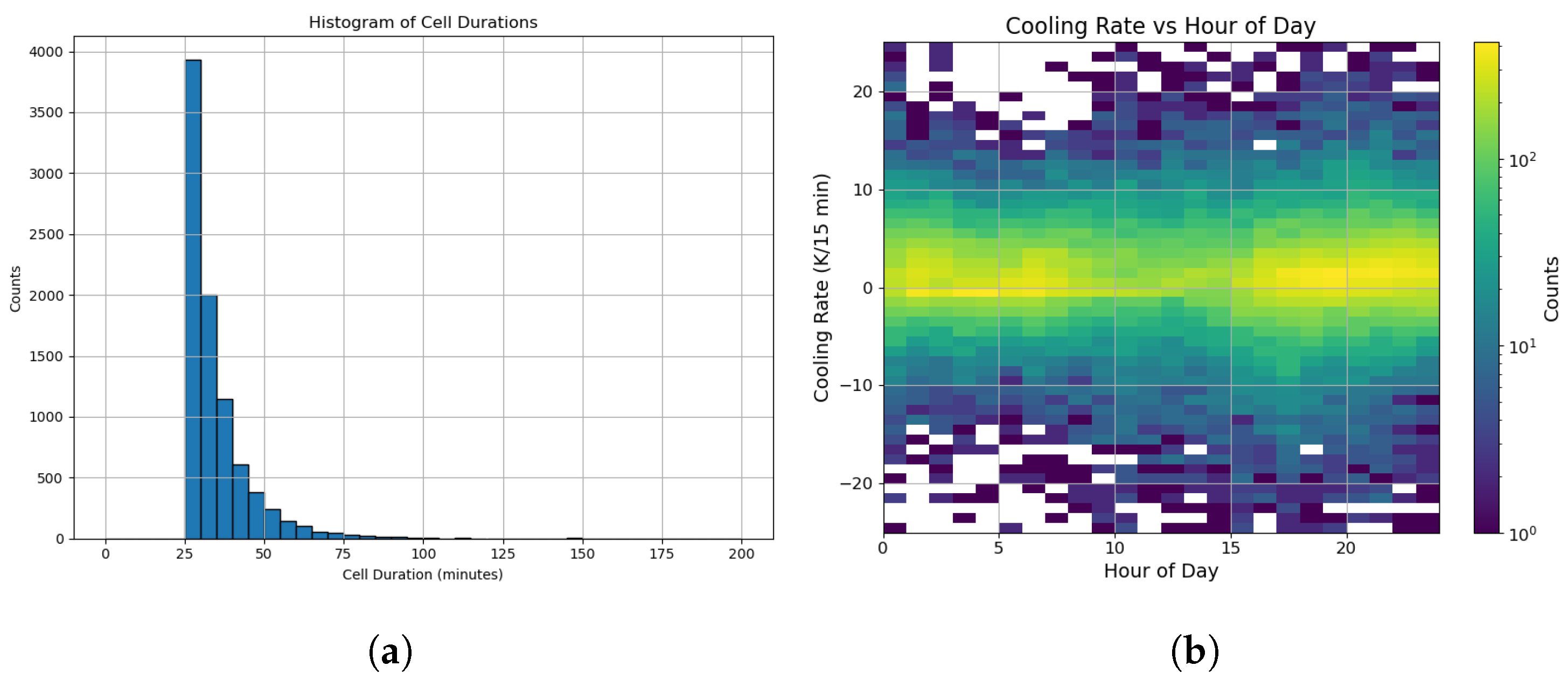
• Due to the coarse spatial resolution of IR geostationary sensors, NUBF can adversely affect the cloud detection and the magnitude of the cooling rate of the cell. As it is the horizontal resolution of the GOES IR channel 13 2 km, the cooling rates of convective cells with characteristic size comparable or finer than the GOES IR resolution can be seriously underestimated due to NUBF. In particular, convection initiation and final stages are difficult to detect using geostationary data only; the radar scans play a crucial role in detecting and tracking cells during these phases.
• The comparison between the satellite cloud-top cooling rate and the ground-based radar RHI scans for MAAS convective cell tracking data demonstrated that for extended and isolated cells, the cooling rate well represents radar echo top evolution, vertical velocity evolution, and elevated vertical velocity in the early stage of convective cells.
• The NWC SAF-GEO software demonstrates robustness and reliability in tracking mesoscale convective systems. However, its performance in detecting smaller-scale, early-stage convective activity is hindered by temporal resolution constraints and threshold limitations. Future improvements could include higher temporal frequency datasets and refined calibration techniques to enhance the detection of early convective development.
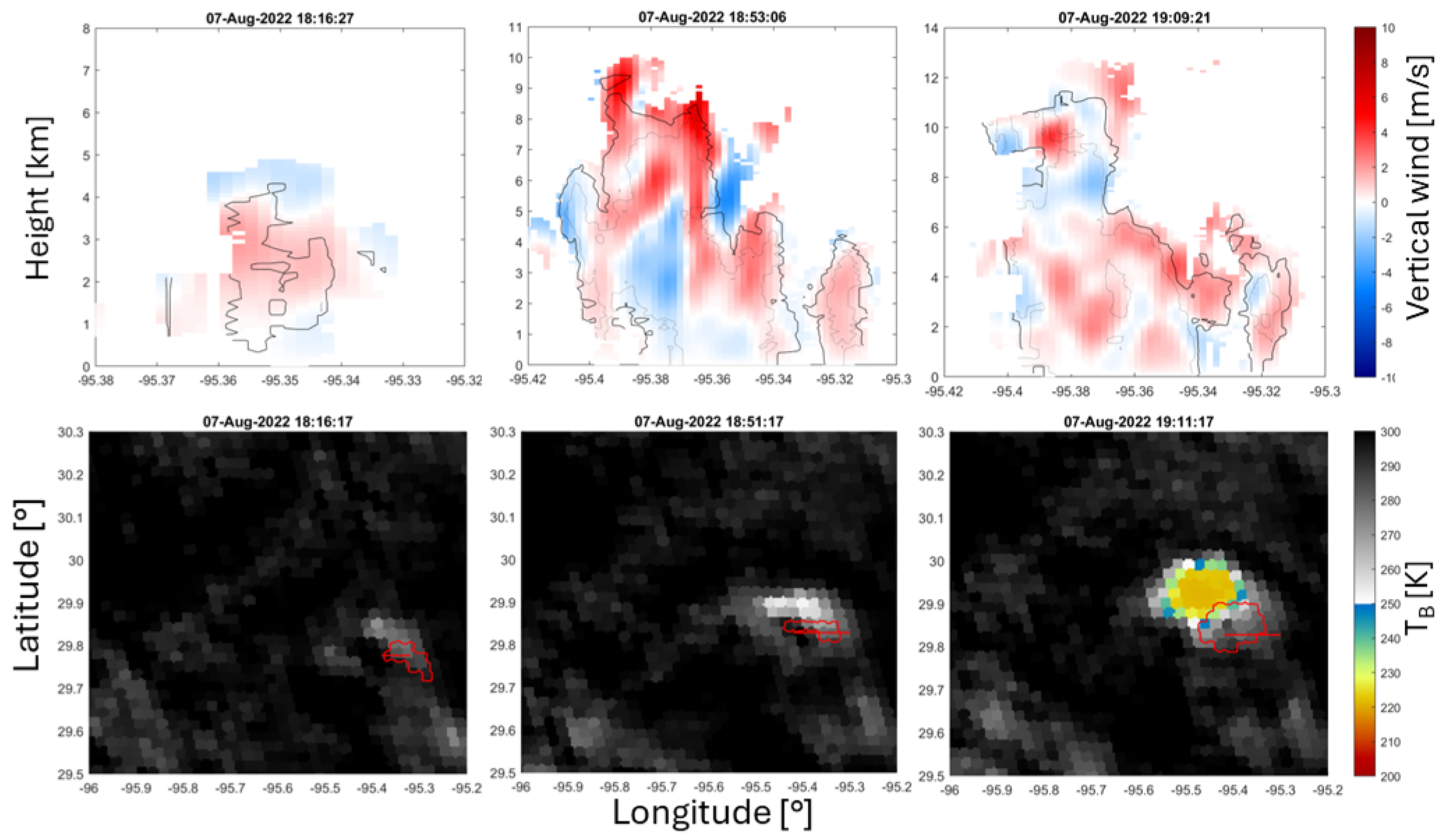
• The satellite cloud-top cooling rate was compared with the vertical velocity from multi-Doppler wind retrievals using the ground-based radar RHI scans for a selected case. The cooling rate generally captured the evolution of vertical velocity strength and the elevation of the velocity core until the cloud top attained $12 \mathrm{k}\mathrm{m}$ altitude. Variability with short time scale shown in the retrieved vertical velocity was not captured by the satellite: the satellite time and spatial resolutions are not sensitive to the short time scale cell evolution or small-scale spatial variability. However, it was also possible that the variability resulted from uncertainties in the multi-Doppler wind retrievals. Further analysis on more selected case studies will be needed for better comparisons with the wind retrievals.
• Although the uniqueness of the TRACER/ESCAPE field campaign dataset for studying convective updrafts, a number of sampling issues affecting the quality of the cells tracking with the radar arose. Given the complexity of the convective events and their spatiotemporal evolution, to have a good trade-off between the number of performed RHI scans and the time of acquisition and radar repositioning, often the results are coarse scans that do not follow the core of the cell properly. In addition, the choice of following a cell with the dedicated RHI scans can be affected by new cells forming in more advantageous locations for the radars or more promising ones: this results in a loss of continuity in time on the tracking, not allowing a good match with the geostationary observations.
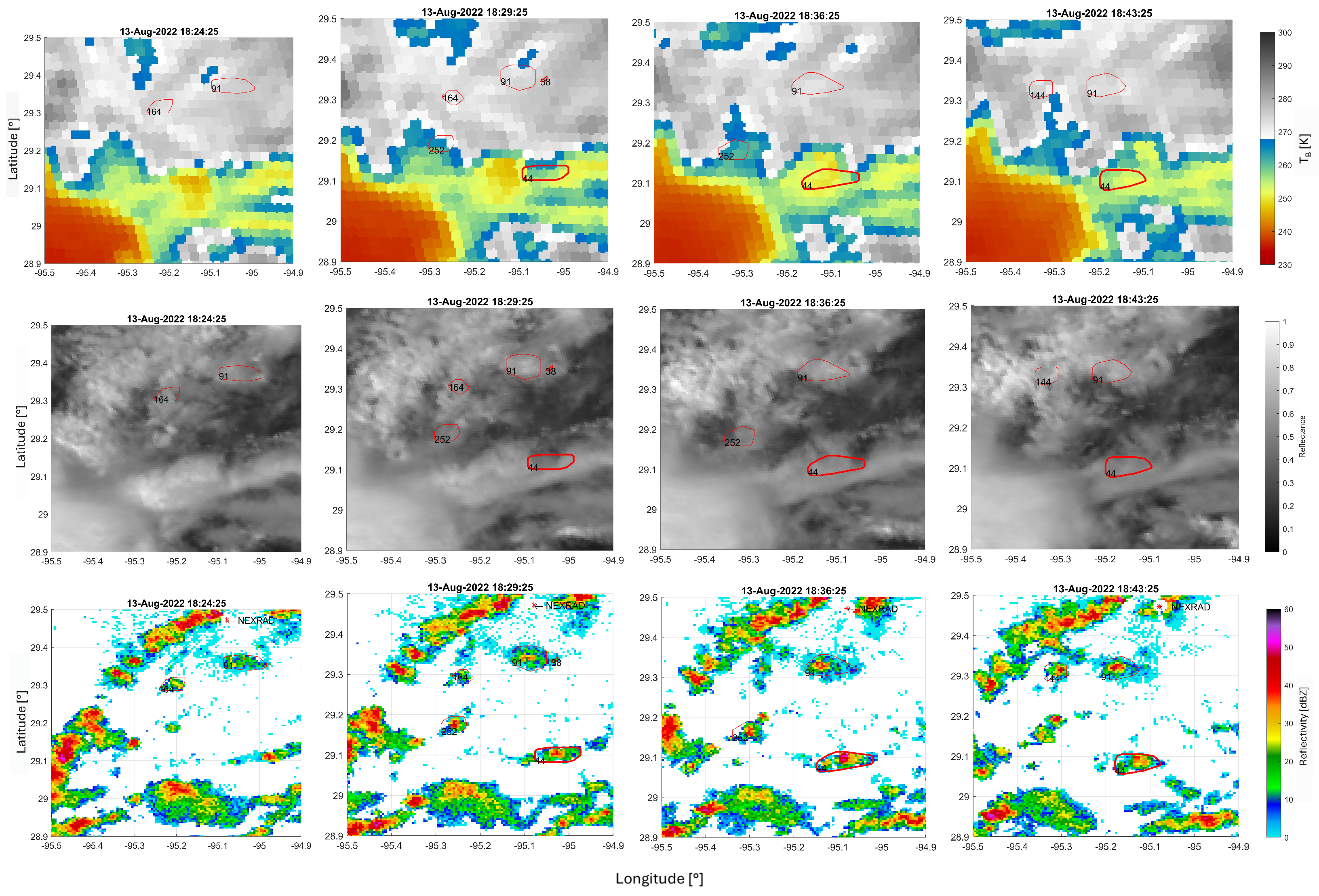
• Often, when observing organized convective systems, early developing cells with their cold anvil can mask later developing convection. Under such conditions, the geostationary sensor is blind to the cells developing beneath the anvil, and only ground-based radars are effective in detecting the convective cores.
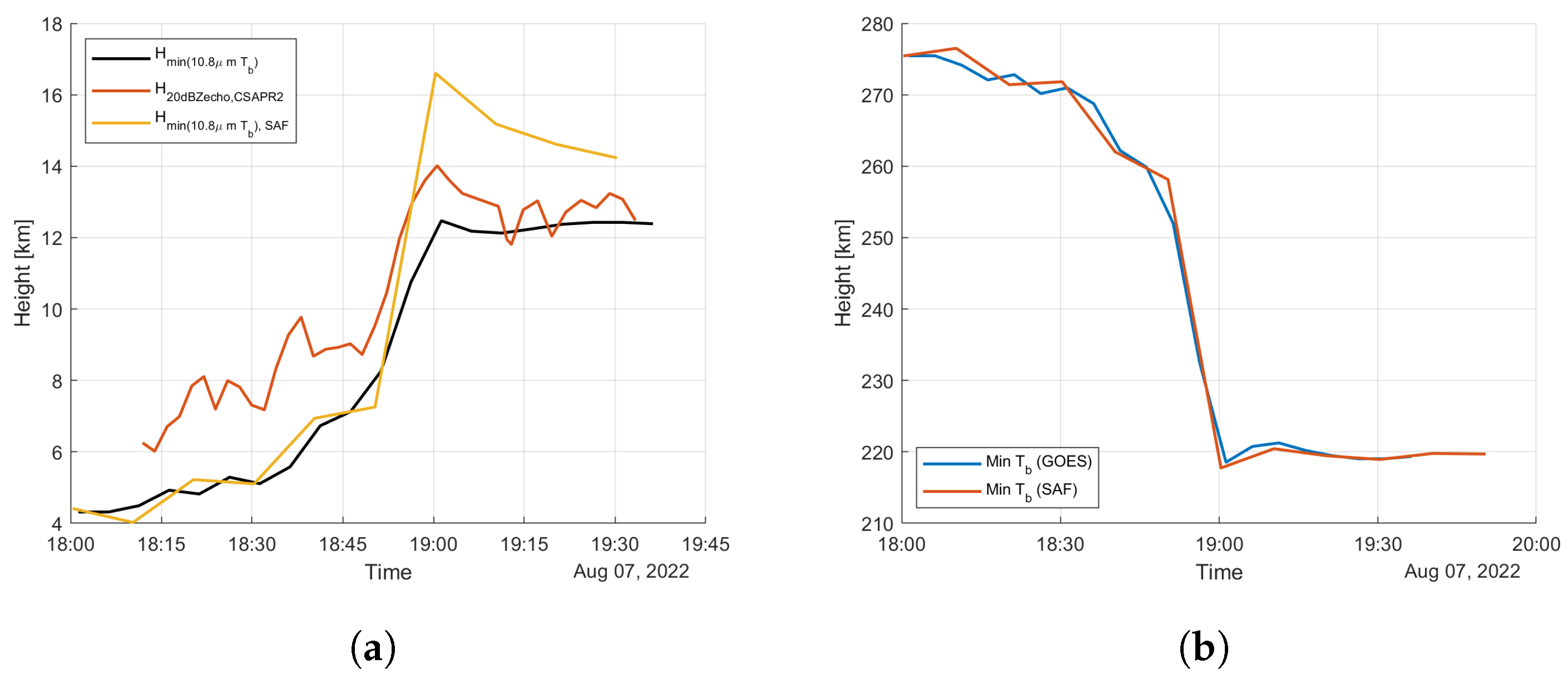
• Considering only longer tracked (at least 15 min) cells, there is a good agreement between the height of the 20 dBZ echo top of the NEXRAD radar and the CTH of the minimum $T_b^{IR}$ at low altitudes. However, when the CTH increases in height, the radar fails to observe the upper parts of the clouds.

Some opportunities for future work are discussed in the paper.

• During daytime, the issue encountered for the GEO-IR data due to NUBF can be flagged using the VIS channel of the GOES, which has a horizontal resolution of $0.5 \mathrm{k}\mathrm{m}$.
• The analysis should be extended to different locations and to different types of convective systems (e.g., MCS, hurricanes) to understand the capability of the proposed techniques for the study of convective cells developing in different environments.

Despite the aforementioned issues, the potential of the geostationary IR $T_b^{IR}$ to characterize convection, especially in the early phases, is clear. Thanks to their extended spatial and temporal coverage, geostationary data can enable statistical studies over bigger areas and longer periods than dedicated field campaigns.

The ground-based radar plays a very important role in detecting small cells and convection that is partially or completely not visible from geostationary sensors. The MAAS algorithm is being improved to better match the position of the cell’s core and for cell selection, also relying on geostationary IR cooling rates. A number of field campaigns planned for the coming years will enrich the current TRACER/ESCAPE dataset and test the improvements of the MAAS algorithm. Synergistic analysis of convection from geostationary passive and ground-based active instruments can unveil novel conclusions about the early-stage characterization of convective updraft.

References

1. Hartmann, D.L.; Hendon, H.H.; Houze, R.A. Some Implications of the Mesoscale Circulations in Tropical Cloud Clusters for Large-Scale Dynamics and Climate. J. Atmos. Sci. 1984, 41, 113–121. [Google Scholar] [CrossRef]
2. Sherwood, S.; Bony, S.; Dufresne, J.L. Spread in model climate sensitivity traced to atmospheric convective mixing. Nature 2014, 505, 37–42. [Google Scholar] [CrossRef] [PubMed]
3. Ladino, L.A.; Korolev, A.; Heckman, I.; Wolde, M.; Fridlind, A.M.; Ackerman, A.S. On the role of ice-nucleating aerosol in the formation of ice particles in tropical mesoscale convective systems. Geophys. Res. Lett. 2017, 44, 1574–1582. [Google Scholar] [CrossRef] [PubMed]
4. Lemone, M.A.; Zipser, E.J. Cumulonimbus vertical velocity events in GATE. Part I: Diameter, intensity and mass flux. J. Atmos. Sci. 1980, 37, 2444–2457. [Google Scholar] [CrossRef]
5. Kollias, P.; McFarquhar, G.M.; Bruning, E.; DeMott, P.J.; Kumjian, M.R.; Lawson, P.; Lebo, Z.; Logan, T.; Lombardo, K.; Oue, M.; et al. Experiment of Sea Breeze Convection, Aerosols, Precipitation and Environment (ESCAPE). Bull. Am. Meteorol. Soc. 2024, 106, E310–E332. [Google Scholar] [CrossRef]
6. Williams, C.R. Vertical Air Motion Retrieved from Dual-Frequency Profiler Observations. J. Atmos. Ocean. Technol. 2012, 29, 1471–1480. [Google Scholar] [CrossRef]
7. Giangrande, S.E.; Collis, S.M.; Straka, J.M.; Protat, A.; Williams, C.R.; Krueger, S.K. A Summary of Convective-Core Vertical Velocity Properties Using ARM UHF Wind Profilers in Oklahoma. J. Appl. Meteorol. Climatol. 2013, 52, 2278–2295. [Google Scholar] [CrossRef]
8. Kumar, V.V.; Jakob, C.; Protat, A.; Williams, C.R.; May, P.T. Mass-Flux Characteristics of Tropical Cumulus Clouds from Wind Profiler Observations at Darwin, Australia. J. Atmos. Sci. 2015, 72, 1837–1855. [Google Scholar] [CrossRef]
9. Junyent, F.; Chandrasekar, V.; McLaughlin, D.; Insanic, E.; Bharadwaj, N. The CASA Integrated Project 1 Networked Radar System. J. Atmos. Ocean. Technol. 2010, 27, 61–78. [Google Scholar] [CrossRef]
10. North, K.W.; Oue, M.; Kollias, P.; Giangrande, S.E.; Collis, S.M.; Potvin, C.K. Vertical air motion retrievals in deep convective clouds using the ARM scanning radar network in Oklahoma during MC3E. Atmos. Meas. Tech. 2017, 10, 2785–2806. [Google Scholar] [CrossRef]
11. Protat, A.; Zawadzki, I. A Variational Method for Real-Time Retrieval of Three-Dimensional Wind Field from Multiple-Doppler Bistatic Radar Network Data. J. Atmos. Ocean. Technol. 1999, 16, 432–449. [Google Scholar] [CrossRef]
12. Bell, M.M.; Montgomery, M.T.; Emanuel, K.A. Air-Sea Enthalpy and Momentum Exchange at Major Hurricane Wind Speeds Observed during CBLAST. J. Atmos. Sci. 2012, 69, 3197–3222. [Google Scholar] [CrossRef]
13. Potvin, C.K.; Wicker, L.J.; Shapiro, A. Assessing Errors in Variational Dual-Doppler Wind Syntheses of Supercell Thunderstorms Observed by Storm-Scale Mobile Radars. J. Atmos. Ocean. Technol. 2012, 29, 1009–1025. [Google Scholar] [CrossRef]
14. Oue, M.; Kollias, P.; Shapiro, A.; Tatarevic, A.; Matsui, T. Investigation of observational error sources in multi-Doppler-radar three-dimensional variational vertical air motion retrievals. Atmos. Meas. Tech. 2019, 12, 1999–2018. [Google Scholar] [CrossRef]
15. Illingworth, A.J.; Barker, H.W.; Beljaars, A.; Ceccaldi, M.; Chepfer, H.; Clerbaux, N.; Cole, J.; Delanoë, J.; Domenech, C.; Donovan, D.P.; et al. The EarthCARE Satellite: The Next Step Forward in Global Measurements of Clouds, Aerosols, Precipitation, and Radiation. Bull. Am. Meteorol. Soc. 2015, 96, 1311–1332. [Google Scholar] [CrossRef]
16. Kollias, P.; Puidgomènech Treserras, B.; Battaglia, A.; Borque, P.; Tatarevic, A. Processing reflectivity and Doppler velocity from EarthCARE’s cloud profiling radar: The C-FMR, C-CD and C-APC products. Atmos. Meas. Tech. 2022, 16, 1901–1914. [Google Scholar] [CrossRef]
17. Stephens, G.L.; van den Heever, S.C.; Haddad, Z.S.; Posselt, D.J.; Storer, R.L.; Grant, L.D.; Sy, O.O.; Rao, T.N.; Tanelli, S.; Peral, E. A Distributed Small Satellite Approach for Measuring Convective Transports in the Earth’s Atmosphere. IEEE Geosci. Remote Sens. Lett. 2020, 58, 4–13. [Google Scholar] [CrossRef]
18. Van der Heever, S. NASA Selects New Mission to Study Storms, Impacts on Climate Models. NASA Earth; 2021. Available online: https://www.nasa.gov/press-release/nasa-selects-new-mission-to-study-storms-impacts-on-climate-models (accessed on 20 March 2024).
19. Hartung, D.C.; Sieglaff, J.M.; Cronce, L.M.; Feltz, W.F. An Intercomparison of UW Cloud-Top Cooling Rates with WSR-88D Radar Data. Weather Forecast. 2013, 28, 463–480. [Google Scholar] [CrossRef]
20. Adler, R.F.; Fenn, D.D. Thunderstorm Intensity as Determined from Satellite Data. J. Appl. Meteorol. Climatol. 1979, 18, 502–517. [Google Scholar] [CrossRef]
21. Adler, R.F.; Fenn, D.D. Thunderstorm Vertical Velocities Estimated from Satellite Data. J. Atmos. Sci. 1979, 36, 1747–1754. [Google Scholar] [CrossRef]
22. Bikos, D.; Weaver, J.F.; Braun, J. The Role of GOES Satellite Imagery in Tracking Low-Level Moisture. Weather Forecast. 2006, 21, 232–241. [Google Scholar] [CrossRef]
23. Bedka, K.; Brunner, J.; Dworak, R.; Feltz, W.; Otkin, J.; Greenwald, T. Objective Satellite-Based Detection of Overshooting Tops Using Infrared Window Channel Brightness Temperature Gradients. J. Appl. Meteorol. Climatol. 2010, 49, 181–202. [Google Scholar] [CrossRef]
24. Hamada, A.; Takayabu, Y.N. Convective cloud top vertical velocity estimated from geostationary satellite rapid-scan measurements. Geophys. Res. Lett. 2016, 43, 5435–5441. [Google Scholar] [CrossRef]
25. Sieglaff, J.M.; Cronce, L.M.; Feltz, W.F.; Bedka, K.M.; Pavolonis, M.J.; Heidinger, A.K. Nowcasting Convective Storm Initiation Using Satellite-Based Box-Averaged Cloud-Top Cooling and Cloud-Type Trends. J. Appl. Meteorol. Climatol. 2011, 50, 110–126. [Google Scholar] [CrossRef]
26. Walker, J.R.; MacKenzie, W.M.; Mecikalski, J.R.; Jewett, C.P. An Enhanced Geostationary Satellite–Based Convective Initiation Algorithm for 0–2-h Nowcasting with Object Tracking. J. Appl. Meteorol. Climatol. 2012, 51, 1931–1949. [Google Scholar] [CrossRef]
27. Liu, Z.; Min, M.; Li, J.; Sun, F.; Di, D.; Ai, Y.; Li, Z.; Qin, D.; Li, G.; Lin, Y.; et al. Local Severe Storm Tracking and Warning in Pre-Convection Stage from the New Generation Geostationary Weather Satellite Measurements. Remote Sens. 2019, 11, 383. [Google Scholar] [CrossRef]
28. Lee, Y.; Kummerow, C.D.; Zupanski, M. A simplified method for the detection of convection using high-resolution imagery from GOES-16. Atmos. Meas. Tech. 2021, 14, 3755–3771. [Google Scholar] [CrossRef]
29. Lee, Y.; Kummerow, C.D.; Ebert-Uphoff, I. Applying machine learning methods to detect convection using Geostationary Operational Environmental Satellite-16 (GOES-16) advanced baseline imager (ABI) data. Atmos. Meas. Tech. 2021, 14, 2699–2716. [Google Scholar] [CrossRef]
30. Hong, Y.; Nesbitt, S.W.; Trapp, R.J.; Di Girolamo, L. Near-global distributions of overshooting tops derived from Terra and Aqua MODIS observations. Atmos. Meas. Tech. 2023, 16, 1391–1406. [Google Scholar] [CrossRef]
31. Cooney, J.W.; Bedka, K.M.; Bowman, K.P.; Khlopenkov, K.V.; Itterly, K. Comparing Tropopause-Penetrating Convection Identifications Derived From NEXRAD and GOES Over the Contiguous United States. J. Geophys. Res. Atmos. 2021, 126, e2020JD034319. [Google Scholar] [CrossRef]
32. Jensen, M.P.; Flynn, J.H.; Judd, L.M.; Kollias, P.; Kuang, C.; Mcfarquhar, G.; Nadkarni, R.; Powers, H.; Sullivan, J. A Succession of Cloud, Precipitation, Aerosol, and Air Quality Field Experiments in the Coastal Urban Environment. Bull. Am. Meteorol. Soc. 2022, 103, 103–105. [Google Scholar] [CrossRef]
33. Lamer, K.; Kollias, P.; Luke, E.P.; Treserras, B.P.; Oue, M.; Dolan, B. Multisensor Agile Adaptive Sampling (MAAS): A Methodology to Collect Radar Observations of Convective Cell Life Cycle. J. Atmos. Ocean. Technol. 2023, 40, 1509–1522. [Google Scholar] [CrossRef]
34. Hu, J.; Rosenfeld, D.; Zrnic, D.; Williams, E.; Zhang, P.; Snyder, J.C.; Ryzhkov, A.; Hashimshoni, E.; Zhang, R.; Weitz, R. Tracking and characterization of convective cells through their maturation into stratiform storm elements using polarimetric radar and lightning detection. Atmos. Res. 2019, 226, 192–207. [Google Scholar] [CrossRef]
35. Oue, M.; Saleeby, S.M.; Marinescu, P.J.; Kollias, P.; van den Heever, S.C. Optimizing radar scan strategies for tracking isolated deep convection using observing system simulation experiments. Atmos. Meas. Tech. 2022, 15, 4931–4950. [Google Scholar] [CrossRef]
36. Kollias, P.; Luke, E.; Oue, M.; Lamer, K. Agile Adaptive Radar Sampling of Fast-Evolving Atmospheric Phenomena Guided by Satellite Imagery and Surface Cameras. Geophys. Res. Lett. 2020, 47, e2020GL088440. [Google Scholar] [CrossRef]
37. Atmospheric Radiation Measurement (ARM) User Facility. Tracking Aerosol Convection Interactions Experiment (TRACER). 2021–2022. Available online: https://www.arm.gov/research/campaigns/amf2021tracer (accessed on 15 May 2025).
38. Roberts, R.D.; Rutledge, S. Nowcasting Storm Initiation and Growth Using GOES-8 and WSR-88D Data. Weather Forecast. 2003, 18, 562–584. [Google Scholar] [CrossRef]
39. Henderson, D.S.; Otkin, J.A.; Mecikalski, J.R. Evaluating Convective Initiation in High-Resolution Numerical Weather Prediction Models Using GOES-16 Infrared Brightness Temperatures. Mon. Weather Rev. 2021, 149, 1153–1172. [Google Scholar] [CrossRef]
40. Bieliński, T. A Parallax Shift Effect Correction Based on Cloud Height for Geostationary Satellites and Radar Observations. Remote Sens. 2020, 12, 365. [Google Scholar] [CrossRef]
41. Radová, M.; Seidl, J. PARALLAX APPLICATIONS WHEN COMPARING RADAR AND SATELLITE DATA. In Proceedings of the Meteorological Satellite Conference, Darmstadt, Germany, 8–12 September 2008. [Google Scholar]
42. Bernal Ayala, A.; Gerth, J.; Schmit, T.; Lindstrom, S.; Nelson, J. Parallax Shift in GOES ABI Data. J. Oper. Meteorol. 2023, 11, 14–23. [Google Scholar] [CrossRef]
43. Oue, M.; Treserras, B.P.; Luke, E.P.; Kollias, P. CSAPR2 Optimized Convective Cell Tracking Data During TRACER; Office of Scientific and Technical Information, U.S. Department of Energy: Washington, DC, USA, 2023.
44. Oue, M. ESCAPE: CHIVO Radar Data; Version 0.1 [PRELIMINARY]; UCAR/NCAR-Earth Observing Laboratory: Boulder, CO, USA, 2023. [Google Scholar]
45. Barnes, S.L. A Technique for Maximizing Details in Numerical Weather Map Analysis. J. Appl. Meteorol. Climatol. 1964, 3, 396–409. [Google Scholar] [CrossRef]
46. Heikenfeld, M.; Marinescu, P.J.; Christensen, M.; Watson-Parris, D.; Senf, F.; van den Heever, S.C.; Stier, P. tobac 1.2: Towards a flexible framework for tracking and analysis of clouds in diverse datasets. Geosci. Model Dev. 2019, 12, 4551–4570. [Google Scholar] [CrossRef]
47. Sokolowsky, G.A.; Freeman, S.W.; Jones, W.K.; Kukulies, J.; Senf, F.; Marinescu, P.J.; Heikenfeld, M.; Brunner, K.N.; Bruning, E.C.; Collis, S.M.; et al. Tobac V1.5: Introducing Fast 3D Tracking, Splits Mergers, Other Enhancements Identifying Analysing Meteorological Phenomena. Geosci. Model Dev. 2024, 17, 5309–5330. [Google Scholar] [CrossRef]
Figure 1. Location of ground-based radars during the TRACER/ESCAPE field campaign. Red circles are centered on CSAPR2 and CHIVO radar locations, respectively, with 75 k m radius.
Remotesensing 17 02621 g001
Figure 2. (a) Schematic of the temporal evolution of a convective system. The updraft fills only a fraction of the grid pixels. (b) Temporal evolution of the cloud cooling rate for different cloud fractions (CF) as indicated in the legend. A cooling rate of 30 K/15 min is assumed for the convective cell. The presence of NUBF causes a significant underestimation of updraft strength.
Remotesensing 17 02621 g002
Figure 3. Subsequent images depicting the time evolution of a convective cell that developed on 7 August 2022. The colors represent the maximum reflectivity in the column of the NEXRAD volume scans; the red contour is the parallax-corrected IR area that has a brightness temperature lower than the IR T b I R minimum within the cell increased by 10   K . Black contours represent the IR brightness temperature from the GOES satellite, not corrected for the parallax (dashed line minimum T b I R + 10   K , solid line minimum T b I R + 30   K ). The green lines are the RHI lines from the CSAPR2 dedicated scans. The blue lines are the RHI lines recorded by the CHIVO radar.
Remotesensing 17 02621 g003
Figure 4. Time-series of geostationary and radar ground-based characteristics of the case study selected on 7 August 2022 from 6 pm UTC. (a) shows the minimum of the brightness temperature (cyan line) recorded within the cell by the IR channel of the geostationary radiometer; the orange line is the T b I R < 230   K area (right vertical axis). (b) compares the height of the minimum T b I R within the cell on the IR image (black line) and the maximum height of the 20, 30, and 40 dBZ levels from the CSAPR2 radar RHI scans. The red boxes identify features that are commented on in the text.
Remotesensing 17 02621 g004
Figure 5. RHI scan bundles (with six different azimuthal angles per bundle) recorded by CSAPR2 radar around the times 18h17, 18h38, and 19h00 UTC on 7 August 2022.
Remotesensing 17 02621 g005
Figure 6. Time series of geostationary T b I R of the case study selected on 7 August 2022 after 6 pm UTC, corrected for the parallax. The red contours represent the cloud base (solid line) and the cloud top (dashed line) detected by the NWC SAF GEO software. The software detected the cell for the first time at 19h20, assigning a growing stage. The software keeps following this cell until 21h00.
Remotesensing 17 02621 g006
Figure 7. Time-series of geostationary and radar ground-based characteristics of the case study selected on 7 August 2022 from 6 pm UTC. (a) compares the height of the minimum T b I R within the cell on the IR image (black line) and the maximum height of the 20 dBZ level from the CSAPR2 radar RHI scans (orange line) to the cloud-top product, parallax corrected, from SAF software (yellow line). (b) shows the minimum of the brightness temperature (cyan line) recorded within the cell by the IR channel of the geostationary radiometer and from the parallax-corrected product from SAF software (orange line).
Remotesensing 17 02621 g007
Figure 8. Upper panels: profiles of the 3D vertical wind field at fixed latitude (left to right: 29.83°, 29.88°, 29.91°) of echoes exceeding 20 dBZ. The black solid and dotted lines correspond to the 30 dBZ and 40 dBZ reflectivity contours, respectively. Lower panels: quasi-coincident GOES 10.8   μ m   T b I R for the area surrounding the convective cell tracked by the radars with acquisition time detailed in the title. Red lines correspond to the contours where T b I R = m i n c e l l ( T b I R ) + 10   K , corrected for the parallax. The red horizontal lines are the ground projections of the profiles shown in the upper panels.
Remotesensing 17 02621 g008
Figure 9. (a) Temporal evolution of different parameters (as indicated in the legend) describing the evolution of the convective cell shown in Figure 3, Figure 4 and Figure 5 and Figure 8. The black line is derived from the GEO-IR T b I R by the closest temperature profile sounding, whereas the other lines are based on radar observables of the 3D structure of the convective cell. (b) The time derivative of the height of T b I R minimum (cyan line) is compared to the maximum vertical velocity retrieved by the dual Doppler radar measurements within the cell (orange line).
Remotesensing 17 02621 g009
Figure 10. (Top row) a sequence of T b I R from GOES channel 13, with a time resolution of 5 min. Red contours represent the cells identified as trackable by the NEXRAD in the area, shifted on the GEO-image after the parallax correction. The thicker contours refer to cells 55 and 73, discussed as case studies. (Bottom row) time evolution of the maximum column reflectivity derived from the NEXRAD volume scans, roughly matching the time stamps of the GEO-IR images. The red contours are the same as in the row above.
Remotesensing 17 02621 g010
Figure 11. (Top row) 20 min time evolution of the IR brightness temperature from GOES channel 13. Red contours represent the trackable cells in the area, positioned after the parallax correction. The thicker red contour refers to cell 44, discussed in detail. Mid row: 20 min time evolution of the reflectances from GOES channel 2. The red contours are as above. (Bottom row) time evolution of the maximum columnar reflectivity per pixel from the NEXRAD volume scans. The red contours are the same as the row above.
Remotesensing 17 02621 g011
Figure 12. (a) Histogram of the tracking duration of all cells included in the trackable set. (b) Density plot comparing the cloud-top height of the pixel with maximum VIL (seen by NEXRAD) and cloud-top height of the minimum brightness temperature pixel (on the GEO-IR).
Remotesensing 17 02621 g012
Figure 13. (a) Histogram of the tracking duration of all cells included in the trackable set. (b) Density plot comparing the cloud-top cooling rate of the minimum brightness temperature pixel (on the GEO-IR) along the hours of the day.
Remotesensing 17 02621 g013
Disclaimer/Publisher’s Note: The statements, opinions and data contained in all publications are solely those of the individual author(s) and contributor(s) and not of MDPI and/or the editor(s). MDPI and/or the editor(s) disclaim responsibility for any injury to people or property resulting from any ideas, methods, instructions or products referred to in the content.