CCDR: Combining Channel-Wise Convolutional Local Perception, Detachable Self-Attention, and a Residual Feedforward Network for PolSAR Image Classification

Abstract

In the task of PolSAR image classification, effectively utilizing convolutional neural networks and vision transformer models with limited labeled data poses a critical challenge. This article proposes a novel method for PolSAR image classification that combines channel-wise convolutional local perception, detachable self-attention, and a residual feedforward network. Specifically, the proposed method comprises several key modules. In the channel-wise convolutional local perception module, channel-wise convolution operations enable accurate extraction of local features from different channels of PolSAR images. The local residual connections further enhance these extracted features, providing more discriminative information for subsequent processing. Additionally, the detachable self-attention mechanism plays a pivotal role: it facilitates effective interaction between local and global information, enabling the model to comprehensively perceive features across different scales, thereby improving classification accuracy and robustness. Subsequently, replacing the conventional feedforward network with a residual feedforward network that incorporates residual structures aids the model in better representing local features, further enhances the capability of cross-layer gradient propagation, and effectively alleviates the problem of vanishing gradients during the training of deep networks. In the final classification stage, two fully connected layers with dropout prevent overfitting, while softmax generates predictions. The proposed method was validated on the AIRSAR Flevoland, RADARSAT-2 San Francisco, and RADARSAT-2 Xi’an datasets. The experimental results demonstrate that the proposed method can attain a high level of classification performance even with a limited amount of labeled data, and the model is relatively stable. Furthermore, the proposed method has lower computational costs than comparative methods.

1. Introduction

Synthetic Aperture Radar (SAR) is an active microwave remote sensing system. It observes targets by transmitting high-power electromagnetic pulses to them and then receiving the sequentially reflected backscattered signals [1]. The electromagnetic wave of the microwave band has strong penetrating power and can detect hidden targets covered by vegetation. SAR [2] has all-weather, day-and-night imaging capability, which allows it to stably obtain high-resolution images in complex environments such as cloudy conditions, rainy conditions, or dark nights. It is suitable for long-term monitoring tasks of Earth observations [3]. Polarimetric Synthetic Aperture Radar (PolSAR) is a multi-polarization system distinct from optical systems. By utilizing four different modes, it captures a wide range of scattering information, allowing for detailed extraction of target features, including scattering echo amplitude, phase, frequency characteristics, and polarization properties [4,5]. In applications, the advantage of PolSAR lies in its ability to overcome susceptibility to lighting and weather changes, enabling its use across diverse tasks, including ground feature classification, land-cover monitoring, forest structure analysis, and marine ice and snow monitoring [6,7,8]. The PolSAR image classification task involves classifying pixels into multiple categories based on certain rules, which can be applied in both military and civilian fields. In military applications, PolSAR image classification can be used to select favorable terrain, locate key targets, and provide intelligence support for precise strikes. In civilian applications, PolSAR image classification updates regional land-cover information on a large scale, serving vegetation surveys, urban planning, disaster monitoring, etc. [9]. Common objects in PolSAR images include land, buildings, water bodies, sandy areas, urban areas, vegetation, roads, and bridges [10,11]. PolSAR image classification has emerged as one of the research hotspots in the field of SAR remote sensing.

In recent years, deep learning methods have been widely used as efficient computational tools for PolSAR image classification tasks [12,13]; for example, models such as multi-layer metric networks, adversarial reconstruction networks [14], stacked autoencoders [15,16], and convolutional neural networks [17]. Unlike traditional machine learning, deep learning relies on representation learning [18], which automatically extracts features by constructing multi-layer neural networks. Deep learning models transform the feature representations of samples in the original space into a new feature space through layer-by-layer feature transformation, making classification or prediction easier [9].

Nowadays, for representation learning in the field of remote sensing images, many researchers choose a convolutional neural network (CNN) as a carrier [19]. Das et al. [20] first explored the application of CNNs in PolSAR image classification, in which the six-dimensional real vector obtained from the polarization coherence matrix T is used as the original input. The network architecture consists of two convolutional layers, two dense layers, and a softmax classifier for classification. Since the first application of CNNs in the field of PolSAR images, numerous CNN variants for this domain have been proposed. As a unique feature of PolSAR images, phase information plays a vital role in applications such as target classification and recognition, while traditional CNNs struggle to effectively extract phase information. To address this issue, researchers have explored the application of complex-valued convolutional neural networks (CV-CNNs) in the field of PolSAR image classification. Zhang et al. [21] extended all components of the CNN to the complex domain, significantly reducing classification errors. Chen and Tao [22] proposed a polarization-feature-driven deep CNN classification scheme. The core idea of this scheme combines expert knowledge of target scattering mechanism interpretation and polar coordinate feature mining to assist in the training of a deep CNN classifier under the condition of limited training samples, enhancing classification performance. However, as the application of convolutional neural networks (CNNs) in PolSAR image classification continues to advance, the scarcity of labeled data poses a significant obstacle to further enhancing the performance of deep learning algorithms [23]. Additionally, although CNNs can learn abstract features in PolSAR images well, each convolution kernel is limited to a fixed, small region. It is difficult for a single CNN to effectively extract globally relevant information in PolSAR images. This presents a barrier to further improvement of CNN-based PolSAR image classification methods.

The transformer model proposed by [24] was initially widely applied to natural language processing tasks and has since achieved significant breakthroughs in the field of computer vision. Specifically, the transformer architecture consists of two main components: the encoder, which processes the input data, and the decoder, which generates the output data. Furthermore, the self-attention mechanism lies at the core of the transformer, enabling it to capture global dependencies among individual elements in a sequence. By calculating attention weights across all positions in the sequence, the model has the flexibility to focus on the most relevant information [25]. In recent years, attention-based techniques have been widely applied in PolSAR image classification to enhance performance. These methods prioritize the most important features over uniform processing of the entire input, allowing models to emphasize critical information more effectively while minimizing the influence of less relevant features. Hua et al. [26] designed a PolSAR image classification algorithm based on a spatial weighted attention mechanism to select more informative spatial information.

Dosovitskiy et al. [27] proposed the application of the vision transformer (ViT) model in the field of computer vision, in which image patches replace words in a transformer for self-attention calculation, enabling the model to directly capture global relationships. Dong et al. [28] first explored the application of the ViT model in PolSAR image classification, using self-attention instead of a convolution operation and converting the scope of attention from local information to long-distance interactive information to address the inductive bias inherent in CNNs. They then verified the effectiveness of the self-attention mechanism through experiments. In addition, the application of modular design in deep learning also provides an efficient solution for PolSAR image classification tasks. For instance, Wang et al. [29] proposed a ViT-based MCPT classification model, which used mixed-depth convolutional tokenization to replace the learned linear projection in the original ViT to obtain patch embeddings, and introduced parallel encoders to effectively reduce the depth of the network without affecting the classification effect. In order to fully promote the application of the CNN–ViT fusion method for PolSAR image classification, Wang et al. [30] proposed a multi-granularity hybrid CNN–ViT model based on external tokens and a cross-attention method. This method realizes the interaction of multiscale features of PolSAR data through the multi-granularity attention and cross-attention feature fusion modules. Although ViT has been widely studied and applied in the field of remote sensing, there are still fewer ViT-based PolSAR image classification methods than CNN-based methods. The ViT method lacks the ability to extract local features and requires a large amount of computational resources to calculate global attention. Although the CNN–ViT method can better utilize the local feature extraction ability of CNNs and the global information acquisition ability of ViTs, it faces challenges in balancing the relationship between CNNs and ViTs and incurs high computational costs.

In current applications of deep learning in PolSAR image classification, existing deep learning models face two core challenges: the scarcity of labeled data and the limitations of feature interaction. On the one hand, labeling PolSAR data is costly, and labeled samples are scarce. CNNs rely on a large amount of labeled data for feature generalization, making it difficult for them to effectively capture feature information with a limited amount of labeled data. On the other hand, although ViTs can establish global dependencies through the self-attention mechanism, their computation of global attention requires substantial computational resources to achieve high performance, and they simultaneously lack sufficient capability to extract local detailed features. To address these issues, this article proposes a method for PolSAR image classification that combines channel-wise convolutional local perception, detachable self-attention, and a residual feedforward network, along with a modularization strategy. In scenarios with limited labeled data, this model not only fully extracts feature information from different channels but also facilitates the interaction between local and global information. Meanwhile, the model incurs relatively low computational costs, providing strong support for applications in resource-constrained scenarios. The main contributions of this article are as follows:

• A channel-wise convolutional local perception (CCLP) module. The CCLP module consists of two parts: channel-wise convolution and local residual connections. Channel-wise convolution replaces the block embedding part in the original ViT by grouping channels and assigning convolution kernels of different sizes to each group to extract the feature information contained in different channels. Afterward, local residual connections are introduced to further capture local information from intermediate features, thereby improving the expressive power of the network.
• A detachable self-attention (DTA) mechanism. DTA is a window-based attention mechanism that includes chunk-wise self-attention and point-wise self-attention, which can sequentially implement local–global information interaction between chunks and reduce computational complexity by adopting a partitioning strategy.
• A residual feedforward network (ResFFN). Compared with traditional feedforward networks, ResFFN more effectively characterizes local features and further enhances the ability of gradients in cross-layer propagation by introducing residual structures.

The remainder of this article is organized as follows. Section 2 provides a brief technical background and a detailed description of the proposed approach. In Section 3, the experimental results are comprehensively introduced and analyzed. Section 4 discusses the different factors that affect model performance. Finally, Section 5 summarizes this thesis.

2. Proposed Method

This study adopts a simplified modular strategy and proposes a method for PolSAR image classification that combines channel-wise convolutional local perception, detachable self-attention, and a residual feedforward network (CCDR). The structure of CCDR is illustrated in Figure 1, which breaks down the PolSAR image processing task into pixel-centered input extraction, feature extraction, and classification prediction. As shown in Figure 1, the model consists of three main components. The first component is a channel-wise convolutional local perception module, which is used to extract local features from different channels in PolSAR images. The second component is the detachable self-attention mechanism, which facilitates the interaction between local and global image information. The third component is the residual feedforward network, designed to enhance gradient propagation capability by altering the placement of the residual connections. After feature extraction is completed, the captured features are classified, and the final classification result is obtained. By employing a simplified modular strategy, the proposed method not only improves classification performance but also reduces computational time.

Generally, the polarization information of PolSAR pixels is represented by the polarization coherence matrix T [31], which is given in Equation (1):

$$\begin{array}{c}\hfill \mathbf{T}=\left[\begin{array}{ccc}{T}_{11}& T_{12}& T_{13}\\ T_{21}& T_{22}& T_{23}\\ T_{31}& T_{32}& T_{33}\end{array}\right],\end{array}$$

(1)

where T is a complex conjugate matrix whose principal diagonals are real-valued elements. This coherence matrix T can be transformed into a nine-dimensional vector v, whose expression is given in Equation (2) [32]:

$$\begin{array}{c}\hfill v=\left[T_{11},T_{22},T_{33},Re\left(T_{12}\right),Re\left(T_{13}\right),Re\left(T_{23}\right),Im\left(T_{12}\right),Im\left(T_{13}\right),Im\left(T_{23}\right)\right],\end{array}$$

(2)

where Re(·) and Im(·)denote the real and imaginary parts, respectively. In this article, the nine-dimensional vector of PolSAR data is used as input. The initial form of the data can be expressed as ${\mathbb{R}}^{9 \times H \times W}$, where H and W represent the height and width of a PolSAR image, respectively. Pixels with a size of $p\times p$ are extracted as input data for feature extraction, which can be expressed as ${\mathbb{R}}^{(H \times W) \times 9 \times p \times p}$.

2.1. Channel-Wise Convolutional Local Perception

Recently, CNNs have been extensively applied and innovated in the field of image processing, yet the significance of their kernel size is often neglected. The emergence of depth-wise convolution not only addresses this problem but also reflects the broader trend of CNNs toward improving accuracy and efficiency. Depth-wise convolution subsequently spawned many popular variants, such as MobileNets [33], ShuffleNets, and EfficientNet [34]. Unlike ordinary CNNs, depth-wise convolution operates on each individual channel separately, effectively reducing computational costs. Tan and Le [35] systematically investigated the effects of different kernel sizes and proposed a mixed-depth convolution that combines multiple kernel sizes in a single convolution. In this article, a channel-wise convolutional local perception (CCLP) module is proposed based on mixed-depth convolution, which efficiently extracts local feature information from PolSAR images and lays the foundation for subsequent global feature extraction.

The channel-wise convolutional local perception module replaces the patch embedding module in the original ViT. ViT divides the image into fixed-sized patches, which overlook the internal structural information of the image and impose stringent requirements on the input resolution. However, the channel-wise convolutional local perception module ensures that the input resolution remains unaffected by the preset patch size, enabling it to meticulously capture features within PolSAR images. This module comprises two components: channel-wise convolution and local residual connections. Specifically, channel-wise convolution is employed to capture various features within PolSAR images by grouping channels and assigning convolution kernels of varying sizes to each group. Suppose that the input tensor X is divided into g groups of tensors $\left[x^{(c_1,h,w)},\dots ,x^{(c_g,h,w)}\right]$, where all virtual tensors x have the same spatial height h and width w, and the total channel size is equal to the channel of the original input tensor, that is, $c_1+c_2+\dots +c_g=c$. The number of channel groups g determines how many different types of convolution kernels are applied to the input tensor. Channel-wise convolution is equivalent to ordinary convolution when the number of blocks $g=1$. Since this article uses PolSAR data with nine channels, the number of groups is set to $g=3$, which means that all three channels are grouped together. In a single convolution, kernel sizes of 3 × 3, 5 × 5, and 7 × 7 are used for the grouped channels; the design of this multiscale convolution kernel allows it to extract features from different receptive fields, thereby capturing information within PolSAR images more comprehensively. After channel-wise convolution, the channel features obtained are connected by a local residual. Since the original ViT added a unique location code for each patch, the local relationship [36] and structural information [37] inside the patch were ignored. To alleviate these limitations, local residual connections are introduced to capture local information within intermediate features, which operate through a 3 × 3 convolution kernel. This type of local processing enables the model to recognize low-level information within the image, such as edges, corners, and textures. This low-level information is crucial for the classification of PolSAR images. For example, edge information can help distinguish the boundaries of different features. Meanwhile, texture information can reflect the surface characteristics of these features.

As shown in Figure 2, first, a PolSAR image block with a size of H × W × C is extracted as input data with the pixel as the center. The channels are then divided into three groups according to the number of channels in the PolSAR data. For each group, convolution kernels with sizes of 3 × 3, 5 × 5, and 7 × 7 are used, respectively, to generate feature maps. The local information is then extracted through the local residual connection consisting of a 3 × 3 convolution. The operation mechanism of the channel-wise convolutional local perception module can be defined as follows:

$$\begin{array}{c}\hfill X^{*}=CC\left(X\right),\end{array}$$

(3)

$$\begin{array}{c}\hfill CCLP\left(X\right)=X^{*}+LRC\left(X^{*}\right),\end{array}$$

(4)

where X represents the input of PolSAR image blocks with a size of H × W × C extracted from pixels, CCLP represents channel-wise convolutional local perception, CC represents channel-wise convolution, $X^{*}$ represents the output after channel-wise convolution, and $X^{*}$ serves as the input for the local residual connection. LRC stands for local residual connection.

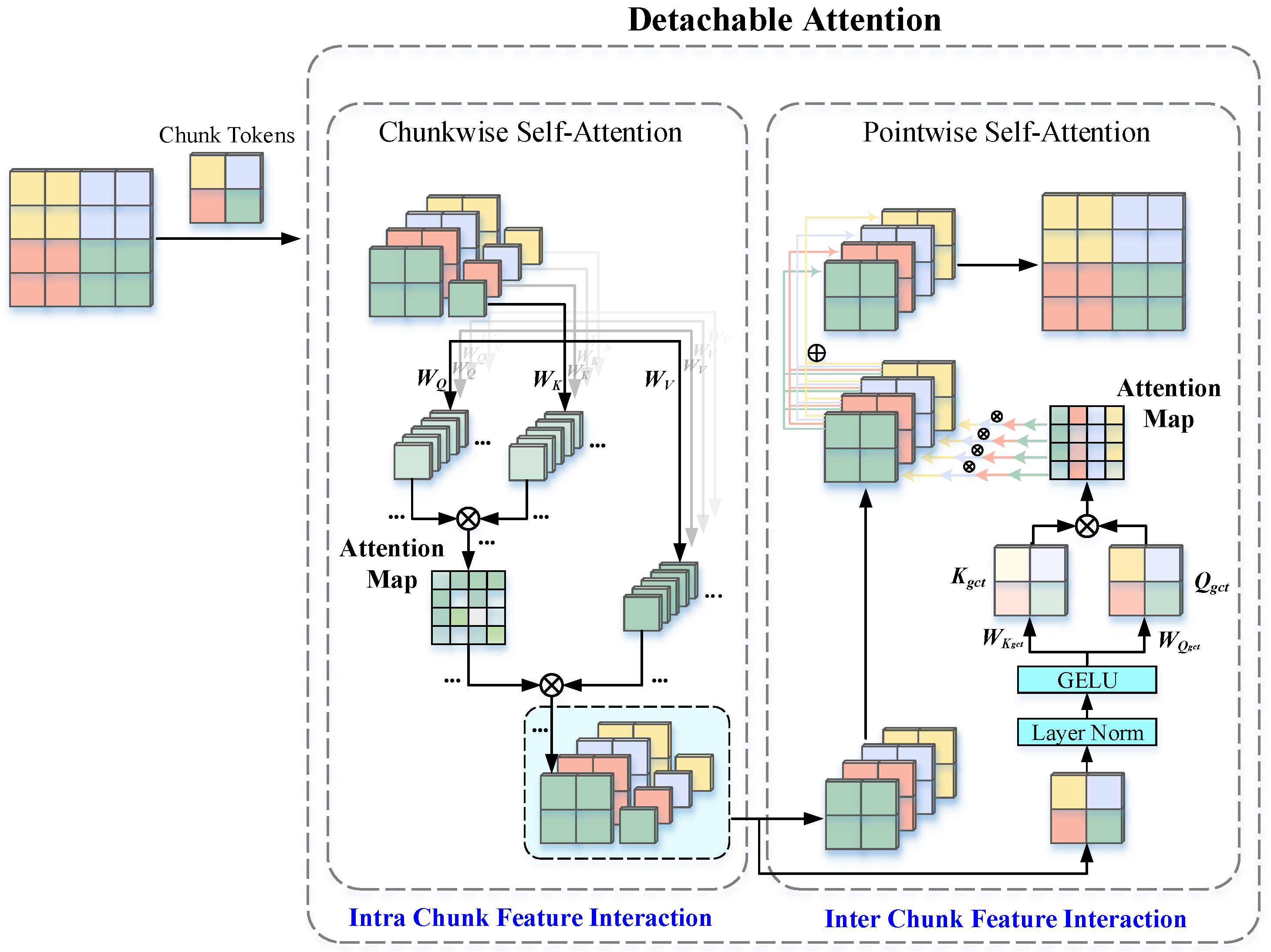
2.2. Detachable Self-Attention

The multi-head self-attention mechanism (MHSA) in the original ViT exhibits high computational complexity and lacks sensitivity to local information perception. In order to address these issues, the proposed method utilizes DTA to replace MHSA in the original ViT. Detachable self-attention (DTA) is a window-based self-attention mechanism that divides the input feature map into small windows (or regions), each containing a certain number of pixels and features. Self-attention is calculated within each window, thereby reducing computational complexity and increasing efficiency. DTA not only greatly reduces the burden of self-attention operations on tokens but also emphasizes the efficient extraction of global and local spatial features.

In the original ViT model, multi-head self-attention (MHSA) employs multiple sets of attention weights, with each set capable of learning different types of information [24]. Let the input feature matrix be denoted as $A_0\in {\mathbb{R}}^{H \times W \times C}$, where H, W, and C represent the height, width, and number of channels, respectively. The input features are transformed into a two-dimensional matrix $A_0\in {\mathbb{R}}^{HW \times C}$. Through three weight matrices—the query weight $W_Q$, key weight $W_K$, and value weight $W_V$—the input features are projected into query vectors Q, key vectors K, and value vectors V, where $W_Q,W_K,W_V\in {\mathbb{R}}^{(C \times C)}$. Sensitivity analysis represents a technical approach to evaluating how the output of a model responds to alterations in its input variables [38]. In practical research endeavors, conducting sensitivity analysis on weights such as the query weight $W_Q$, key weight $W_K$, and value weight $W_V$ enables a more accurate determination of features that are critical to the model, thereby offering valuable guidance for feature selection. The specific transformation formulas are given in Equation (5):

$$\begin{array}{c}\hfill Q=A\times W_Q,K=A\times W_K,V=A\times W_V,\end{array}$$

(5)

where $W_Q$, $W_K$, and $W_V$ are trainable parameters of the model. They are randomly initialized during model initialization and continuously optimized through backpropagation during the training process. These parameters serve as part of the linear transformation layers and are stored and updated as trainable tensors within the model. Although the attention mechanism formally processes all input features in a uniform manner, the attention weights calculated after mapping through $W_Q$, $W_K$, and $W_V$ are dynamic and data-dependent. These weights are computed based on the scaled dot-product attention mechanism, as shown in Equation (6):

$$\begin{array}{c}\hfill SA=\mathrm{Attention}(Q,K,V)=\mathrm{SoftMax}\left({\displaystyle \frac{Q{K}^T}{\sqrt{d_k}}}\right)V,\end{array}$$

(6)

where Q represents the features the model focuses on learning, K serves as a matching index to measure the correlation between different features, and V denotes the actual feature information that is learned and combined. $d_k$ represents the dimension of matrix K. By calculating the dot-product similarity between Q and K and performing normalization, the model can obtain the importance weights of each feature relative to the current query. Subsequently, it performs a weighted summation of the corresponding V, enabling the modeling of global context. This structure allows the model to automatically allocate varying degrees of attention to features based on the semantic relationships among inputs, thereby endowing the model with the capability of dynamic feature modeling and sensitivity expression. Through the learned attention distributions, implicit feature sensitivity modeling is achieved to a certain extent. MHSA utilizes multiple sets of self-attention weights and concatenates the results from each set, as shown in Equation (7):

$$\begin{array}{c}\hfill \mathrm{MHSA}(Q,K,V)=\mathrm{Concat}(S{A}_1,\dots ,S{A}_i,\dots ,S{A}_n)W,\end{array}$$

(7)

where $S{A}_i\in {\mathbb{R}}^{(HW \times C)/n}$, $W_i\in {\mathbb{R}}^{C \times C}$ represents the weight parameters and n represents the number of heads.

DTA consists of chunk-wise self-attention (CSA) and point-wise self-attention (PSA), which are connected in series to enable interaction between local information within individual chunks and global information across chunks. Unlike the original ViT, which computes self-attention uniformly across all token sequences in an image patch, DTA adopts a chunking strategy to reduce computational complexity while enhancing feature representation through a two-level self-attention mechanism. The structure of DTA is shown in Figure 3.

CSA divides the feature map into multiple feature submaps, generating a unique chunk token for each submap. Computing self-attention between each chunk token and its corresponding submap efficiently reduces the computational complexity of self-attention while effectively capturing local information. Specifically, the input feature map $Z\in {\mathbb{R}}^{H \times W \times C}$ is divided into N feature submaps $Z_j\in {\mathbb{R}}^{M \times M \times C}$ of spatial size $M\times M$, where $N={\displaystyle \frac{HW}{M^2}}$. Each feature submap is called a chunk, and each chunk generates a chunk token that encapsulates the core features of the chunk. The chunk tokens can be initialized to zero or a learnable random value. The purpose of introducing a chunk token is to provide a global representation within each chunk, thereby enabling local feature extraction from the entire feature map and assigning global weights to each chunk for the subsequent PSA process. Therefore, DTA implements both local and global feature extraction and interaction. Each chunk token attends to all the pixels within the corresponding chunk. Each chunk is flattened into a 2D sequence $Z_j\in {\mathbb{R}}^{M^2 \times C}$ along the spatial dimension. Subsequently, $Z_j$ is concatenated with the chunk token along the sequence dimension, resulting in $z_j^{\prime }\in {\mathbb{R}}^{M^{\prime } \times C}$. Through linear projection using different learnable weight matrices $W_Q^{\prime },W_K^{\prime },W_V^{\prime }\in {\mathbb{R}}^{(C \times C)}$, $Q_j$, $K_j$, and $V_j$ are generated. The operational mechanism of CSA is shown in Equations (8) and (9):

$$Q_j=z_j^{\prime }\times W_{Q_j},K_j=z_j^{\prime }\times W_{K_j},V_j=z_j^{\prime }\times W_{V_j},$$

(8)

$$CSA\left(z_j^{\prime }\right)=\mathit{Attention}(Q_j,K_j,V_j),$$

(9)

where j denotes the index of the chunk. Through an intra-chunk self-attention mechanism, CSA effectively captures the global features of each block and consolidates the information of the chunk using the chunk token.

Figure 3. Detachable self-attention mechanism.

Figure 3. Detachable self-attention mechanism.

PSA is mainly utilized to establish connections between different chunks, enabling a global representation of the input feature map. In the CSA stage, chunk tokens are extracted to represent both the global features of their respective chunks and the local features of the overall feature map. Subsequently, PSA utilizes these chunk tokens to compute attentional relationships among chunks. Specifically, all chunk tokens are concatenated to form a group chunk token matrix $gct\in {\mathbb{R}}^{N \times C}$, which is sequentially processed by layer normalization (LN) and the GELU activation function. Then, the global query vector $Q_{gct}$ and key vector $K_{gct}$ are generated by linear projections and utilized to compute an attention weight matrix. Each chunk then interacts with other chunks based on the attention weights, enabling the fusion and representation of global features. The attention weight matrix, generated from the group chunk token representations, allows each chunk token to retain features of its own corresponding chunk while also incorporating key information from other chunks. Subsequently, the chunk token corresponding to the j-th chunk in the attention weight matrix is multiplied by the features of all chunks to calculate their contributions to the j-th chunk. A weighted sum is then performed to obtain the enhanced j-th chunk feature containing global information. After this operation is applied sequentially to all chunks, the resulting enhanced features are combined and reshaped to reconstruct the input feature map. The process of PSA can be described by the following equations:

$$Q_{gct}=\mathrm{GELU}\left(\mathrm{LN}\left(gct\right)\right)\times W_{Q_{gct}},K_{gct}=\mathrm{GELU}\left(\mathrm{LN}\left(gct\right)\right)\times W_{K_{gct}},$$

(10)

$$PSA\left(z_{(1,2,\dots ,j,\dots N)}\right)=Attention\left(Q_{gct},K_{gct},z_{(1,2,\dots ,j,\dots N)}\right),$$

(11)

where $W_{Q_{gct}},W_{K_{gct}}\in {\mathbb{R}}^{C \times C}$. The self-attention in PSA is computed similarly to CSA, operating between the group chunk token and each chunk.

As an efficient attention mechanism, DTA facilitates the integration of local and global features by jointly employing CSA and PSA. CSA divides the feature map into multiple chunks, generates learnable chunk tokens, and applies intra-chunk self-attention to extract local features with lower computational cost. PSA performs inter-chunk attention based on these chunk tokens to construct a global feature representation. Compared with the global self-attention mechanism in ViT, DTA effectively bridges local and global information through chunk tokens, maintaining strong representational capacity while significantly reducing computational cost. Owing to its powerful feature extraction ability, DTA can help the model effectively capture rich features from PolSAR images even when trained with limited labeled samples, thereby achieving efficient and accurate classification performance.

2.3. Residual Feedforward Network

The feedforward network (FFN) in ViT consists of two linear layers separated by the GELU activation function [39]. The first layer of FFN expands the dimensions by a factor of 4, and the second layer decreases the dimensions at the same rate. Assuming that $\theta$ represents the input, the expression for the FFN is given in Equation (12):

$$\begin{array}{c}\hfill FFN\left(\theta \right)=\mathrm{GELU}(\theta W_1+b_1)W_2+b_2,\end{array}$$

(12)

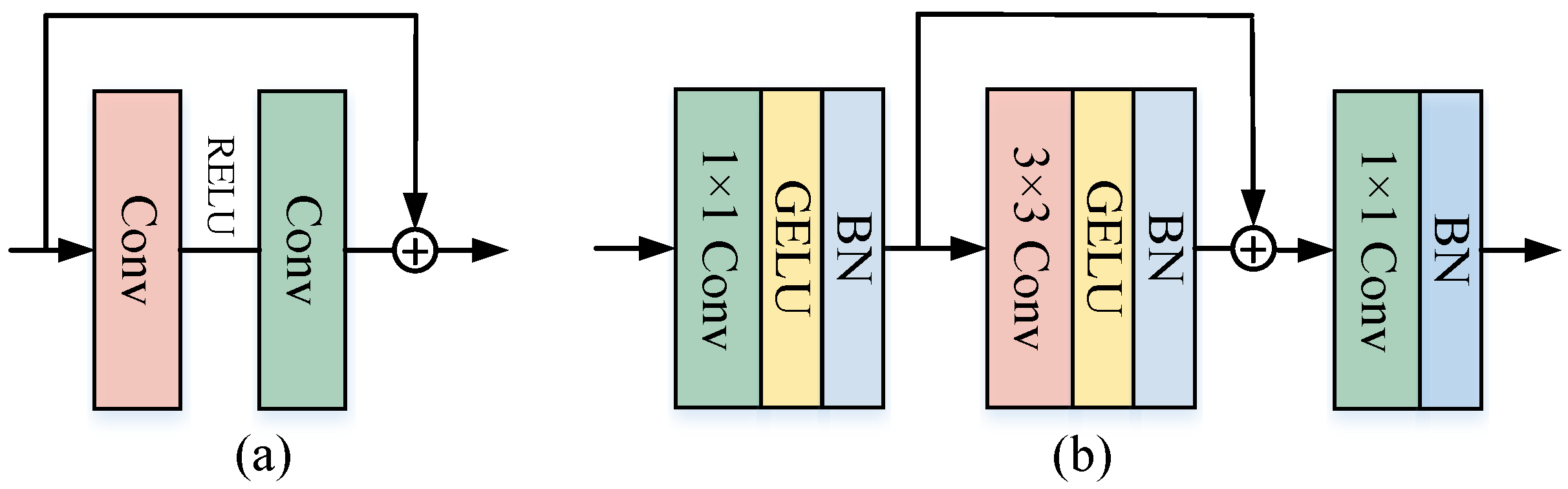
where GELU represents the activation function. $W_1\in {\mathbb{R}}^{(d \times 4d)}$ and $W_2\in {\mathbb{R}}^{(4d \times d)}$ represent the weights of the two linear layers, respectively, and $b_1$ and $b_2$ are two bias terms. The coordination between the FFN and the self-attention layer is not sufficiently tight, so it cannot effectively utilize the global information extracted by the self-attention layer, resulting in overall performance degradation. To address this limitation, this article proposes a residual feedforward network (ResFFN) structure by incorporating residual blocks. Figure 4a displays an original residual block consisting of multiple convolutional layers and activation functions. Figure 4b shows ResFFN, which overall is similar to an inverted residual block [40]. ResFFN comprises three convolutional layers arranged sequentially, BatchNorm (BN), and the GELU activation function. Among these, the BN layer plays a crucial role in accelerating the network’s convergence speed and facilitating network training, and the three sequentially arranged convolutional layers further extract local features embedded within PolSAR images. These consist of a first 1 × 1 convolutional layer, a 3 × 3 convolutional layer, and a final 1 × 1 convolutional layer. Specifically, this module achieves better performance by altering the position of the residual connection. Assuming that $\beta$ is the input, ResFFN can be represented as given in Equations (13) and ():

$$\begin{array}{c}\hfill ResFFN\left(\beta \right)=\mathrm{Conv}\left(\phi \right(\mathrm{Conv}\left(\beta \right)\left)\right),\end{array}$$

(13)

$$\begin{array}{c}\hfill \phi \left(\beta \right)=\mathrm{Conv}\left(\beta \right)+\beta .\end{array}$$

(14)

where ResFFN stands for the residual feedforward network and Conv represents a convolution operation; a 3 × 3 convolution is used to extract local information. The introduction of residual blocks not only effectively promotes the interaction between local and global information but also improves the cross-layer propagation of gradients, which is conducive to obtaining better results in experiments.

3. Experimental Results and Analysis

This section first outlines the datasets employed in the experiments as well as the experimental configurations. It then elaborates on the objective evaluation metrics used to measure the experimental results. Subsequently, an ablation study is conducted on the various modules of the proposed method across three different datasets. Finally, the results of the comparative experiments are presented and analyzed.

3.1. PolSAR Datasets and Experimental Setup

The following datasets were used in the experiments:

1.

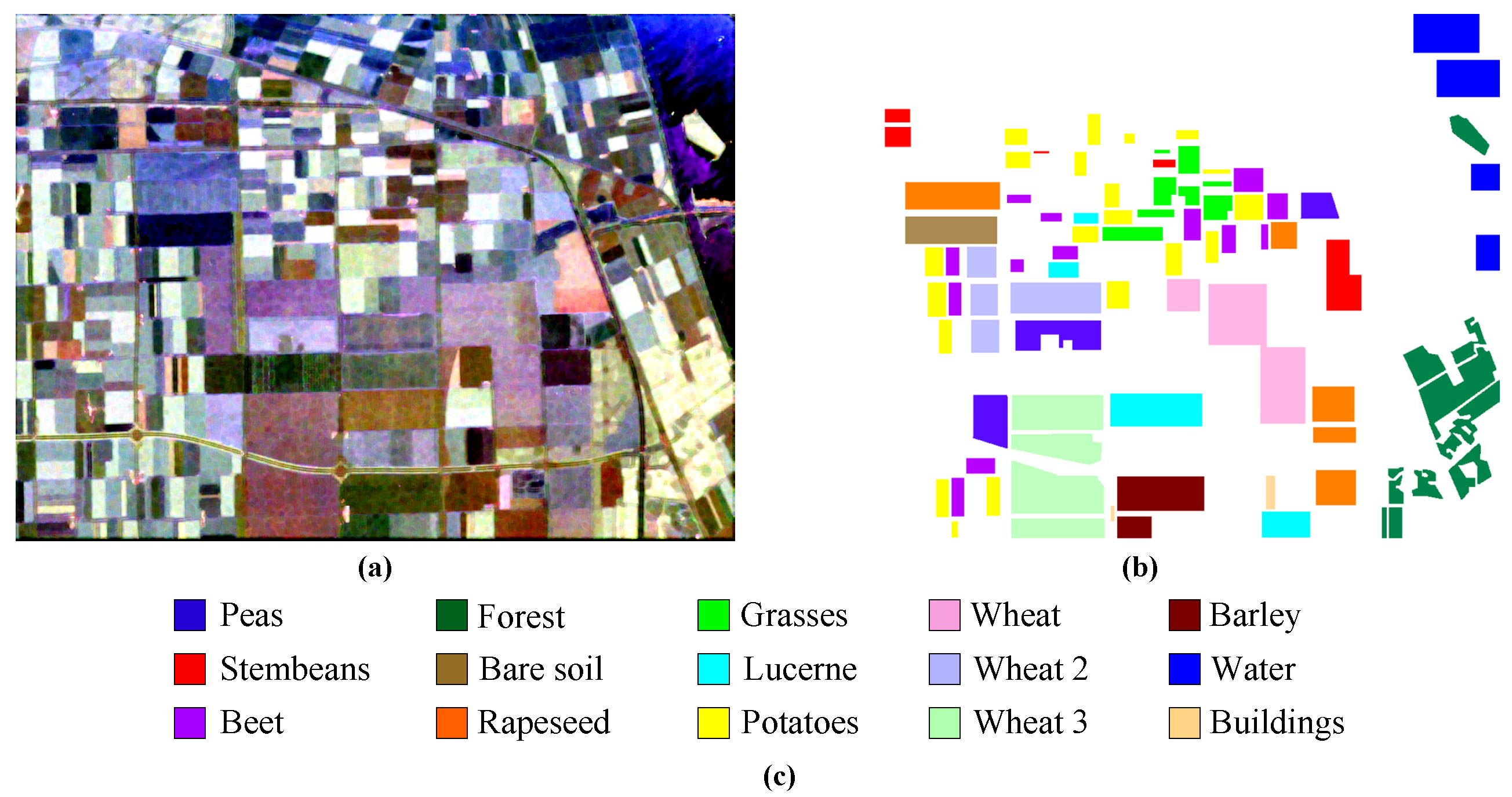
AIRSAR Flevoland. This dataset contains L-band images obtained by the AIRSAR platform, with a size of 750 × 1024 pixels, consisting of 15 different feature categories [41], each of which is identified by a unique color. Figure 5a shows a Pauli RGB image of the selected scene, Figure 5b shows a ground-truth map containing 167,712 annotated pixels, and Figure 5c shows a legend of the feature categories.

Figure 5. Image from the AIRSAR Flevoland dataset. (a) Pauli RGB image. (b) Ground-truth map. (c) Legend of feature categories.

Figure 5. Image from the AIRSAR Flevoland dataset. (a) Pauli RGB image. (b) Ground-truth map. (c) Legend of feature categories.

2.

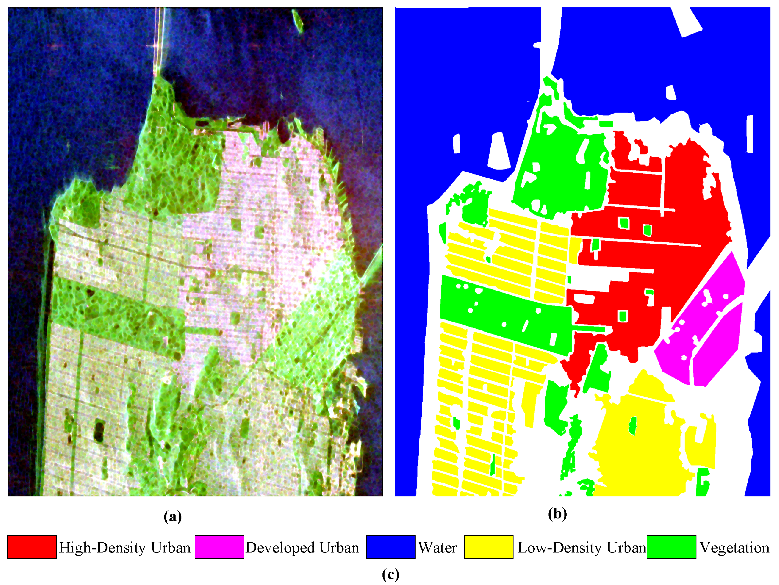
RADARSAT-2 San Francisco. This dataset contains C-band images of San Francisco obtained by the RADARSAT-2 satellite, with a size of 1380 × 1800, and mainly includes five land-cover types [42]. Figure 6a shows a Pauli RGB image of the selected scene, Figure 6b shows a ground-truth map composed of 1,804,087 annotated pixels, and Figure 6c shows a legend of the land-cover types.

Figure 6. Image from the RADARSAT-2 San Francisco dataset. (a) Pauli RGB image. (b) Ground-truth map. (c) Legend of land-cover types.

Figure 6. Image from the RADARSAT-2 San Francisco dataset. (a) Pauli RGB image. (b) Ground-truth map. (c) Legend of land-cover types.

3.

RADARSAT-2 Xi’an dataset. This dataset contains fully polarized C-band images obtained from the western part of Xianyang City and the Weihe River region in Shaanxi Province, China, using the RADARSAT-2 satellite. The images have a size of 512 × 512 and cover three typical terrain types. Figure 7a shows a Pauli RGB image of the selected scene, Figure 7b shows a ground-truth map consisting of 237,416 annotated pixels, and Figure 7c shows a legend of the terrain types.

Figure 7. Image from the RADARSAT-2 Xi’an dataset. (a) Pauli RGB image. (b) Ground-truth map. (c) Legend of terrain types.

Figure 7. Image from the RADARSAT-2 Xi’an dataset. (a) Pauli RGB image. (b) Ground-truth map. (c) Legend of terrain types.

All experiments were conducted using PyTorch version 1.11.0 and CUDA version 11.3 of the PyTorch GPU deep learning framework on NVIDIA GeForce RTX 3090 high-performance servers. The following section provides a detailed introduction to the experimental setup. Since the model used in this experiment is based on ViT, the image formats are used as input. First, a neighborhood with a size of 14 × 14 was extracted from each pixel as the initial input, and the input space size p was set to 15. The specific parameter configurations for the components of the proposed model are shown in

Table 1. Parameter configurations for the three components of the proposed model.

Module	Parameter Configuration
CCLP	Channel-Wise Convolution	Local Residual Connection
	Conv@ [3 × 3, 5 × 5, 7 × 7]	Conv@ 3 × 3, ⊕
DTA	Chunk-Wise Attention	Point-Wise Attention
	chunk_size = 3, depth = 1	chunk_size = 3, depth = 1
	Attention: 3 × (64 × 64)	Attention: 3 × (64 × 64)
ResFFN	ffn_ratio = 4
	Conv@ 1 × 1
	Conv@ 3 × 3, ⊕
	Conv@ 1 × 1

; in the table, ⊕ denotes the residual connections.

In addition, different datasets were trained with different amounts of labeled data in the experiments. Each category in the Flevoland dataset was trained using 300 labeled data points, accounting for 2.68%. Each category in the San Francisco dataset was trained using 900 labeled data points, representing 0.25%. In the Xi’an dataset, each category was trained using 400 labeled data points, accounting for 0.50% of the total. Selecting training data by category can effectively alleviate the problem of sample imbalance.

During the training process, a 5-fold cross-validation method was used; each fold contained 100 training epochs, and the batch size was 256. The learning rate was automatically adjusted using the Adam optimizer, with the initial learning rate set to $1\times {10}^{-4}$, and the cross-entropy loss was used as the loss function. Assuming that $y_l^m$ represents the reference label and ${\widehat{y}}_l^m$ represents the predicted label, the cross-entropy loss $Los{s}_{CE}$ can be expressed as given in Equation (15):

$$\begin{array}{c}\hfill Los{s}_{CE}=-\sum _{m=1}^M\sum _{l=1}^L{y}_l^{m}log\left({\widehat{y}}_l^m\right).\end{array}$$

(15)

Finally, the fold with the highest overall accuracy in the 5-fold model was selected for the prediction of the subsequent results.

3.2. Objective Evaluation Metrics

The experiment used overall accuracy (OA), average accuracy (AA), and the Kappa coefficient (Kappa) as evaluation metrics to evaluate the classification performance of the model. OA is an overall metric that assesses the performance of a classification model. It measures the proportion of correctly predicted samples to the total number of samples. Its expression is shown in Equation (16):

$$\begin{array}{c}\hfill \mathrm{OA}={\displaystyle \frac{TP+TN}{TP+FN+FP+TN}},\end{array}$$

(16)

where TP stands for true positives, FN denotes false negatives, FP represents false positives, and TN denotes true negatives. AA stands for average accuracy, which represents the mean accuracy across different categories. It reflects the model’s balanced performance across classes, as expressed in Equations (17) and (18):

$$\begin{array}{c}\hfill \mathrm{AA}={\displaystyle \frac{\sum {\mathrm{Recall}}_i}{N_i}},\end{array}$$

(17)

$$\begin{array}{c}\hfill \mathrm{Recall}={\displaystyle \frac{TP}{TP+FN}},\end{array}$$

(18)

Recall is the ratio of correctly classified positive samples to the total number of actual positive samples; i denotes the category, and $N_i$ indicates the number of categories. The Kappa coefficient is a statistical metric used to assess the agreement between predicted and true classifications, adjusted for chance agreement. It more accurately reflects performance than OA alone. The Kappa value ranges from −1 to +1, with higher values indicating stronger agreement. Its expression is given in Equation (19):

$$\begin{array}{c}\hfill \mathrm{Kappa}={\displaystyle \frac{p_0-p_e}{1-p_e}},\end{array}$$

(19)

where $p_0$ denotes the overall classification accuracy; $a_1$, $a_2$, . . . , $a_c$ denote the number of true samples per class; $b_1$, $b_2$, . . . , $b_c$ denote the number of predicted samples per class; and n denotes the total number of samples. $p_e$ is calculated as shown in Equation (20):

$$\begin{array}{c}\hfill p_e={\displaystyle \frac{a_1\times b_1+a_2\times b_2+\cdots +a_c\times b_c}{n^2}}.\end{array}$$

(20)

In summary, OA, AA, and Kappa are all important metrics for evaluating the performance of classification models. OA measures overall performance, AA assesses category-wise performance, and Kappa accounts for random agreement, thus providing a more accurate measure of consistency. In practical applications, appropriate evaluation metrics can be selected based on specific needs.

3.3. Ablation Study

To comprehensively validate the effectiveness and reliability of the proposed method, this study conducted ten ablation experiments on each of the three datasets—Flevoland, San Francisco, and Xi’an—with the average values calculated based on the experimental outcomes. Additionally, to enhance the intuitiveness of the experimental results, only OA among the three evaluation metrics was selected to assess classification performance during the ablation experiments.

Table 2. Results of the ablation study on the three datasets.

Scheme	CCLP	DTA	ResFFN	OA (%)
				Flevoland	San Francisco	Xi’an
(1)				97.66	97.33	89.95
(2)	✓			+0.38 (98.04)	+0.14 (97.47)	+0.36 (90.31)
(3)		✓		+0.63 (98.29)	+0.17 (97.50)	+0.77 (90.72)
(4)			✓	+0.26 (97.92)	+0.09 (97.42)	+0.12 (90.07)
(5)	✓	✓		+1.17 (98.83)	+0.25 (97.58)	+1.08 (91.03)
(6)	✓		✓	+0.91 (98.57)	+0.20 (97.53)	+0.54 (90.49)
(7)		✓	✓	+1.45 (99.11)	+0.27 (97.60)	+0.95 (90.86)
(8)	✓	✓	✓	+1.90 (99.56)	+0.31 (97.64)	+1.39 (91.34)

presents the detailed results of the ablation experiments. Values marked in blue indicate an increase in OA compared to the baseline model, with the corresponding OA values shown in parentheses. Each experimental scheme has been numbered to facilitate an in-depth analysis of the results in subsequent steps.

Scheme (1) in Table 2 adopted ViT as the baseline model, and the experimental results indicate that ViT exhibited relatively impressive classification accuracy across the three datasets. Scheme (2) integrated the CCLP module into ViT, and the findings revealed that the CCLP module facilitated the extraction of local information from PolSAR images, leading to enhanced classification performance. Specifically, the OA across the three datasets increased by 0.38%, 0.14%, and 0.36%, respectively. Scheme (3) combined the DTA module with ViT, resulting in OA improvements of 0.63%, 0.17%, and 0.77% on the three datasets, respectively. This indicates that the DTA module improves the classification accuracy of the model and promotes the interaction and fusion of local and global information in PolSAR images. Scheme (4) showcases the efficacy of the ResFFN module, with OA enhancements of 0.26%, 0.09%, and 0.12%, respectively, compared to the baseline model. When utilized alone, the ResFFN module exhibited a relatively modest improvement in classification accuracy compared to the CCLP and DTA modules. Scheme (5) integrated the CCLP and DTA modules, yielding OA improvements of 1.17%, 0.25%, and 1.08%, respectively, across the three datasets when benchmarked against the baseline model. Scheme (6) paired CCLP with the ResFFN module, revealing performance enhancements, with OA increases of 0.91%, 0.2%, and 0.54%, respectively, compared to the baseline model. Scheme (7) combined DTA with the ResFFN module, resulting in OA improvements of 1.45%, 0.27%, and 0.95%, respectively, across the three datasets compared to the baseline model. Furthermore, the outcomes of Schemes (5) to (7) demonstrate that combining the CCLP, DTA, and ResFFN modules yielded higher classification accuracy across all three datasets than when each module was used in isolation. Scheme (8) represents the proposed methodology, where the synergistic action of the three modules significantly elevated the overall classification performance of the model. Compared to the baseline model, the OA of the three datasets increased by 1.9%, 0.31%, and 1.39%, respectively.

In summary, the results of the ablation experiments have effectively validated the efficacy of the CCLP, DTA, and ResFFN modules. These modules excel in facilitating the interaction between local and global information within PolSAR images, thereby significantly enhancing the classification accuracy of the datasets. The results of the ablation experiments offer further validation for the feasibility of employing the proposed method in the PolSAR image classification task.

3.4. Comparative Experimental Results and Analysis

In this section, the classification performance of the proposed method is evaluated using the three datasets mentioned previously, and the objective evaluation metrics and subjective judgment are provided based on the experimental results of each dataset. All methods adopted identical training settings (the cross-entropy loss function, the Adam optimizer, a learning rate of $1\times {10}^{-4}$, a weight decay of $1\times {10}^{-3}$, and a batch size of 256). Seven advanced models were selected for comparison, encompassing CNN-based classification methods (CV-3D-CNN [43] and ResNet-34 [44]), ViT-based methods (SViT [28] and CrossViT [45]), and CNN–ViT fusion methods (CCT [46], MCPT [29], and MGFFT [30]). The detailed results of the comparative experiments on the three datasets are presented in Table 3, Table 4 and Table 5. In the tables, values in bold indicate optimal classification accuracy, while those underlined denote sub-optimal classification accuracy. The prediction results of each method are visually depicted in Figure 8, Figure 9 and Figure 10. Given that the experiment adopted a 5-fold cross-validation approach, the objective evaluation metrics, including OA, AA, and the Kappa coefficient, display the mean values and standard deviations obtained from the 5-fold cross-validation. Subjective judgment uses corresponding colors to illustrate the classification results of the predicted image. The combination of the objective evaluation metrics and subjective judgment makes the experimental results clearer and more intuitive.

3.4.1. Analysis of the Experimental Results on the AIRSAR Flevoland Dataset

The experimental results of the comparative experiment on the Flevoland dataset are shown in Table 3, and the predicted results of all pixels are shown in Figure 8. The OA, AA, and Kappa values for CV-3D-CNN were at an intermediate level compared to the other methods. Although CV-3D-CNN performed the best in classifying Forests and Peas, it performed poorly in classifying Barley. ResNet-34, a deep residual network, performed well in classifying Barely, Wheat 2, and Stem Beans, but it had a large standard deviation across all three evaluation metrics, indicating poor stability. SViT represents the first application of ViT in PolSAR image classification, and its three evaluation metrics were at an intermediate level, similar to those of CV-3D-CNN. CCT, a model that combines a CNN and ViT, achieved relatively average classification performance across the 15 categories, indicating that it was not competitive. CrossViT, an improved variant of the ViT due to its attention mechanism, performed poorly in the PolSAR image classification task, especially in classifying Rapeseed, with an accuracy of only 82.95%. MCPT and MGFFT, which both integrate CNNs and ViTs, achieved classification performance that was second only to that of the proposed method. MGFFT achieved the best classification accuracy in the Stem Beans and Buildings categories. Although its three evaluation metrics were second only to those of the proposed method, its standard deviation indicated that its performance was not as stable as that of the proposed method. The proposed method achieved the highest OA values on the Flevoland dataset, with a low standard deviation, stable performance, and the fastest training and prediction times. In addition, the Buildings category, which had the fewest labeled samples, was also classified well. This indicates that the proposed method can maintain good classification performance even when only a small number of labeled samples are available.

Table 3. Objective evaluation metrics for eight methods on the AIRSAR Flevoland dataset.

	CV-3D-CNN [43]	ResNet-34 [44]	SViT [28]	CCT [46]	CrossViT [45]	MCPT [29]	MGFFT [30]	Proposed Method
Water	0.9932 ± 0.0073	0.9940 ± 0.0218	0.8977 ± 0.0010	0.9322 ± 0.0090	0.9647 ± 0.0073	0.9898 ± 0.0150	0.9989 ± 0.0021	0.9999 ± 0.0042
Forest	0.9993 ± 0.0108	0.9958 ± 0.0530	0.9901 ± 0.0430	0.9886 ± 0.0620	0.9833 ± 0.0018	0.9927 ± 0.0116	0.9914 ± 0.0106	0.9898 ± 0.0013
Lucerne	0.9839 ± 0.0069	0.9852 ± 0.0384	0.9885 ± 0.0015	0.9935 ± 0.0005	0.9848 ± 0.0004	0.9872 ± 0.0118	0.9941 ± 0.0051	0.9998 ± 0.0019
Grass	0.9792 ± 0.0251	0.8393 ± 0.0086	0.9796 ± 0.0007	0.9610 ± 0.0074	0.9282 ± 0.0015	0.9620 ± 0.0042	0.9781 ± 0.0091	0.9959 ± 0.0030
Peas	0.9990 ± 0.0007	0.9958 ± 0.0172	0.9886 ± 0.0042	0.9781 ± 0.0003	0.9796 ± 0.0081	0.9954 ± 0.0106	0.9984 ± 0.0012	0.9988 ± 0.0053
Barley	0.8964 ± 0.1045	0.9999 ± 0.0077	0.9976 ± 0.0090	0.9879 ± 0.0020	0.9984 ± 0.0061	0.9943 ± 0.0022	0.9963 ± 0.0022	0.9993 ± 0.0018
Bare Soil	0.9945 ± 0.0078	0.9937 ± 0.0350	0.9922 ± 0.0033	0.9986 ± 0.0102	0.9988 ± 0.0012	0.9988 ± 0.0096	0.9968 ± 0.0015	0.9999 ± 0.0061
Beet	0.9808 ± 0.0107	0.9862 ± 0.0091	0.9845 ± 0.0005	0.9786 ± 0.0018	0.9435 ± 0.0076	0.9851 ± 0.0116	0.9856 ± 0.0103	0.9971 ± 0.0020
Wheat 2	0.9759 ± 0.0290	0.9900 ± 0.0132	0.9802 ± 0.0082	0.9513 ± 0.0026	0.9694 ± 0.0025	0.9796 ± 0.0448	0.9760 ± 0.0322	0.9846 ± 0.0014
Wheat 3	0.9913 ± 0.0095	0.9926 ± 0.0066	0.9957 ± 0.0063	0.9804 ± 0.0046	0.9963 ± 0.0032	0.9857 ± 0.0014	0.9948 ± 0.0011	0.9992 ± 0.0011
Stem Beans	0.9907 ± 0.0004	0.9998 ± 0.0073	0.9860 ± 0.0017	0.9961 ± 0.0040	0.8395 ± 0.0406	0.9888 ± 0.0105	0.9998 ± 0.0031	0.9996 ± 0.0001
Rapeseed	0.9484 ± 0.0552	0.8937 ± 0.0094	0.9629 ± 0.0041	0.9528 ± 0.0076	0.8295 ± 0.0112	0.9461 ± 0.0088	0.9527 ± 0.0078	0.9977 ± 0.0006
Wheat	0.9871 ± 0.0030	0.9670 ± 0.0054	0.9603 ± 0.0005	0.9542 ± 0.0005	0.9442 ± 0.0014	0.9863 ± 0.0170	0.9882 ± 0.0033	0.9923 ± 0.0018
Buildings	0.9822 ± 0.0249	0.9946 ± 0.0703	0.9973 ± 0.0241	0.9973 ± 0.0062	0.9415 ± 0.0006	0.9959 ± 0.0094	0.9993 ± 0.0006	0.9971 ± 0.0003
Potatoes	0.9764 ± 0.0333	0.9892 ± 0.0106	0.9864 ± 0.0030	0.9879 ± 0.0014	0.8936 ± 0.0044	0.9949 ± 0.0027	0.9836 ± 0.0001	0.9972 ± 0.0014
AA	0.9784 ± 0.0153	0.9744 ± 0.0647	0.9792 ± 0.0705	0.9759 ± 0.0052	0.9464 ± 0.0160	0.9855 ± 0.0044	0.9889 ± 0.0034	0.9964 ± 0.0017
Kappa	0.9792 ± 0.0169	0.9732 ± 0.0934	0.9746 ± 0.0027	0.9703 ± 0.0017	0.9436 ± 0.0275	0.9832 ± 0.0060	0.9876 ± 0.0048	0.9951 ± 0.0023
OA	0.9775 ± 0.0054	0.9754 ± 0.0336	0.9767 ± 0.0056	0.9727 ± 0.0303	0.9482 ± 0.0034	0.9846 ± 0.0062	0.9864 ± 0.0048	0.9956 ± 0.0014

Table 3. Objective evaluation metrics for eight methods on the AIRSAR Flevoland dataset.

	CV-3D-CNN [43]	ResNet-34 [44]	SViT [28]	CCT [46]	CrossViT [45]	MCPT [29]	MGFFT [30]	Proposed Method
Water	0.9932 ± 0.0073	0.9940 ± 0.0218	0.8977 ± 0.0010	0.9322 ± 0.0090	0.9647 ± 0.0073	0.9898 ± 0.0150	0.9989 ± 0.0021	0.9999 ± 0.0042
Forest	0.9993 ± 0.0108	0.9958 ± 0.0530	0.9901 ± 0.0430	0.9886 ± 0.0620	0.9833 ± 0.0018	0.9927 ± 0.0116	0.9914 ± 0.0106	0.9898 ± 0.0013
Lucerne	0.9839 ± 0.0069	0.9852 ± 0.0384	0.9885 ± 0.0015	0.9935 ± 0.0005	0.9848 ± 0.0004	0.9872 ± 0.0118	0.9941 ± 0.0051	0.9998 ± 0.0019
Grass	0.9792 ± 0.0251	0.8393 ± 0.0086	0.9796 ± 0.0007	0.9610 ± 0.0074	0.9282 ± 0.0015	0.9620 ± 0.0042	0.9781 ± 0.0091	0.9959 ± 0.0030
Peas	0.9990 ± 0.0007	0.9958 ± 0.0172	0.9886 ± 0.0042	0.9781 ± 0.0003	0.9796 ± 0.0081	0.9954 ± 0.0106	0.9984 ± 0.0012	0.9988 ± 0.0053
Barley	0.8964 ± 0.1045	0.9999 ± 0.0077	0.9976 ± 0.0090	0.9879 ± 0.0020	0.9984 ± 0.0061	0.9943 ± 0.0022	0.9963 ± 0.0022	0.9993 ± 0.0018
Bare Soil	0.9945 ± 0.0078	0.9937 ± 0.0350	0.9922 ± 0.0033	0.9986 ± 0.0102	0.9988 ± 0.0012	0.9988 ± 0.0096	0.9968 ± 0.0015	0.9999 ± 0.0061
Beet	0.9808 ± 0.0107	0.9862 ± 0.0091	0.9845 ± 0.0005	0.9786 ± 0.0018	0.9435 ± 0.0076	0.9851 ± 0.0116	0.9856 ± 0.0103	0.9971 ± 0.0020
Wheat 2	0.9759 ± 0.0290	0.9900 ± 0.0132	0.9802 ± 0.0082	0.9513 ± 0.0026	0.9694 ± 0.0025	0.9796 ± 0.0448	0.9760 ± 0.0322	0.9846 ± 0.0014
Wheat 3	0.9913 ± 0.0095	0.9926 ± 0.0066	0.9957 ± 0.0063	0.9804 ± 0.0046	0.9963 ± 0.0032	0.9857 ± 0.0014	0.9948 ± 0.0011	0.9992 ± 0.0011
Stem Beans	0.9907 ± 0.0004	0.9998 ± 0.0073	0.9860 ± 0.0017	0.9961 ± 0.0040	0.8395 ± 0.0406	0.9888 ± 0.0105	0.9998 ± 0.0031	0.9996 ± 0.0001
Rapeseed	0.9484 ± 0.0552	0.8937 ± 0.0094	0.9629 ± 0.0041	0.9528 ± 0.0076	0.8295 ± 0.0112	0.9461 ± 0.0088	0.9527 ± 0.0078	0.9977 ± 0.0006
Wheat	0.9871 ± 0.0030	0.9670 ± 0.0054	0.9603 ± 0.0005	0.9542 ± 0.0005	0.9442 ± 0.0014	0.9863 ± 0.0170	0.9882 ± 0.0033	0.9923 ± 0.0018
Buildings	0.9822 ± 0.0249	0.9946 ± 0.0703	0.9973 ± 0.0241	0.9973 ± 0.0062	0.9415 ± 0.0006	0.9959 ± 0.0094	0.9993 ± 0.0006	0.9971 ± 0.0003
Potatoes	0.9764 ± 0.0333	0.9892 ± 0.0106	0.9864 ± 0.0030	0.9879 ± 0.0014	0.8936 ± 0.0044	0.9949 ± 0.0027	0.9836 ± 0.0001	0.9972 ± 0.0014
AA	0.9784 ± 0.0153	0.9744 ± 0.0647	0.9792 ± 0.0705	0.9759 ± 0.0052	0.9464 ± 0.0160	0.9855 ± 0.0044	0.9889 ± 0.0034	0.9964 ± 0.0017
Kappa	0.9792 ± 0.0169	0.9732 ± 0.0934	0.9746 ± 0.0027	0.9703 ± 0.0017	0.9436 ± 0.0275	0.9832 ± 0.0060	0.9876 ± 0.0048	0.9951 ± 0.0023
OA	0.9775 ± 0.0054	0.9754 ± 0.0336	0.9767 ± 0.0056	0.9727 ± 0.0303	0.9482 ± 0.0034	0.9846 ± 0.0062	0.9864 ± 0.0048	0.9956 ± 0.0014

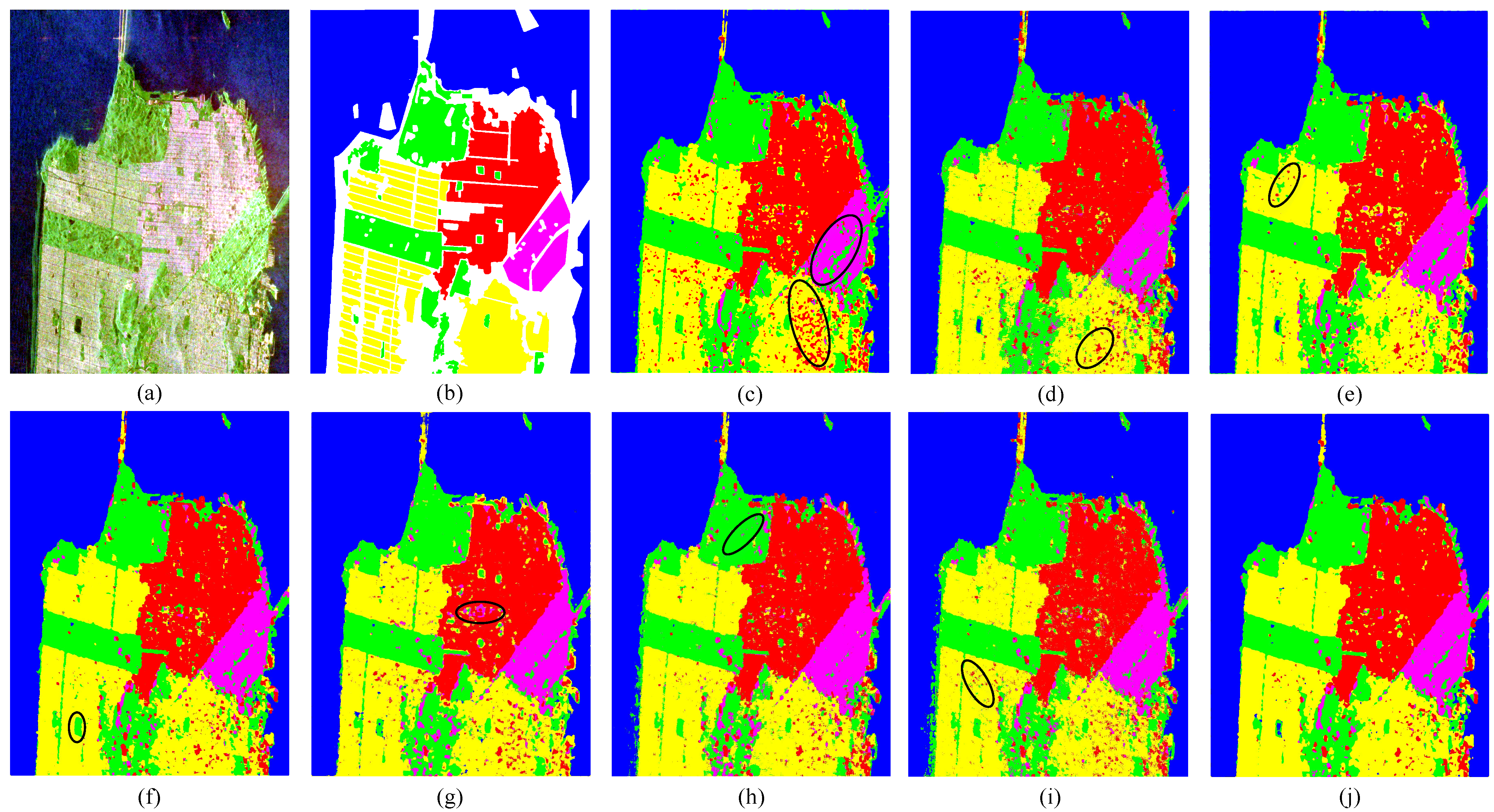
Figure 8 illustrates the prediction results of the different classification methods on an image from the Flevoland dataset. Figure 8a shows the Pauli RGB image, and Figure 8b shows the corresponding ground-truth map. The areas enclosed by black ellipses indicate regions with classification errors. Figure 8c depicts the classification result of CV-3D-CNN, where significant classification errors are visible in the marked region. Moreover, there are numerous scattered misclassified pixels in the Forest area in the lower-right part of the image. As shown in Figure 8d, ResNet-34 performs well in some labeled data regions but fails to accurately classify Rapeseed within the black ellipse. Figure 8e displays the classification result of SViT, which also exhibits classification errors in the same region as CV-3D-CNN, as well as noticeable misclassification in the Water area in the upper-right part of the image. Figure 8f shows the prediction result of CCT, where a substantial amount of speckled noise can be seen in the black ellipse in the lower-right part of the image, and the Water area in the upper-right part cannot be clearly distinguished. From Figure 8g, it can be inferred that CrossViT exhibits poor edge classification performance in the red Stem Beans area. Classification errors can also be seen in the black ellipse. Figure 8h presents the classification result of MCPT. Although its overall performance is superior to that of the other comparative methods, there are still obvious classification errors visible in the black ellipse in the lower part of the image. Figure 8i shows the classification result of MGFFT, where a relatively large amount of speckle noise can be seen in the black ellipse in the upper-right part of the image. Figure 8j shows the classification result of the proposed method. The boundaries between the Stem Beans and Water areas on the right side are clearly defined. The scattering characteristics of ground objects in PolSAR images are similar (such as Bare Soil and Wheat), which contributes to aleatory uncertainty. Meanwhile, the reliance of the model on local features may cause epistemic uncertainty. The MGFFT method reduces uncertainty through multiscale feature fusion and achieves excellent performance in classifying Stem Beans and Buildings. However, its Kappa coefficient has a higher standard deviation than that of the proposed method, indicating lower stability. The proposed method achieves the same accuracy as MGFFT in classifying Buildings (with the fewest labeled samples) but achieves higher OA values and a significantly lower standard deviation. In addition, its classification of edge regions (such as the boundary between Stem Beans and Water) is clearer, and there is less noise, indicating a stronger ability to balance local and global features. Compared with the other methods, the proposed method achieves better prediction accuracy and stronger stability.

Figure 8. Classification results for the image from the Flevoland dataset. (a) Pauli RGB image. (b) Ground-truth map. (c) CV-3D-CNN. (d) ResNet-34. (e) SViT. (f) CCT. (g) CrossViT. (h) MCPT. (i) MGFFT. (j) Proposed method.

Figure 8. Classification results for the image from the Flevoland dataset. (a) Pauli RGB image. (b) Ground-truth map. (c) CV-3D-CNN. (d) ResNet-34. (e) SViT. (f) CCT. (g) CrossViT. (h) MCPT. (i) MGFFT. (j) Proposed method.

3.4.2. Analysis of the Experimental Results on the San Francisco Dataset

The prediction results of the models presented in Table 4 show that CV-3D-CNN performed poorly on the San Francisco dataset compared to the other methods, especially for the Developed category, with an accuracy of only 87.63%. The ResNet-34 model achieved moderate results across all three evaluation metrics, second only to the ViT-based method, but it performed better in classifying Vegetables and High-Density Urban areas. SViT achieved the highest AA on this dataset. Its high standard deviation indicates stable classification performance, but its long training time demonstrates limited competitiveness. CCT achieved the highest classification accuracy for the Water category, but its overall performance was hindered by longer training and prediction times. CrossViT, a variant of ViT, showed average overall performance; however, it performed well in classifying Water areas and was second only to CCT. The OA value of the MCPT method was second only to that of SViT, and it performed well in classifying Developed areas. MGFFT, a method that combines CNN and ViT architectures, performed poorly on the San Francisco dataset, possibly because it did not successfully balance the characteristics of these architectures. The proposed method not only achieved the highest classification accuracy for Low-Density Urban areas but also attained the best values for both overall accuracy (OA) and the Kappa coefficient. This indicates that the proposed method holds an advantage over the other methods in terms of feature learning.

Table 4. Objective evaluation metrics for eight methods on the RADARSAT-2 San Francisco dataset.

	CV-3D-CNN [43]	ResNet-34 [44]	SViT [28]	CCT [46]	CrossViT [45]	MCPT [29]	MGFFT [30]	Proposed Method
Water	0.9988 ± 0.0064	0.9999 ± 0.0055	0.9969 ± 0.0004	0.9999 ± 0.0001	0.9994 ± 0.0035	0.9994 ± 0.0041	0.9992 ± 0.0008	0.9991 ± 0.0014
Vegetation	0.8953 ± 0.0066	0.9447 ± 0.0103	0.9318 ± 0.0072	0.9352 ± 0.0002	0.9329 ± 0.0012	0.9026 ± 0.0013	0.9170 ± 0.0002	0.9375 ± 0.0003
High-Density Urban	0.9509 ± 0.0013	0.9761 ± 0.0049	0.9746 ± 0.0032	0.9598 ± 0.0010	0.9494 ± 0.0038	0.9661 ± 0.0020	0.9466 ± 0.0037	0.9588 ± 0.0004
Developed	0.8763 ± 0.0027	0.9443 ± 0.0019	0.9644 ± 0.0010	0.9460 ± 0.0007	0.9515 ± 0.0033	0.9792 ± 0.0045	0.9554 ± 0.0013	0.9579 ± 0.0023
Low-Density Urban	0.9054 ± 0.0035	0.9242 ± 0.0024	0.9453 ± 0.0008	0.9453 ± 0.0001	0.9254 ± 0.0012	0.9591 ± 0.0023	0.9287 ± 0.0034	0.9663 ± 0.0001
AA	0.9253 ± 0.0002	0.9578 ± 0.0062	0.9626 ± 0.0076	0.9572 ± 0.0026	0.9517 ± 0.0070	0.9613 ± 0.0006	0.9494 ± 0.0028	0.9612 ± 0.0040
Kappa	0.9298 ± 0.0049	0.9593 ± 0.0145	0.9617 ± 0.0055	0.9599 ± 0.0004	0.9515 ± 0.0014	0.9607 ± 0.0006	0.9645 ± 0.0009	0.9661 ± 0.0007
OA	0.9512 ± 0.0007	0.9717 ± 0.0022	0.9733 ± 0.0118	0.9721 ± 0.0037	0.9663 ± 0.0093	0.9727 ± 0.0008	0.9490 ± 0.0014	0.9764 ± 0.0001

Table 4. Objective evaluation metrics for eight methods on the RADARSAT-2 San Francisco dataset.

	CV-3D-CNN [43]	ResNet-34 [44]	SViT [28]	CCT [46]	CrossViT [45]	MCPT [29]	MGFFT [30]	Proposed Method
Water	0.9988 ± 0.0064	0.9999 ± 0.0055	0.9969 ± 0.0004	0.9999 ± 0.0001	0.9994 ± 0.0035	0.9994 ± 0.0041	0.9992 ± 0.0008	0.9991 ± 0.0014
Vegetation	0.8953 ± 0.0066	0.9447 ± 0.0103	0.9318 ± 0.0072	0.9352 ± 0.0002	0.9329 ± 0.0012	0.9026 ± 0.0013	0.9170 ± 0.0002	0.9375 ± 0.0003
High-Density Urban	0.9509 ± 0.0013	0.9761 ± 0.0049	0.9746 ± 0.0032	0.9598 ± 0.0010	0.9494 ± 0.0038	0.9661 ± 0.0020	0.9466 ± 0.0037	0.9588 ± 0.0004
Developed	0.8763 ± 0.0027	0.9443 ± 0.0019	0.9644 ± 0.0010	0.9460 ± 0.0007	0.9515 ± 0.0033	0.9792 ± 0.0045	0.9554 ± 0.0013	0.9579 ± 0.0023
Low-Density Urban	0.9054 ± 0.0035	0.9242 ± 0.0024	0.9453 ± 0.0008	0.9453 ± 0.0001	0.9254 ± 0.0012	0.9591 ± 0.0023	0.9287 ± 0.0034	0.9663 ± 0.0001
AA	0.9253 ± 0.0002	0.9578 ± 0.0062	0.9626 ± 0.0076	0.9572 ± 0.0026	0.9517 ± 0.0070	0.9613 ± 0.0006	0.9494 ± 0.0028	0.9612 ± 0.0040
Kappa	0.9298 ± 0.0049	0.9593 ± 0.0145	0.9617 ± 0.0055	0.9599 ± 0.0004	0.9515 ± 0.0014	0.9607 ± 0.0006	0.9645 ± 0.0009	0.9661 ± 0.0007
OA	0.9512 ± 0.0007	0.9717 ± 0.0022	0.9733 ± 0.0118	0.9721 ± 0.0037	0.9663 ± 0.0093	0.9727 ± 0.0008	0.9490 ± 0.0014	0.9764 ± 0.0001

Figure 9 displays the prediction outcomes of the various classification methods on an image from the San Francisco dataset. Figure 9a shows the Pauli RGB image, and Figure 9b shows the corresponding ground-truth map. The areas enclosed by black ellipses indicate regions where classification errors occurred. Figure 9c illustrates the prediction result of CV-3D-CNN. Visually, it is apparent that there are numerous scattered pixels and noise within the black ellipse. Figure 9d depicts the classification result of ResNet-34. In the yellow area within the black elliptical region in the lower-right corner, which represents the Low-Density Urban category, significant classification errors are evident. In Figure 9e, in the yellow area within the black ellipse, there is a substantial amount of speckle noise. This implies that SViT, while adept at extracting global information, tends to overlook local details to some degree. Although Figure 9f shows that CCT emphasizes the processing of local information, there are still considerable discrepancies between the categories within the black elliptical region and those in the Pauli image. Figure 9g not only exhibits the same issue as CCT but also reveals that CrossViT makes obvious classification errors in the red area within the black elliptical region. The yellow area contains many miscellaneous colors, and the edges are marred by a significant amount of noise. Figure 9h presents the classification result of MCPT. It is clear that there is a considerable amount of noise in the green area within the black elliptical region in the upper part of the image. Figure 9i shows the prediction result of the MGFFT method. It can be clearly seen that the edges are impure, with a multitude of scattered pixels. There are also some green scattered pixels in the yellow area within the black elliptical region. In Figure 9j, the predicted image appears relatively pure within each color-coded region and along the edges compared with the other methods. Although there are still some miscellaneous colors, they are relatively scarce. By comparing the objective evaluation metrics in Table 4 and the prediction results in Figure 9, it can be concluded that the proposed method achieves the best performance on the San Francisco dataset.

Figure 9. Classification results for the image from the San Francisco dataset. (a) Pauli RGB image. (b) Ground-truth map. (c) CV-3D-CNN. (d) ResNet-34. (e) SViT. (f) CCT. (g) CrossViT. (h) MCPT. (i) MGFFT. (j) Proposed method.

Figure 9. Classification results for the image from the San Francisco dataset. (a) Pauli RGB image. (b) Ground-truth map. (c) CV-3D-CNN. (d) ResNet-34. (e) SViT. (f) CCT. (g) CrossViT. (h) MCPT. (i) MGFFT. (j) Proposed method.

3.4.3. Analysis of the Experimental Results on the Xi’an Dataset

As shown in Table 5, the CV-3D-CNN model yielded the lowest OA, AA, and Kappa values on this dataset. Although ResNet-34’s evaluation metrics were higher than those of the CV-3D-CNN model, it still lacked competitiveness compared to the other methods. SViT achieved good results in both the Buildings category and AA. CCT, a model based on a CNN and ViT, achieved the highest classification accuracy for the Buildings category but managed a classification accuracy of only 89.83% for the Grass category. The CrossViT model achieved the highest classification accuracy in the Grass category, but its overall performance lagged behind that of the CCT model, with a large standard deviation and poor stability. The MCPT and CCT models are both based on CNNs and ViTs. Although the three evaluation metrics for the two were similar, compared to CCT, MCPT does not have the highest classification accuracy for the category. The overall classification accuracy of MGFFT was lower than that of the other two CNN- and ViT-based methods. The proposed method achieved the best classification accuracy in the Water category, as well as the highest OA, AA, and Kappa values, on this dataset, indicating that it has an advantage over the other methods in feature extraction.

Table 5. Objective evaluation metrics for eight methods on the RADARSAT-2 Xi’an dataset.

	CV-3D-CNN [43]	ResNet-34 [44]	SViT [28]	CCT [46]	CrossViT [45]	MCPT [29]	MGFFT [30]	Proposed Method
Grass	0.9474 ± 0.0027	0.9297 ± 0.0059	0.9447 ± 0.0021	0.8983 ± 0.0042	0.9479 ± 0.0015	0.9127 ± 0.3910	0.9145 ± 0.0060	0.9204 ± 0.0006
Buildings	0.9003 ± 0.0020	0.9081 ± 0.0011	0.9247 ± 0.0053	0.9259 ± 0.0004	0.9194 ± 0.0038	0.9241 ± 0.1308	0.9048 ± 0.0059	0.9095 ± 0.0009
Water	0.8573 ± 0.0051	0.8895 ± 0.0006	0.8680 ± 0.0009	0.9020 ± 0.0107	0.8572 ± 0.0004	0.8973 ± 0.0007	0.8763 ± 0.0037	0.9184 ± 0.0065
AA	0.9017 ± 0.0007	0.9091 ± 0.0036	0.9124 ± 0.0051	0.9087 ± 0.0255	0.9081 ± 0.0068	0.9113 ± 0.0068	0.9052 ± 0.0004	0.9146 ± 0.0153
Kappa	0.8162 ± 0.0060	0.8402 ± 0.0040	0.8373 ± 0.0016	0.8518 ± 0.0017	0.8272 ± 0.0067	0.8511 ± 0.0411	0.8510 ± 0.0052	0.8591 ± 0.0018
OA	0.8861 ± 0.0120	0.9021 ± 0.0008	0.8995 ± 0.0012	0.9098 ± 0.0049	0.8928 ± 0.0251	0.9091 ± 0.0076	0.8405 ± 0.0078	0.9134 ± 0.0017

Table 5. Objective evaluation metrics for eight methods on the RADARSAT-2 Xi’an dataset.

	CV-3D-CNN [43]	ResNet-34 [44]	SViT [28]	CCT [46]	CrossViT [45]	MCPT [29]	MGFFT [30]	Proposed Method
Grass	0.9474 ± 0.0027	0.9297 ± 0.0059	0.9447 ± 0.0021	0.8983 ± 0.0042	0.9479 ± 0.0015	0.9127 ± 0.3910	0.9145 ± 0.0060	0.9204 ± 0.0006
Buildings	0.9003 ± 0.0020	0.9081 ± 0.0011	0.9247 ± 0.0053	0.9259 ± 0.0004	0.9194 ± 0.0038	0.9241 ± 0.1308	0.9048 ± 0.0059	0.9095 ± 0.0009
Water	0.8573 ± 0.0051	0.8895 ± 0.0006	0.8680 ± 0.0009	0.9020 ± 0.0107	0.8572 ± 0.0004	0.8973 ± 0.0007	0.8763 ± 0.0037	0.9184 ± 0.0065
AA	0.9017 ± 0.0007	0.9091 ± 0.0036	0.9124 ± 0.0051	0.9087 ± 0.0255	0.9081 ± 0.0068	0.9113 ± 0.0068	0.9052 ± 0.0004	0.9146 ± 0.0153
Kappa	0.8162 ± 0.0060	0.8402 ± 0.0040	0.8373 ± 0.0016	0.8518 ± 0.0017	0.8272 ± 0.0067	0.8511 ± 0.0411	0.8510 ± 0.0052	0.8591 ± 0.0018
OA	0.8861 ± 0.0120	0.9021 ± 0.0008	0.8995 ± 0.0012	0.9098 ± 0.0049	0.8928 ± 0.0251	0.9091 ± 0.0076	0.8405 ± 0.0078	0.9134 ± 0.0017

Figure 10 presents the predictive outcomes of the various classification methodologies on an image from the Xi’an dataset. Figure 10a shows the Pauli RGB image, and Figure 10b depicts the corresponding ground-truth map. The areas within the white ellipses denote regions where classification discrepancies occurred. Figure 10c illustrates the prediction result of CV-3D-CNN. In comparison with the ground-truth map, it is evident that the Water category in the lower-left corner was not adequately distinguished, and the Buildings area within the white elliptical region was inaccurately classified. Figure 10d displays the prediction result of ResNet-34. A significant amount of noise and speckles can be observed within the white elliptical region. When juxtaposed with the objective evaluation metrics, it becomes apparent that the ResNet-34 model is ill-suited for this classification task. In Figure 10e, it can be seen that SViT overlooked the Grass category within the upper white elliptical region and failed to accurately classify Buildings in the lower-left white elliptical region. Figure 10f reveals that CCT commits the same classification errors as SViT. This is predominantly because CCT has a restricted capability to enable effective interaction between local and global information. Figure 10g presents the prediction result of the CrossViT model. It is apparent that in the lower-left part of the prediction, the Buildings category within the white elliptical region is inaccurately classified. Moreover, there is a classification error for the Water category within the white elliptical region in the lower-right corner, which is in line with the results of the objective evaluation metrics. Figure 10h depicts the classification result of MCPT. The Water category within the right-side white elliptical region is inaccurately classified, and the Buildings category within the lower-left white elliptical region is also misclassified. Figure 10i showcases the prediction result of MGFFT. It similarly fails to accurately classify the Buildings category within the lower-left white elliptical region. Furthermore, there are classification errors within the white elliptical region in the lower-right corner. Figure 10j presents the classification result of the proposed method. Although the Buildings category within the lower-left white elliptical region is not fully classified, other regions are relatively pristine compared with the comparative methods, without significant blurring or noise. The prediction result of the proposed method aligns with the objective evaluation metrics, indicating that it can effectively enhance the interplay between local and global information in PolSAR images.

Figure 10. Classification results for the image from the Xi’an dataset. (a) Pauli RGB image. (b) Ground-truth map. (c) CV-3D-CNN. (d) ResNet-34. (e) SViT. (f) CCT. (g) CrossViT. (h) MCPT. (i) MGFFT. (j) Proposed method.

Figure 10. Classification results for the image from the Xi’an dataset. (a) Pauli RGB image. (b) Ground-truth map. (c) CV-3D-CNN. (d) ResNet-34. (e) SViT. (f) CCT. (g) CrossViT. (h) MCPT. (i) MGFFT. (j) Proposed method.

In summary, the experimental results on the Flevoland, San Francisco, and Xi’an datasets exhibited a high degree of alignment between the objective evaluation metrics and the subjective judgment. Both CV-3D-CNN and ResNet-34, which are CNN-based methods, exhibited moderate performance in terms of the objective evaluation metrics across the three datasets, and there were notable classification errors evident in the classification results. This underscores the limitations of CNN-based methods when dealing with limited labeled data. For SViT and CrossViT, both based on ViT, SViT outperformed CrossViT slightly in terms of the objective evaluation metrics and classification results. This can be attributed to the dual-branch structure of CrossViT not being well-suited for smaller input image sizes. CCT, MCPT, and MGFFT are classification methods that integrate CNNs and ViTs. Considering both the objective evaluation metrics and subjective judgment, CCT and MCPT were superior to the other four single methods. Furthermore, there were many small errors in the classification results of CCT and MCPT due to their inability to fully capture local features. The overall performance of MGFFT was not superior to that of CCT and MCPT because MGFFT failed to balance the relationship between the CNN and ViT. The proposed method achieved both good classification accuracy and low standard deviations, indicating its strong stability. The existing literature shows that many current algorithms exhibit classification uncertainty when dealing with complex scenarios [47]. For instance, Hua et al. [48] suggested that such uncertainty may arise from limitations in model architecture design and insufficient feature extraction due to the neglect of the underlying physical characteristics of PolSAR data. To address these issues, future research could explore dual-frequency PolSAR data fusion [49], model ensembles [50], or adaptive learning strategies [51] to enhance the reliability and stability of PolSAR image classification.

4. Discussion

In this section, several factors affecting model performance are discussed, including the following five aspects: analysis of attention mechanism complexity, influence of input size for PolSAR images, selection of the amount of labeled data for the three datasets, impact of hyperparameters on model training, and analysis of computational cost.

4.1. Analysis of Attention Mechanism Complexity

This analysis consists of the following:

1.

MHSA process complexity analysis: Assuming that for the linear change in the matrix $M\times N=l$, $N\in {\mathbb{R}}^{f \times g}$, $l\in {\mathbb{R}}^{e \times g}$, it can be concluded that the computational complexity of this linear transformation is proportional to e × f × g. Therefore, the computational complexity of Equation (4) is $3HW{C}^2$ ($A\in {\mathbb{R}}^{HW \times C}$, $Q,K,V\in {\mathbb{R}}^{(H \times W \times C)}$). The computational complexity of Equation (5) needs to be analyzed separately. Let d represent the number of heads, then $V\in {\mathbb{R}}^{(C/d \times HW)}$, $K^T\in {\mathbb{R}}^{(HW \times C/d)}$, and softmax does not increase the computational complexity. Therefore, the computational complexity of $\left(Q{K}^T\right)V$ is $\left[{\left(HW\right)}^{2}C\right]/d$, so the computational complexity of Equation (5) is ${\left[2\left(HW\right)\right]}^{2}C$. In summary, the computational complexity of MHSA is $4HW{C}^2+{\left[2\left(HW\right)\right]}^{2}C$.

2.

DTA process complexity analysis: Chunk-wise attention is built on window attention. Assuming that the window (chunk) size is M × M, the number of chunks $N=HW/M^2$. $M^2+1$ represents the pixel tokens plus their corresponding chunk tokens. Therefore, the complexity of chunk-wise attention is $4(M^2+1)C^2+2N{(M^2+1)}^{2}C$, which can be simplified to $4HW{C}^2+2HW{M}^{2}C$ for convenience of merging. Point-wise attention can be integrated by using chunk tokens to generate an attention weight matrix and performing self-attention calculations with sub-feature graphs; this facilitates the integration of global information. The complexity of point-wise attention is $2N{C}^2+N^{2}C+NHWC$. Thus, the complexity of DTA is $4HW{C}^2+2HW{M}^{2}C+2N{C}^2+N^{2}C+NHWC$.

3.

Comparison of DTA and MHSA complexity: Comparing the complexity of DTA to that of MHSA yields a ratio as shown in Equation (21):

$$\begin{array}{c}\hfill Ratio={\displaystyle \frac{C\left(\mathrm{DTAttention}\right)}{C\left(\mathrm{MHSA}\right)}}={\displaystyle \frac{M^2}{HW}}+{\displaystyle \frac{C}{M^{2}HW}}+{\displaystyle \frac{1}{2M^4}}+{\displaystyle \frac{1}{2M^2}}.\end{array}$$

(21)

It can be seen from Equation (21) that $Ratio<1$. Therefore, DTA can better extract the local and global features of images while maintaining lower complexity than standard MHSA.

4.2. Influence of Input Size

Due to the unique format of PolSAR data, its classification relies not only on polarization features but also systematically incorporates a range of conventional image-processing features to enhance performance. These include texture, morphological, and object-based spatial-semantic attributes. Inspired by the transformer in natural language processing, ViT has successfully applied the transformer structure in the field of image processing. Specifically, ViT can receive data in the form of an image and divide the image into a series of image blocks for input [27]. In deep learning-based PolSAR image classification, utilizing a fixed-size neighborhood centered around each pixel represents a straightforward and commonly adopted approach [20,29,30]. Because input image blocks of different sizes have different effects on OA, the design uses input image blocks of varying sizes to train the model and explore the relationship between the image input size and OA.

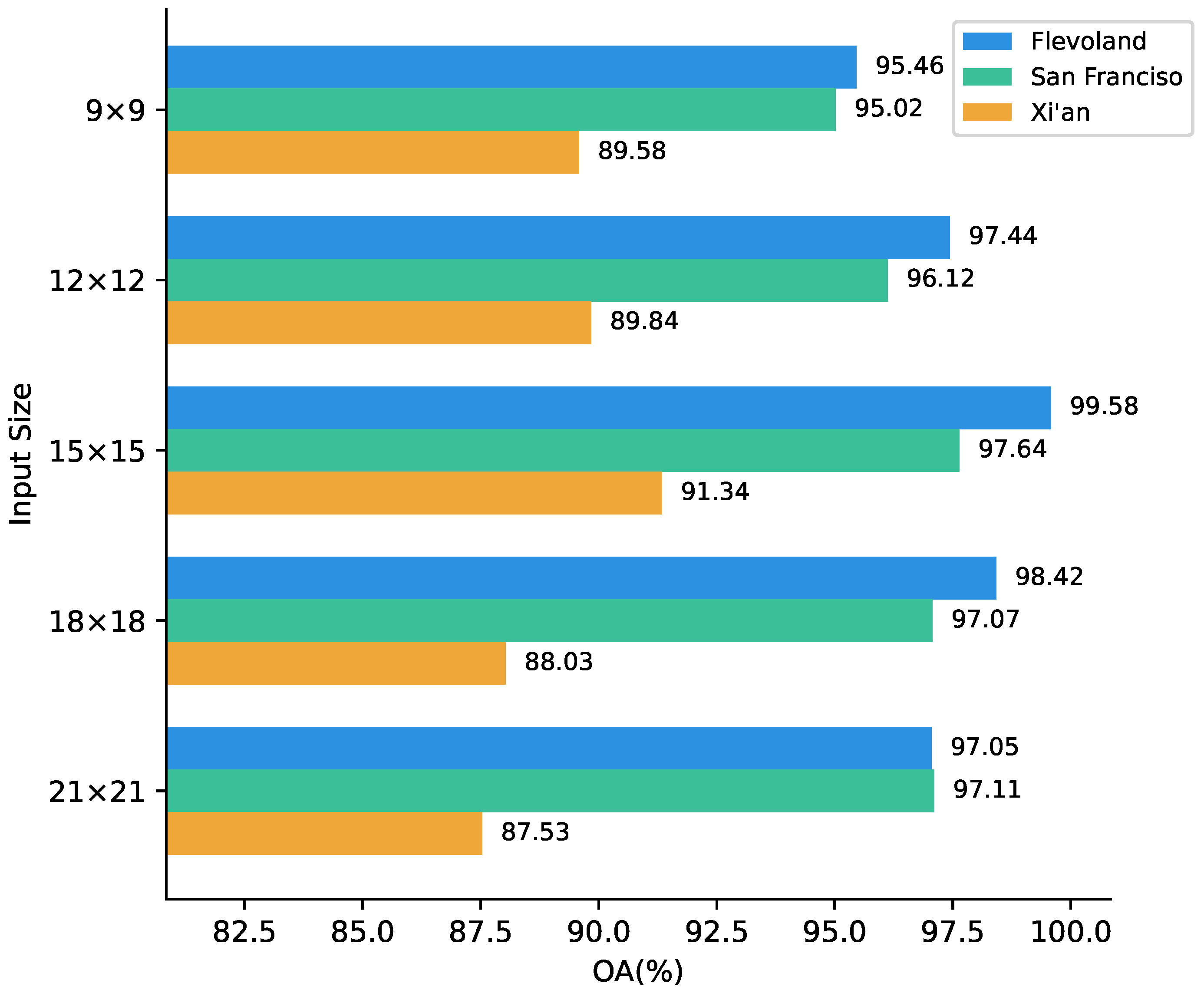
In our experiments, the model was trained on three datasets, Flevoland, San Francisco, and Xi’an, with input image block sizes of 9 × 9, 12 × 12, 15 × 15, 18 × 18, and 21 × 21. The bar chart in Figure 11 shows the results for the different input image block sizes. It can be seen that OA increases as the input image block size grows from 9 × 9 to 15 × 15, and the three datasets reach maximum values when the size is 15 × 15. The Flevoland dataset shows a declining OA trend between block sizes of 15 × 15 and 21 × 21. However, the San Francisco dataset shows a downward trend from a block size of 15 × 15 to one of 18 × 18, but the OA at 21 × 21 increases by 0.419% compared with that at 18 × 18. Similarly, the Xi’an dataset also demonstrates a decrease after peaking at a block size of 15 × 15 as the input block size increases from 15 × 15 to 21 × 21. This decline is attributed to the smaller size of the images within this dataset, which results in incomplete feature extraction as the input size expands.

According to the results on the three datasets, the optimal choice is when the input image block size is 15 × 15.

4.3. Selection of the Amount of Labeled Data for the Three Datasets

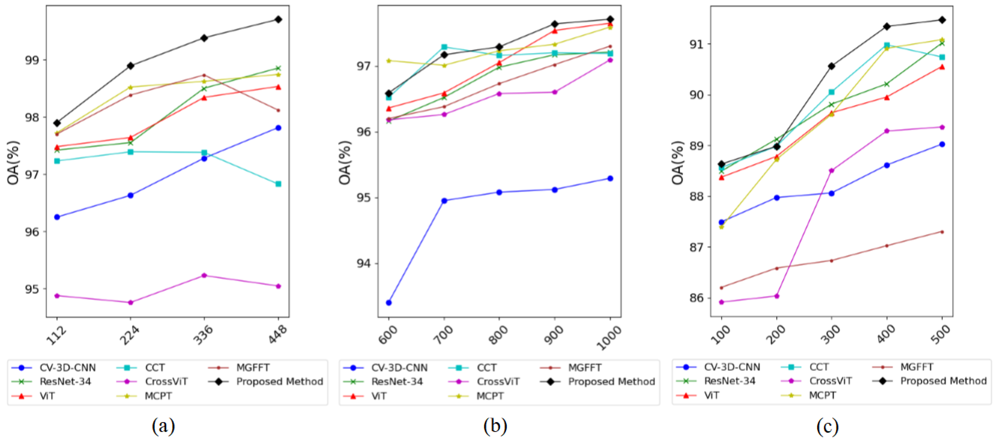
In specific experiments, labeled data from each category within the Flevoland, San Francisco, and Xi’an datasets were randomly sampled at different proportions for training, with details of the sampling shown in Table 6. The classification results for the three datasets are shown in Figure 12. From the line chart, it can be observed that for the Flevoland dataset, as the amount of training data increases from 100 to 300, the OA values of most methods exhibit an upward trend. However, within the range from 300 to 400, the OA values of MGFFT, MCPT, CCT, and CrossViT decline, while those of the remaining methods do not increase significantly. For the San Francisco dataset, the OA values of most methods indicate an increasing trend within the range from 600 to 900, with a larger growth rate than in the range from 900 to 1000. For the Xi’an dataset, the OA values of most methods rapidly increase within the range from 100 to 400, but the growth rate significantly slows down within the range from 400 to 500. Additionally, the OA of CCT decreases within this latter range.

To summarize, for the experiments conducted in this article, the optimal choices for the amount of labeled data for the Flevoland, San Francisco, and Xi’an datasets are 300, 900, and 400, respectively. Furthermore, when using a smaller amount of labeled data, the classification performance of the proposed method is generally superior to that of the other comparison methods.

Figure 11. Relationship between the input size and OA for the proposed method.

Figure 11. Relationship between the input size and OA for the proposed method.

Figure 12. Classification accuracy with different amounts of training data for the three datasets. (a) Flevoland. (b) San Francisco. (c) Xi’an.

Figure 12. Classification accuracy with different amounts of training data for the three datasets. (a) Flevoland. (b) San Francisco. (c) Xi’an.

Table 6. Quantities and corresponding percentages of labeled data.

Flevoland		San Francisco		Xi’an
Quantity	Percentage	Quantity	Percentage	Quantity	Percentage
100	0.89%	600	0.17%	100	0.13%
200	1.17%	700	0.20%	200	0.25%
300	2.68%	800	0.23%	300	0.37%
400	3.57%	900	0.25%	400	0.50%
–	–	1000	0.28%	500	0.63%

Table 6. Quantities and corresponding percentages of labeled data.

Flevoland		San Francisco		Xi’an
Quantity	Percentage	Quantity	Percentage	Quantity	Percentage
100	0.89%	600	0.17%	100	0.13%
200	1.17%	700	0.20%	200	0.25%
300	2.68%	800	0.23%	300	0.37%
400	3.57%	900	0.25%	400	0.50%
–	–	1000	0.28%	500	0.63%

4.4. Impact of Hyperparameters on Model Performance

To investigate the impact of hyperparameters on model performance, this study focuses on the choice of the activation function, optimizer, number of iterations, and learning rate in the context of the AIRSAR Flevoland dataset.

4.4.1. Selection of Activation Function

Activation functions play a crucial role in deep learning models. They not only affect the computational power of the model but also directly influence classification performance.

Table 7. OA results of different activation functions on the Flevoland dataset.

Activation Function	OA
GELU (ours)	0.9958
ReLU	0.9934
Mish	0.9937

shows the OA performance of three activation functions. The activation function used in the proposed model is GELU, which is a smooth activation function that combines the properties of a Gaussian distribution and is widely applicable to transformer networks. We compared GELU with ReLU, a simple nonlinear activation function that is computationally fast and widely used in convolutional neural networks and fully connected networks, and Mish, a newer activation function that is infrequently used compared to the other two but is equally suitable for transformer networks. As shown in Table 7, the OA results of the three activation functions do not differ significantly; ReLU and Mish perform slightly worse than GELU, with both showing a difference of nearly 0.002. The results indicate that the model is not sensitive to the choice of activation function and is robust.

4.4.2. Selection of Optimizer

The OA results of two different optimizers are shown in

Table 8. OA results of different optimizers on the Flevoland dataset.

Optimizer	OA
Adam (ours)	0.9958
SGD	0.9840

. Adam was the optimizer used in our experiments. Adam features a combination of an adaptive learning rate and momentum, making it suitable for most deep learning tasks. With fast and stable convergence, it has been widely utilized as an optimizer in recent years. We compared Adam with SGD, a simple and efficient optimizer that updates parameters using small batches of data but may converge more slowly or exhibit instability. From the OA results in Table 8, it is evident that Adam performs better.

4.4.3. Selection of Number of Iterations

Table 9. OA of different numbers of epochs on the Flevoland dataset.

Epochs	OA
50	0.9857
100 (ours)	0.9958
150	0.9944

demonstrates the effect of three different iteration numbers (50, 100, and 150) on the OA of the model. The relatively low OA results are visible when the number of training epochs is 50, which is due to the incomplete learning of the training set by the model with too few epochs. When the number of training epochs is increased to 150, the OA decreases due to overfitting of the model caused by less training data. Therefore, based on the results in Table 9, 100 training epochs is the appropriate choice.

4.4.4. Selection of Learning Rate

The learning rate plays a critical role in the convergence and performance of deep learning models. Therefore, discussing the learning rate is essential for evaluating the validity of hyperparameter selection. Three commonly used learning rates, $1\times {10}^{-2}$, $1\times {10}^{-3}$, and $1\times 5^{-4}$, were compared with the learning rate of $1\times {10}^{-4}$ adopted in this paper. As shown in Figure 13, the red curve indicates the training loss corresponding to the selected learning rate. It can be seen that the chosen $1\times {10}^{-4}$ learning rate achieves better convergence and a more stable loss trajectory throughout the training process. Specifically, the learning rate chosen in this paper has lower initial loss at the beginning of training compared to the other learning rates and rapidly decreases to converge to zero. The loss curve exhibits smooth behavior during the training process, without noticeable fluctuations.

4.5. Analysis of Computational Cost

In the field of deep learning, differences in computational cost among methods are important for evaluating their practicality and deployability. In order to quantify the computational workload of the eight methods used in the experiments, this study considers the number of floating-point operations (FLOPs), number of parameters (Paras), training time, and prediction time as the core evaluation metrics. Among these, FLOPs directly reflect the computational complexity of the model, while the number of parameters reflects the model’s scale. Training and prediction times reflect the model’s efficiency.

Table 10. Computational cost of the eight methods (using the AIRSAR Flevoland dataset as an example).

Method	FLOPs	Paras	Training Time	Prediction Time
CV-3D-CNN	103.21 M	1.78 M	609.72 s	80.35 s
ResNet-34	62.03 M	850.14 M	529.94 s	52.35 s
SViT	45.88 M	100.62 M	942.70 s	84.51 s
CCT	14.88 M	257.34 M	827.41 s	59.34 s
CrossViT	302.15 M	15.34 M	819.83 s	42.27 s
MCPT	74.91 M	4.10 M	500.32 s	25.81 s
MGFFT	240.71 M	7.02 M	1090.96 s	51.95 s
Proposed	5.82 M	29.06 K	359.82 s	17.44 s

presents the FLOPs, number of parameters, training time, and prediction time calculated for the eight methods evaluated on the AIRSAR Flevoland dataset. It can be clearly seen that the proposed method outperforms the other methods in two key metrics: FLOPs and parameters, demonstrating the lowest computational cost. Additionally, its training and prediction times are relatively short. This low computational cost is mainly due to the method’s deep optimization of the self-attention mechanism and CNN. Through a carefully designed model architecture, this method achieves efficient interaction between internal and external information within a single chunk. This design not only simplifies the model structure but also greatly reduces the complexity of calculating attention relationships between building blocks, thereby significantly lowering overall computational cost. In addition, considering its shorter training and prediction times, the proposed method more comprehensively and efficiently extracts PolSAR data information even with a small amount of labeled data.

5. Conclusions

To address two critical issues in existing deep learning methods for PolSAR image classification, namely the excessive reliance on labeled data and the lack of effective interaction between local and global information, this study proposes a novel method that combines channel-wise convolutional local perception, detachable self-attention, and a residual feedforward network. Specifically, the proposed method comprises several key modules. In the channel-wise convolutional local perception module, channel-wise convolution operations accurately extract local features from different channels of PolSAR images, and local residual connections further enhance these extracted features, providing more discriminative information for subsequent processing. The detachable self-attention mechanism plays a crucial role. It enables effective interaction between local and global information, allowing the model to perceive features at multiple scales and thus improve classification accuracy and robustness. Additionally, replacing the conventional feedforward with a residual feedforward network helps the model better represent local features, enhances gradient propagation across layers, and effectively mitigates the vanishing gradient problem during the training of deep networks. In the final classification stage, the model employs two fully connected layers and incorporates dropout to prevent overfitting, with the softmax function used to generate the final predictions. The effectiveness of the proposed method is evaluated through a combination of objective evaluation metrics and subjective judgment. The results show that, compared with several existing methods, it more effectively extracts local and global features and performs well even with a small amount of labeled data. In addition, it offers significant advantages, including fewer parameters and lower computational complexity, resulting in reduced computational costs to a certain extent and improved classification efficiency. However, the proposed method currently considers only real-valued feature vectors of PolSAR data and does not fully consider factors such as physical scattering characteristics, phase, and amplitude. Therefore, future work could focus on constructing a deep learning model driven by the physical scattering characteristics of PolSAR images and conducting sensitivity analyses of pixel-level processing and feature extraction pipelines, which could have great development potential and research value. Such studies could identify features that most significantly impact model performance, thereby guiding feature selection and ultimately improving classification accuracy in PolSAR image classification.