Class-Discrepancy Dynamic Weighting for Cross-Domain Few-Shot Hyperspectral Image Classification

Abstract

In recent years, cross-domain few-shot learning (CDFSL) has demonstrated remarkable performance in hyperspectral image classification (HSIC), partially alleviating the distribution shift problem. However, most domain adaptation methods rely on similarity metrics to establish cross-domain class matching, making it difficult to simultaneously account for intra-class sample size variations and inherent inter-class differences. To address this problem, existing studies have introduced a class weighting mechanism within the prototype network framework, determining class weights by calculating inter-sample similarity through distance metrics. However, this method suffers from a dual limitation: susceptibility to noise interference and insufficient capacity to capture global class variations, which may lead to distorted weight allocation and consequently result in alignment bias. To solve these issues, we propose a novel class-discrepancy dynamic weighting-based cross-domain FSL (CDDW-CFSL) framework. It integrates three key components: (1) the class-weighted domain adaptation (CWDA) method dynamically measures cross-domain distribution shifts using global class mean discrepancies. It employs discrepancy-sensitive weighting to strengthen the alignment of critical categories, enabling accurate domain adaptation while maintaining feature topology; (2) the class mean refinement (CMR) method incorporates class covariance distance to compute distribution discrepancies between support set samples and class prototypes, enabling the precise capture of cross-domain feature internal structures; (3) a novel multi-dimensional feature extractor that captures both local spatial details and continuous spectral characteristics simultaneously, facilitating deep cross-dimensional feature fusion. The results in three publicly available HSIC datasets show the effectiveness of the CDDW-CFSL.

1. Introduction

Hyperspectral images (HSIs) consist of continuous spectral bands and provide rich, detailed spectral–spatial information [1,2,3]. This unique characteristic has facilitated their extensive application in precision agriculture [4], land-use classification [5], and urban planning [6]. As a key technology in these applications, hyperspectral images classification (HSIC), which assigns pixels to different categories, plays a crucial role and has attracted significant research attention in recent years [7,8]. Many deep learning models have emerged especially for this purpose as a result of the notable advancements made in HSI-based land-cover categorization due to the quick growth of deep learning. Convolutional neural networks (CNNs), a well-known deep learning technique, have excelled in hyperspectral image categorization among them [9,10,11,12,13,14,15].

Notably, while the aforementioned deep learning approaches have demonstrated progress in HSIC, they generally require substantial quantities of labeled samples. To address the label insufficiency problem in hyperspectral data, researchers have adopted both semi-supervised [16,17,18,19] and unsupervised learning [20,21,22,23] strategies. Zheng et al. [24] employed semi-supervised learning for pseudo-label generation, achieving significant improvements in minority class classification accuracy, particularly in severely imbalanced datasets. Wang et al. [25] proposed an enhanced semi-supervised classification framework that tackles label scarcity by integrating active deep learning with random multi-graph algorithms. Zhang et al. [26] introduced an unsupervised multi-scale diverse feature learning (UMsDFL) method that synergistically combines CNN architectures with superpixel segmentation, effectively fusing multi-scale features with spectral information to substantially boost classification accuracy, thereby providing innovative solutions for HSIC.

While these methods effectively reduce reliance on annotated data, they often struggle to achieve accurate class discrimination when encountering novel categories absent from the training phase due to limited prior knowledge. In recent years, the effective learning process of the human visual system has sparked interest in few-shot learning (FSL) for HSIC. The ability of FSL to recognize new classes with extremely limited labeled samples makes it particularly attractive [27,28,29,30]. As a fundamental FSL paradigm, meta-learning enables rapid adaptation to new tasks by simulating multi-task learning processes. This approach has driven extensive applications of metric-based and embedding-based methods in HSIC [31,32,33,34]. Liu et al. [35] proposed a deep few-shot learning (DFSL) framework that leverages Euclidean distance metrics and nearest-neighbor classification to effectively tackle sample scarcity in hyperspectral imagery. Xi et al. [36] developed a FSL approach named CMFSL, which enhances classification performance under limited annotations via Mahalanobis distance optimization and class covariance estimation. Tang et al. [37] introduced a deep fuzzy metric learning method that employs fuzzy logic with Gaussian membership functions to establish robust distance metrics for addressing class uncertainty in HSIC.

Even though the current FSL methods demonstrate improved classification accuracy for novel categories with limited labeled samples, they predominantly rely on the strong assumption of identical data distributions between source domains $\left(\mathrm{SD}\right)$ and target domains $\left(\mathrm{TD}\right)$ [38,39,40,41]. However, practical applications frequently encounter domain shift issues caused by sensor variations and environmental changes [42,43], which substantially compromise model generalization capabilities. To address this challenge, Li et al. [44] pioneered a deep cross-domain FSL (DCFSL) framework that effectively mitigates distribution discrepancies in HSIC through domain adaptation strategies. Their approach outperforms conventional methods when TD samples are scarce. Additionally, Hu et al. [45] proposed a dual modulation cross-modality (DMCM) meta-learning approach, which integrates a 3D ghost attention network with class covariance metric, achieves significant accuracy improvements in cross-domain FSL scenarios. Similarly, Zhang et al. [46] developed a few-shot graph aggregation framework that aligns cross-domain non-local relationships through dynamic feature extraction. Finally, Qin et al. [47] proposed a feature disentanglement-based FSL (FDFSL) method that utilizes multi-order interaction and self-distillation strategies to reduce SD bias while enhancing TD feature learning in HSIC.

Although the aforementioned domain adaptation methods have partially addressed the domain shift problem, several limitations remain. Primarily, these approaches usually prioritize matching global feature distributions across SD and TD, ignoring the significance of accomplishing local feature alignment across various class-wise data distributions [48,49,50]. To overcome these limitations, Ye et al. [51] proposed an adaptive adversarial FSL (ADAFSL) framework that employs adaptive weight allocation and multi-scale feature extraction, prioritizing domain adaptation for classes exhibiting higher distribution mismatches between SD and TD. Similarly, Feng et al. [52] proposed a CCGDA approach, which simultaneously addresses both class imbalance and domain shift challenges through the coordinated optimization of a hierarchical capsule network and an adaptive sampler. Finally, the proposed global–local graph attention network (GLGAT-CFSL) [53] tackles domain adaptation in HSIC by utilizing dynamic triplet graph attention networks and local similarity learning, offering novel insights for future research directions.

Though current cross-domain few-shot learning methods based on domain adaptation have achieved certain success in feature matching through local feature alignment strategies, further mitigating the domain shift problem, their core alignment strategies still exhibit significant limitations. Specifically, when partial class overlap occurs between source and target domains, the sample distribution becomes imbalanced, some categories in the target domain suffer from extreme data scarcity, while others remain relatively sufficient. To address this issue, existing studies have proposed class-weighting methods. However, these methods relying solely on distance metrics for weight calculation fail to comprehensively characterize global cross-domain class differences, resulting in distorted weight allocation for certain categories. Furthermore, conventional hyperspectral feature extraction methods are generally incapable of simultaneously capturing continuous spectral information and local spatial features, leading to the loss of critical detailed information.

To overcome the drawbacks of the previously described domain adaptation methods, we propose a novel cross-domain FSL framework based on class-discrepancy dynamic weighting (CDDW-CFSL) for domain-adaptive HSIC tasks. Firstly, the proposed class-weighted domain adaptation (CWDA) method dynamically assigns class-specific weights through calculating the mean discrepancy of corresponding categories between SD and TD. This approach enables a preferential focus on categories with more significant discrepancies between the source domain and the target domain during the domain adaptation phase. Furthermore, to ensure samples of the same class are more compact and make the class weights calculated by class means during the domain adaptation stage more representative, a class mean refinement (CMR) method is proposed. This approach imposes constraints on class prototypes, thereby providing more reliable class prototypes for subsequent domain adaptation. In addition, the framework introduces a cross-dimensional feature extraction mechanism, which mainly consists of the efficient multi-scale dimensional feature fusion (EMDF) method. The method separates hyperspectral imagery channel-wise into distinct components and then utilizes differently sized convolution kernels to derive features from every partitioned section. This allows for the effective integration of spectral and spatial information; more generalized and semantically rich feature representations are constructed across the source and target domains. By combining these multi-dimensional features, the framework facilitates feature alignment between SD and the TD. Finally, the framework can transfer knowledge across the rich labeled information in the SD and the limited labeled information in TD, thanks to the framework’s integration of the previously described methods and simultaneous FSL operations on SD and TD.

This work offers the following significant contributions:

• The proposed CWDA method calculates global class mean discrepancy to assign weights by directly comparing class centroid distances between SD and TD, effectively overcoming the limitations of conventional distance metric methods. This approach enables domain adaptation to more accurately identify and focus on categories with significant distribution discrepancies between SD and TD.
• To enhance the accuracy of class mean calculations, the CMR method innovatively computes the covariance distance between support set samples and class prototypes by incorporating class covariance distance. This enables a deeper analysis of the internal distribution characteristics within each class, allowing the final calculated class means to more accurately reflect the overall distribution properties of the categories.
• We propose a novel EMDF method that simultaneously captures local spatial details and continuous spectral information via a collaborative parallel multi-path structure. In addition to improving the extraction of complementary features, this structure successfully maintains the original data. Moreover, the method enables multi-perspective spectral and spatial feature extraction and integrates spectral–spatial information through multi-level feature fusion.

This study first systematically elaborates on the proposed CDDW-CFSL framework in Section 2, followed by the validation of the method’s effectiveness through extensive experiments in Section 3. Section 4 explores the features and benefits of the suggested approach. Section 5 concludes by summarizing the entire work and offering a prediction for future lines of inquiry.

2. Methods

In this section, we provide a comprehensive overview of the suggested method. As illustrated in Figure 1, the entire framework consists of a mapping layer, an integrated cross-dimensional feature extractor, an FSL module, a class-weighted domain adaptation (CWDA) method, and a class mean refinement (CMR) method. Firstly, the SD and TD are separated into support and query sets, respectively, and the mapping layer aligns SD and TD features into a shared feature space. Furthermore, the cross-dimensional feature extraction that was created is then used to thoroughly mine both spatial and spectral data, facilitating cross-modal interaction between spatial and spectral information. Additionally, FSL operations are performed on the data from SD and TD based on Euclidean distance, effectively achieving cross-domain knowledge transfer. Finally, to avoid the excessive reliance on local sample pairs in traditional methods, we propose a CWDA method. This method dynamically quantifies cross-domain local distribution shifts based on global class mean discrepancy, enabling a more comprehensive capturing of distribution discrepancies across domains and more effective local feature alignment between SD and TD. In addition, to ensure that the calculated sample means can more accurately reflect the true feature distribution of each class, we introduce the CMR method. This method optimizes the allocation of class prototypes in the feature space, reducing the biases introduced via cross-domain shifts.

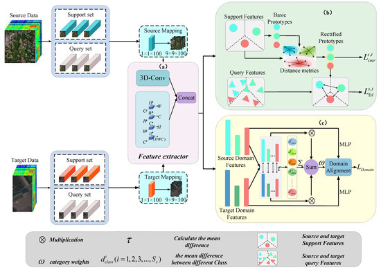
Figure 1. Overall framework of the proposed CDDW-CFSL in the training phase. Including data preprocessing; (a) EMDF and FSL; (b) CMR; (c) CWDA.

During the testing phase, as illustrated in Figure 2, we classify the unlabeled samples in TD. Initially, the dimensionality of the input samples is adjusted to match that of the training phase via a mapping layer. Subsequently, the cross-dimensional feature extractor is employed to extract features from the input samples. Ultimately, these unlabeled data are classified using the K-nearest neighbor (K-NN) classifier.

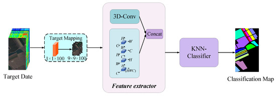
Figure 2. Overall framework of the proposed CDDW-CFSL in the testing phase.

2.1. Data Preprocessing

We typically represent HSI from SD and TD as ${R_1}^{H_1\times W_1\times c{h}_1}$ and ${R_2}^{H_2\times W_2\times c{h}_2}$, where $R_1$ and $R_2$ represent the datasets of SD and TD, respectively, $H_1$, $H_2$, $W_1$, and $W_2$ denote the height and width of SD and TD images, respectively, $c{h}_1$ and $c{h}_2$ reflect SD and TD spectral dimensions. Firstly, take SD as an example; we extract a 3D pixel block centered on each pixel with a size of $r_1^{9\times 9\times c{h}_1}$ from ${R_1}^{H_1\times W_1\times c{h}_1}$; similarly, we perform the same operation on TD to extract a 3D pixel block of size $r_2^{9\times 9\times c{h}_2}$. Furthermore, to simulate the real FSL scenario, we divide the data of SD and TD into support sets and query sets. The method is trained on the support set, and its performance is assessed on the query set. Finally, to address the issue of spectral resolution mismatch between SD and TD caused by different imaging conditions or sensor differences. Prior to feature extraction, a mapping layer is adopted in our framework, which maps both SD and TD spectral features into an identical 100-dimensional representation space for dimensionality unification. Following processing through this mapping layer, the input data from the source domain (SD) is transformed into a tensor of $r_1^{9\times 9\times 100}$, while the input data from the target domain (TD) is converted into a tensor of $r_2^{9\times 9\times 100}$, where $9\times 9$ represents spatial dimensions and 100 denotes spectral dimensionality. This dimensional alignment strategy effectively mitigates spectral resolution discrepancies caused by sensor variations, ensuring data comparability between domains within a unified feature space. The standardized representation establishes a fundamental basis for subsequent cross-domain feature alignment and knowledge transfer.

2.2. Cross-Dimensional Feature Extraction

In cross-domain HSIC tasks, due to factors such as sensor differences, the SD and TD may exhibit not only spectral resolution discrepancies but also distinct feature distributions and data representations. Therefore, we propose a cross-dimensional feature extraction, our method simultaneously captures local spatial details and continuous spectral information, enabling the better identification of shared features across domains. The model demonstrates markedly improved operational efficacy and enhanced cross-domain generalization when applied to TD. The proposed feature extractor is illustrated in Figure 3. The feature extractor takes the output of the mapping layer as input, comprising two residual blocks, two max-pooling layers, and a convolutional layer. The residual blocks integrate 3D-CNN and the efficient multi-scale dimensional feature fusion (EMDF) method to thoroughly leverage the spatial–spectral characteristics of HSI. During feature extraction, the 3D-CNN extracts shallow features to capture the overall spatial structure of the image, which can be concisely represented as follows:

$$r^{\prime }=ReLu(BatchNorm3d\left(Conv3d\left(r\right)\right)$$

(1)

where r is the output of the mapping layer, $r^{\prime }$ is the output of $Conv3D\left(r\right)$, $Conv3D\left(r\right)$ is the convolution operation, and $ReLu\left(\right)$ is the activation function.

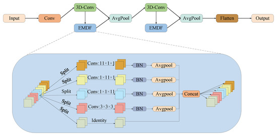
Figure 3. Proposed EMDF method.

Additionally, to capture multi-scale features and reveal relationships between different dimensions, we use the EMDF method to deeply explore deeper-level information in the output features of the mapping layer across different dimensions. Then, we concatenate the features extracted via the 3D-CNN and EMDF method, allowing the model to understand and analyze hyperspectral images from different perspectives and improving the classification accuracy. The input to the EMDF method is the output from the 3D-CNN. Given an input tensor of dimensions C × H × W, firstly, we divide the input into five parts along the channel dimension. Furthermore, the first part remains unchanged; the second part captures interaction information between channel dimensions C, H, and W, while the third, fourth, and fifth parts use depthwise convolution operations with kernel sizes of $11\times 1\times 1$, $1\times 11\times 1$, and $1\times 1\times 11$, respectively, to process the channel, width, and height dimensions. Finally, we concatenate the results of the five parts along the channel dimension, which can be simply represented as follows:

$$\begin{array}{cc}\hfill (r_{id},r_{\mathrm{chw}},r_c,r_h,r_w)& =\mathrm{split}(r^{\prime },(g{c}_1,g{c}_2,\dots ,g{c}_5),\dim =1)\hfill \end{array}$$

(2)

$$x_{chw},x_c,x_h,x_w=Conv3D(r_{\mathrm{chw}},r_c,r_h,r_w)$$

(3)

where $g{c}_i=20(i=1,2,\dots ,5)$ represents the spectral dimension of each partitioned component after $r^{\prime }$ is divided equally along the channel dimension, $\mathrm{split}(·)$ represents the spectral segmentation function, and $x_{chw},x_c,x_h,x_w$ represents the output features obtained by each part through $Conv3D$. Finally, the results of the five parts are concatenated along the channel dimension, and we concatenate the outputs from both the 3D-CNN and EMDF method, which can be simply represented as follows:

$$x^{\prime }=cat(r_{id},x_{chw},x_c,x_h,x_w)$$

(4)

$$x=cat(r^{\prime },x^{\prime })$$

(5)

where $cat$ represents the channel-wise concatenation operation, $x^{\prime }$ represents the output result of the EMDF method, and X represents the output result of the residual connection between the 3D-CNN and EMDF method.

The EMDF method utilizes multi-branch depthwise separable convolutions to extract features from different dimensions, aiming to capture more complex spatial and spectral features in HSI. This enables a more effective extraction of cross-domain shared features and enhances the model’s generalization performance in the TD.

2.3. FSL in Source and Target Domains

In cross-domain HSIC tasks, there are usually very few labeled samples in TD. The model can more effectively mine transferable information from SD when FSL is performed in both SD and TD. This increases the model’s capacity to handle unknown classes in TD in addition to its ability to generalize to new classes. Consequently, subsequent to feature extraction, we instantiate meta-learning-based FSL in both SD and TD. We assume that the source domain dataset is (SD) (containing classes $C_s$) and that the target domain dataset (TD) is (containing classes $C_t$). Specifically, taking FSL in SD as an example, we randomly select classes $S_s$ from $C_s$ SD’s classes, with each class containing k labeled samples as the support set $Z_s={(x_i,y_i)}_{i=1}^{S_{s\times k}}$. Then, we randomly select t unlabeled samples from the same $S_s$ classes as the query set $Q_s={(x_j,y_j)}_{j=1}^{S_{s\times t}}$. In each FSL task, we apply FSL by figuring out the Euclidean distance between each class prototype and the query set samples, and then we use the $Softmax$ function to find the estimated likelihood of the query set samples; this may be represented as follows:

$$P(y_j=k|x_j\in Q_s)=Softmax(-d(f\phi \left(x_j\right),P_k))$$

(6)

where $P_k$ is the revised prototype of the $k\text{-}\mathrm{th}$ class, $x_i$ and $y_i$ represents the sample set in the support set, and $x_j$ and $y_j$ represent the sample set in the query set, $P(y_j=k|x_j\in Q_s)$ represents the predicted probability of the query set samples, $d\left(\right)$ represents the Euclidean distance, and $f\phi \left(x_j\right)$ represents the probability that the model predicts the query set sample $x_j$ as a certain class.

Based on the predicted probabilities of the query set samples, the loss function of FSL in SD can be expressed as follows:

$$L_{fsl}^s={\displaystyle \frac{{\sum }_{(x,y)\in Q_s}logP(y_j=k|x_j\in Q_s)}{\mid Q_s\mid }}$$

(7)

where $Q_s$ symbolizes the magnitude of the query set in SD, and $L_{fsl}^s$ is the FSL loss value in SD.

Similarly, the expression for the FSL loss function in TD is as follows:

$$L_{fsl}^t={\displaystyle \frac{{\sum }_{(x,y)\in Q_t}logP(y_j=k|x_j\in Q_t)}{\mid Q_t\mid }}$$

(8)

where $Q_t$ symbolizes the magnitude of the query set in TD, and $L_{fsl}^t$ is the FSL loss value in TD.

In summary, the following is the overall loss of FSL in SD and TD:

$$L_{\mathrm{fsl}}=L_{\mathrm{fsl}}^s+L_{\mathrm{fsl}}^t$$

(9)

2.4. Class-Weighted Domain Adaptation

Current FSL can transfer known knowledge from SD to TD by performing FSL simultaneously in both SD and TD when labeled samples in TD are limited, thereby improving the model’s performance in TD. However, in real-world cross-domain HSIC tasks, factors such as variations in lighting and sensor differences lead to inconsistent distributions between SD and TD. Moreover, the degree of distribution shift and the number of samples vary significantly across different categories. As shown in Figure 4a, the existing methods typically rely on distance metrics to calculate class weights for achieving local feature alignment. For categories with relatively stable spectral–spatial features (e.g., categories $C_3$ and $C_4$), basic alignment can be achieved. However, for categories with complex nonlinear structures (e.g., categories $C_1$ and $C_2$), traditional methods often struggle to achieve ideal matching results during local feature alignment.

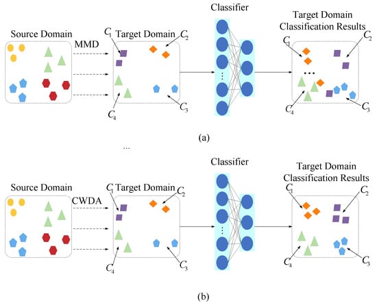
Figure 4. Class-level domain adaptation. (a) Using regular MMD; (b) using class-weighted MMD.

Therefore, this paper proposes a class-weighted domain adaptation (CWDA) method. Unlike conventional approaches, as illustrated in Figure 4b, our proposed CWDA method employs global inter-class mean discrepancy to dynamically quantify cross-domain local distribution shifts. This enables the model to more precisely focus on categories exhibiting significant distribution differences between SD and TD. The method takes features extracted via the feature extractor from both domains as input. Specifically, it first performs domain adaptation between SD and TD using Maximum Mean Discrepancy (MMD). Subsequently, it calculates the feature means for each class in both the source and target domains separately. An element-wise subtraction operation is then applied to obtain a cross-domain class mean discrepancy matrix, which serves as a quantitative representation of distribution shifts. The empirical formulation of MMD is expressed as follows:

$$\begin{array}{cc}\hfill L_{mmd}(X,Y)& ={\displaystyle \frac{1}{n^2}}\sum _{i=1}^n\sum _{j=1}^{n}k(x_{si},x_{sj})+\hfill \\ \hfill & {\displaystyle \frac{1}{m^2}}\sum _{i=1}^m\sum _{j=1}^{m}k(x_{ti},x_{tj})-{\displaystyle \frac{2}{nm}}\sum _{i=1}^n\sum _{j=1}^{m}k(x_{si},x_{tj})\hfill \end{array}$$

(10)

where $(X,Y)$ are the sample sets of SD and TD, respectively, $x_s=\{x_{s1},\dots ,x_{si},\dots ,x_{sn}\}$ represents the SD sample, $x_t=\{x_{t1},\dots ,x_{tj},\dots ,x_{tm}\}$ represents the TD sample, n represents the number of samples in the SD, m represents the number of samples in the TD, $k(x_{si},x_{sj})$ represents a kernel function that measures the similarity within SD samples, while $k(x_{si},x_{tj})$ measures the similarity between SD and TD samples. The SD and TD class means are shown as follows:

$$m_{sou}={\displaystyle \frac{1}{N_{sou}}}\sum _{i=1}^{N_{sou}}{x}_{sou}^i$$

(11)

$$m_{tar}={\displaystyle \frac{1}{N_{tar}}}\sum _{i=1}^{N_{tar}}{x}_{tar}^j$$

(12)

where $N_{sou}$ and $N_{tar}$, respectively, represent the number of samples in the corresponding classes of the SD and the TD, respectively, $x_{sou}^i$ and $x_{tar}^j$, respectively, represent the i-th sample belonging to the corresponding class in the SD and the j-th sample belonging to the corresponding class in the TD.

$$d_{class}=\mid m_{sou}-m_{tar}\mid$$

(13)

where $d_{class}$ represents the class difference between SD and TD.

Additionally, we compute class weights using a cross-domain feature weighting strategy. Specifically, first, we divide the mean difference of each corresponding class between the source and target domains by the sum of the mean differences across all classes. Furthermore, we divide the mean of each class in SD by the sum of the mean differences of all classes in SD. Finally, we perform a weighted summation of the results from the above two steps to obtain the corresponding class weights. Based on this process, the weight calculation formula can be expressed as follows:

$$w_{class}=(1-\alpha ){\displaystyle \frac{d_{class}}{{\sum }_{i=1}^{S_s}{d}_{class}^i}}+\alpha {\displaystyle \frac{m_{sou}}{{\sum }_{i=1}^{S_s}{m}_{sou}^i}}$$

(14)

Finally, by performing element-wise multiplication between the maximum mean discrepancy (MMD) loss and class weights, we exert different influences on the MMD loss in the class dimension, enabling classes with greater alignment difficulty to obtain stronger optimization intensity. This achieves true class-level weighting. It can effectively guide the model to pay more attention to classes with significant distribution shifts, thereby improving the overall cross-domain alignment effect. This can be simply expressed as follows:

$$L_{\mathrm{domain}}=(1-\alpha )L_{\mathrm{mmd}}+\alpha L_{\mathrm{mmd}}\times w_{\mathrm{class}}$$

(15)

where $L_{\mathrm{mmd}}$ is the $L_{\mathrm{MMD}}$-calculated difference between SD and TD, $w_{\mathrm{class}}$ is the class weight, and $\alpha$ is the weight coefficient.

2.5. Class Mean Refinement

The proposed class-weighted domain adaptation (CWDA) method computes class means to transfer information from SD and TD. However, in few-shot learning, due to limited TD samples and noise, the alignment of local features exhibits suboptimal matching, causing suboptimal alignment. Therefore, this paper proposes a class mean refinement (CMR) method, as illustrated in Figure 1b, which leverages inter-class covariance distance to refine class prototypes. By capturing the intrinsic distribution characteristics within categories, this approach enhances the representativeness of prototypes. This mechanism strengthens the class weighting effect, enables more precise feature alignment, and consequently improves the generalization performance in cross-domain few-shot learning. The CMR method can be formally expressed as follows:

$$D_{\mathrm{md}}(x_i,c_k)={(x_i-c_k)}^T{\sum }_C^{-1}(x_i-c_k)$$

(16)

$$P_k=Softmax\left(D_{\mathrm{md}}(x_i,c_k)\right)$$

(17)

where $D_{\mathrm{md}}$ is the class covariance distance, $c_k$ represents the basic class prototype, and $P_k$ represents the probability forecast of the support set samples, which is the rectified class prototype. Based on the prediction results of the support set samples, the loss in SD is as follows:

$$L_{cmr}^s={\displaystyle \frac{-{\sum }_{(x,y)\in Z_s}log{P}_k}{|Z_s|}}$$

(18)

Similarly, the loss in the target domain is as follows:

$$L_{cmr}^t={\displaystyle \frac{-{\sum }_{(x,y)\in Z_t}log{P}_k}{|Z_t|}}$$

(19)

In summary, the following is the overall loss of cmr in SD and TD:

$$L_{\mathrm{cmr}}=L_{\mathrm{cmr}}^s+L_{\mathrm{cmr}}^t$$

(20)

Consequently, the complete loss function of SD may be formulated as follows:

$$L_{\mathrm{s}}=L_{\mathrm{fsl}}^s+L_{\mathrm{cmr}}^s+L_{\mathrm{domain}}$$

(21)

Similarly, the complete loss function of TD may be formulated as follows:

$$L_{\mathrm{t}}=L_{\mathrm{fsl}}^t+L_{\mathrm{cmr}}^t+L_{\mathrm{domain}}$$

(22)

3. Experiments

We performed comprehensive cross-domain hyperspectral classification experiments across four benchmark datasets to rigorously evaluate the efficacy of our proposed CDDW-CFSL framework. This section details the datasets and experimental configurations, and it analyzes the experimental results.

3.1. Dataset Description

3.1.1. Source Domain Dataset

The Chikusei dataset was captured via an airborne imaging spectrometer (Headwall Hyperspec VNIR) in Chikusei City, Japan. With a picture size of 2517 by 2335 pixels and an exterior sampling distance of 2.5 m, the image has 128 bands of spectrum that span the wavelength range of 363 nm to 1080 nm. Nineteen land cover types, such as rice fields, woods, highways, etc., are included in the dataset. Each land cover class’s names and sample numbers are included in Table 1, and the pseudo-color composite picture and matching ground truth map are displayed in Figure 5.

Table 1. Land cover classes and sample counts in the Chikusei dataset.

Class	Name	Samples
1	Water	2845
2	Bare soil (school)	2859
3	Bare soil (park)	286
4	Bare soil (farmland)	48,525
5	Natural plants	4297
6	Weeds in farmland	1108
7	Forest	20516
8	Grass	6515
9	Rice field (grown)	13,369
10	Rice field (first stage)	1268
11	Row crops	5961
12	Plastic house	2193
13	Manmade (non-dark)	1220
14	Manmade (dark)	7664
15	Manmade (blue)	431
16	Manmade (red)	222
17	Manmade grass	1040
18	Asphalt	801
19	Paved ground	145
Total		77,592

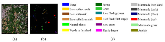
Figure 5. Chikusei dataset. (a) Ground-truth image. (b) Pseudo-color composite image. (c) Corresponding color labels.

3.1.2. Target Domain Datasets

NASA’s AVIRIS (Airborne Visible/Infrared Imaging Spectrometer) sensor collected the Indian Pines (IP) dataset in a northwest Indiana agricultural region. Farmland makes up the majority of the region, with a small amount of woodland and urban structures. The scene size is $145\times 145$ pixels, and the spatial resolution is 20 m (each pixel represents a ground area of $20\times 20$ m). There are 202 spectral bands in the picture, spanning the 400–2500 nm range. There are sixteen land cover categories in the dataset, such as woods, railroads, and residential areas. Each land cover class’s names and sample numbers are included in Table 2, and the pseudo-color composite picture and matching ground truth map are displayed in Figure 6.

Table 2. Land cover classes and sample counts in the Indian Pines Dataset.

Class	Name	Samples
1	Alfalfa	46
2	Corn-notil	1428
3	Corn-mintill	830
4	Corn	237
5	Grass-pasture	483
6	Grass-trees	730
7	Grass-pasture-mowed	28
8	Hay-windrowed	478
9	Oats	20
10	Soybean-notill	972
11	Soybean-mintill	2455
12	Soybean-clean	593
13	Wheat	205
14	Woods	1265
15	Buildings-Grass-Trees-Drives	386
16	Stone-Steel-Towers	93
Total		10,249

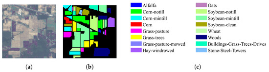
Figure 6. Indian Pines dataset. (a) Ground-truth image. (b) Pseudo-color composite image. (c) Corresponding color labels.

The Pavia University (PU) dataset was captured via the ROSIS (Reflective Optics System Imaging Spectrometer) sensor near the University of Pavia, Italy. The region is mostly made up of agricultural and urban areas. With a scene size of $610\times 340$ pixels and a spatial resolution of 1.05 m, the image includes 103 spectral bands that span the wavelength range of 430–860 nm. Nine land cover types, such as highways, woods, and mining regions, are included in the dataset. Each land cover class’s names and sample numbers are included in Table 3, and the pseudo-color composite picture and matching ground truth map are displayed in Figure 7.

Table 3. Land cover classes and sample counts in the Pavia University Dataset.

Class	Name	Samples
1	Asphalt	6631
2	Meadows	18,649
3	Gravel	2099
4	Trees	3064
5	Painted metal	1345
6	Bare Soil	5029
7	Bitumen	1330
8	Self-blocking	3682
9	Shadows	947
Total		42,776

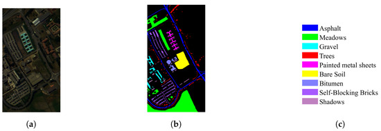
Figure 7. Pavia University dataset. (a) Ground-truth image. (b) Pseudo-color composite image. (c) Corresponding color labels.

The Salinas dataset (SA) was captured via the AVIRIS sensor in an agricultural area in California, USA. With a scene size of $512\times 217$ pixels and a resolution in space of $3.7$ m, the image has 224 spectral bands that span the 400 nm to 2500 nm range. Sixteen land cover categories, such as farms, irrigated regions, grasslands, etc., are included in the dataset. Each land cover class’s names and sample numbers are included in Table 4, and the pseudo-color compound picture and matching ground truth map are displayed in Figure 8.

Table 4. Land cover classes and sample counts in the Salinas Dataset.

Class	Name	Samples
1	Brocoli-green-weeds-1	2009
2	Brocoli-green-weeds-2	3726
3	Fallow	1976
4	Fallow-rough-plow	1394
5	Fallow-smooth	2678
6	Stubble	3959
7	Celery	3579
8	Grapes-untrained	11,271
9	Soil-vinyard-develop	6203
10	Corn-senesced-green-weeds	3278
11	Lettuce-romaine-4wk	1068
12	Lettuce-romaine-5wk	1927
13	Lettuce-romaine-6wk	916
14	Lettuce-romaine-7wk	1070
15	Vinyard-untrained	7268
16	Vinyard-untrained-trellis	1807
Total		54,129

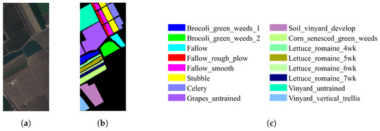
Figure 8. Salinas dataset. (a) Ground-truth image. (b) Pseudo-color composite image. (c) Corresponding color labels.

3.2. Experimental Setup

All experiments were conducted on a computing platform equipped with an NVIDIA GeForce RTX 3060 GPU (NVIDIA Corporation, Santa Clara, CA, USA), 64 GB of RAM, and an Intel Core i7-10700 processor with a base clock speed of 2.90 GHz (Intel Corporation, Santa Clara, CA, USA). The software environment employed the PyTorch framework, with Python 3.9 and PyTorch 2.3.0 used. Following the experimental configuration described in [52], we randomly selected 200 labeled samples per class from the source domain dataset to construct the source dataset for transferable knowledge learning, while L = 5 labeled samples per class were randomly chosen from the target dataset for training. Input data was processed in the form of 9 × 9 × 100 image patches. For feature extraction across both SD and TD, the network’s convolutional layers were trained using the Adam optimizer. The model underwent 10000 training iterations to ensure thorough convergence, with a steady learning rate of 0.001 to maintain training stability and mitigate overfitting.

During the FSL phase, the HSIC task is decomposed into multiple C-way K-shot classification sub-tasks (where C denotes the number of classes in each episode’s support set, and K indicates the number of samples per class). The support set comprises 1 sample per class, whereas the query set contains 19 samples per class. Theoretically, increasing the number of query samples improves the network’s classification performance on TD. Three metrics are adopted for evaluation: the Kappa coefficient (Kappa), average accuracy (AA), and the overall accuracy (OA).

3.3. Ablation Study

In this part, we examine how the performance of the TD dataset is affected by significant components of the suggested framework. This innovative framework primarily consists of three core methods: (1) the basic few-shot learning (FSL) module, responsible for extracting cross-domain shared feature representations; (2) the class-weighted domain adaptation (CWDA) method, which achieves adaptive domain alignment based on class importance; and (3) the class mean refinement (CMR) method, designed to refine class prototype representations. To thoroughly examine the individual contributions and synergistic effects of each module, first constructing a baseline module containing only the FSL module (FSL-only) and then sequentially integrating the CWDA method to form an intermediate FSL + CWDA module, we add the CMR method to create a comparative FSL + CMR module and finally combine them into the complete framework (FSL + CWDA + CMR).

The findings of the ablation investigation are shown in Table 5, Table 6 and Table 7. Using the PU dataset as an example, the introduction of the CWDA method, which incorporates an adaptive class-weighting mechanism, leads to a notable improvement of 2%–3% in overall accuracy (OA), demonstrating the critical role of cross-domain class-weight adjustment in performance enhancement. Further integrating the CMR method, which optimizes the feature space distribution of classes, elevates the OA to 87.99%, validating the effectiveness of fine-grained feature alignment. Most importantly, the complete framework achieves a consistent 4% performance gain over the baseline model. This outcome not only validates the effectiveness of each method’s design but also reveals a synergistic enhancement effect among them. The organic integration of FSL’s feature extraction, CWDA’s domain adaptation, and CMR’s representation optimization can significantly mitigate domain shift in deep domain adaptation. These results fully demonstrate that the collaborative operation of these methods effectively alleviates the negative impact caused by domain shift.

Table 5. Ablation experiments through combinations of modules on the Indian Pines Dataset.

Metric	Only FSL	FSL + CWDA	FSL + CMR	Our
OA	74.34 ± 0.45	76.89 ± 0.48	77.96 ± 0.23	81.23 ± 0.97
AA	78.58 ± 0.52	85.50 ± 0.45	85.67 ± 0.05	86.01 ± 0.48
Kappa	65.86 ± 0.42	73.81 ± 0.55	74.94 ± 0.25	75.50 ± 0.61

Table 6. Ablation experiments through combinations of modules on the Pavia University Dataset.

Metric	Only FSL	FSL + CWDA	FSL + CMR	Our
OA	85.72 ± 0.96	87.16 ± 1.23	87.99 ± 0.73	89.68 ± 0.54
AA	83.57 ± 0.68	85.27 ± 0.68	85.70 ± 0.65	86.17 ± 0.41
Kappa	80.78 ± 1.29	82.73 ± 1.66	83.89 ± 1.01	86.09 ± 0.10

Table 7. Ablation experiments through combinations of modules on the Salinas Dataset.

Metric	Only FSL	FSL + CWDA	FSL + CMR	Our
OA	90.34 ± 0.78	91.28 ± 0.18	91.63 ± 0.57	92.20 ± 0.83
AA	94.22 ± 0.34	94.49 ± 0.11	94.83 ± 0.28	95.63 ± 0.67
Kappa	89.27 ± 0.47	90.29 ± 0.20	90.68 ± 0.62	91.32 ± 0.72

3.4. Comparative Experiments

To demonstrate the comparative improvements achieved with our framework, we compared it with traditional methods for HSIC such as SVM and 3DCNN, FSL-based methods like DFSL [35], and five advanced domain adaptation methods, including DCFSL [44], GIA-CFSL [46], ADAFSL [50], DMCM [45], and FDFSL [47]. For SVM, 3DCNN, and DFSL. To create the training set, we chose five labeled samples at random from each class, allocating the residual samples for testing purposes. We then directly trained and tested on hyperspectral datasets such as IP, PU, and SA. For cross-domain learning methods like DCFSL, GIA-CFSL, ADAFSL, DMCM, and FDFSL, as well as our framework, five labeled samples were chosen at random from each SD class to create the training set; the remaining TD samples were utilized for testing. The IP, PU, and SA datasets were TD for all approaches, while the Chikusei dataset served as SD.

As shown in Table 8, Table 9 and Table 10. The following is a summary of the categorization outcomes for each technique on the IP, PU, and SA datasets. The traditional SVM method performed the worst, highlighting its difficulty in extracting effective classification features from hyperspectral images (HSIs) and handling the small sample problem. Compared to SVM, the 3DCNN method, through 3D convolutional neural networks that process hyperspectral data to extract combined spatial–spectral signatures, demonstrated superior performance but still struggled to properly address the limited labeled data challenge in HSI. The deep learning-based FSL method DFSL, which leverages meta-learning principles, effectively performed knowledge inference and generalization with limited labeled samples, achieving better performance than 3DCNN. Meanwhile, cross-domain FSL methods, such as DCFSL, GIA-CFSL, ADAFSL, DMCM, and FDFSL, outperformed deep FSL methods. Our proposed framework, also a cross-domain FSL method, effectively mitigated the negative effects of domain shift through a class-weighted domain adaptation strategy, achieving the best classification performance. Compared to previous sophisticated domain adaptation-based FSL methods, with the IP dataset, our approach increased overall classification accuracy (OA) by 5%–15%, with the PU dataset by 2%–10%, and with the SA dataset by 1%–4%. Quantitative results confirm the efficacy of our approach, showing consistent advantages in cross-domain HSI classification.

Table 8. Classification accuracies for different methods on target scenes and overall classification accuracy on Indian Pines Dataset (five labeled samples from TD).

Class	Classification Algorithms
	SVM	3-D-CNN	DFSL	DCFSL	GIA-CFSL	ADAFSL	DMCM	FDFSL	Our
1	82.93	87.80	95.12	97.56	87.80	100	100	100	100
2	20.73	22.07	26.14	25.86	42.80	39.21	60.51	48.77	69.99
3	33.45	37.33	36.00	57.70	39.76	54.42	66.79	58.55	62.18
4	55.17	59.91	65.09	81.90	57.53	99.14	92.24	83.19	89.22
5	65.90	66.95	76.78	76.15	87.66	81.80	79.29	77.82	78.24
6	89.79	95.72	85.79	92.69	81.10	96.69	93.10	74.76	91.45
7	96.65	100	95.65	100	95.65	100	100	100	100
8	72.52	88.58	87.32	91.54	92.39	97.89	97.04	87.95	100
9	89.42	88.45	89.57	92.87	100	100	93.33	100	100
10	51.71	50.47	63.91	100	62.15	64.63	44.78	58.32	59.36
11	34.49	57.67	61.51	68.65	67.18	70.57	78.57	75.84	100
12	26.36	36.90	27.72	44.56	26.87	38.27	73.30	61.05	100
13	88.12	89.49	89.89	92.86	96.50	99.50	100	92.50	100
14	52.30	79.52	78.10	86.59	83.89	88.33	100	91.59	97.38
15	39.06	78.22	52.76	65.09	70.08	70.08	88.19	75.85	100
16	71.59	93.18	98.86	94.32	98.86	97.73	100	100	100
OA	45.67	58.69	59.57	66.73	64.86	69.97	77.39	71.55	81.23
AA	61.85	72.15	71.92	78.04	74.38	81.14	85.35	80.39	87.83
Kappa	39.74	53.64	54.60	62.34	60.12	65.97	74.32	67.40	78.65

Table 9. Classification accuracies for different methods on target scenes and overall classification accuracy on Pavia University Dataset (five labeled samples from TD).

Class	Classification Algorithms
	SVM	3-D-CNN	DFSL	DCFSL	GIA-CFSL	ADAFSL	DMCM	FDFSL	Our
1	47.98	53.79	73.35	71.16	79.69	88.44	88.53	88.76	94.08
2	61.53	62.13	77.35	82.85	83.95	80.94	95.46	91.57	98.36
3	39.49	39.83	54.18	54.15	63.04	79.75	61.75	65.62	62.04
4	89.60	92.19	87.22	96.57	95.52	91.96	87.45	92.55	91.21
5	93.81	94.78	99.48	99.03	99.55	98.43	98.13	97.54	100
6	56.43	59.98	60.55	70.16	70.60	84.26	66.82	80.59	80.69
7	86.57	84.60	81.81	80.45	79.40	88.30	87.12	86.79	96.60
8	62.25	62.20	54.64	66.36	75.36	56.02	77.84	75.12	88.20
9	99.47	99.89	99.47	98.73	99.47	100	100	99.26	100
OA	65.22	66.60	74.18	78.49	81.49	82.28	86.27	87.43	89.68
AA	73.42	74.42	77.56	79.94	83.00	85.35	84.69	86.17	86.42
Kappa	57.23	58.83	66.76	72.17	76.05	77.32	81.56	83.44	86.09

Table 10. Classification accuracies for different methods on target scenes and overall classification accuracy on Salinas Dataset (five labeled samples from TD).

Class	Classification Algorithms
	SVM	3-D-CNN	DFSL	DCFSL	GIA-CFSL	ADAFSL	DMCM	FDFSL	Our
1	93.91	93.81	97.95	96.47	97.06	99.85	99.10	100	100
2	98.17	95.06	99.44	100	99.73	100	99.95	99.81	100
3	81.53	96.04	94.06	97.67	89.29	99.75	99.34	60.98	100
4	99.71	99.71	96.06	99.93	96.11	99.86	100	99.28	100
5	86.57	95.59	94.24	94.87	90.53	95.70	93.90	100	93.75
6	99.54	99.87	99.19	99.97	99.72	100	98.31	99.27	100
7	98.52	98.10	96.68	99.83	99.66	99.72	100	100	99.64
8	57.46	49.46	84.48	64.19	85.58	75.13	80.74	76.57	88.41
9	97.97	99.18	99.53	99.98	99.81	100	99.90	99.84	100
10	76.99	79.41	72.23	79.17	70.94	90.25	78.31	85.09	91.08
11	85.42	98.87	96.33	96.27	93.79	99.34	98.87	100	98.97
12	94.38	99.74	99.90	99.95	100	98.44	99.74	100	100
13	98.46	98.46	98.79	99.23	100	99.12	98.79	99.12	100
14	92.16	94.56	92.42	98.40	99.15	99.34	100	99.25	99.40
15	57.69	69.60	46.91	75.41	63.83	71.05	77.59	77.90	87.02
16	90.84	97.28	86.18	98.50	94.62	98.67	91.73	91.18	94.73
OA	81.27	82.83	86.46	88.26	89.01	90.83	92.01	90.42	92.20
AA	88.72	91.94	91.44	95.00	92.67	95.03	95.35	92.75	95.81
Kappa	79.27	81.03	84.89	86.98	87.74	89.82	91.23	87.99	91.32

As shown in Figure 9, Figure 10 and Figure 11, the classification maps produced via SVM, 3DCNN, and DFSL contain significant noise and show more misclassification. Cross-domain FSL methods including DCFSL, GIA-CFSL, ADAFSL, DMCM, and FDFSL produce smoother classification maps, while there are still certain categories in which there is glaring misclassification. Compared to these methods, our proposed method generates the most accurate and seamless classification results, with more samples correctly classified. This provides additional evidence of the strong performance of our framework in handling cross-domain HSI classification tasks.

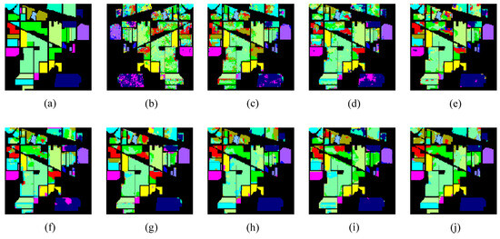
Figure 9. Indian Pines. (a) Ground-truth map. Classification results for different methods: (b) SVM; (c) 3-D-CNN; (d) DFSL; (e) DCFSL; (f) GIA-CFSL; (g) ADAFSL; (h) DMCM; (i) FDFSL; (j) our method.

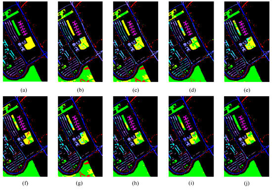
Figure 10. Pavia University. (a) Ground-truth map. Classification results for different methods: (b) SVM; (c) 3-D-CNN; (d) DFSL; (e) DCFSL; (f) GIA-CFSL; (g) ADAFSL; (h) DMCM; (i) FDFSL; (j) our method.

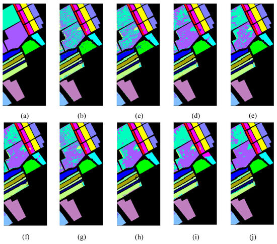
Figure 11. Salinas. (a) Ground-truth map. Classification results for different methods: (b) SVM; (c) 3-D-CNN; (d) DFSL; (e) DCFSL; (f) GIA-CFSL; (g) ADAFSL; (h) DMCM; (i) FDFSL; (j) our method.

4. Discussion

4.1. Learning Rate

When training a deep learning model, the learning rate is a key hyperparameter whose setting has a major influence on the model’s performance and pace of convergence. A reasonable learning rate can accelerate model convergence, and it assists the weights in rapidly approaching the global optimum. To find the optimal learning rate, as shown in Table 11, we explored the impact of different learning rate settings, including l × 10⁻⁵, l × 10⁻⁴, l × 10⁻³, l × 10⁻², and l × 10⁻¹, on model training. The model performed best in classification on the IP, PU, and SA datasets when the learning rate was set to l × 10⁻³, according to the experimental results. This suggests that, during optimization, a learning rate of l × 10⁻³ balances the convergence speed and stability, avoiding oscillations caused by a rate that is too large and overcoming slow convergence caused by a rate that is too small. Therefore, we ultimately selected 1 × 10⁻³ as the learning rate.

Table 11. Influence of different learning rates on model performance.

Target Data	l × 10−5	l × 10−4	l × 10−3	l × 10−2	l × 10−1
Pavia University	83.12	84.52	89.68	86.59	84.32
Indian Pines	73.03	76.67	81.23	77.70	73.99
Salinas	90.30	92.01	92.20	90.21	90.51

4.2. Comparison of Feature Extractor Modules

This section presents a comparative analysis of the efficient multi-scale dimensional feature fusion (EMDF) method’s influence on the classification accuracy of TD datasets. To validate the method’s effectiveness, we designed rigorous comparative experiments evaluating both the original framework and the improved framework, incorporating the EMDF method on three representative hyperspectral remote sensing datasets: Indian Pines (IP), Pavia University (PU), and Salinas Valley (SA). As shown in Figure 12, Figure 13 and Figure 14, a quantitative analysis demonstrates significant accuracy improvements across all three benchmark datasets after the EMDF method was implemented: the IP dataset achieved a 3.01% accuracy increase, PU improved by 2.55%, and SA showed a 1.59% enhancement. The experimental results confirm that the proposed EMDF method, through its unique cross-scale feature fusion mechanism, effectively integrates local detail features with global contextual information. This integration improves both the model’s classification accuracy and its ability to generalize across different datasets.

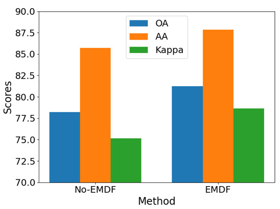
Figure 12. Feature extractor module comparison on Indian Pines.

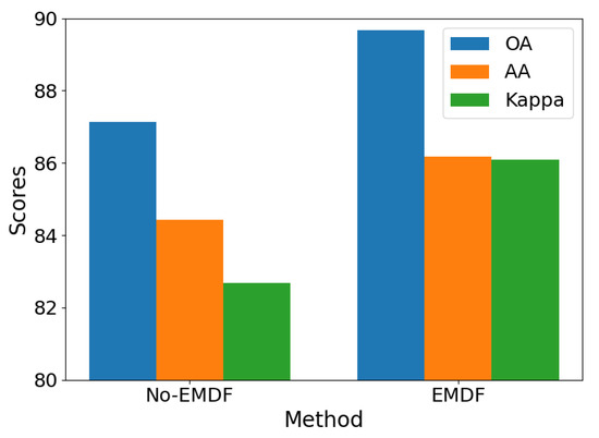
Figure 13. Feature extractor module comparison on Pavia University.

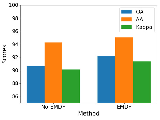
Figure 14. Feature extractor module comparison on Salines.

4.3. Different Numbers of Training Samples

The number of training samples greatly influences the model’s performance in cross-domain FSL. This subsection confirms the efficacy of our suggested framework by examining the precise effects of the amount of training samples on the performance of SVM, 3DCNN, DFSL, and cross-domain FSL techniques. As shown in Figure 15, Figure 16 and Figure 17, from the set 1, 2, 3, 4, 5, we chose at random how many labeled samples there were in each class. The findings of the experiment demonstrate that the classification accuracy and generalization capacity of each approach may be considerably enhanced by suitably expanding the number of training samples in TD. The model has a tendency to overfit when there are few training samples available; however, as the number of samples increases, the model can better learn class features, thereby improving classification accuracy. Notably, our suggested framework continuously outperformed all other approaches, irrespective of the quantity of training samples. This outcome clearly shows how successful our system is.

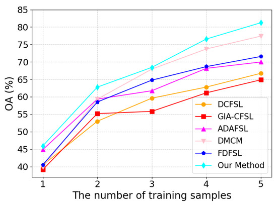
Figure 15. Impact of varying training sample sizes on the performance of various methods on Indian Pines.

Figure 16. Impact of varying training sample sizes on the performance of various methods on Pavia University.

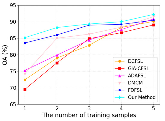
Figure 17. Impact of varying training sample sizes on the performance of various methods on Salines.

4.4. Computational Complexity

In order to thoroughly assess the computational effectiveness of various approaches, we conducted a systematic analysis of the computational complexity of deep learning approaches from four perspectives: training time, testing time, floating-point operations (FLOPs), and the number of parameters. In the comparative experiments, we focused on FSL (few-shot learning-based methods. To ensure fairness, every method was evaluated in several TD under uniform circumstances and trained on the same SD. As shown in Table 12, five labeled examples per class were employed in the experimental setting, and the majority of the testing time was devoted to predicting unlabeled samples from the HSI dataset, whereas the majority of the training time was devoted to the transfer learning procedure. Although our approach is not the best in terms of computational complexity, all metrics remain within acceptable ranges, demonstrating good computational efficiency.

Table 12. Training time, testing time, flops, and parameters on each dataset with different methods.

Datasets	Methods	DCFSL	GIA-CFSL	ADAFSL	DMCM	FDFSL	Our
Indians Pines	Training time	2289.96 s	3398.78 s	3994.02 s	5053.14 s	1167.07 s	4875.52 s
	Testing time	1.68 s	1.15 s	2.83 s	1.06 s	1.62 s	1.37 s
	Flops	0.0411 G	5.3325 G	0.0424 G	1.5423 G	0.5271 G	1.3080 G
	Parameters	0.0381 M	0.1851 M	0.0242 M	0.2654 M	0.1905 M	0.2529 M
Pavia University	Training time	1482.50 s	2245.34 s	1573.24 s	3241.75 s	769.34 s	3148.26 s
	Testing time	6.25 s	4.37 s	9.19 s	3.99 s	6.35 s	3.48 s
	Flops	0.0411 G	5.3325 G	0.0424 G	1.5423 G	0.5271 G	1.3080 G
	Parameters	0.0381 M	0.1851 M	0.0242 M	0.2634 M	0.1905 M	0.2529 M
Salinas	Training time	2283.42 s	5937.97 s	2458.48 s	5311.89 s	1225.49 s	4796.96 s
	Testing time	7.79 s	6.33 s	13.13 s	3.75 s	9.96 s	8.98 s
	Flops	0.0411 G	5.3325 G	0.0424 G	1.5423 G	0.5271 G	1.3080 G
	Parameters	0.0381 M	0.1851 M	0.0242 M	0.2654 M	0.1905 M	0.2529 M

5. Conclusions

This paper has introduced an innovative CDDW-CFSL framework designed to solve the issue of domain shift in HSIC. By integrating a multi-dimensional feature extraction module with a class-weighted domain adaptation method, the framework significantly enhances the adaptability and classification accuracy of cross-domain HSI. The multi-dimensional feature extraction module is capable of thoroughly excavating multi-level information within the images, including spatial, spectral, and textural features. Meanwhile, by dynamically modifying class weights, the class-weighted domain adaptation method successfully reduces the distribution disparity between SD and TD, demonstrating exceptional performance, especially in scenarios of class imbalance. The experimental results indicate that, compared to traditional domain adaptation methods, the CDDW-CFSL framework achieves notable performance improvements across multiple public datasets.

References

- Li, S.; Song, W.; Fang, L.; Chen, Y.; Ghamisi, P.; Benediktsson, J.A. Deep learning for hyperspectral image classification: An overview. IEEE Trans. Geosci. Remote Sens. 2019, 57, 6690–6709. [Google Scholar] [CrossRef]
- Zhang, Y.; Li, W.; Zhang, M.; Qu, Y.; Tao, R.; Qi, H. Topological structure and semantic information transfer network for cross-scene hyperspectral image classification. IEEE Trans. Neural Netw. Learn. Syst. 2021, 34, 2817–2830. [Google Scholar] [CrossRef]
- Zou, J.; He, W.; Zhang, H. Lessformer: Local-enhanced spectral-spatial transformer for hyperspectral image classification. IEEE Trans. Geosci. Remote Sens. 2022, 60, 5535416. [Google Scholar] [CrossRef]
- Liu, Y.; Sun, D.; Hu, X.; Ye, X.; Li, Y.; Liu, S.; Cao, K.; Chai, M.; Zhou, W.; Zhang, J. The advanced hyperspectral imager: Aboard China’s GaoFen-5 satellite. IEEE Geosci. Remote Sens. Mag. 2019, 7, 23–32. [Google Scholar] [CrossRef]
- Huang, Y.; Shen, Q.; Fu, Y.; You, S. Weakly-supervised semantic segmentation in cityscape via hyperspectral image. In Proceedings of the IEEE/CVF International Conference on Computer Vision (ICCV), Montreal, BC, Canada, 11–17 October 2021; pp. 1117–1126. [Google Scholar]
- Lu, J.; Liu, H.; Yao, Y.; Tao, S.; Tang, Z.; Lu, J. HSI road: A hyperspectral image dataset for road segmentation. In Proceedings of the 2020 IEEE International Conference on Multimedia and Expo (ICME), London, UK, 6–10 July 2020; pp. 1–6. [Google Scholar]
- Hong, D.; Gao, L.; Yao, J.; Zhang, B.; Plaza, A.; Chanussot, J. Graph convolutional networks for hyperspectral image classification. IEEE Trans. Geosci. Remote Sens. 2020, 59, 5966–5978. [Google Scholar] [CrossRef]
- Liu, J.; Feng, Q.; Liang, T.; Yin, J.; Gao, J.; Ge, J.; Hou, M.; Wu, C.; Li, W. Estimating the forage neutral detergent fiber content of Alpine grassland in the Tibetan Plateau using hyperspectral data and machine learning algorithms. IEEE Trans. Geosci. Remote Sens. 2021, 60, 1–17. [Google Scholar] [CrossRef]
- Dong, Y.; Liu, Q.; Du, B.; Zhang, L. Weighted feature fusion of convolutional neural network and graph attention network for hyperspectral image classification. IEEE Trans. Image Process. 2022, 31, 1559–1572. [Google Scholar] [CrossRef]
- Hong, D.; Han, Z.; Yao, J.; Gao, L.; Zhang, B.; Plaza, A.; Chanussot, J. SpectralFormer: Rethinking hyperspectral image classification with transformers. IEEE Trans. Geosci. Remote Sens. 2021, 60, 5518615. [Google Scholar] [CrossRef]
- Dong, Y.; Liang, T.; Yang, C.; Luo, H.; Zhang, Y. Joint distance transfer metric learning for remote-sensing image classification. IEEE Geosci. Remote Sens. Lett. 2022, 19, 6506205. [Google Scholar] [CrossRef]
- Su, Y.; Chen, J.; Gao, L.; Plaza, A.; Jiang, M.; Xu, X.; Sun, X.; Li, P. ACGT-Net: Adaptive cuckoo refinement-based graph transfer network for hyperspectral image classification. IEEE Trans. Geosci. Remote Sens. 2023, 61, 1–14. [Google Scholar] [CrossRef]
- Lu, S.; Zhang, M.; Huo, Y.; Wang, C.; Wang, J.; Gao, C. SSUM: Spatial—Spectral Unified Mamba for Hyperspectral Image Classification. Remote Sens. 2024, 16, 4653. [Google Scholar] [CrossRef]
- Shi, C.; Wu, H.; Wang, L. A positive feedback spatial–spectral correlation network based on spectral slice for hyperspectral image classification. IEEE Trans. Geosci. Remote Sens. 2023, 61, 5503417. [Google Scholar] [CrossRef]
- Zhang, L.; Zeng, Y.; Zhao, J.; Lan, J. A novel global–local block spatial–spectral fusion attention model for hyperspectral image classification. Remote Sens. Lett. 2022, 13, 343–351. [Google Scholar] [CrossRef]
- Ding, C.; Zheng, M.; Zheng, S.; Xu, Y.; Zhang, L.; Wei, W.; Zhang, Y. Integrating prototype learning with graph convolution network for effective active hyperspectral image classification. IEEE Trans. Geosci. Remote Sens. 2024, 62, 1–16. [Google Scholar] [CrossRef]
- Qu, J.; Zhang, L.; Dong, W.; Li, N.; Li, Y. Shared-Private Decoupling-Based Multilevel Feature Alignment Semi-Supervised Learning for HSI and LiDAR Classification. IEEE Trans. Geosci. Remote Sens. 2024; in press. [Google Scholar] [CrossRef]
- Manian, V.; Alfaro-Mejía, E.; Tokars, R.P. Hyperspectral image labeling and classification using an ensemble semi-supervised machine learning approach. Sensors 2022, 22, 1623. [Google Scholar] [CrossRef]
- Wang, Z.; Du, B. Unified active and semi-supervised learning for hyperspectral image classification. GeoInformatica 2023, 27, 23–38. [Google Scholar] [CrossRef]
- Cao, Z.; Li, X.; Feng, Y.; Chen, S.; Xia, C.; Zhao, L. ContrastNet: Unsupervised feature learning by autoencoder and prototypical contrastive learning for hyperspectral imagery classification. Neurocomputing 2021, 460, 71–83. [Google Scholar] [CrossRef]
- Sun, Y.; Liu, B.; Yu, X.; Yu, A.; Gao, K.; Ding, L. Perceiving spectral variation: Unsupervised spectrum motion feature learning for hyperspectral image classification. IEEE Trans. Geosci. Remote Sens. 2022, 60, 1–17. [Google Scholar] [CrossRef]
- Wei, W.; Xu, S.; Zhang, L.; Zhang, J.; Zhang, Y. Boosting hyperspectral image classification with unsupervised feature learning. IEEE Trans. Geosci. Remote Sens. 2021, 60, 5502315. [Google Scholar] [CrossRef]
- Yang, S.; Jia, Y.; Ding, Y.; Wu, X.; Hong, D. Unlabeled data guided partial label learning for hyperspectral image classification. IEEE Geosci. Remote Sens. Lett. 2024, 21, 5503405. [Google Scholar] [CrossRef]
- Zheng, X.; Jia, J.; Chen, J.; Guo, S.; Sun, L.; Zhou, C.; Wang, Y. Hyperspectral image classification with imbalanced data based on semi-supervised learning. Appl. Sci. 2022, 12, 3943. [Google Scholar] [CrossRef]
- Wang, Q.; Chen, M.; Zhang, J.; Kang, S.; Wang, Y. Improved active deep learning for semi-supervised classification of hyperspectral image. Remote Sens. 2021, 14, 171. [Google Scholar] [CrossRef]
- Zhang, S.; Xu, M.; Zhou, J.; Jia, S. Unsupervised spatial-spectral cnn-based feature learning for hyperspectral image classification. IEEE Trans. Geosci. Remote Sens. 2022, 60, 5524617. [Google Scholar] [CrossRef]
- Gao, K.; Liu, B.; Yu, X.; Zhang, P.; Tan, X.; Sun, Y. Small sample classification of hyperspectral image using model-agnostic meta-learning algorithm and convolutional neural network. Int. J. Remote Sens. 2021, 42, 3090–3122. [Google Scholar] [CrossRef]
- Wu, H.; Li, M.; Wang, A. A novel meta-learning-based hyperspectral image classification algorithm. Front. Phys. 2023, 11, 1163555. [Google Scholar] [CrossRef]
- Zhang, J.; Liu, L.; Zhao, R.; Shi, Z. A Bayesian meta-learning-based method for few-shot hyperspectral image classification. IEEE Trans. Geosci. Remote Sens. 2022, 61, 1–13. [Google Scholar] [CrossRef]
- Wang, Y.; Liu, M.; Yang, Y.; Li, Z.; Du, Q.; Chen, Y.; Li, F.; Yang, H. Heterogeneous few-shot learning for hyperspectral image classification. IEEE Geosci. Remote Sens. Lett. 2021, 19, 5510405. [Google Scholar] [CrossRef]
- Yuan, H.; Huang, K.; Duan, J.; Lai, L.; Yu, J.; Huang, C.; Yang, Z. Generalized few-shot learning for crop hyperspectral image precise classification. Comput. Electron. Agric. 2024, 227, 109498. [Google Scholar] [CrossRef]
- Zhao, Y.; Sun, J.; Hu, N.; Zai, C.; Han, Y. Residual channel attention based sample adaptation few-shot learning for hyperspectral image classification. Sci. Rep. 2024, 14, 26746. [Google Scholar] [CrossRef]
- Xiao, F.; Xiang, H.; Cao, C.; Gao, X. Neural architecture search-based few-shot learning for hyperspectral image classification. IEEE Trans. Geosci. Remote Sens. 2024, 62, 5513715. [Google Scholar] [CrossRef]
- Zhao, Y.; Sun, J.; Zai, C.; Han, Y.; Hu, N. Attention-Based Sample Adaptation Few-Shot Learning for Hyperspectral Image Classification. Res. Sq. 2024. [Google Scholar] [CrossRef]
- Liu, B.; Yu, X.; Yu, A.; Zhang, P.; Wan, G.; Wang, R. Deep few-shot learning for hyperspectral image classification. IEEE Trans. Geosci. Remote Sens. 2018, 57, 2290–2304. [Google Scholar] [CrossRef]
- Xi, B.; Li, J.; Li, Y.; Song, R.; Hong, D.; Chanussot, J. Few-shot learning with class-covariance metric for hyperspectral image classification. IEEE Trans. Image Process. 2022, 31, 5079–5092. [Google Scholar] [CrossRef]
- Tang, H.; Zhang, C.; Tang, D.; Lin, X.; Yang, X.; Xie, W. Few-Shot Hyperspectral Image Classification with Deep Fuzzy Metric Learning. IEEE Geosci. Remote Sens. Lett. 2025. [Google Scholar] [CrossRef]
- Li, X.; Yang, X.; Ma, Z.; Xue, J. Deep metric learning for few-shot image classification: A review of recent developments. Pattern Recognit. 2023, 138, 109381. [Google Scholar] [CrossRef]
- Liu, Y.; Zhang, H.; Zhang, W.; Lu, G.; Tian, Q.; Ling, N. Few-shot image classification: Current status and research trends. Electronics 2022, 11, 1752. [Google Scholar] [CrossRef]
- Xin, Z.; Wang, L.; Xu, M.; Li, Z. Hyperspectral image few-shot classification network with Brownian distance covariance. IEEE Geosci. Remote Sens. Lett. 2023, 20, 1–5. [Google Scholar] [CrossRef]
- Bai, J.; Huang, S.; Xiao, Z.; Li, X.; Zhu, Y.; Regan, A.C.; Jiao, L. Few-shot hyperspectral image classification based on adaptive subspaces and feature transformation. IEEE Trans. Geosci. Remote Sens. 2022, 60, 1–17. [Google Scholar] [CrossRef]
- Wang, S.; Wang, B.; Zhang, Z.; Heidari, A.A.; Chen, H. Class-aware sample reweighting optimal transport for multi-source domain adaptation. Neurocomputing 2023, 523, 213–223. [Google Scholar] [CrossRef]
- Li, Y.; Guo, L.; Ge, Y. Pseudo labels for unsupervised domain adaptation: A review. Electronics 2023, 12, 3325. [Google Scholar] [CrossRef]
- Li, Z.; Liu, M.; Chen, Y.; Xu, Y.; Li, W.; Du, Q. Deep Cross-Domain Few-Shot Learning for Hyperspectral Image Classification. IEEE Trans. Geosci. Remote Sens. 2022, 60, 1–18. [Google Scholar] [CrossRef]
- Hu, L.; He, W.; Zhang, L.; Zhang, H. Cross-domain meta-learning under dual-adjustment mode for few-shot hyperspectral image classification. IEEE Trans. Geosci. Remote Sens. 2023, 61, 1–16. [Google Scholar] [CrossRef]
- Zhang, Y.; Li, W.; Zhang, M.; Wang, S.; Tao, R.; Du, Q. Graph information aggregation cross-domain few-shot learning for hyperspectral image classification. IEEE Trans. Neural Netw. Learn. Syst. 2022, 35, 1912–1925. [Google Scholar] [CrossRef]
- Qin, B.; Feng, S.; Zhao, C.; Li, W.; Tao, R.; Xiang, W. Cross-domain few-shot learning based on feature disentanglement for hyperspectral image classification. IEEE Trans. Geosci. Remote Sens. 2024. [Google Scholar] [CrossRef]
- Luo, Y.; Zheng, L.; Guan, T.; Yu, J.; Yang, Y. Taking a closer look at domain shift: Category-level adversaries for semantics consistent domain adaptation. In Proceedings of the IEEE/CVF Conference on Computer Vision and Pattern Recognition (CVPR), Long Beach, CA, USA, 15–19 June 2019; pp. 2507–2516. [Google Scholar]
- Li, Y.; Li, Z.; Su, A.; Wang, K.; Wang, Z.; Yu, Q. Semi-supervised Cross-domain Remote Sensing Scene Classification via Category-level Feature Alignment Network. IEEE Trans. Geosci. Remote Sens. 2024, 62, 1–15. [Google Scholar] [CrossRef]
- Xue, J.; Zhao, Y.; Wu, T.; Wang, H.; Liu, Q. Tensor Convolution-Like Low-Rank Dictionary for High-Dimensional Image Representation. IEEE Trans. Circuits Syst. Video Technol. 2024, 34, 13257–13270. [Google Scholar] [CrossRef]
- Ye, Z.; Wang, J.; Liu, H.; Zhang, Y.; Li, W. Adaptive domain-adversarial few-shot learning for cross-domain hyperspectral image classification. IEEE Trans. Geosci. Remote Sens. 2023, 61, 5532017. [Google Scholar] [CrossRef]
- Feng, J.; Zhou, Z.; Shang, R.; Wu, J.; Zhang, T.; Zhang, X.; Jiao, L. Class-aligned and class-balancing generative domain adaptation for hyperspectral image classification. IEEE Trans. Geosci. Remote Sens. 2024, 62, 5509617. [Google Scholar] [CrossRef]
- Ding, C.; Deng, Z.; Xu, Y.; Zheng, M.; Zhang, L.; Cao, Y.; Wei, W.; Zhang, Y. GLGAT-CFSL: Global-Local Graph Attention Networks Based Cross-Domain Few-Shot Learning for Hyperspectral Image Classification. IEEE Trans. Geosci. Remote Sens. 2024, 62, 1–19. [Google Scholar] [CrossRef]
Disclaimer/Publisher’s Note: The statements, opinions and data contained in all publications are solely those of the individual author(s) and contributor(s) and not of MDPI and/or the editor(s). MDPI and/or the editor(s) disclaim responsibility for any injury to people or property resulting from any ideas, methods, instructions or products referred to in the content. |
© 2025 by the authors. Licensee MDPI, Basel, Switzerland. This article is an open access article distributed under the terms and conditions of the Creative Commons Attribution (CC BY) license (https://creativecommons.org/licenses/by/4.0/).