
Mooring Observations of Typhoon Trami (2024)-Induced Upper-Ocean Variability: Diapycnal Mixing and Internal Wave Energy Characteristics

Abstract
1. Introduction
2. Materials and Methods
2.1. Data
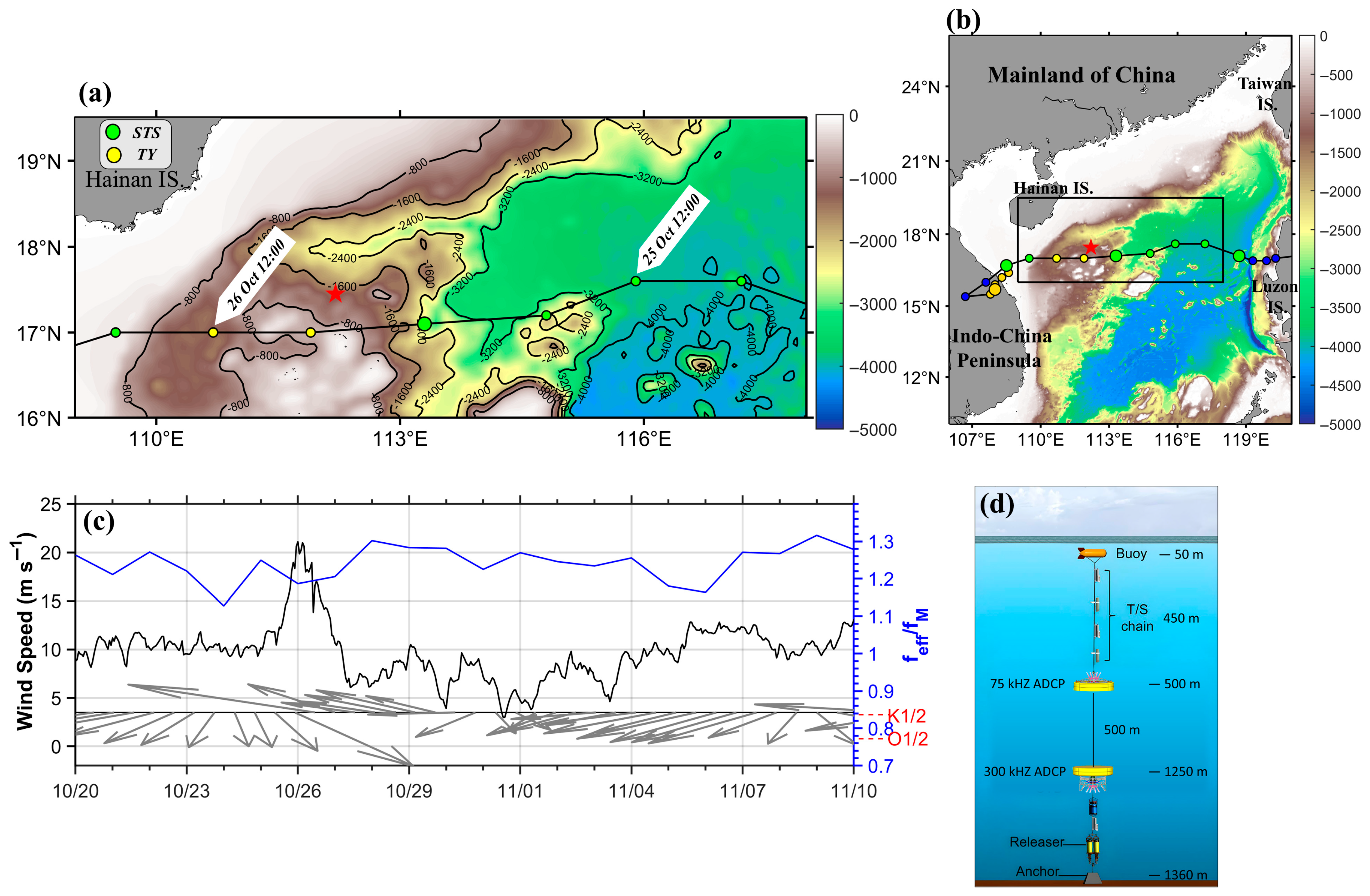
2.1.1. Mooring
2.1.2. TC Best Track and Wind Data
2.1.3. Satellite
2.2. Methods
2.2.1. Stability and Energy Estimates
2.2.2. Energy Transfer Rate
3. Results
3.1. Upper Ocean Thermal and Dynamical Response
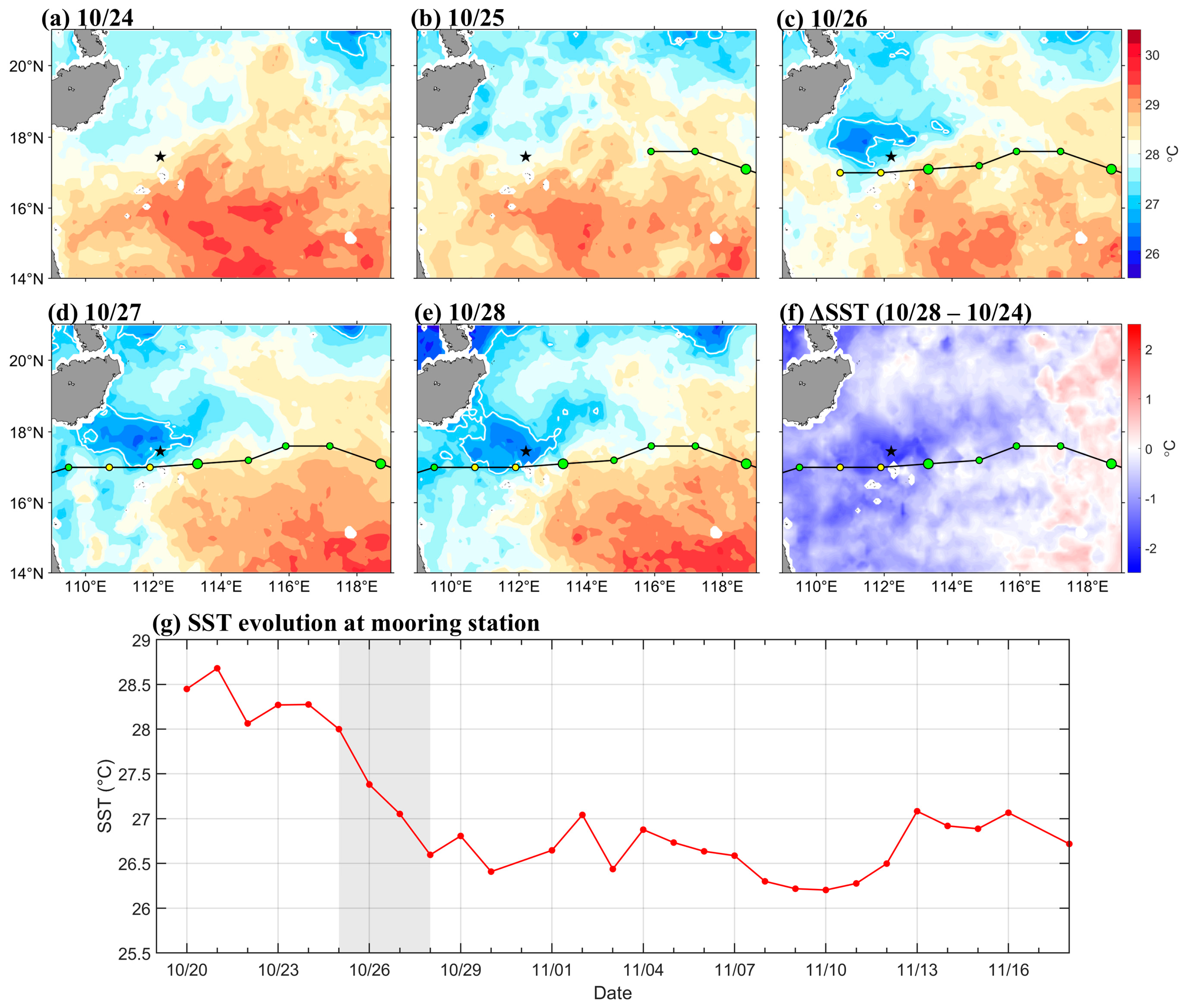
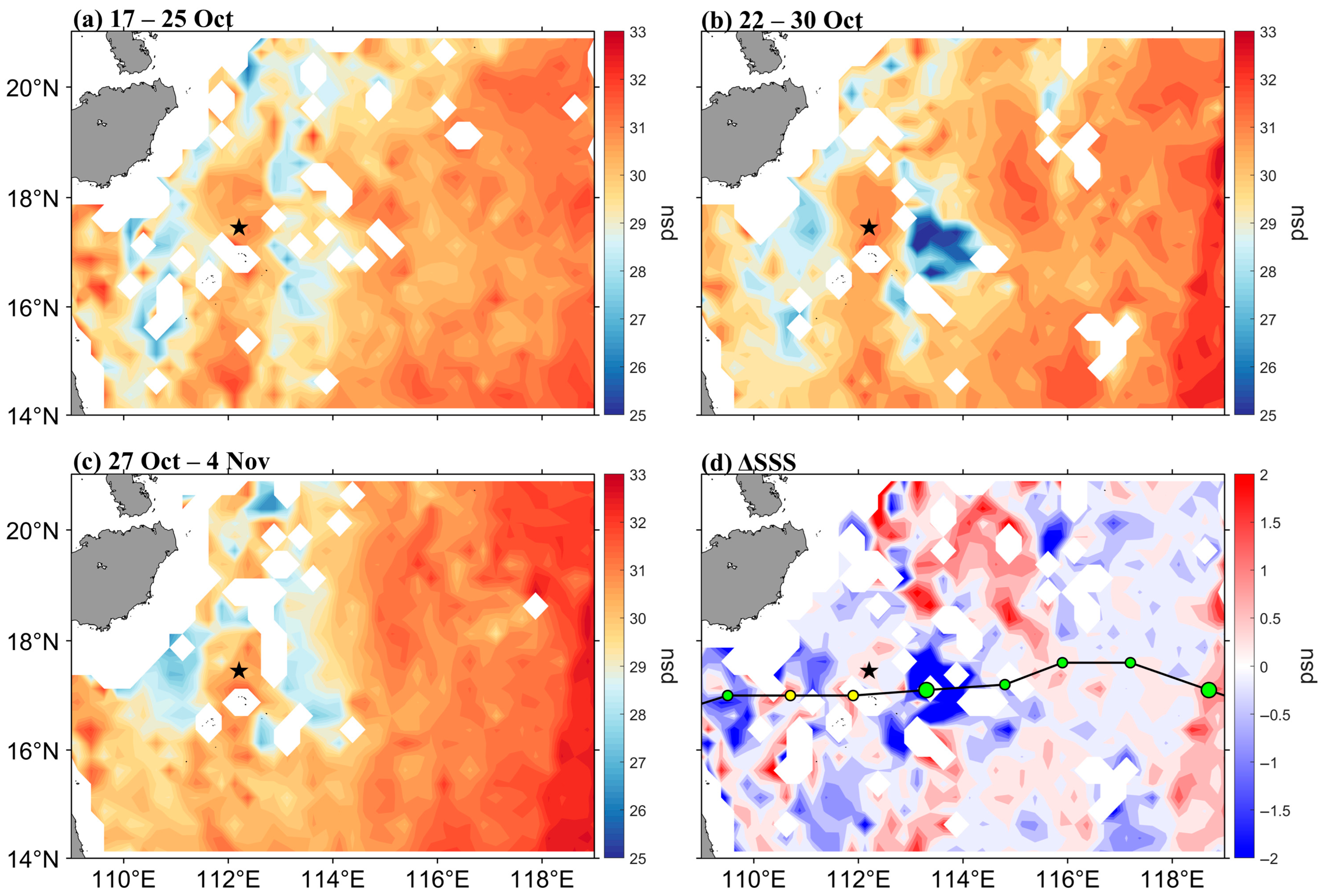
3.1.1. Satellite-Observed Sea Surface Response
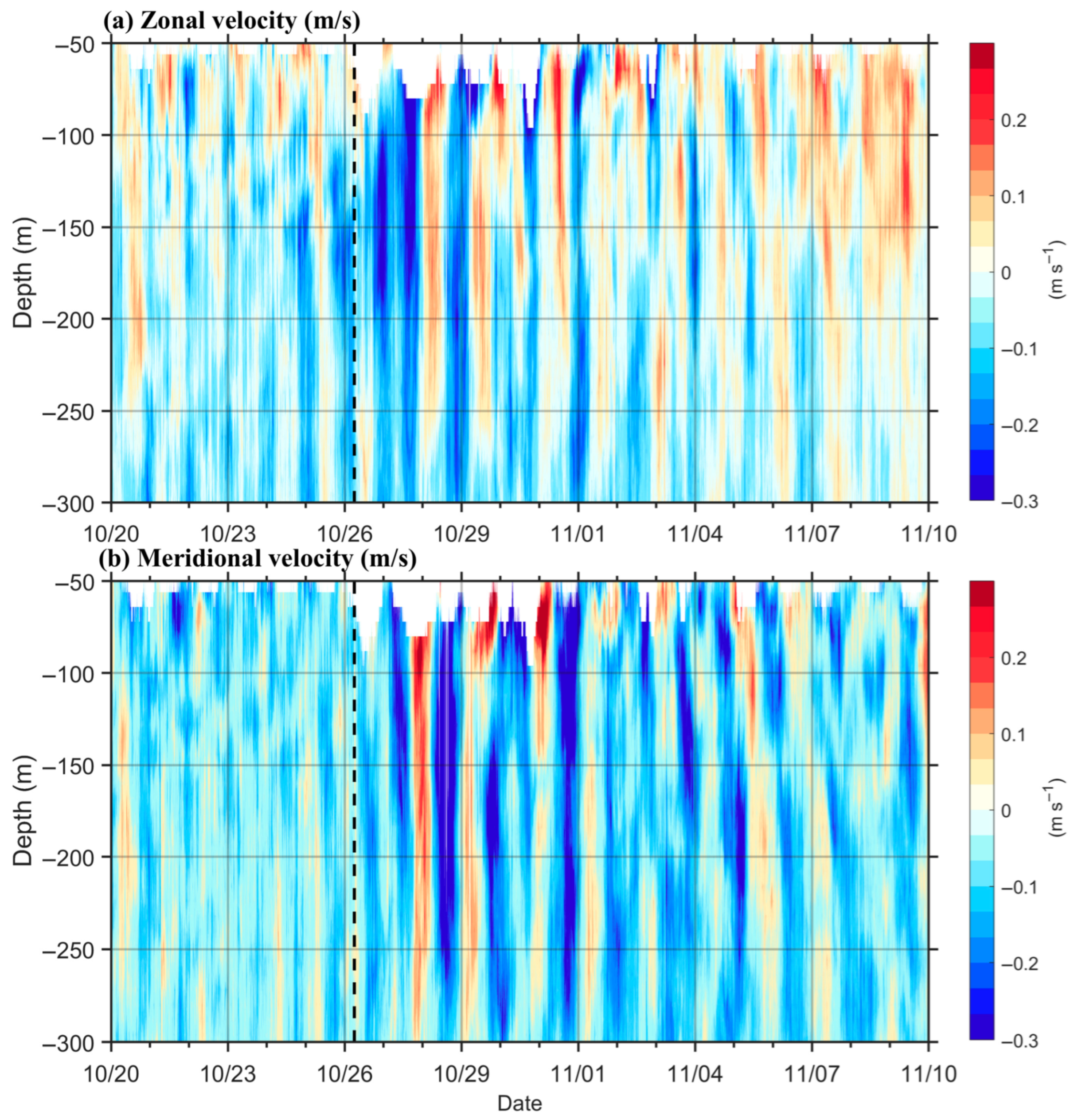
3.1.2. Mooring-Observed Subsurface Response
3.2. The Mixing Processes and Driving Factors of the Upper Ocean
3.2.1. Enhanced Diapycnal Mixing in the Upper Ocean Following the Typhoon
3.2.2. Contribution of NIWs to the Upper Ocean Shear Instability
3.3. Characteristics of Internal Wave Energy Distribution
3.3.1. The Temporal Evolution of NIW Kinetic Energy
3.3.2. Decomposition of Near-Inertial Energy
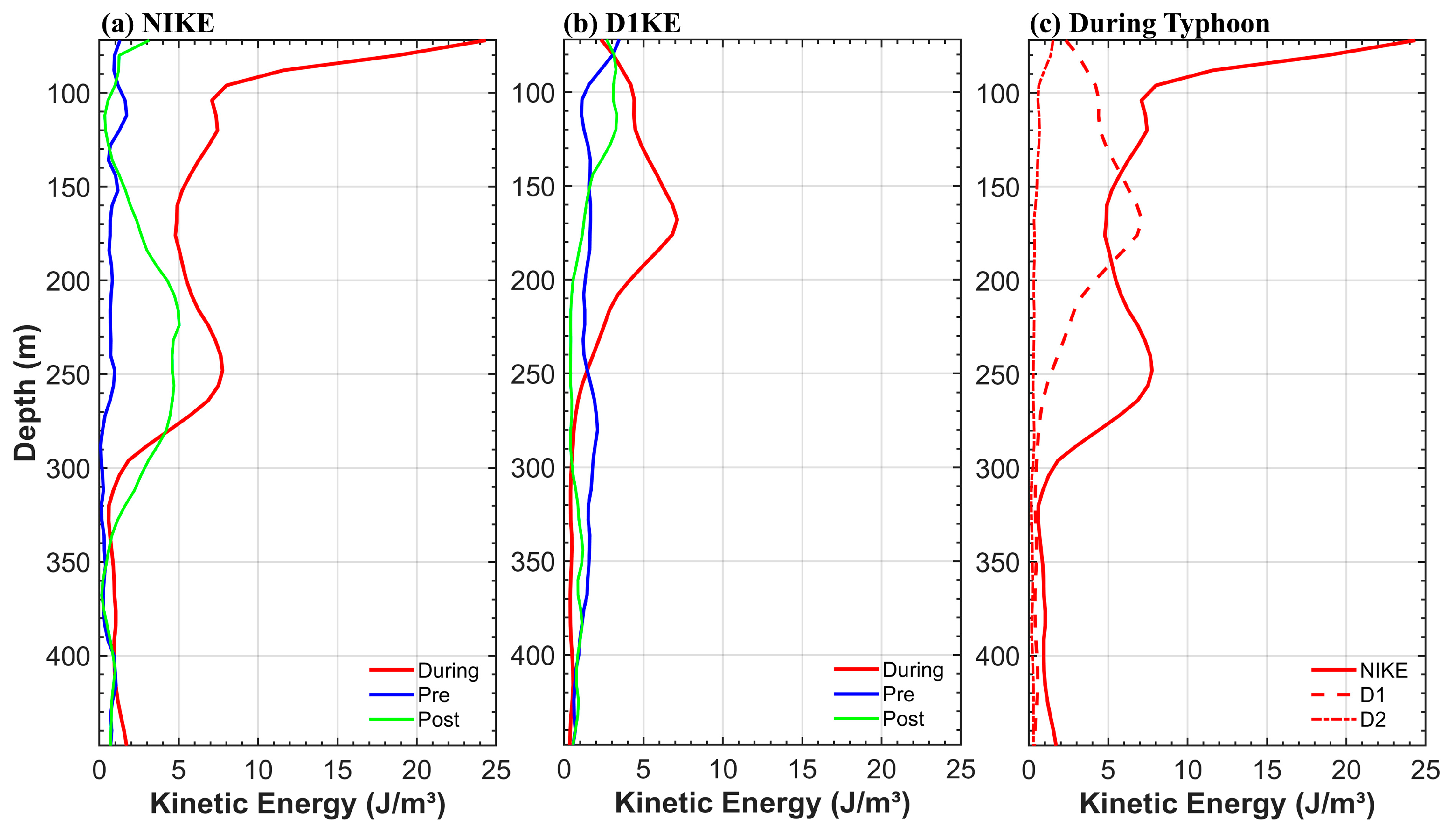
3.3.3. Depth Profiles of Time-Averaged Internal Wave Kinetic Energy
3.4. Burst of Subsurface-Layer Diurnal Tidal Energy
3.4.1. The Modulation of Stratification Change
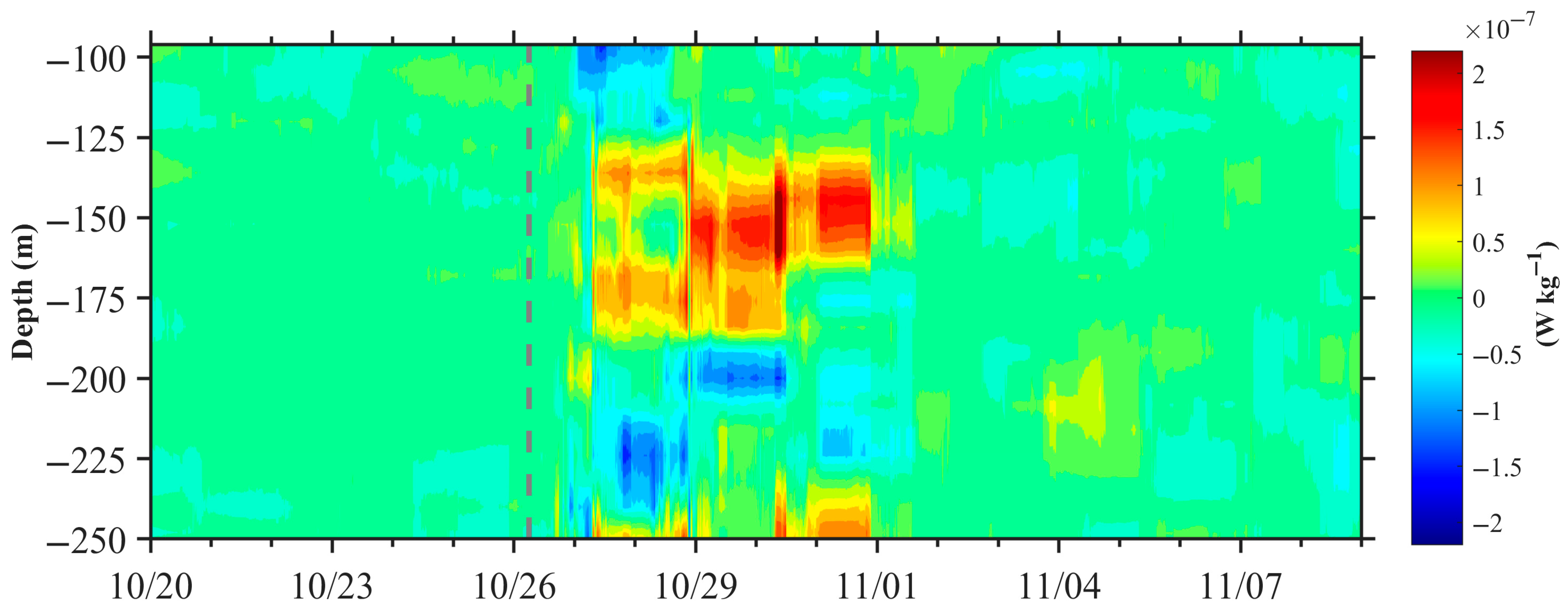
3.4.2. Energy Transfer from NIWs to D1 ITs
4. Discussion and Conclusions
- (1)
- Thermal and dynamical ocean response: Relying on multi-source satellite remote sensing SST and SSS data, it was found that the typhoon generated a “cold wake” with a maximum temperature decline of 2.5 °C and an approximate 0.5 psu increase in salinity to the right of the typhoon’s trajectory near the mooring site. This suggests that turbulent mixing took place in the upper ocean at the mooring location. The mooring data indicate that the maximum temperature drop of 4 °C occurred on 28 October, coinciding with the deepening of the mixed layer and the rise in the thermocline. Also, due to the influence of strong near-inertial oscillations introduced by the typhoon in the upper layer, the temperature changes also showed near-inertial periodicity.
- (2)
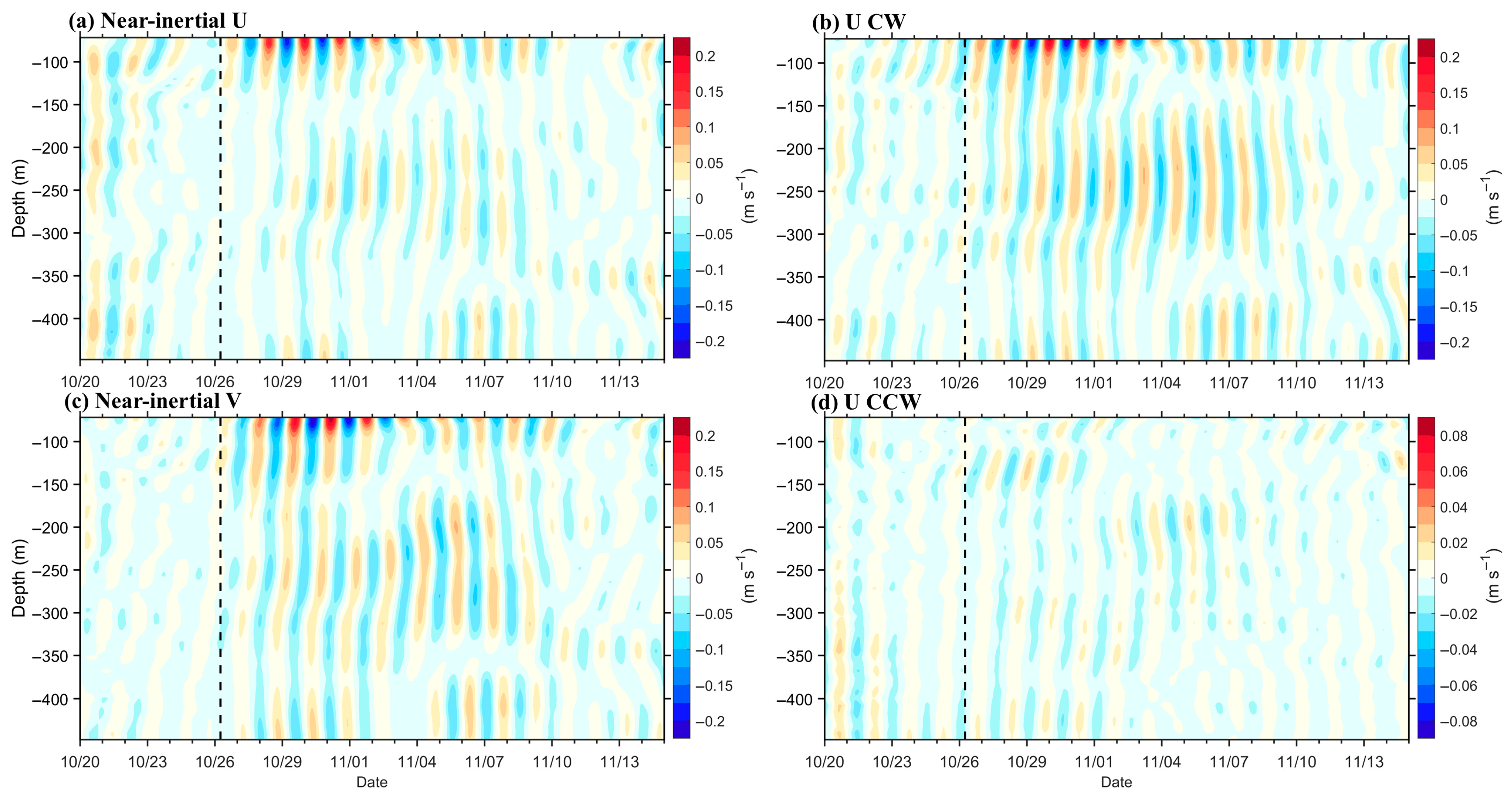
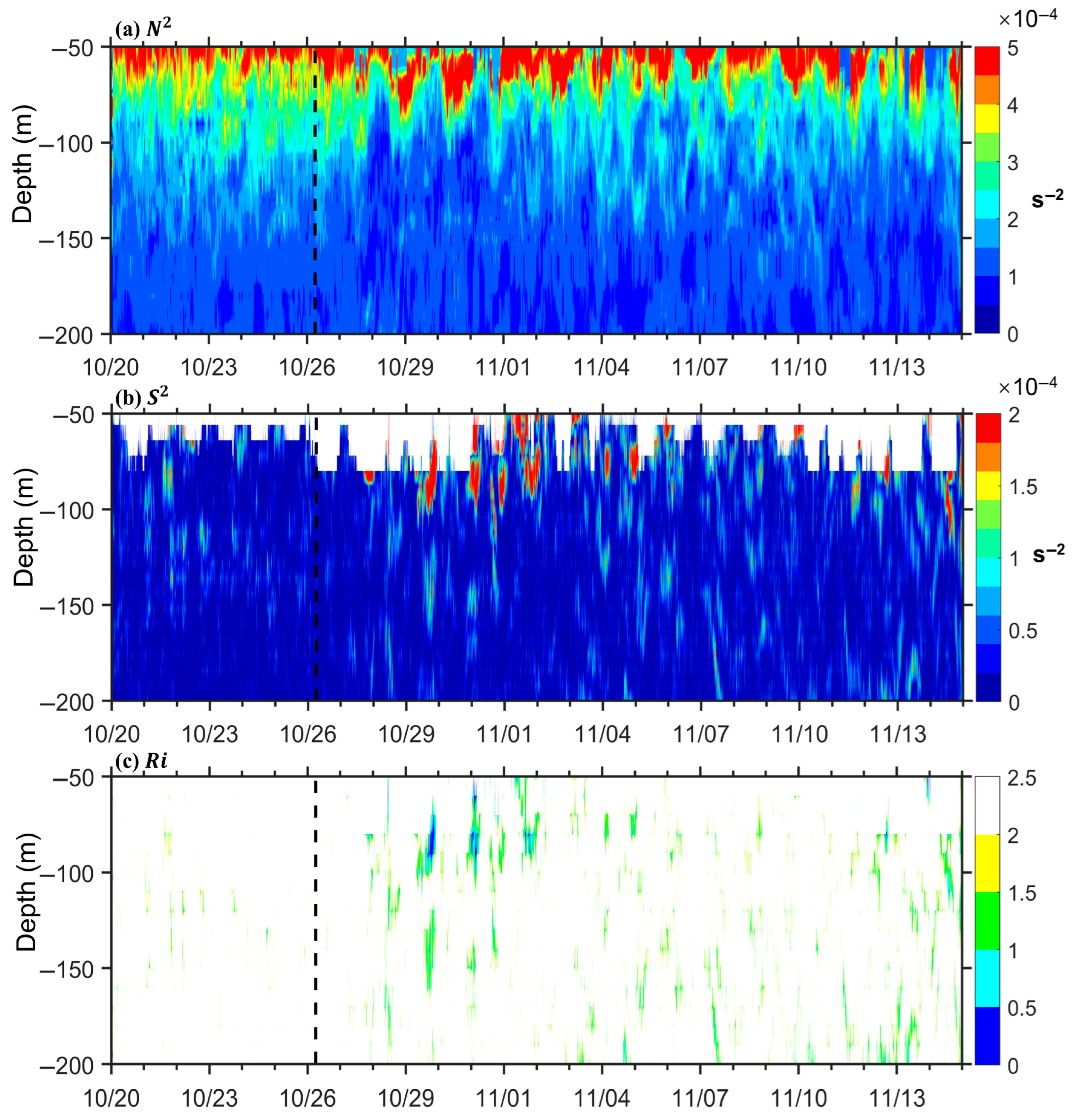
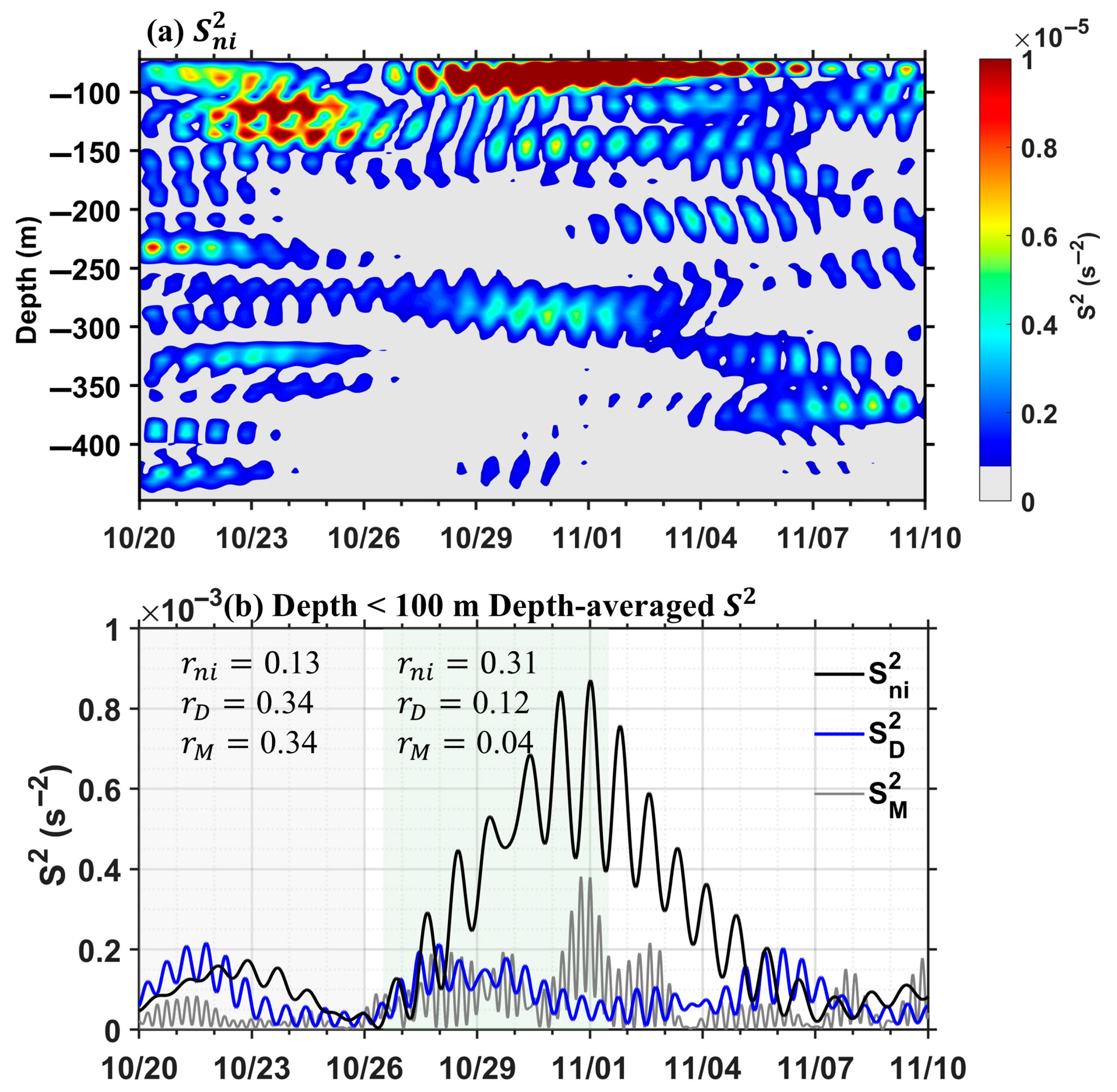
- Near-surface mixing process and its driving factors: Intense near-inertial internal waves induced significant near-inertial shear instability in the upper ocean, with peak shear squared persisting for about 9 days in our case. Moreover, the disruption of stratification collectively led to the occurrence of enhanced turbulence dissipation in the upper layer. Further analysis indicates that near-inertial shear was the primary factor responsible for the rapid increase in shear instability in the upper ocean, in contrast to the shear caused by pre-existing diurnal and semidiurnal internal tides.
- (3)
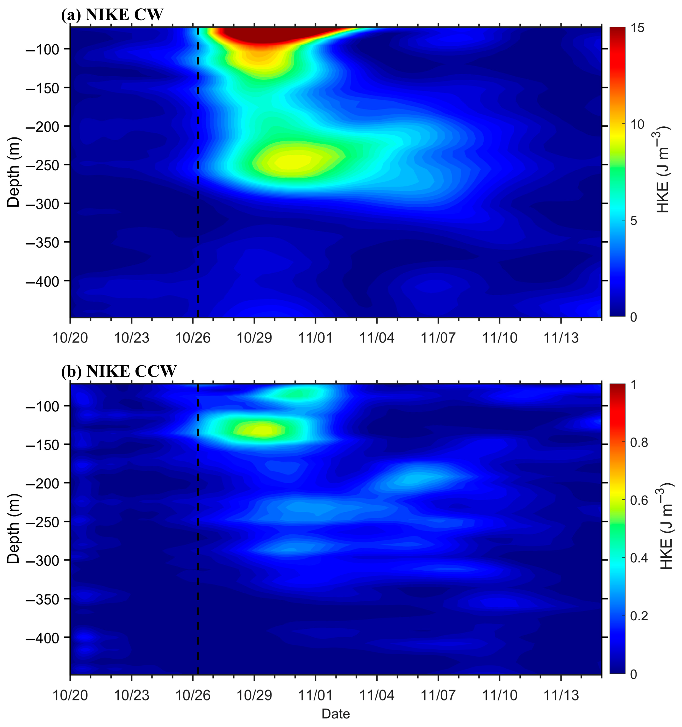
- Subsurface diurnal tidal energy enhancement: The study also investigated the characteristics of internal tidal energy distribution. Interestingly, it was found that near-inertial energy and diurnal tidal energy exhibited an inverse relationship in the subsurface layer between 120 and 170 m. Specifically, near-inertial energy hit a low at 170 m, while diurnal tidal energy peaked unexpectedly at that same depth. We further excluded both the effects of spring-neap tide and the changes in stratification on diurnal tidal energy distribution, and quantitatively assessed the energy transfer rate from near-inertial energy to diurnal tidal energy. The analysis revealed a notable rate of energy transfer from NIWs to D1 ITs within the 120–170 m depth range, peaking at 2 × 10⁻⁷ W kg−1. This is consistent with previous observations of energy transfer from low- to high-frequency internal waves. For example, mooring-based observations during Typhoon Fitow (2013) showed that M1 subharmonics and NIWs facilitated energy transfer to high-frequency internal waves (HFIWs) at a rate of 2 × 10⁻⁶ W kg−1 [42]. Similar magnitudes of energy transfer have been documented: 2 × 10⁻⁷ W kg−1 at the shelf break in the East China Sea [43], while open-ocean measurements indicate weaker transfer rates (3.7 × 10⁻⁹ W kg−1) [70].
Author Contributions
Funding
Institutional Review Board Statement
Informed Consent Statement
Data Availability Statement
Acknowledgments
Conflicts of Interest
References
- Wang, G.; Su, J.; Ding, Y.; Chen, D. Tropical Cyclone Genesis over the South China Sea. J. Mar. Syst. 2007, 68, 318–326. [Google Scholar] [CrossRef]
- Price, J.F. Upper Ocean Response to a Hurricane. J. Phys. Oceanogr. 1981, 11, 153–175. [Google Scholar] [CrossRef]
- Price, J.F.; Weller, R.A.; Pinkel, R. Diurnal Cycling: Observations and Models of the Upper Ocean Response to Diurnal Heating, Cooling, and Wind Mixing. J. Geophys. Res. 1986, 91, 8411–8427. [Google Scholar] [CrossRef]
- Zhu, T.; Zhang, D.-L. The Impact of the Storm-Induced SST Cooling on Hurricane Intensity. Adv. Atmos. Sci. 2006, 23, 14–22. [Google Scholar] [CrossRef]
- Zhang, H.; Xie, X.; Yang, C.; Qi, Y.; Tian, D.; Xu, J.; Cai, S.; Wu, R.; Ma, Y.; Ni, X.; et al. Observed Impact of Typhoon Mangkhut (2018) on a Continental Slope in the South China Sea. J. Geophys. Res. Ocean. 2022, 127, e2022JC018432. [Google Scholar] [CrossRef]
- Guan, S.; Zhao, W.; Huthnance, J.; Tian, J.; Wang, J. Observed Upper Ocean Response to Typhoon Megi (2010) in the Northern South China Sea. J. Geophys. Res. Ocean. 2014, 119, 3134–3157. [Google Scholar] [CrossRef]
- Zhang, H.; Wu, R.; Chen, D.; Liu, X.; He, H.; Tang, Y.; Ke, D.; Shen, Z.; Li, J.; Xie, J.; et al. Net Modulation of Upper Ocean Thermal Structure by Typhoon Kalmaegi (2014). J. Geophys. Res. Ocean. 2018, 123, 7154–7171. [Google Scholar] [CrossRef]
- Zhang, H.; Chen, D.; Zhou, L.; Liu, X.; Ding, T.; Zhou, B. Upper Ocean Response to Typhoon Kalmaegi (2014). J. Geophys. Res. Ocean. 2016, 121, 6520–6535. [Google Scholar] [CrossRef]
- Sanford, T.B.; Price, J.F.; Girton, J.B. Upper-Ocean Response to Hurricane Frances (2004) Observed by Profiling EM-APEX Floats. J. Phys. Oceanogr. 2011, 41, 1041–1056. [Google Scholar] [CrossRef]
- Wang, G.; Wu, L.; Johnson, N.C.; Ling, Z. Observed Three-dimensional Structure of Ocean Cooling Induced by Pacific Tropical Cyclones. Geophys. Res. Lett. 2016, 43, 7632–7638. [Google Scholar] [CrossRef]
- Lin, I.-I.; Liu, W.T.; Wu, C.-C.; Chiang, J.C.H.; Sui, C.-H. Satellite Observations of Modulation of Surface Winds by Typhoon-Induced Upper Ocean Cooling. Geophys. Res. Lett. 2003, 30, 1311. [Google Scholar] [CrossRef]
- Zhang, H.; He, H.; Zhang, W.-Z.; Tian, D. Upper Ocean Response to Tropical Cyclones: A Review. Geosci. Lett. 2021, 8, 1. [Google Scholar] [CrossRef]
- Ma, Z.; Zhang, Y.; Wu, R.; Na, R. Statistical Characteristics of the Response of Sea Surface Temperatures to Westward Typhoons in the South China Sea. Remote Sens. 2021, 13, 916. [Google Scholar] [CrossRef]
- D’Asaro, E.A.; Sanford, T.B.; Niiler, P.P.; Terrill, E.J. Cold Wake of Hurricane Frances. Geophys. Res. Lett. 2007, 34, 2007GL030160. [Google Scholar] [CrossRef]
- Glenn, S.M.; Miles, T.N.; Seroka, G.N.; Xu, Y.; Forney, R.K.; Yu, F.; Roarty, H.; Schofield, O.; Kohut, J. Stratified Coastal Ocean Interactions with Tropical Cyclones. Nat. Commun. 2016, 7, 10887. [Google Scholar] [CrossRef] [PubMed]
- Seroka, G.; Miles, T.; Xu, Y.; Kohut, J.; Schofield, O.; Glenn, S. Rapid Shelf-Wide Cooling Response of a Stratified Coastal Ocean to Hurricanes: Stratified Coastal Ocean Cooling in TCs. J. Geophys. Res. Ocean. 2017, 122, 4845–4867. [Google Scholar] [CrossRef] [PubMed]
- Grodsky, S.A.; Reul, N.; Lagerloef, G.; Reverdin, G.; Carton, J.A.; Chapron, B.; Quilfen, Y.; Kudryavtsev, V.N.; Kao, H. Haline Hurricane Wake in the Amazon/Orinoco Plume: AQUARIUS/SACD and SMOS Observations. Geophys. Res. Lett. 2012, 39, 2012GL053335. [Google Scholar] [CrossRef]
- Neetu, S.; Lengaigne, M.; Vincent, E.M.; Vialard, J.; Madec, G.; Samson, G.; Ramesh Kumar, M.R.; Durand, F. Influence of Upper-ocean Stratification on Tropical Cyclone-induced Surface Cooling in the Bay of Bengal. J. Geophys. Res. 2012, 117, 2012JC008433. [Google Scholar] [CrossRef]
- Chacko, N. Insights into the Haline Variability Induced by Cyclone Vardah in the Bay of Bengal Using SMAP Salinity Observations. Remote Sens. Lett. 2018, 9, 1205–1213. [Google Scholar] [CrossRef]
- Lu, Z.; Wang, G.; Shang, X. Inner-Core Sea Surface Cooling Induced by a Tropical Cyclone. J. Phys. Oceanogr. 2021, 51, 3385–3400. [Google Scholar] [CrossRef]
- Price, J.F.; Sanford, T.B.; Forristall, G.Z. Forced Stage Response to a Moving Hurricane. J. Phys. Oceanogr. 1994, 24, 233–260. [Google Scholar] [CrossRef]
- Sanford, T.B.; Price, J.F.; Girton, J.B.; Webb, D.C. Highly Resolved Observations and Simulations of the Ocean Response to a Hurricane. Geophys. Res. Lett. 2007, 34, L13604. [Google Scholar] [CrossRef]
- Teague, W.J.; Jarosz, E.; Wang, D.W.; Mitchell, D.A. Observed Oceanic Response over the Upper Continental Slope and Outer Shelf during Hurricane Ivan. J. Phys. Oceanogr. 2007, 37, 2181–2206. [Google Scholar] [CrossRef]
- Chen, G.; Xue, H.; Wang, D.; Xie, Q. Observed Near-Inertial Kinetic Energy in the Northwestern South China Sea. J. Geophys. Res. Ocean. 2013, 118, 4965–4977. [Google Scholar] [CrossRef]
- Alford, M.H. Improved Global Maps and 54-Year History of Wind-Work on Ocean Inertial Motions. Geophys. Res. Lett. 2003, 30, 1424. [Google Scholar] [CrossRef]
- D’Asaro, E.A. The Energy Flux from the Wind to Near-Inertial Motions in the Surface Mixed Layer. J. Phys. Ocean. 1985, 15, 1043–1059. [Google Scholar] [CrossRef]
- Jaimes, B.; Shay, L.K. Near-Inertial Wave Wake of Hurricanes Katrina and Rita over Mesoscale Oceanic Eddies. J. Phys. Oceanogr. 2010, 40, 1320–1337. [Google Scholar] [CrossRef]
- Cao, A.; Guo, Z.; Song, J.; Lv, X.; He, H.; Fan, W. Near-Inertial Waves and Their Underlying Mechanisms Based on the South China Sea Internal Wave Experiment (2010–2011). J. Geophys. Res. Ocean. 2018, 123, 5026–5040. [Google Scholar] [CrossRef]
- Gill, A.E. On the Behavior of Internal Waves in the Wakes of Storms. J. Phys. Oceanogr. 1984, 14, 1129–1151. [Google Scholar] [CrossRef]
- Whalen, C.B.; De Lavergne, C.; Naveira Garabato, A.C.; Klymak, J.M.; MacKinnon, J.A.; Sheen, K.L. Internal Wave-Driven Mixing: Governing Processes and Consequences for Climate. Nat. Rev. Earth Environ. 2020, 1, 606–621. [Google Scholar] [CrossRef]
- Alford, M.H. Redistribution of Energy Available for Ocean Mixing by Long-Range Propagation of Internal Waves. Nature 2003, 423, 159–162. [Google Scholar] [CrossRef] [PubMed]
- Simmons, H.L. Spectral Modification and Geographic Redistribution of the Semi-Diurnal Internal Tide. Ocean Model. 2008, 21, 126–138. [Google Scholar] [CrossRef]
- Xing, J.; Davies, A.M. Processes Influencing the Non-Linear Interaction between Inertial Oscillations, near Inertial Internal Waves and Internal Tides. Geophys. Res. Lett. 2002, 29, 11-1–11-14. [Google Scholar] [CrossRef]
- Zhang, S.; Chen, Z.; Wang, H.; Xu, J.; Zhang, Q.; Sun, Y.; Gong, Y.; Cai, S. A Numerical Study on Energy Transfer between Near-Inertial Internal Waves and Super-Inertial Internal Waves in the South China Sea under the Influence of a Typhoon. Cont. Shelf Res. 2024, 276, 105240. [Google Scholar] [CrossRef]
- Hu, Q.; Huang, X.; Xu, Q.; Zhou, C.; Guan, S.; Xu, X.; Zhao, W.; Yang, Q.; Tian, J. Parametric Subharmonic Instability of Diurnal Internal Tides in the Abyssal South China Sea. J. Phys. Oceanogr. 2023, 53, 195–213. [Google Scholar] [CrossRef]
- Jing, Z.; Chang, P.; DiMarco, S.F.; Wu, L. Role of Near-Inertial Internal Waves in Subthermocline Diapycnal Mixing in the Northern Gulf of Mexico. J. Phys. Oceanogr. 2015, 45, 3137–3154. [Google Scholar] [CrossRef]
- Xie, X.-H.; Shang, X.-D.; van Haren, H.; Chen, G.-Y.; Zhang, Y.-Z. Observations of Parametric Subharmonic Instability-Induced near-Inertial Waves Equatorward of the Critical Diurnal Latitude. Geophys. Res. Lett. 2011, 38, L05606. [Google Scholar] [CrossRef]
- Yang, W.; Hibiya, T.; Tanaka, Y.; Zhao, L.; Wei, H. Modification of Parametric Subharmonic Instability in the Presence of Background Geostrophic Currents. Geophys. Res. Lett. 2018, 45, 12957–12962. [Google Scholar] [CrossRef]
- Yang, W.; Wei, H.; Zhao, L. Parametric Subharmonic Instability of the Semidiurnal Internal Tides at the East China Sea Shelf Slope. J. Phys. Oceanogr. 2020, 50, 907–920. [Google Scholar] [CrossRef]
- Jing, Z.; Chang, P. Modulation of Small-Scale Superinertial Internal Waves by Near-Inertial Internal Waves. J. Phys. Oceanogr. 2016, 46, 3529–3548. [Google Scholar] [CrossRef]
- Sun, O.M.; Pinkel, R. Energy Transfer from High-Shear, Low-Frequency Internal Waves to High-Frequency Waves near Kaena Ridge, Hawaii. J. Phys. Oceanogr. 2012, 42, 1524–1547. [Google Scholar] [CrossRef]
- Yang, W.; Wei, H.; Zhao, L. Energy Transfer From PSI-Generated M1 Subharmonic Waves to High-Frequency Internal Waves. Geophys. Res. Lett. 2022, 49, e2021GL095618. [Google Scholar] [CrossRef]
- Yang, W.; Wei, H.; Zhao, L. Near- and Superinertial Internal Wave Responses and the Associated Energy Transfer after the Passage of Tropical Cyclone Fitow at a Midlatitude Shelf Slope. J. Phys. Oceanogr. 2024, 54, 1823–1838. [Google Scholar] [CrossRef]
- MacKinnon, J.A.; Alford, M.H.; Sun, O.; Pinkel, R.; Zhao, Z.; Klymak, J. Parametric Subharmonic Instability of the Internal Tide at 29°N. J. Phys. Oceanogr. 2013, 43, 17–28. [Google Scholar] [CrossRef]
- Sun, O.M.; Pinkel, R. Subharmonic Energy Transfer from the Semidiurnal Internal Tide to Near-Diurnal Motions over Kaena Ridge, Hawaii. J. Phys. Oceanogr. 2013, 43, 766–789. [Google Scholar] [CrossRef]
- Ying, M.; Zhang, W.; Yu, H.; Lu, X.; Feng, J.; Fan, Y.; Zhu, Y.; Chen, D. An Overview of the China Meteorological Administration Tropical Cyclone Database. J. Atmos. Ocean. Technol. 2014, 31, 287–301. [Google Scholar] [CrossRef]
- Lu, X.; Yu, H.; Ying, M.; Zhao, B.; Zhang, S.; Lin, L.; Bai, L.; Wan, R. Western North Pacific Tropical Cyclone Database Created by the China Meteorological Administration. Adv. Atmos. Sci. 2021, 38, 690–699. [Google Scholar] [CrossRef]
- Gentemann, C.L.; Meissner, T.; Wentz, F.J. Accuracy of Satellite Sea Surface Temperatures at 7 and 11 GHz. IEEE Trans. Geosci. Remote Sens. 2010, 48, 1009–1018. [Google Scholar] [CrossRef]
- Meissner, T.; Wentz, F.J.; Le Vine, D.M. The Salinity Retrieval Algorithms for the NASA Aquarius Version 5 and SMAP Version 3 Releases. Remote Sens. 2018, 10, 1121. [Google Scholar] [CrossRef]
- Duda, T.F.; Jacobs, D.C. Stress/Shear Correlation: Internal Wave/Wave Interaction and Energy Flux in the Upper Ocean. Geophys. Res. Lett. 1998, 25, 1919–1922. [Google Scholar] [CrossRef]
- Kanada, S.; Tsujino, S.; Aiki, H.; Yoshioka, M.K.; Miyazawa, Y.; Tsuboki, K.; Takayabu, I. Impacts of SST Patterns on Rapid Intensification of Typhoon Megi (2010). J. Geophys. Res. Atmos. 2017, 122, 13245–13262. [Google Scholar] [CrossRef]
- Emanuel, K.A. Thermodynamic Control of Hurricane Intensity. Nature 1999, 401, 665–669. [Google Scholar] [CrossRef]
- Yuan, S.; Yan, X.; Zhang, L.; Pang, C.; Hu, D. Observation of Near-Inertial Waves Induced by Typhoon Lan in the Northwestern Pacific: Characteristics, Energy Fluxes and Impact on Diapycnal Mixing. J. Geophys. Res. Ocean. 2024, 129, e2023JC020187. [Google Scholar] [CrossRef]
- Yang, Y.J.; Chang, M.-H.; Hsieh, C.-Y.; Chang, H.-I.; Jan, S.; Wei, C.-L. The Role of Enhanced Velocity Shears in Rapid Ocean Cooling during Super Typhoon Nepartak 2016. Nat. Commun. 2019, 10, 1627. [Google Scholar] [CrossRef] [PubMed]
- Zhang, H.; Liu, X.; Wu, R.; Chen, D.; Zhang, D.; Shang, X.; Wang, Y.; Song, X.; Jin, W.; Yu, L.; et al. Sea Surface Current Response Patterns to Tropical Cyclones. J. Mar. Syst. 2020, 208, 103345. [Google Scholar] [CrossRef]
- Liu, F.; Zhang, H.; Ming, J.; Zheng, J.; Tian, D.; Chen, D. Importance of Precipitation on the Upper Ocean Salinity Response to Typhoon Kalmaegi (2014). Water 2020, 12, 614. [Google Scholar] [CrossRef]
- Domingues, R.; Goni, G.; Bringas, F.; Lee, S.; Kim, H.; Halliwell, G.; Dong, J.; Morell, J.; Pomales, L. Upper Ocean Response to Hurricane Gonzalo (2014): Salinity Effects Revealed by Targeted and Sustained Underwater Glider Observations. Geophys. Res. Lett. 2015, 42, 7131–7138. [Google Scholar] [CrossRef]
- Chaudhuri, D.; Sengupta, D.; D’Asaro, E.; Venkatesan, R.; Ravichandran, M. Response of the Salinity-Stratified Bay of Bengal to Cyclone Phailin. J. Phys. Oceanogr. 2019, 49, 1121–1140. [Google Scholar] [CrossRef]
- Perigaud, C.; McCreary Jr, J.P.; Zhang, K.Q. Impact of Interannual Rainfall Anomalies on Indian Ocean Salinity and Temperature Variability. J. Geophys. Res. Ocean. 2003, 108, 3319. [Google Scholar] [CrossRef]
- Wang, H.; Li, J.; Song, J.; Leng, H.; Zhang, H.; Chen, X.; Ke, D.; Zhao, C. Ocean Response Offshore of Taiwan to Super Typhoon Nepartak (2016) Based on Multiple Satellite and Buoy Observations. Front. Mar. Sci. 2023, 10, 1132714. [Google Scholar] [CrossRef]
- Wu, Z.; Zhang, H. Near-Surface Ocean Temperature and Air-Sea Heat Flux Observed by a Buoy Array during Summer to Autumn in Year 2014 in the Northern South China Sea. Front. Mar. Sci. 2024, 11, 1457829. [Google Scholar] [CrossRef]
- Liu, K.; Chen, X.; Zhan, P.; Da, L.; Wang, H.; Guo, W.; Liu, J.; Chen, L.; Liu, B.; Gao, G.; et al. Observations of Near-Inertial Internal Wave Amplification and Enhanced Mixing after Surface Reflection. Prog. Oceanogr. 2024, 220, 103177. [Google Scholar] [CrossRef]
- Wang, H.; Li, J.; Song, J.; Leng, H.; Wang, H.; Zhang, Z.; Zhang, H.; Zheng, M.; Yang, X.; Wang, C. The Abnormal Track of Super Typhoon Hinnamnor (2022) and Its Interaction with the Upper Ocean. Deep Sea Res. Part I Oceanogr. Res. Pap. 2023, 201, 104160. [Google Scholar] [CrossRef]
- Li, J.; Yang, Y.; Wang, G.; Cheng, H.; Sun, L. Enhanced Oceanic Environmental Responses and Feedbacks to Super Typhoon Nida (2009) during the Sudden-Turning Stage. Remote Sens. 2021, 13, 2648. [Google Scholar] [CrossRef]
- Vlasenko, V.; Stashchuk, N.; Hutter, K. (Eds.) Baroclinic Tides: Theoretical Modeling and Observational Evidence; Cambridge University Press: Cambridge, UK, 2005; p. 372. ISBN 0521843952. [Google Scholar] [CrossRef]
- Chen, Z.; Chen, Z.; Yu, F.; Qiang, R.; Liu, X.; Nan, F.; Wang, J.; Si, G.; Hu, Y. Deep Propagation of Wind-Generated near-Inertial Waves in the Northern South China Sea. Deep Sea Res. Part I Oceanogr. Res. Pap. 2024, 204, 104226. [Google Scholar] [CrossRef]
- Hall, P.; Davies, A.M. Internal Tide Modelling and the Influence of Wind Effects. Cont. Shelf Res. 2007, 27, 1357–1377. [Google Scholar] [CrossRef]
- Leaman, K.D.; Sanford, T.B. Vertical Energy Propagation of Inertial Waves: A Vector Spectral Analysis of Velocity Profiles. J. Geophys. Res. (1896–1977) 1975, 80, 1975–1978. [Google Scholar] [CrossRef]
- Xu, Z.; Yin, B.; Hou, Y.; Xu, Y. Variability of Internal Tides and Near-inertial Waves on the Continental Slope of the Northwestern South China Sea. J. Geophys. Res. Ocean. 2013, 118, 197–211. [Google Scholar] [CrossRef]
- Chen, Z.; Yu, F.; Chen, Z.; Wang, J.; Nan, F.; Ren, Q.; Hu, Y.; Cao, A.; Zheng, T. Downward Propagation and Trapping of Near-Inertial Waves by a Westward-Moving Anticyclonic Eddy in the Subtropical Northwestern Pacific Ocean. J. Phys. Oceanogr. 2023, 53, 2105–2120. [Google Scholar] [CrossRef]


| Longitude Latitude | Water Depth (m) | Instruments (Facing Direction) | Instrument Depth (m) | Observation Period | Record Length (Days) | Sample Interval (Sec) | Depth Interval (m) |
|---|---|---|---|---|---|---|---|
| 112.21°E 17.45°N | 1365 | T/S chain | 50–450 | 20 October 2024–14 December 2024 | 55 | 30 | 10 |
| 75 kHz ADCP: an upward-looking | at 500 m depth | 60 | 8 |
Disclaimer/Publisher’s Note: The statements, opinions and data contained in all publications are solely those of the individual author(s) and contributor(s) and not of MDPI and/or the editor(s). MDPI and/or the editor(s) disclaim responsibility for any injury to people or property resulting from any ideas, methods, instructions or products referred to in the content. |
© 2025 by the authors. Licensee MDPI, Basel, Switzerland. This article is an open access article distributed under the terms and conditions of the Creative Commons Attribution (CC BY) license (https://creativecommons.org/licenses/by/4.0/).
Share and Cite
Chen, L.; Zhang, X.; Zhang, Z.; Zhang, W. Mooring Observations of Typhoon Trami (2024)-Induced Upper-Ocean Variability: Diapycnal Mixing and Internal Wave Energy Characteristics. Remote Sens. 2025, 17, 2604. https://doi.org/10.3390/rs17152604
Chen L, Zhang X, Zhang Z, Zhang W. Mooring Observations of Typhoon Trami (2024)-Induced Upper-Ocean Variability: Diapycnal Mixing and Internal Wave Energy Characteristics. Remote Sensing. 2025; 17(15):2604. https://doi.org/10.3390/rs17152604
Chicago/Turabian StyleChen, Letian, Xiaojiang Zhang, Ze Zhang, and Weimin Zhang. 2025. "Mooring Observations of Typhoon Trami (2024)-Induced Upper-Ocean Variability: Diapycnal Mixing and Internal Wave Energy Characteristics" Remote Sensing 17, no. 15: 2604. https://doi.org/10.3390/rs17152604
APA StyleChen, L., Zhang, X., Zhang, Z., & Zhang, W. (2025). Mooring Observations of Typhoon Trami (2024)-Induced Upper-Ocean Variability: Diapycnal Mixing and Internal Wave Energy Characteristics. Remote Sensing, 17(15), 2604. https://doi.org/10.3390/rs17152604