Abstract
Synthetic Aperture Radar (SAR) provides all-weather, all-time imaging capabilities, enabling reliable maritime ship detection under challenging weather and lighting conditions. However, most high-precision detection models rely on complex architectures and large-scale parameters, limiting their applicability to resource-constrained platforms such as satellite-based systems, where model size, computational load, and power consumption are tightly restricted. Thus, guided by the principles of lightweight design, robustness, and energy efficiency optimization, this study proposes a three-stage collaborative multi-level feature fusion framework to reduce model complexity without compromising detection performance. Firstly, the backbone network integrates depthwise separable convolutions and a Convolutional Block Attention Module (CBAM) to suppress background clutter and extract effective features. Building upon this, a cross-layer feature interaction mechanism is introduced via the Multi-Scale Coordinated Fusion (MSCF) and Bi-EMA Enhanced Fusion (Bi-EF) modules to strengthen joint spatial-channel perception. To further enhance the detection capability, Efficient Feature Learning (EFL) modules are embedded in the neck to improve feature representation. Experiments on the Synthetic Aperture Radar (SAR) Ship Detection Dataset (SSDD) show that this method, with only 1.6 M parameters, achieves a mean average precision (mAP) of 98.35% in complex scenarios, including inshore and offshore environments. It balances the difficult problem of being unable to simultaneously consider accuracy and hardware resource requirements in traditional methods, providing a new technical path for real-time SAR ship detection on satellite platforms.
1. Introduction
Synthetic Aperture Radar (SAR), as an important remote sensing technology, plays a key role in ocean monitoring due to its unique all-weather and all-time surveillance capabilities [1]. Compared to traditional optical remote sensing technologies, SAR offers significant advantages, such as the ability to penetrate clouds, fog, and other adverse weather conditions [2], and it is not limited by day–night cycles. This ensures that SAR can continuously provide high-quality ground imaging even in complex environments [3]. As a result, SAR holds considerable potential for applications in various fields, including ocean monitoring, disaster response, military reconnaissance, and environmental protection.
In maritime surveillance, ship detection in SAR images is of great significance, as it plays a crucial role in understanding maritime traffic and ensuring maritime safety [4]. However, due to the inherent complexity of SAR images, ship detection remains a challenging task. Traditional SAR ship detection methods often rely on extracting specific features from the images, such as texture, shape, and contextual information, to distinguish ship targets from surrounding clutter, with the Constant False Alarm Rate (CFAR) algorithm being a typical example [5]. The CFAR algorithm dynamically adjusts the detection threshold based on local clutter statistics to maintain a constant false alarm rate [6]. However, these traditional detection methods heavily depend on manually designed features, and when faced with challenges such as ship occlusion, overlap, or dense target distributions, their detection performance often falls short and fails to meet practical requirements [7].
In recent years, the rapid advancement of deep learning technology has introduced new approaches to address these challenges [8]. Convolutional neural networks, with their robust feature learning and representation capabilities, can autonomously extract complex high-level features from large-scale data [9], overcoming the limitations of manually designed features. This enables them to outperform traditional methods in handling the complexity of SAR image backgrounds, interference noise, and target ambiguity. As a result, deep learning-based algorithms have become the dominant approach for SAR ship detection, demonstrating exceptional performance in practical applications [10]. For example, Geng et al. [11] introduced a CNN framework combining candidate detection and embedded active learning, with a tri-phase mechanism (target localization, bounding box refinement, and selective sample training) to improve accuracy in nearshore scenarios. Ai et al. [12] developed a Multi-scale Kernel Size Feature Fusion CNN (MKSFF-CNN), which used heterogeneous convolutional kernels (3 × 3 to 7 × 7) for parallel feature extraction and cross-scale channel attention for adaptive weighting. Sun et al. [13] proposed the NSD-SSD method, which combines dilated convolution with multi-scale feature fusion and utilizes the K-means clustering algorithm for prior box reconstruction, thereby improving the detection accuracy of small targets. Zhu et al. [14] proposed Dual-Branch YOLO (DB-YOLO), incorporating Cross-Stage Partial (CSP) networks and a Dual-Path Feature Pyramid (DB-FPN) to strengthen spatial-semantic interaction. Yang et al. [15] proposed a single-stage ship detector incorporating a Coordinate Attention Module (CoAM) for target localization and a Receptive Field Expansion Module (RFIM) for multi-scale context modeling.
Although deep learning-based algorithms have improved ship detection performance through high-precision models, deploying them on resource-limited platforms, such as airborne and spaceborne platforms [16], remains challenging due to constraints in computation, storage, and real-time processing [17]. For example, YOLOv8x [18] achieves a mean average precision (mAP) of 98.49% on the SSDD dataset [19], 0.12% higher than YOLOv8n. However, its parameter size is 68.23 M, 21.6 times that of YOLOv8n, with an inference cost of approximately 258.55 GFLOPs. Therefore, reducing computational complexity while maintaining detection accuracy remains an important challenge. To address this, researchers have explored various methods, including model pruning, quantization, knowledge distillation, and lightweight network design [20], to enhance efficiency without compromising performance. Among these methods, lightweight network design has attracted considerable attention due to its ability to optimize network structures for specific detection tasks while maintaining detection, making it a key focus in SAR ship detection research. For example, Zhao et al. [21] proposed Morphological Feature Pyramid Yolo v4-tiny, which employs morphological preprocessing for denoising and edge enhancement, combined with a lightweight feature pyramid to optimize multi-scale detection. Yan et al. [22] proposed a lightweight SAR ship detection model, LssDet, which integrated the Cross-Sidelobe Attention (CSAT) module for interference suppression, the Lightweight Path Aggregation FPN (L-PAFPN) for efficient feature fusion, and the Focus module for enhanced feature extraction. Zheng et al. [23] proposed HRLE-SARDet, a lightweight SAR target detection algorithm that reduces computational cost with LSFEBackbone and enhances small target detection using the HRLE-C3 module combining CNN and self-attention. Yang et al. [24] proposed a lightweight backbone network, IMNet (based on MobileNetv3), combined with a Slim Bidirectional Feature Pyramid Network (Slim-BiFPN) and embedded a Coordinate Attention (CA) mechanism to suppress background noise and enhance multi-level feature fusion. Feng et al. [25] reconstructed the feature extraction module using a lightweight ViT-based network and incorporated the Faster-WF2 module into the neck to enhance multi-scale feature fusion while balancing detection accuracy and computational cost. Yu et al. [26] proposed the multi-scale ship detector VS-LSDet, which integrates a Visual Saliency Enhancement Module (VSEM) and a lightweight backbone (GSNet) to highlight targets and reduce computational complexity. Luo et al. [27] proposed the lightweight model SHIP-YOLO, which reduces the model’s parameter count and computational burden by applying GhostConv instead of standard convolution in the neck of YOLOv8n and incorporating the reparameterized RepGhost bottleneck structure in the C2f module. Zhang et al. [28] redesigned the feature extraction network DEMNet using the CSMSConv and CSMSC2F modules, effectively optimizing the multi-scale issues of ship targets in SAR images. Meanwhile, the introduction of the DEPAFPN feature fusion module and the EMA attention mechanism further alleviated the computational burden. Hao et al. [29] improved YOLOX by integrating a reparameterized MobileNetV3 with the CSP structure to construct a compact backbone, aiming to reduce computational cost while maintaining acceptable detection accuracy. Cao et al. [30] reduced computational complexity by reconstructing the feature selection module while applying dilated convolutions in the multi-scale feature focusing (MFF) module to optimize multi-scale processing. Huo et al. [31] improved feature representation and reduced computational complexity by designing the lightweight attention-enhanced C3 (LAEC3) module and the attention-guided fusion module (AGFM).
Although existing methods achieved lightweight improvements to models such as YOLO through structural modifications and attention mechanisms, their deployment on resource-constrained platforms remained limited due to high computational complexity and large parameter sizes. To address this limitation, we developed an SAR ship detection model based on a three-stage collaborative design, aiming to reduce computational complexity and parameter count without compromising detection accuracy. This design thereby supports efficient deployment on edge devices. The main contributions of this paper are as follows:
- To enhance the model’s capability of capturing key features and achieving real-time detection, a feature extraction network was constructed using depthwise separable convolution blocks and CBAM modules, with the optimal configuration determined through ablation experiments.
- To optimize feature aggregation, the Multi-Scale Coordinated Fusion (MSCF) and Bi-EMA Enhanced Fusion (BiEF) modules were introduced to construct a joint spatial-channel perception framework based on cross-layer feature interactions. This framework enabled the integration of multi-level features from the backbone while maintaining scale consistency and minimizing information loss.
- To address the computational redundancy of the C2f module in the feature fusion process, the Efficient Feature Learning (EFL) module was proposed. It reorganized features using a simplified hierarchical structure and incorporated the Efficient Channel Attention (ECA) [32] mechanism to adaptively adjust feature weights, reducing computational costs and enhancing the detection of small targets.
2. Materials and Methods
2.1. Overview of the Three-Stage Collaborative Framework
To address the challenge of achieving accurate ship detection under limited computational resources, a lightweight SAR ship detection model based on a three-stage collaborative design was proposed. As shown in Figure 1, the model first generated image representations in the feature extraction network using depthwise separable convolutions and CBAM modules, reducing computational complexity while preserving key spatial and channel information. The mid- to low-level features extracted by the feature extraction network were then passed to the Multi-Scale Coordinated Fusion (MSCF) module, which was constructed with Efficient Multi-Scale Attention (EMA), Synergistic Effects Between Spatial and Channel Attention (SCSA), and Efficient Feature Learning (EFL) modules. The deepest features were forwarded to the Bi-EMA Enhanced Fusion (BiEF) module composed of EMA and EFL modules. Both modules optimize multi-scale feature representations through coordinated spatial channel interactions and attention-based enhancement, thereby improving the model’s ability to capture information at different scales. Subsequently, the fused features were passed to the neck, where the conventional structure was replaced by the Efficient Feature Learning (EFL) module to further compress and reorganize information. The overall design emphasized a balance between detection accuracy and computational efficiency, with all configurations validated through ablation experiments.
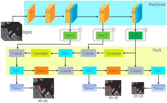
Figure 1.
Schematic of the proposed model architecture.
2.2. Efficient Backbone Network Design
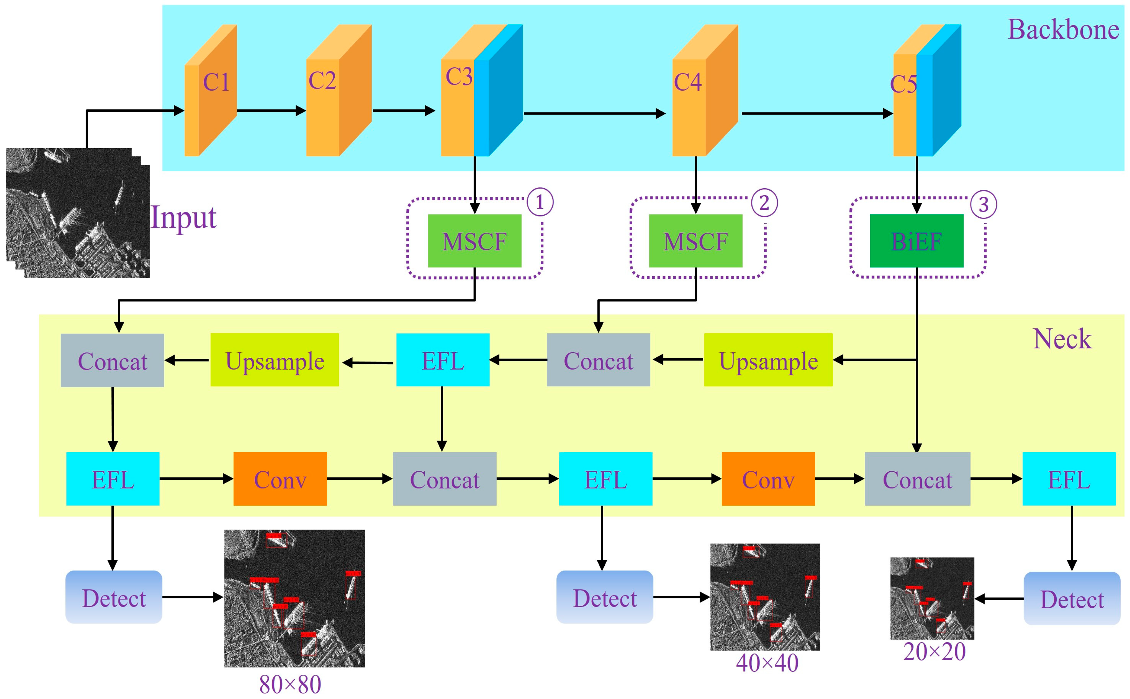
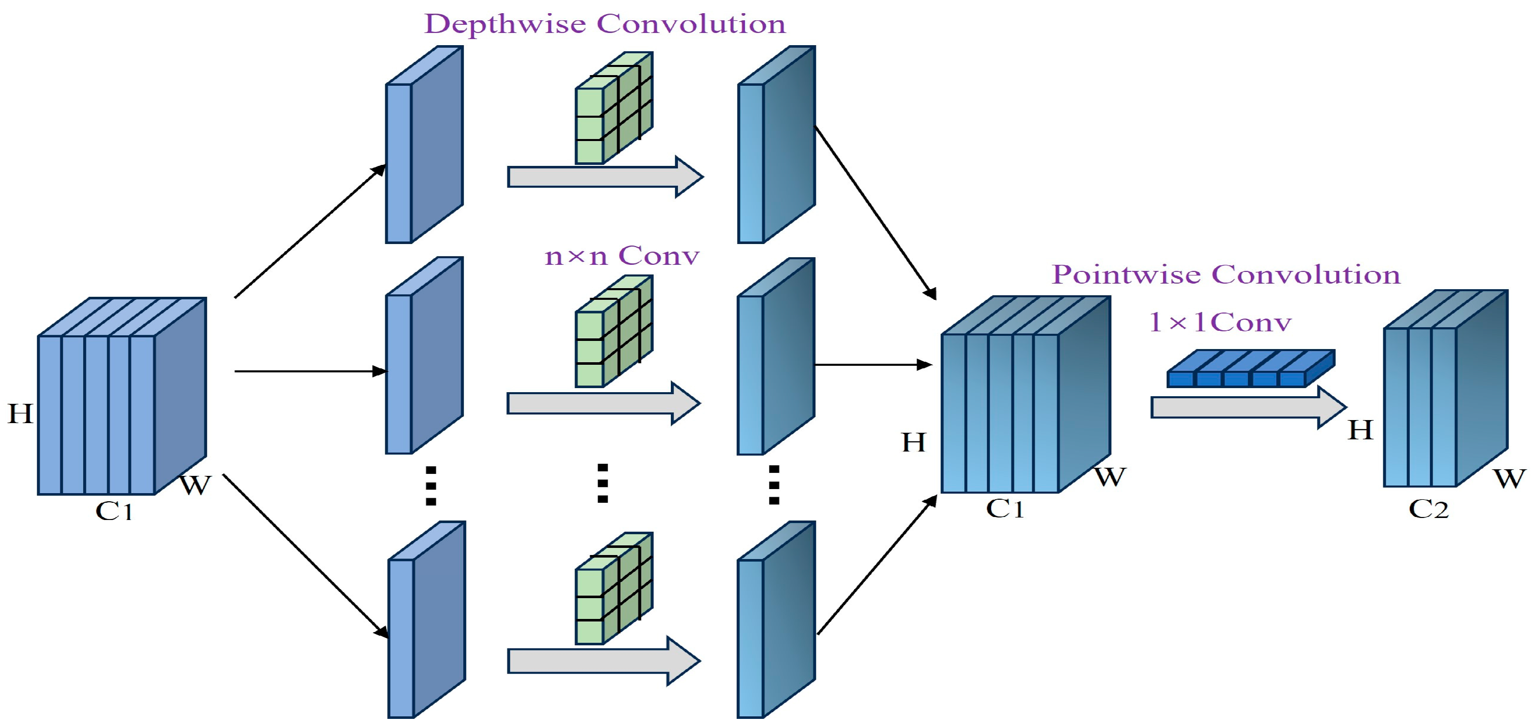
To reduce computational cost and construct a lightweight feature extraction framework, this study adopted depthwise separable convolution (DSC) as shown in Figure 2 as the core component in the backbone network. Each DSC module comprises a depthwise convolution followed by a pointwise convolution. The depthwise convolution applies a 3 × 3 kernel independently to each input channel, preserving spatial information while avoiding inter-channel interference. The subsequent 1 × 1 pointwise convolution combines outputs across channels to produce the final feature map. For example, in this work, a DSC block processes inputs from 40 to 80 channels using a 3 × 3 depthwise convolution (stride = 1 or 2, padding = 1) and then applies a 1 × 1 pointwise convolution [33]. Each convolutional operation is followed by batch normalization and an SiLU activation function to maintain numerical stability and enhance feature representation. Compared with standard convolution, which integrates spatial and channel operations simultaneously, this decoupled structure reduces computational overhead, particularly for high-resolution inputs or deeper layers.
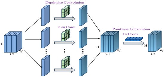
Figure 2.
Depthwise separable convolution block.
To maintain a balance between feature extraction and computational efficiency, the stage-wise allocation of DSC blocks was redesigned. Rather than directly modifying existing architectures, this study adjusted the depth of each stage based on lightweight design principles while keeping overall parameter constraints. Since excessive depth in earlier stages may introduce redundancy and insufficient depth in later stages may weaken semantic encoding, the design aimed to improve efficiency through structural optimization rather than increased depth. The stage-wise depth distribution was inspired by lightweight backbones such as ShuffleNet and MobileNet. Detailed comparative experiments are presented in Section 3.4.1 to demonstrate the effectiveness of this configuration in enhancing the extraction of informative features. Inspired by MobileNetV3, it is an effective practice to embed the attention mechanism in the deep separable convolutional block [34].
In order to avoid increasing unnecessary consumption, we have abandoned the backward residual module. In the experiment, we found that the application of CBAM [35] in the C3 and C5 layers can effectively improve the accuracy of the model, and the amount of calculation and the number of parameters increased very little. As shown in Figure 3, the CBAM module processes the input feature map and deduces the one-dimensional channel attention diagram and the two-dimensional space attention diagram in turn [36]. The overall output characteristics are calculated as follows:
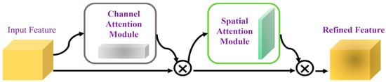
Figure 3.
Convolutional block attention module.
The operation represents element-wise multiplication, where is the feature map processed by CBAM, and and represent the channel attention and spatial attention maps, respectively.
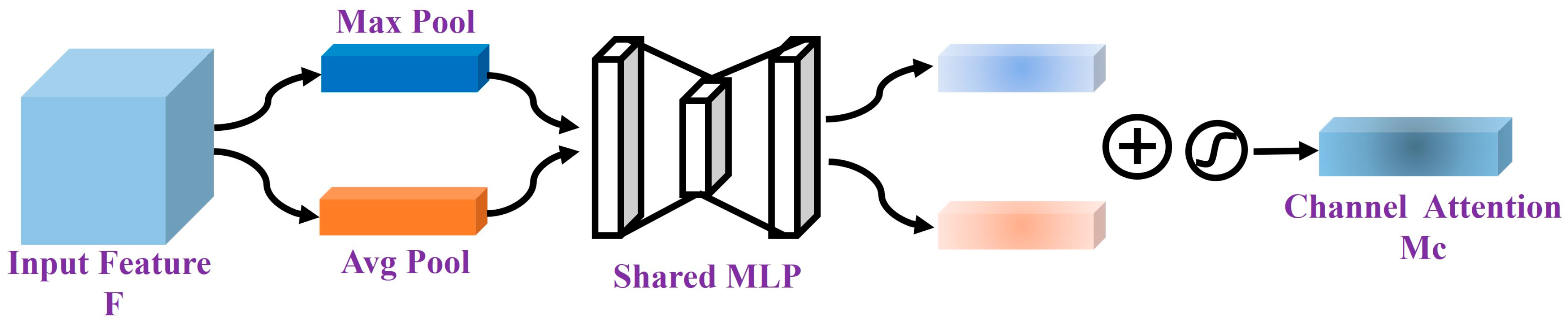
The channel attention mechanism generates two feature maps by applying global average pooling and global max pooling. These two feature maps are then passed through two layers of an MLP, where they undergo nonlinear transformations to produce the channel attention map . The detailed formula is as follows:
The function is a sigmoid function, and MLP refers to a multi-layer perceptron with weights and . represents the average pooling operation, while represents the maximum pooling operation. , where represents the height, and represents the number of channels.
The schematic diagram of the Channel attention module is shown in Figure 4.
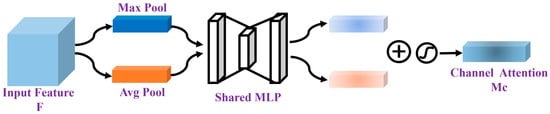
Figure 4.
Channel attention module.
The output of the spatial attention module is processed through global max pooling and global average pooling operations, resulting in two feature maps of size . These two feature maps are then concatenated and passed through a convolution (experiments show that is more effective than ) to generate a single-channel feature map [37]. After applying the sigmoid activation function, the spatial attention feature map is obtained. Finally, the output feature map is element-wise-multiplied with the original input, restoring the dimensions to . The formula for SA is as follows:
denotes the sigmoid activation function, and refers to a convolution operation with a filter size of .
The schematic diagram of the spatial attention module is shown in Figure 5.
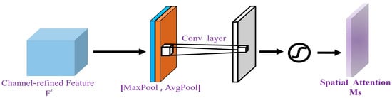
Figure 5.
Spatial attention module.
2.3. Overview of Foundational Components
To strengthen the extraction of spatial dependencies under limited computational budgets, the Efficient Multi-Scale Attention (EMA) module employs low-cost operations to enhance feature representation at both local and global scales [38]. As shown in Figure 6, the input feature map is divided into groups along the channel dimension (e.g., 32 groups), reducing computation while preserving feature diversity. Each group undergoes two directional pooling paths: height-wise pooling along columns and width-wise pooling along rows after permutation. The pooled features are concatenated and passed through a 1 × 1 convolution and then split into two branches representing height and width attention maps, which are activated by sigmoid functions and applied to the original features. Group normalization is applied to stabilize activation distributions. The normalized features are then processed by a 3 × 3 convolution to incorporate local spatial information, while a separate copy is retained as a context branch. To model inter-branch dependencies, global contextual information is extracted by applying 2D global average pooling to both branches:
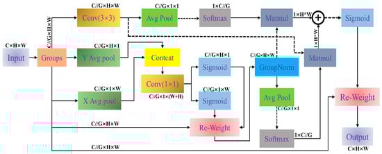
Figure 6.
Efficient Multi-Scale Attention (EMA) module. The dashed part indicates performing a “.reshape()” operation.
The pooled features are reshaped and passed through a softmax operation to generate channel-wise attention maps. These maps modulate the opposite branch via matrix multiplication: The softmax-normalized global feature of one branch weights the spatial features of the other. The resulting features are summed and passed through a sigmoid function to form a spatial attention map, which is applied to the original grouped input. Finally, the output is reshaped to the original dimensions.
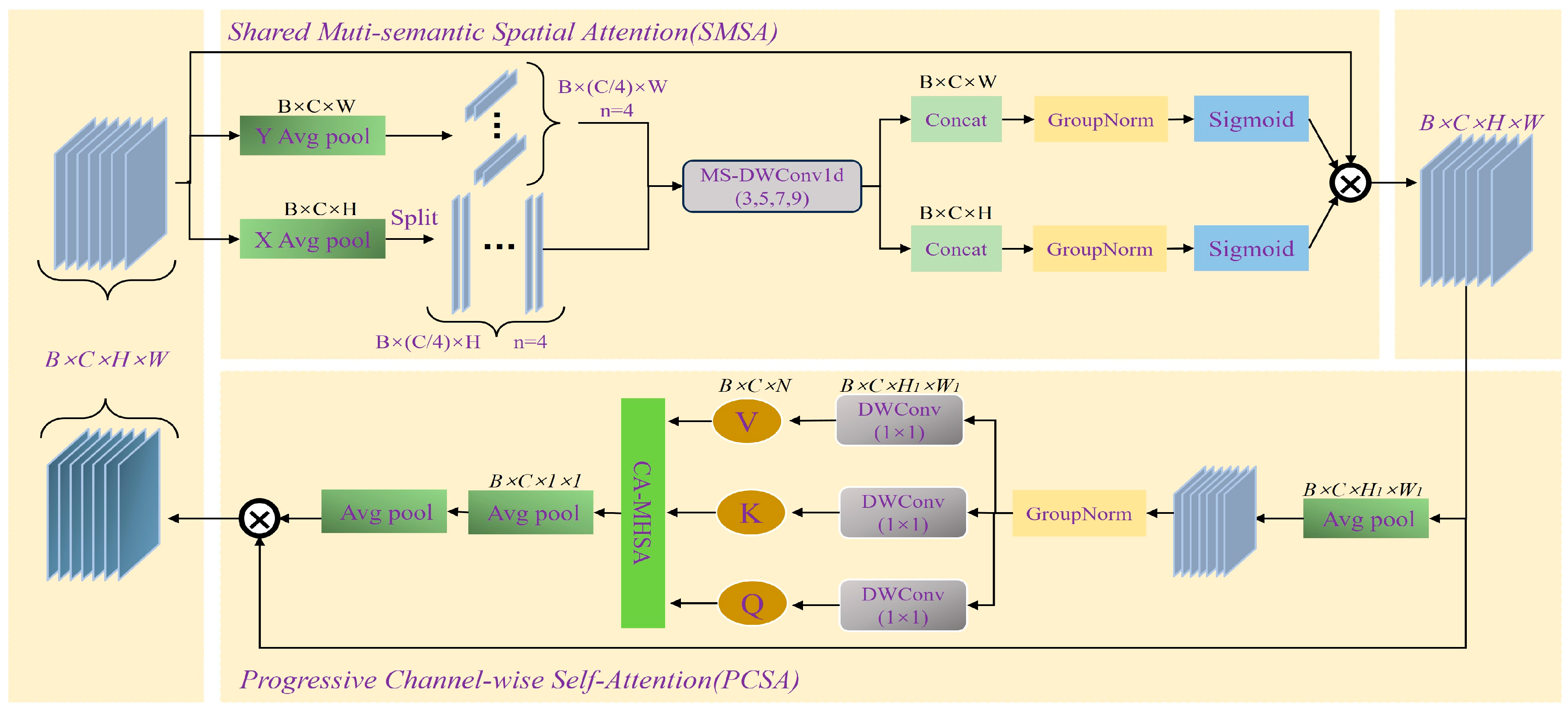
In the Shared Multi-Semantic Space Attention (SMSA) structure, the input features are first averaged and pooled along the height and width. Then, the features of and are, respectively, divided into four groups for convolution operations and concatenated together. After passing through group normalization (GN), and are obtained [39]. Finally, the two are fused onto the original input. The process in SMSA can be represented by the following formula:
represents sigmoid normalization. denotes group normalization in the H dimension with K groups. denotes the group normalization in the W dimension with K groups.
In the Progressive Channel-Wise Self-Attention (PCSA) structure, the feature input from SCSA is subjected to down-sampling operations and group normalization (GN). Then, a 1 × 1 convolution is first applied to generate more compact and representative channel features. Subsequently, the down-sampled features are decomposed into query (Q), key (K), and value (V) through a single-head self-attention mechanism [39]. Finally, the weights of the channels are further adjusted through the self-attention mechanism. The process in PCSA can be represented by the following formula:
Figure 7 provides a detailed overview of the structural layout of the SCSA module. Among them, the SMSA structure precisely extracts multi-semantic spatial information from various features, providing a solid spatial prior basis for subsequent processing. Subsequently, the PCSA module uses the overall feature mapping to perform in-depth semantic refinement on local sub-features, effectively alleviating the semantic difference problems caused by multi-scale convolutions [39]. The two complement each other and jointly improve the model’s understanding and expression abilities in complex scenarios.
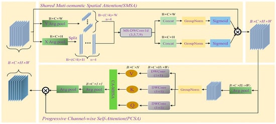
Figure 7.
Synergistic Effects Between Spatial and Channel Attention (SCSA) module.
The Efficient Fusion Learning (EFL), as shown in Figure 8, is designed to retain informative features while compressing the number of channels. The input is first processed by a 1 × 1 convolution to reduce the channel’s dimension, thereby decreasing computational cost without affecting the spatial resolution of the feature maps. A 3 × 3 convolution is then used to perform spatial feature enhancement and local fusion [32]. To balance representational capacity and model complexity, larger kernels such as 5 × 5 or 7 × 7 were not used. After batch normalization, an Efficient Channel Attention (ECA) module is applied to refine the feature representations. Specifically, ECA performs global average pooling (GAP) to summarize channel-wise statistics, followed by a 1D convolution and sigmoid activation to compute attention weights. These weights are used to reweight the input features, allowing the model to focus more on channels that are critical for target detection. This operation order is consistent with both our implementation and the illustrated structure in Figure 8.
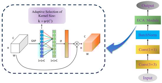
Figure 8.
Efficient Feature Learning (EFL) module.
2.4. Cross-Layer Feature Fusion and Enhancement
2.4.1. Multi-Scale Coordinated Fusion (MSCF) Module
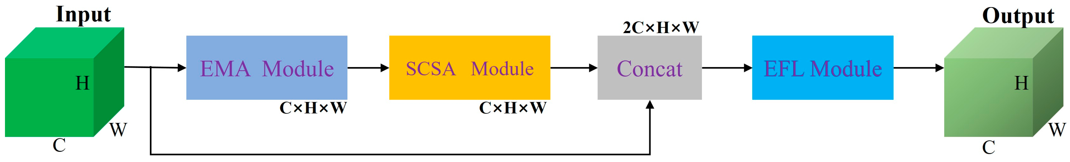
To address the challenges of multi-scale targets and complex background interference in SAR ship detection, we propose the Multi-Scale Coordinated Fusion (MSCF) module, as illustrated in Figure 9. MSCF integrates the EMA, SCSA, and EFL modules in a coordinated manner, with each component focusing on a specific aspect of representation enhancement—global context aggregation, multi-scale semantic extraction, and channel-wise refinement. Specifically, the EMA module performs feature smoothing and compression through global average pooling, which emphasizes global information and reduces noise from complex backgrounds or low signal-to-noise ratio environments. The SCSA module applies convolutional kernels of sizes 3 × 3, 5 × 5, 7 × 7, and 9 × 9 to extract multi-scale contextual information, while the EFL module employs compact convolutions and attention-based weighting to refine features efficiently, avoiding unnecessary computational burden.

Figure 9.
Multi-Scale Coordinated Fusion (MSCF) module.
This module is deployed at the shallow-to-intermediate stages of the backbone (see Figure 1), where feature maps maintain relatively high spatial resolution. Placing MSCF at these stages allows the early improvement of spatial and semantic representations, supporting the detection of small targets and the suppression of background interference. The combination of these modules enables MSCF to effectively integrate spatial-, scale-, and channel-level cues. Its performance and complementarity with the BiEF module will be further validated through the ablation studies in Section 3.4.3.
2.4.2. Bi-EMA Enhanced Fusion (BiEF) Module
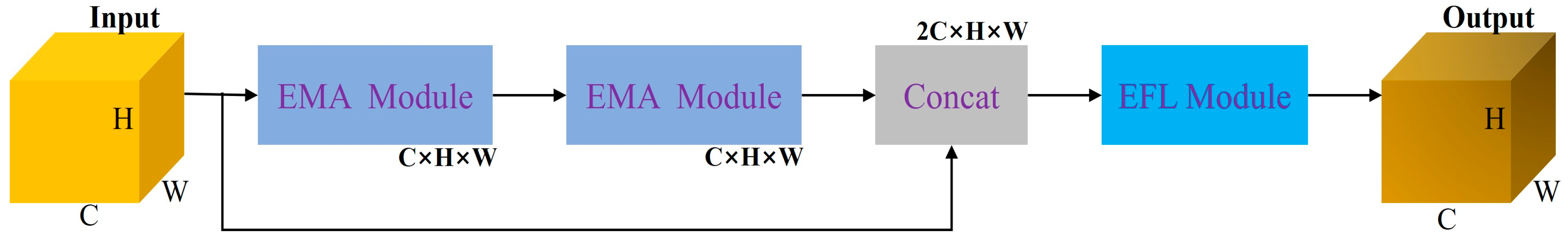
In the deepest backbone layer—reduced to a spatial resolution of 20 × 20 due to five down-sampling operations—large convolution kernels such as 7 × 7 or 9 × 9 are less effective for capturing broader context. Therefore, SCSA is not adopted in the deepest layer. To enhance multi-scale semantic representation at this stage, a Bi-EMA Enhanced Fusion (BiEF) module is adopted, as illustrated in Figure 10. Unlike MSCF, BiEF omits the SCSA component and instead applies the EMA module twice in succession, followed by the EFL module.

Figure 10.
Bi-EMA Enhanced Fusion (BiEF) module.
The dual-EMA design is inspired by double-attention architectures such as A2-Nets [40] (“Double Attention Networks”), where two attention steps sequentially gather and distribute global context, improving deep-layer feature refinement. Accordingly, the two EMA passes in BiEF aim to reduce redundancy and reinforce fine-grained semantic details within a compact spatial domain. The resulting features are concatenated with the original input and processed via EFL to complete channel-wise fusion.
Since the structures of EMA and EFL are detailed in Section 2.3, they are not repeated here. The distinctive role of BiEF in deep-layer integration and its complementarity with MSCF will be further evaluated through ablation studies in Section 3.4.3.
2.5. EFL-Based Efficiency Boost
In the neck structure of the network, the Feature Pyramid Network (FPN) and Path Aggregation Network (PAN) are employed to enhance multi-scale feature integration. FPN transmits semantic information from deeper layers to shallower ones, while PAN strengthens the bottom–up path, enabling the preservation of fine-grained spatial details. However, the original C2f modules embedded in these layers introduce notable redundancy due to their hierarchical residual design and repeated convolutional operations, which may affect efficiency under limited computational resources. To address this issue, the C2f modules are replaced by the Efficient Feature Learning (EFL) module, which performs a similar dimensional transformation while simplifying the internal structure. As described in Section 2.3, EFL utilizes 1 × 1 convolutions for channel adjustment and 3 × 3 convolutions for local feature enhancement. This configuration reduces both parameters and computational cost while preserving spatial resolution. The embedded channel attention mechanism helps the model emphasize informative channels, which is beneficial for detecting small or low-contrast targets in complex backgrounds. The integration of EFL into the FPN + PAN framework supports a more lightweight and effective fusion process across different semantic levels.
Given that its structure has been detailed in Section 2.3, this section focuses on its application strategy within the neck network. By replacing C2f with EFL, the model maintains adequate feature interaction. A comparative ablation analysis involving C2f, ECA [32], and the Efficient Feature Learning (EFL) module is presented in Section 3.4.4 to validate the replacement strategy and examine its effectiveness in enhancing detection performance [41].
3. Results
3.1. Dataset
In this experiment, we selected the SAR Ship Detection Dataset (SSDD), the first open-source dataset in the field of SAR ship detection, which holds considerable research value.
Regarding data collection, the dataset includes scenes from nearshore and offshore regions, such as Yantai, China, and Visakhapatnam, India, offering a realistic representation of the complex and varied monitoring environments and making the model training more applicable to real-world scenarios [19]. SSDD integrates images from various sensors, including RadarSat-2, Terra SAR-X, and Sentinel-1, with resolutions ranging from 1 m to 15 m. The dataset includes multiple polarization modes, such as HH, VV, VH, and HV.
As shown in Figure 11, we selected a subset of images from the SSDD dataset for visual analysis of the experimental results.
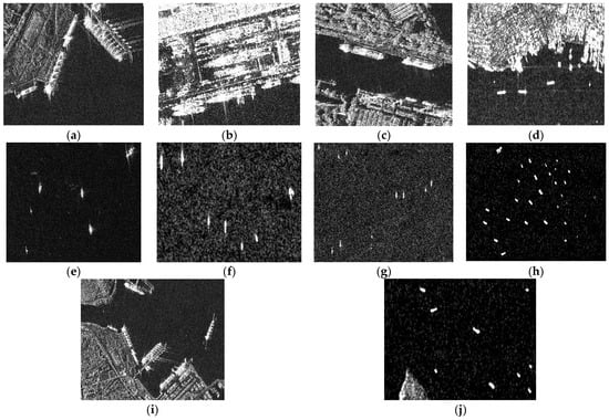
Figure 11.
Examples from the SSDD dataset. (a–d,i) Examples of inshore ships. (e–h,j) Examples of offshore ships.
3.2. Experimental Environment and Details
In this study, all experiments were conducted on a Windows 11 operating system, with the computing platform built around an AMD Ryzen 7 7840H processor and an NVIDIA GeForce RTX 4060 graphics card operating at a base frequency of 3.8 GHz and equipped with 16 GB of memory. The development environment included Python 3.9.19 and Torch 2.4.1, with GPU acceleration provided by CUDA 11.8.
During testing, the Adam optimizer was employed with a batch size of 16 and 300 epochs. The initial learning rate was set to 0.001 and was reduced using a cosine annealing schedule to minimize the loss function.
To ensure fairness and consistency in the comparative analysis, all experimental results reported in this paper were obtained under the unified experimental conditions described in this section. These conditions include consistent training settings, dataset partitioning, and evaluation metrics across all models.
3.3. Evaluation Criteria
To accurately evaluate the performance of each component in the experiment, we employ four key metrics: recall, precision, mAP50, and F1 score.
Recall measures the model’s ability to detect all the actual targets present, while precision evaluates the proportion of true positive samples among all samples predicted as targets. The F1 score is the harmonic mean of precision and recall. The formulas for each metric are as follows:
TP: True positives refer to the targets that the model correctly detects. FN: False negatives are the actual targets that the model fails to detect. FP: False positives are non-targets that the model incorrectly identifies as targets [42].
mAP: The mean average precision is used to evaluate the average accuracy of detection boxes across different categories, with an IoU threshold of 0.5.
3.4. Ablation Experiment
To comprehensively validate the effectiveness of the proposed method, four ablation experiments were carefully designed. In each experiment, the principle of single-variable control was strictly followed, and targeted adjustments to different application methods were carried out to systematically analyze their impact on model performance.
3.4.1. The Impact of Different Depths on the Backbone Network
This section investigates the impact of different backbone depths on model performance. The backbone consists of five layers, with the depth of the first layer fixed at 1. The depths of the remaining four layers are varied for comparison across the following configurations: [1,2,2,1], [2,2,2,2], [2,3,3,2], [3,3,3,2], [3,3,3,3], [3,4,4,3], and [4,4,4,4]. Table 1 presents the precision (P), recall (R), mean average precision (mAP), and F1 score of each configuration. The model performed optimally when the backbone depth was set to [3,3,3,2], achieving the highest values for all evaluation metrics.

Table 1.
Ablation experiment for backbone depth.
The selection of these configurations was driven by the design of the backbone network (Section 2.2), which aimed to optimize performance. The configuration [3,3,3,2] achieved the highest performance across multiple metrics, indicating its effectiveness in feature extraction. Variations from this optimal configuration resulted in a decrease in performance, suggesting that changes in depth reduced the model’s ability to effectively extract features. These findings guided the choice of depthwise separable convolution blocks in the backbone network, which were selected based on the best-performing configuration: [3,3,3,2].
3.4.2. Comparison of Different Attention Mechanisms in Backbone Networks
This section investigates the performance of various attention mechanisms integrated with a feature extraction network composed of depthwise separable convolution blocks, as described in Section 2.2. The evaluated attention modules include ECA [32], SE [43], CA [44], PSA [45], and CBAM. The comparison results are presented in Table 2.
Table 2.
Comparison experiment of different attention mechanisms in backbone network.
Among all variants, the model incorporating CBAM achieved the highest precision, recall, mAP, and F1 score. The SE module attained a similar mAP, with only a 0.05% difference, but it showed a 3.15% lower recall. The ECA module had a 0.25% lower mAP than CBAM, with a precision gap of 0.92% and a recall gap of 5.72%. CA and PSA resulted in more noticeable decreases across all metrics. These results indicate that CBAM was more effective in enhancing the representation capability of the backbone network when combined with depthwise separable convolution blocks.
3.4.3. Experiment of Fusion Module at Different Backbone Output Points
To examine the role of the proposed fusion modules (MSCF and BiEF), ablation experiments were conducted at three predefined positions, as illustrated in Figure 1. The baseline (Number 1), with all fusion modules disabled, achieved a precision of 98.99%, recall of 88.91%, mAP of 97.28%, and F1 of 0.94. As shown in Table 3, in partial configurations (Numbers 2 to 5), the results showed varying performance. For instance, enabling MSCF at Positions 1 and 2 (Number 2) led to a slight decrease in performance across all metrics. This outcome suggests that shallow fusion, when applied alone, may introduce redundant features or fail to provide sufficient semantic reinforcement. In configurations Number 3 to 5, where BiEF was placed at Position 3, either alone or with MSCF at one additional position, recall improved while precision declined, and mAP remained close to the baseline. These observations indicate that the performance of individual modules or their combination without proper structural coordination does not consistently enhance detection accuracy.
Table 3.
Ablation experiment of the fusion module at different backbone output points.
In contrast, the full configuration (Number 6), which applies MSCF at Positions 1 and 2 and BiEF at Position 3, resulted in the highest performance across all metrics. This pattern indicates that the two modules contribute differently: MSCF is more effective at capturing spatial-scale information at earlier stages, while BiEF aids in semantic refinement at deeper layers. Their combined use provides complementary effects that are not observed when the modules are used independently.
To further assess whether MSCF and BiEF modules are functionally interchangeable, two additional experiments were conducted: one applying BiEF at all three positions and another applying MSCF at all positions. The configuration using BiEF at all positions achieved a precision of 98.22%, recall of 92.67%, and mAP of 98.14%. The configuration using MSCF at all positions resulted in a precision of 98.13%, recall of 92.33%, and mAP of 98.06%. Compared to the heterogeneous combination in Number 5, both homogeneous configurations showed lower mAP and F1 scores. These results confirm that MSCF and BiEF are not fully interchangeable, and their combination offers complementary benefits.
The findings support the design choice outlined in Section 2.4, where MSCF is placed at earlier stages to capture spatial and scale information, and BiEF is utilized at the final stage to enhance deep semantic features. The heterogeneous placement consistently outperforms homogeneous alternatives. Furthermore, the ablation results suggest that performance improvements do not stem from the mere addition of fusion modules but from their complementary and coordinated integration across multiple stages, which collectively enhance feature representation and detection accuracy.
3.4.4. Comparison of ECA, EFL, and C2f Modules
The original model uses the C2f module in the neck structure, which improves the information flow and feature utilization between different layers through large residual connections. However, in SAR ship detection, the C2f module shows limited improvements in both detection accuracy and recall. To address this, we propose replacing the C2f module with the EFL module, which combines convolution operations with a channel attention mechanism to improve feature fusion. The ECA module, which employs 3 × 3 and 1 × 1 convolutions, is also included for comparison.
As shown in Table 4, the EFL module outperforms the C2f module across all evaluation metrics. Specifically, the mAP increases by 0.23%, recall improves by 0.83%, and accuracy rises by 0.45%, indicating that the EFL module is more effective in enhancing detection performance. While the ECA module also shows improvements over the C2f module, its performance is slightly lower than the EFL module, particularly in mAP.
Table 4.
Comparative analysis of C2f, ECA, and EFL modules.
These results show that the EFL module provides better improvements in recall and mAP, making it a more effective choice for SAR ship detection tasks. The ECA module is beneficial, but the EFL module offers more substantial performance gains, demonstrating its more effective role in improving model performance.
3.4.5. Overall Ablation Study
In Section 3.4.1, Section 3.4.2, Section 3.4.3 and Section 3.4.4 a series of ablation experiments were conducted using a controlled variable approach. Each experiment examined the effect of introducing a single structural module—CBAM, BiEF, MSCF, or EFL—while keeping other components unchanged. This method allowed an independent evaluation of each module under consistent experimental settings. It was observed that in some of these experiments, the introduction of a single module resulted in a slight decrease in one or more evaluation metrics. Such results suggest that individual components may not always align optimally when applied in isolation and that their integration may introduce structural redundancy or inconsistencies in feature interaction.
To further analyze the overall behavior of the proposed architecture, a comprehensive ablation experiment was conducted. Based on the DSC-Backbone, additional modules were integrated incrementally to form five variants, as listed in Table 5. Each configuration was evaluated under identical training conditions to examine the effect of progressive module fusion on detection performance. All experimental settings, including dataset, input size, training schedule, and evaluation metrics, were kept consistent across variants. This ensures comparability between different structural combinations and avoids the influence of external variables.
Table 5.
Overall ablation study with progressive integration of proposed modules.
The ablation study shown in Table 5 (steps 1–5) focuses on individual modules and their stepwise integration, which focused on individual modules and their progressive integration, a supplementary set of experiments was conducted to examine key combinations of the proposed modules. This additional experimental design aims to extend the analysis by capturing interactions between multiple modules simultaneously, offering a more nuanced understanding of their collective influence within the overall architecture. The combinations tested were DSC + MSCF + BiEF, CBAM + MSCF + BiEF, and MSCF + BiEF + EFL, along with several other relevant groupings. These experiments serve as a supplementary investigation addressing combinations of modules not covered in the previous studies. The selected configurations aim to enhance the completeness and focus of the analysis while minimizing redundancy and covering the fundamental aspects of module integration. The results, as summarized in Table 5 (Steps 7–12), provide additional information that complements the earlier findings and supports a more comprehensive evaluation of module fusion strategies.
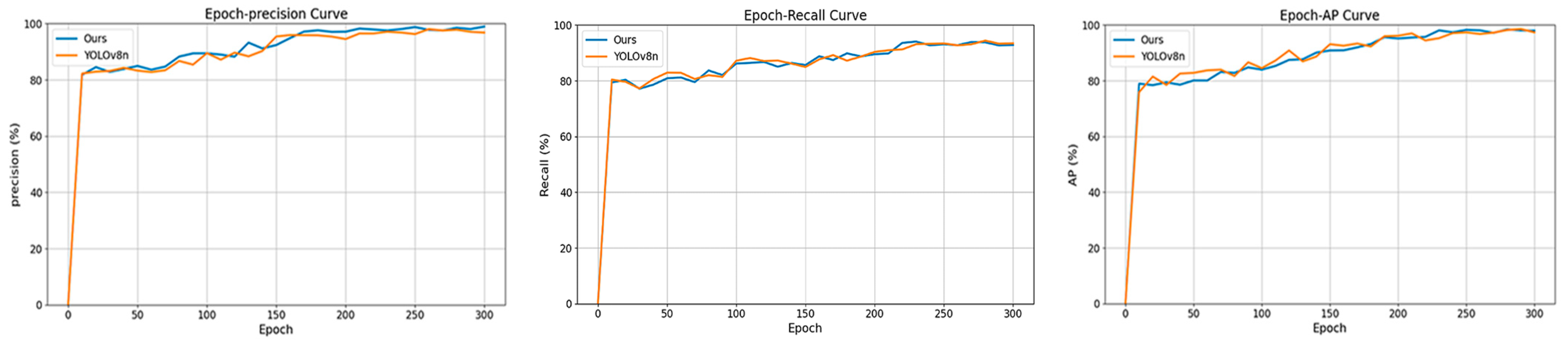
The introduction of the epoch-based precision, AP, and recall curves (Figure 12) serves to further illuminate the training dynamics and performance evolution as the modules were incrementally added. These curves offer a clear visualization of how each model variant’s performance improved over time, particularly with respect to precision, average precision (AP), and recall metrics. By tracking these metrics across different epochs, deeper insights can be gained into how the gradual integration of modules enhances the overall model’s detection capabilities and stability during training.
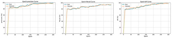
Figure 12.
Comparison of YOLOv8n and our model in terms of precision, recall rate, and AP0.5 during the training process.
3.5. Comparison with Other Ship Detection Models
Table 6 summarizes the performance of the proposed model and several representative lightweight detectors on the SSDD dataset. Among these, the proposed model achieves the highest accuracy (98.76%) and the second-highest recall (93.70%), with an mAP of 98.35% and an F1 score of 0.96. Compared to YOLOv11n and YOLOv12n, the proposed model shows slightly higher accuracy and mAP while maintaining a comparable F1 score. Specifically, YOLOv11n achieves an accuracy of 98.32%, a recall of 93.15%, and an mAP of 98.22%, while YOLOv12n yields a slightly higher recall (94.01%) but lower accuracy and mAP.
Table 6.
Performance evaluation of various mainstream models on the SSDD dataset.
From the results in Table 6, despite improvements in computational efficiency, the detection performance of PC-Net [46] and LCFANet-n [47] is generally lower than that of YOLOv8n, particularly in accuracy and mAP. This suggests that reduced computational complexity does not always correlate with enhanced detection effectiveness.
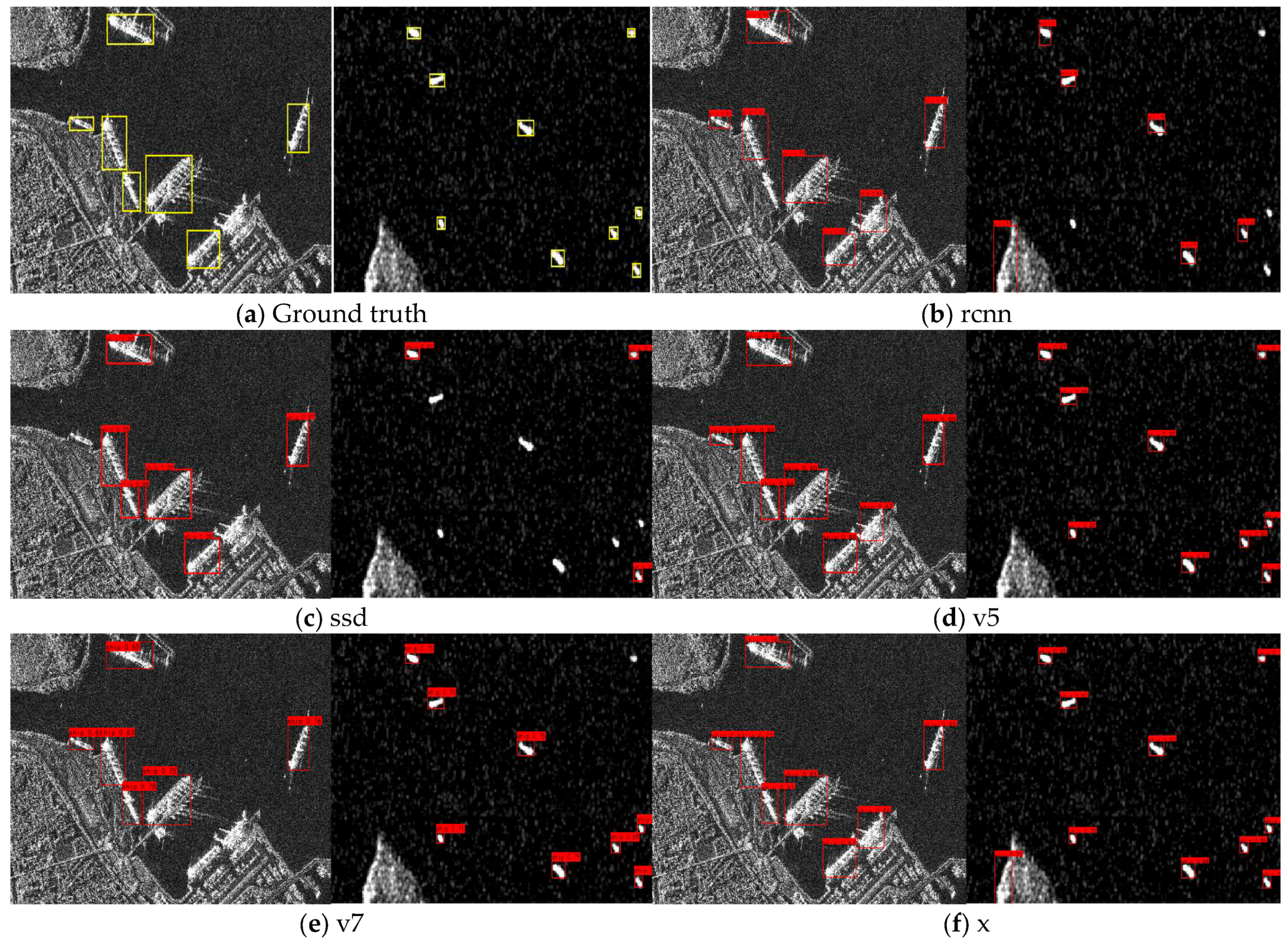
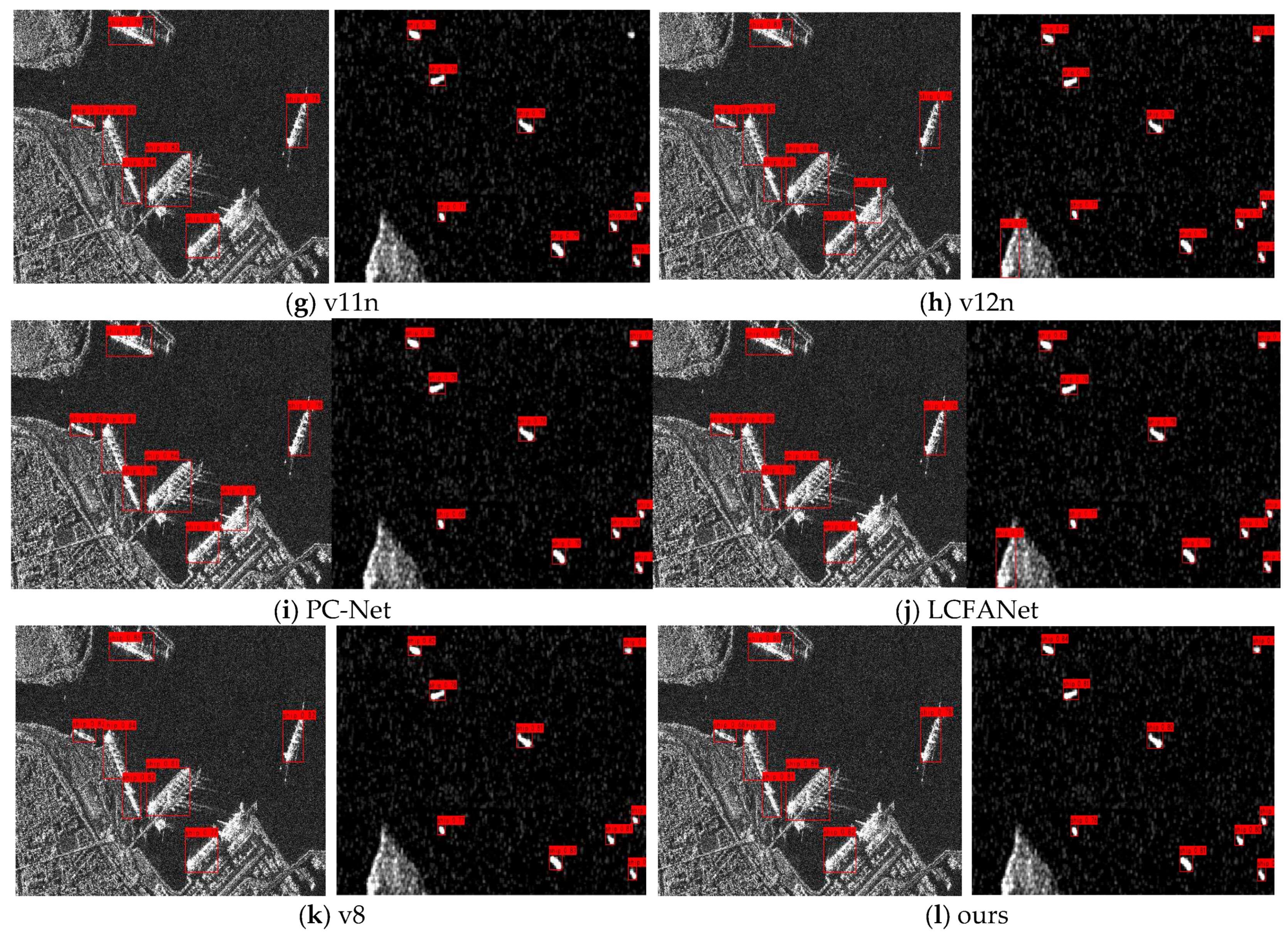
In terms of computational efficiency, the proposed model has the lowest resource demand among all compared models, with 5.04 G FLOPs and 1.64 M parameters. This is 17.8% and 29.3% lower than PC-Net and 16.4% and 36.4% lower than YOLOv12n in terms of FLOPs and parameter count, respectively. Compared to YOLOv8n, which also shows competitive performance, the proposed model reduces FLOPs and parameters by 47.5% and 48.1%, respectively. Other models such as Faster R-CNN and SSD show higher computational costs or reduced detection capability. For instance, Faster R-CNN has high recall but low accuracy and very large computational demands (370.21 G FLOPs and 139.10 M parameters), making it unsuitable for real-time deployment on resource-constrained platforms. SSD has moderate computational complexity but suffers from low recall, which limits detection coverage. Considering both detection performance and computational cost, the proposed model achieves a favorable balance. Its high accuracy and recall ensure reliable detection, while the low FLOPs and parameter count support deployment in constrained environments such as satellites. This balance enables the precise identification of maritime targets while adhering to the stringent computational, storage, and power constraints imposed by satellite onboard systems. Among the evaluated models (as shown in Figure 13), only our model and YOLOv8n successfully detected all targets. The proposed model achieves marginally higher accuracy (98.76% compared to 97.15%) and exhibits higher confidence scores among the correctly detected targets. Compared to the latest PC-Net and LCFANet-n, the proposed model achieves higher detection accuracy along with reduced computational complexity and fewer parameters, reflecting an improved balance between performance and efficiency.
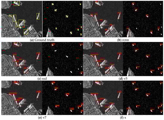
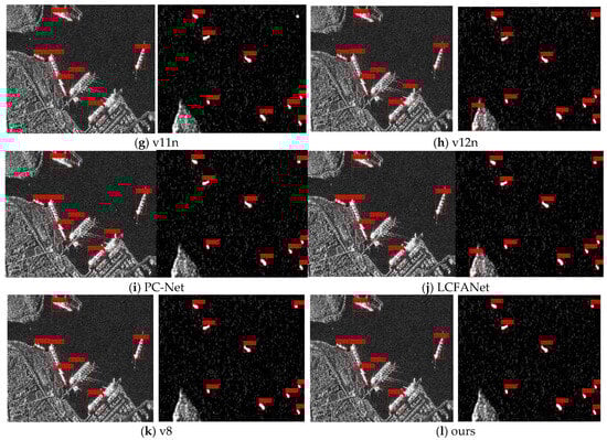
Figure 13.
Comparison of target detection results on the SSDD dataset. (a) Ground truth. (b) Visualization of Faster R-CNN detection results. (c) Visualization of SSD detection results. (d) Visualization of YOLOv5s detection results. (e) Visualization of YOLOv7-tiny detection results. (f) Visualization of YOLOX-tiny detection results. (g) Visualization of YOLOv11n detection results. (h) Visualization of YOLOv12n detection results. (i) Visualization of PC-Net detection results. (j) Visualization of LCFANet-n detection results. (k) Visualization of YOLOv8n detection results. (l) Visualization of our detection results.
3.6. More Visual Detection Results
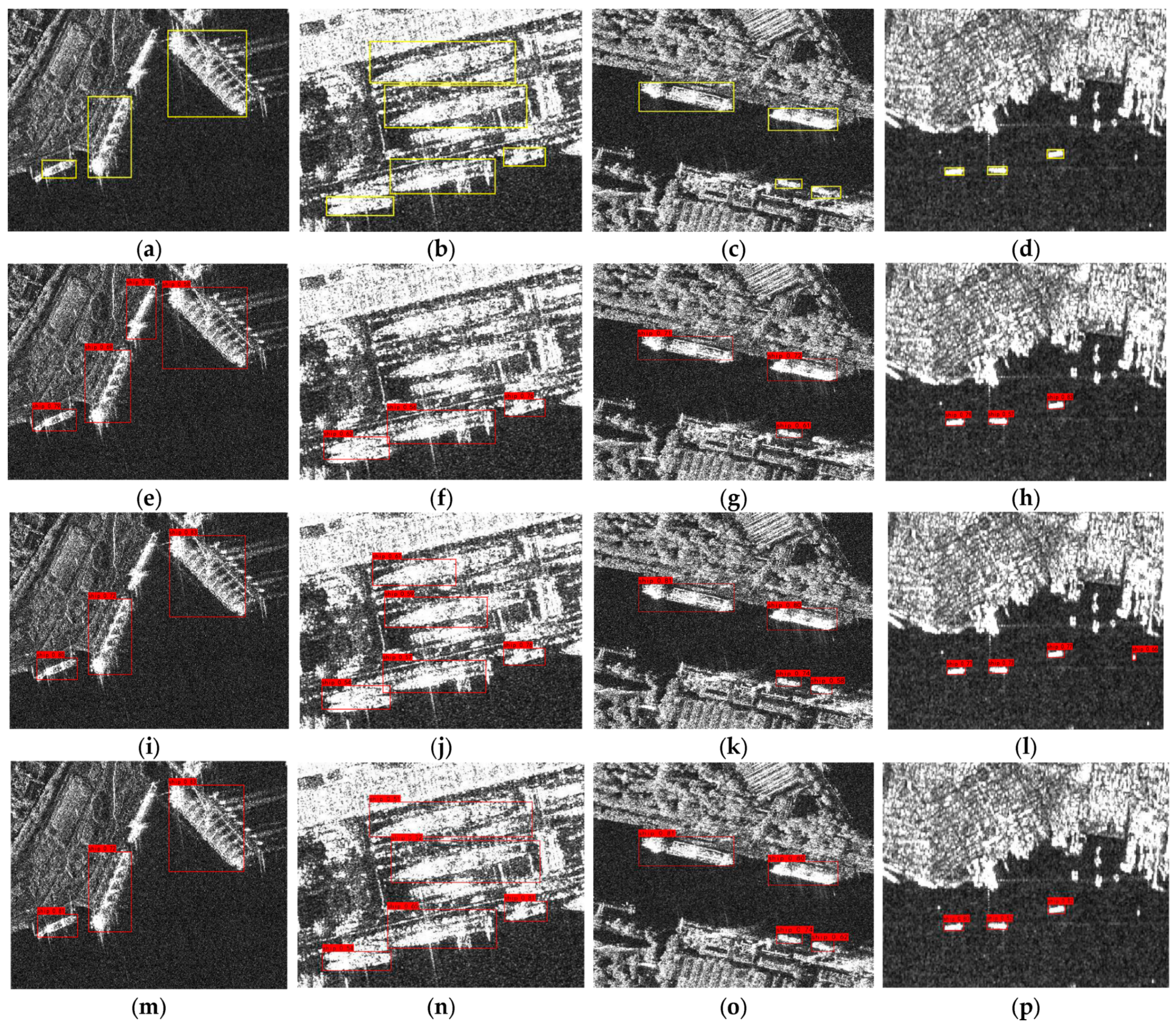
More inshore and offshore scenarios were detected using our LCFANet model and YOLOv8n, with the results are presented in Figure 14 and Figure 15. In these figures, the true targets are highlighted with yellow bounding boxes in the ground truth for comparison.
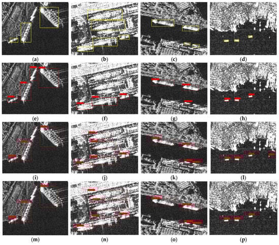
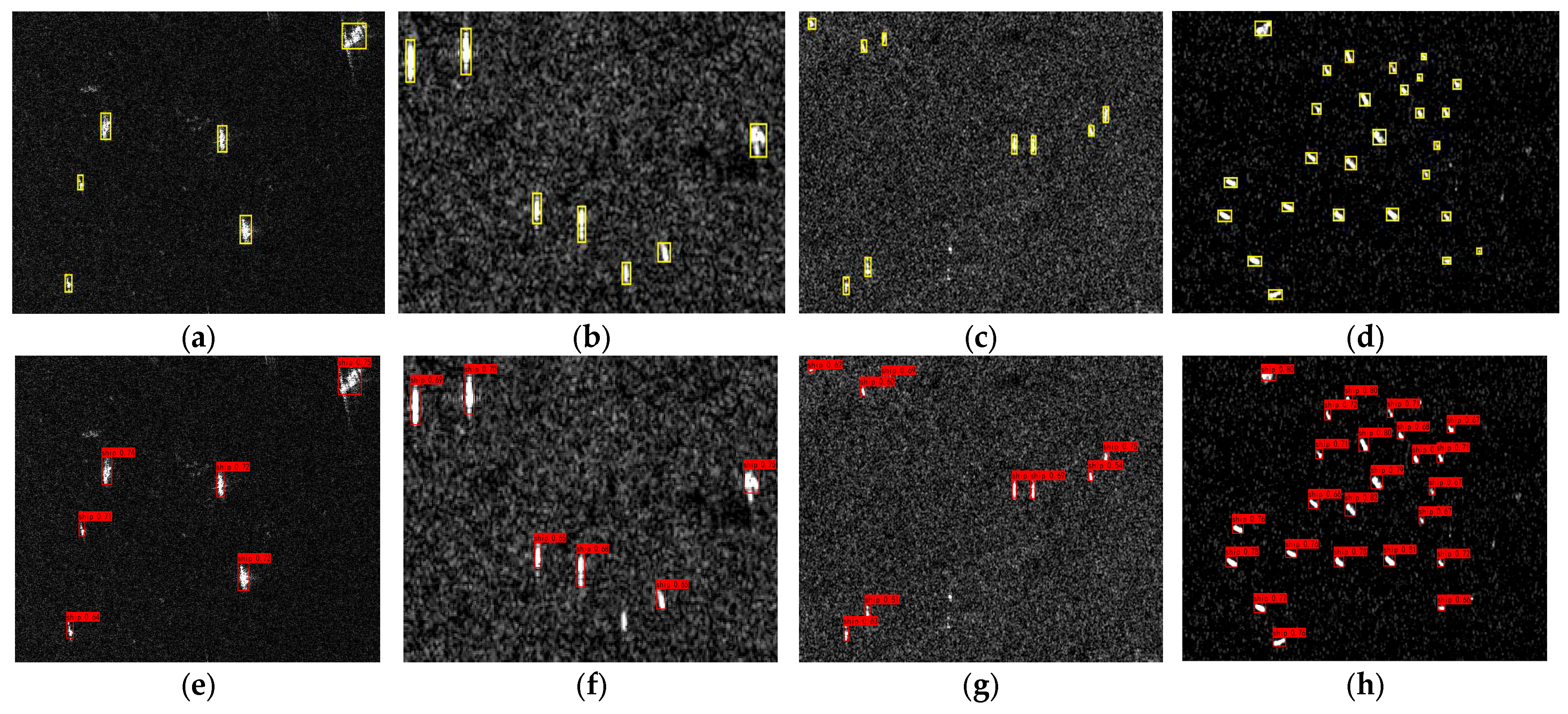
Figure 14.
Detection diagram of the inshore scene. (a–d) Ground truth, (e–h) LCFANet-n, (i–l) YOLOv8n, and (m–p) our model.

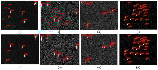
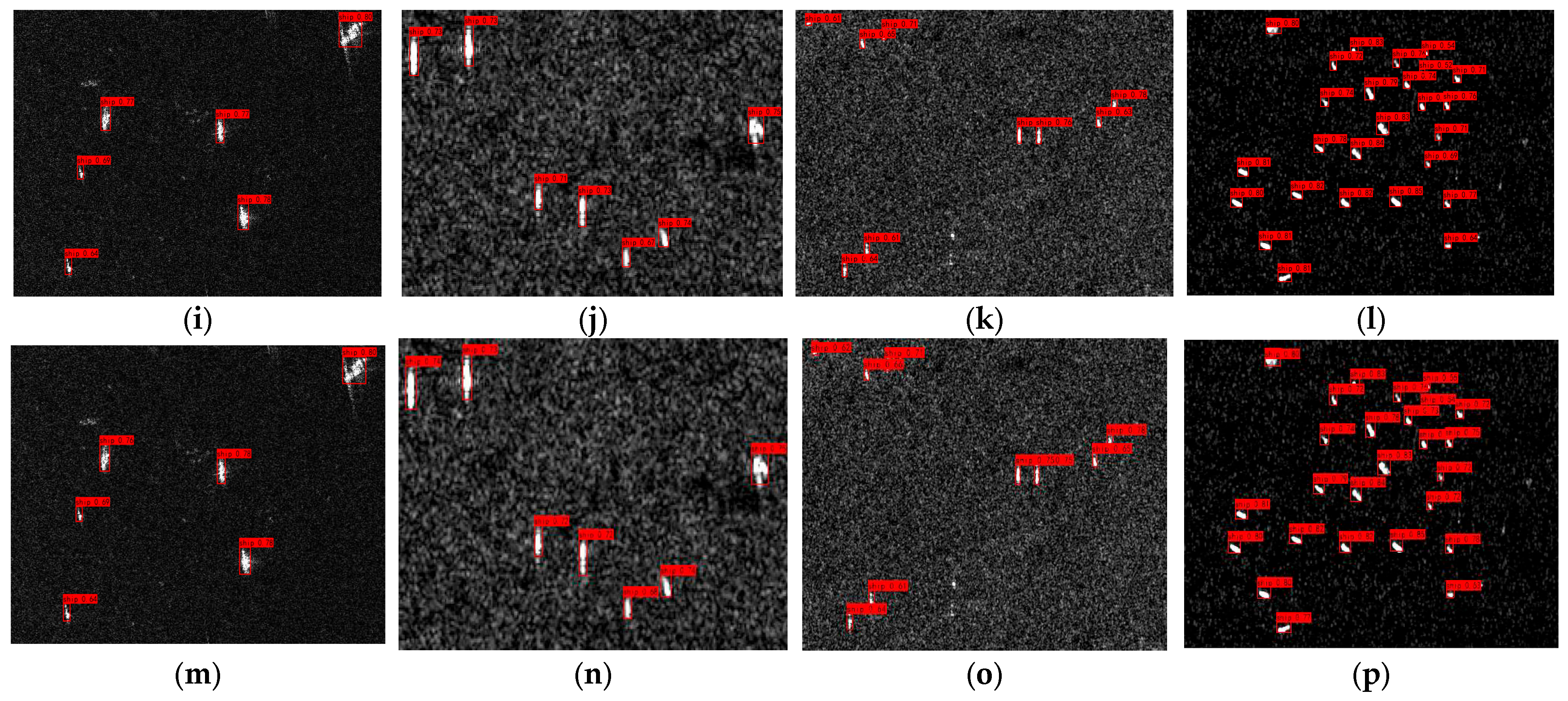
Figure 15.
Detection diagram of the offshore scene. (a–d) Ground truth, (e–h) LCFANet-n, (i–l) YOLOv8n, and (m–p) our model.
These images were selected from a subset of the SAR Ship Detection Dataset (SSDD), which contains real-world data with varying noise levels that naturally occur in maritime environments. The data in the SSDD dataset are derived from operational SAR systems and represent a wide range of imaging conditions, including different sea states and sensor configurations. For the analysis in this study, the signal-to-noise ratio (SNR) was computed for each target in the selected images based on the power of the signal and the power of the background noise. The signal power was calculated as the sum of the squared pixel values within the target region, while the background noise power was estimated using the variance of the pixel values in a surrounding background region, which was assumed to contain no targets. The SNR for each target in the image was calculated using the following formula:
where is the signal power (sum of the squared pixel values in the target region), and is the noise power (variance of the pixel values in the background region). This approach provides a clear measure of how the model performs in various noise conditions that are typical in SAR imagery [48]. Additionally, for each image, the average SNR across all targets was computed to provide an overall understanding of the image’s noise characteristics. The average SNR was calculated using the following formula:
where n is the number of targets in the image, and is the SNR for each individual target. This average SNR provides a comprehensive measure of the image’s overall noise level.
The images selected for this section exhibit inherent variations in the signal-to-noise ratio (SNR), with values spanning from 10 dB to 22 dB. These differences reflect the natural diversity found within the SSDD dataset [19], which contains a variety of imaging conditions influenced by factors such as sensor type, resolution, and environmental settings. Figure 14 and Figure 15 present examples of these variations, where some images exhibit higher background noise while others show lower noise levels, illustrating the dataset’s broad range of noise characteristics.
3.7. Theoretical Analysis of Computational Complexity
To quantitatively evaluate the computational cost of the proposed model, we conduct a theoretical analysis based on two commonly used metrics: the number of parameters (Params), which reflects the storage requirements, and floating-point operations (FLOPs), which estimate the computational complexity during inference. In convolutional neural networks, the primary computational load arises from convolutional layers. The number of parameters and FLOPs for a standard convolution layer are calculated as follows:
where Cin and Cout represent the number of input and output channels, K is the kernel size, and H × W is the resolution of the output feature map. The multiplier of 2 accounts for both multiplication and addition operations, following conventions adopted in YOLO and related works.
While convolutional layers dominate the computational cost, other operations also contribute to the overall complexity. For example, attention modules such as CBAM and ECA introduce additional convolution, pooling, and activation operations. The fully connected layers used in some modules add matrix multiplications and bias terms. Pooling, interpolation, and concatenation operations, though parameter-free, also involve memory and arithmetic operations. Therefore, convolution-based formulas serve as the foundation for complexity estimation, supplemented by empirical analysis using the thop profiling tool.
Under an input resolution of 640 × 640, we evaluated the computational complexity of each component of our network. The results are listed in Table 7:
Table 7.
The parameters and computational complexity of each part of the proposed model.
Compared to the YOLOv8n model, which contains 3.16 million parameters and 8.86 GFLOPs, the proposed model shows a 48.1% reduction in parameters and a 47.5% reduction in FLOPs. These reductions are associated with the application of lightweight components such as depthwise separable convolutions and simplified attention mechanisms.
4. Discussion
A detailed analysis of the experimental results illustrates the structural characteristics of the proposed model and offers insights for future refinement. In the ablation experiments on the backbone network, the optimal configuration for the depthwise separable convolution blocks was identified as [3,3,3,2], which offers a rational setup for the backbone network. This convolutional strategy, based on depthwise decomposition, reduces computational cost while preserving accuracy, supporting the lightweight objective. In the comparison of different attention mechanisms, CBAM yielded the best overall performance with limited additional computational overhead. Compared to the SE module, while precision remained similar, CBAM improved the recall rate by 3.15%, suggesting enhanced capability in reducing false negatives and capturing more informative features within the backbone. The BiEF and MSCF modules, through cross-layer feature interaction, build a joint spatial-channel perception framework. The fusion module position experiments showed that the combination of both modules effectively integrates multi-level features from the backbone network while retaining fine-grained features, addressing challenges associated with targets of various sizes and complex backgrounds. This resulted in an mAP of 98.35%. The EFL module optimized the feature fusion process, leading to improvements after replacing the C2f module: mAP increased by 0.89%, F1 score rose by 0.03, recall improved by approximately 4.39%, and precision increased by 1.34%.
When compared with existing models, the proposed approach exhibits strong performance in terms of precision (98.76%), mAP (98.35%), and F1 score (0.96) while also offering significant advantages in computational complexity and parameter size. Its lightweight design is particularly important for resource-constrained satellite devices, enabling real-time detection under limited computational resources.
5. Conclusions
This study proposes a lightweight model for SAR ship detection tasks on satellite platforms and evaluates its performance through comprehensive experiments. With the customized backbone network and novel efficient feature fusion modules, the model achieves effective feature extraction and inter-level information interaction. The experimental results show that the model achieves detection accuracy comparable to YOLOv8n on the SSDD dataset, while its parameter size is only 1.64 M and its computational complexity is 5.04 G, which are reduced by 48.1% and 47.5%, respectively, compared to YOLOv8n. These results indicate the model’s strong suitability for resource-constrained environments.
This research provides a new technical pathway for real-time SAR ship detection on satellite platforms. Future work could focus on further exploring the optimization of module combinations to fully exploit the model’s potential, thereby enhancing detection accuracy and robustness to better meet the diverse and dynamic demands of practical applications.
Author Contributions
Conceptualization, W.X.; methodology, W.X. and Z.G. (Zengyuan Guo); software, Z.G. (Zengyuan Guo).; validation, Z.G. (Zengyuan Guo). and W.X.; formal analysis, W.X.; investigation, W.X., Z.G. (Zengyuan Guo). and W.T.; data curation, Z.G. (Zengyuan Guo).; writing—original draft preparation, Z.G. (Zengyuan Guo), Z.G. (Zhiqi Gao). and W.X.; writing—review and editing, Z.G. (Zengyuan Guo), Z.G. (Zhiqi Gao). and P.H.; supervision, W.X. and W.T.; funding acquisition, W.X. and P.H. All authors have read and agreed to the published version of the manuscript.
Funding
This research was funded by the Key Project of the Regional Innovation and Development Joint Fund of the National Natural Science Foundation of China (Grant No. U22A2010).
Data Availability Statement
No new data were created or analyzed in this study. The data presented in this study are available on request from the corresponding author.
Conflicts of Interest
The authors declare no conflicts of interest.
References
- Deng, Y.K.; Yu, W.D.; Wang, P.; Xiao, D.J.; Wang, W.; Liu, K.Y.; Zhang, H. The High-Resolution Synthetic Aperture Radar System and Signal Processing Techniques: Current progress and future prospects. IEEE Geosci. Remote Sens. Mag. 2024, 12, 169–189. [Google Scholar] [CrossRef]
- Wang, W.; Han, D.Z.; Chen, C.Q.; Wu, Z.D. FastPFM: A multi-scale ship detection algorithm for complex scenes based on SAR images. Connect. Sci. 2024, 36, 2313854. [Google Scholar] [CrossRef]
- Li, Y.; Wang, T.; Liu, B.; Hu, R. High-Resolution SAR Imaging of Ground Moving Targets Based on the Equivalent Range Equation. IEEE Geosci. Remote Sens. Lett. 2015, 12, 324–328. [Google Scholar] [CrossRef]
- Wang, Z.X.; Hou, G.Y.; Xin, Z.H.; Liao, G.S.; Huang, P.H.; Tai, Y.H. Detection of SAR Image Multiscale Ship Targets in Complex Inshore Scenes Based on Improved YOLOv5. IEEE J. Sel. Top. Appl. Earth Obs. Remote Sens. 2024, 17, 5804–5823. [Google Scholar] [CrossRef]
- Chen, Z.; Lin, H.; Xu, F. A Wavelet Feature Based SAR Ship Detection Algorithm in Sparse Framework. In Proceedings of the 2024 IEEE International Conference on Signal, Information and Data Processing (ICSIDP), Zhuhai, China, 22–24 November 2024; pp. 1–4. [Google Scholar]
- Xu, C.; Li, Y.; Ji, C.; Huang, Y.; Wang, H.; Xia, Y. An improved CFAR algorithm for target detection. In Proceedings of the 2017 International Symposium on Intelligent Signal Processing and Communication Systems (ISPACS), Xiamen, China, 6–9 November 2017; pp. 883–888. [Google Scholar]
- Solunke, B.R.; Gengaje, S.R. A Review on Traditional and Deep Learning based Object Detection Methods. In Proceedings of the 2023 International Conference on Emerging Smart Computing and Informatics (ESCI), Pune, India, 1–3 March 2023; pp. 1–7. [Google Scholar]
- Huang, Q.; Zhu, W.; Li, Y.; Zhu, B.; Gao, T.; Wang, P. Survey of Target Detection Algorithms in SAR Images. In Proceedings of the 2021 IEEE 5th Advanced Information Technology, Electronic and Automation Control Conference (IAEAC), Chongqing, China, 12–14 March 2021; pp. 1756–1765. [Google Scholar]
- Girshick, R.; Donahue, J.; Darrell, T.; Malik, J. Rich feature hierarchies for accurate object detection and semantic segmentation. In Proceedings of the 2014 IEEE Conference on Computer Vision and Pattern Recognition (CVPR), Columbus, OH, USA, 24–27 June 2014; pp. 580–587. [Google Scholar]
- Er, M.J.; Zhang, Y.N.; Chen, J.; Gao, W.X. Ship detection with deep learning: A survey. Artif. Intell. Rev. 2023, 56, 11825–11865. [Google Scholar] [CrossRef]
- Geng, X.M.; Zhao, L.L.; Shi, L.; Yang, J.; Li, P.X.; Sun, W.D. Small-Sized Ship Detection Nearshore Based on Lightweight Active Learning Model with a Small Number of Labeled Data for SAR Imagery. Remote Sens. 2021, 13, 3400. [Google Scholar] [CrossRef]
- Ai, J.Q.; Mao, Y.X.; Luo, Q.W.; Jia, L.; Xing, M.D. SAR Target Classification Using the Multikernel-Size Feature Fusion-Based Convolutional Neural Network. IEEE Trans. Geosci. Remote Sens. 2022, 60, 1–13. [Google Scholar] [CrossRef]
- Sun, J.W.; Xu, Z.J.; Liang, S.S. NSD-SSD: A Novel Real-Time Ship Detector Based on Convolutional Neural Network in Surveillance Video. Comput. Intell. Neurosci. 2021, 2021, 7018035. [Google Scholar] [CrossRef]
- Zhu, H.Z.; Xie, Y.; Huang, H.H.; Jing, C.; Rong, Y.J.; Wang, C.Y. DB-YOLO: A Duplicate Bilateral YOLO Network for Multi-Scale Ship Detection in SAR Images. Sensors 2021, 21, 8146. [Google Scholar] [CrossRef]
- Yang, X.; Zhang, X.; Wang, N.N.; Gao, X.B. A Robust One-Stage Detector for Multiscale Ship Detection with Complex Background in Massive SAR Images. IEEE Trans. Geosci. Remote Sens. 2022, 60, 1–12. [Google Scholar] [CrossRef]
- Zaidi, S.S.A.; Ansari, M.S.; Aslam, A.; Kanwal, N.; Asghar, M.; Lee, B. A survey of modern deep learning based object detection models. Digit. Signal Process. 2022, 126, 103514. [Google Scholar] [CrossRef]
- Pan, H.; Guan, S.; Jia, W. EMO-YOLO: A lightweight ship detection model for SAR images based on YOLOv5s. Signal Image Video Process. 2024, 18, 5609–5617. [Google Scholar] [CrossRef]
- Varghese, R.; Sambath, M. YOLOv8: A Novel Object Detection Algorithm with Enhanced Performance and Robustness. In Proceedings of the 2024 International Conference on Advances in Data Engineering and Intelligent Computing Systems (ADICS), Chennai, India, 18–19 April 2024; pp. 1–6. [Google Scholar]
- Zhang, T.; Zhang, X.; Li, J.; Xu, X.; Wang, B.; Zhan, X.; Xu, Y.; Ke, X.; Zeng, T.; Su, H.; et al. SAR Ship Detection Dataset (SSDD): Official Release and Comprehensive Data Analysis. Remote Sens. 2021, 13, 3690. [Google Scholar] [CrossRef]
- Cheng, H.; Zhang, M.; Shi, J.Q. A Survey on Deep Neural Network Pruning: Taxonomy, Comparison, Analysis, and Recommendations. IEEE Trans. Pattern Anal. Mach. Intell. 2024, 46, 10558–10578. [Google Scholar] [CrossRef] [PubMed]
- Zhao, C.X.; Fu, X.J.; Dong, J.; Qin, R.; Chang, J.Y.; Lang, P. SAR Ship Detection Based on End-to-End Morphological Feature Pyramid Network. IEEE J. Sel. Top. Appl. Earth Obs. Remote Sens. 2022, 15, 4599–4611. [Google Scholar] [CrossRef]
- Yan, G.; Chen, Z.; Wang, Y.; Cai, Y.; Shuai, S. LssDet: A Lightweight Deep Learning Detector for SAR Ship Detection in High-Resolution SAR Images. Remote Sens. 2022, 14, 5148. [Google Scholar] [CrossRef]
- Zhou, Z.; Chen, J.; Huang, Z.; Lv, J.; Song, J.; Luo, H.; Wu, B.; Li, Y.; Diniz, P.S.R. HRLE-SARDet: A Lightweight SAR Target Detection Algorithm Based on Hybrid Representation Learning Enhancement. IEEE Trans. Geosci. Remote Sens. 2023, 61, 1–22. [Google Scholar] [CrossRef]
- Yang, Y.; Ju, Y.; Zhou, Z. A Super Lightweight and Efficient SAR Image Ship Detector. IEEE Geosci. Remote Sens. Lett. 2023, 20, 1–5. [Google Scholar] [CrossRef]
- Feng, K.; Lun, L.; Wang, X.; Cui, X. LRTransDet: A Real-Time SAR Ship-Detection Network with Lightweight ViT and Multi-Scale Feature Fusion. Remote Sens. 2023, 15, 5309. [Google Scholar] [CrossRef]
- Yu, H.; Yang, S.; Zhou, S.; Sun, Y. VS-LSDet: A Multiscale Ship Detector for Spaceborne SAR Images Based on Visual Saliency and Lightweight CNN. IEEE J. Sel. Top. Appl. Earth Obs. Remote Sens. 2024, 17, 1137–1154. [Google Scholar] [CrossRef]
- Luo, Y.; Li, M.; Wen, G.; Tan, Y.; Shi, C. SHIP-YOLO: A Lightweight Synthetic Aperture Radar Ship Detection Model Based on YOLOv8n Algorithm. IEEE Access 2024, 12, 37030–37041. [Google Scholar] [CrossRef]
- Zhang, J.; Deng, F.; Wang, Y.; Gong, J.; Liu, Z.; Liu, W.; Zeng, Y.; Chen, Z. DEPDet: A Cross-Spatial Multiscale Lightweight Network for Ship Detection of SAR Images in Complex Scenes. IEEE J. Sel. Top. Appl. Earth Obs. Remote Sens. 2024, 17, 18182–18198. [Google Scholar] [CrossRef]
- Hao, Y.; Zhang, Y. A Lightweight Convolutional Neural Network for Ship Target Detection in SAR Images. IEEE Trans. Aerosp. Electron. Syst. 2024, 60, 1882–1898. [Google Scholar] [CrossRef]
- Cao, J.; Han, P.H.; Liang, H.P.; Niu, Y. SFRT-DETR:A SAR ship detection algorithm based on feature selection and multi-scale feature focus. Signal Image Video Process. 2025, 19, 115. [Google Scholar] [CrossRef]
- Huo, L.N.; Wei, Y.F.; Wang, W.; Geng, H.X.; Wang, K. Lightweight synthetic aperture radar ship detection based on attention guidance fusion. J. Electron. Imaging 2025, 34, 023035. [Google Scholar] [CrossRef]
- Wang, Q.; Wu, B.; Zhu, P.; Li, P.; Zuo, W.; Hu, Q. ECA-Net: Efficient Channel Attention for Deep Convolutional Neural Networks. In Proceedings of the 2020 IEEE/CVF Conference on Computer Vision and Pattern Recognition (CVPR), Seattle, WA, USA, 13–19 June 2020; pp. 11531–11539. [Google Scholar]
- Chollet, F. Xception: Deep Learning with Depthwise Separable Convolutions. In Proceedings of the 30th IEEE/CVF Conference on Computer Vision and Pattern Recognition (CVPR), Honolulu, HI, USA, 21–26 July 2017; pp. 1800–1807. [Google Scholar]
- Howard, A.; Sandler, M.; Chu, G.; Chen, L.C.; Chen, B.; Tan, M.X.; Wang, W.J.; Zhu, Y.K.; Pang, R.M.; Vasudevan, V.; et al. Searching for MobileNetV3. In Proceedings of the IEEE/CVF International Conference on Computer Vision (ICCV), Seoul, Republic of Korea, 27 October–2 November 2019; pp. 1314–1324. [Google Scholar]
- Woo, S.H.; Park, J.; Lee, J.Y.; Kweon, I.S. CBAM: Convolutional Block Attention Module. In Proceedings of the European Conference on Computer Vision (ECCV), Munich, Germany, 8–14 September 2018; pp. 3–19. [Google Scholar]
- Zhu, W.G.; Li, J.J.; An, Z.Y.; Hua, Z. Mutiscale Hybrid Attention Transformer for Remote Sensing Image Pansharpening. IEEE Trans. Geosci. Remote Sens. 2023, 61, 1–16. [Google Scholar] [CrossRef]
- Luo, Y.Y.; Liu, Y.; Wang, H.R.; Chen, H.F.; Liao, K.; Li, L.J. YOLO-CFruit: A robust object detection method for Camellia oleifera fruit in complex environments. Front. Plant Sci. 2024, 15, 1389961. [Google Scholar] [CrossRef]
- Ouyang, D.; He, S.; Zhang, G.; Luo, M.; Guo, H.; Zhan, J.; Huang, Z. Efficient Multi-Scale Attention Module with Cross-Spatial Learning. In Proceedings of the ICASSP 2023–2023 IEEE International Conference on Acoustics, Speech and Signal Processing (ICASSP), Rhodes Island, Greece, 4–10 June 2023; pp. 1–5. [Google Scholar]
- Si, Y.; Xu, H.; Zhu, X.; Zhang, W.; Dong, Y.; Chen, Y.; Li, H. SCSA: Exploring the synergistic effects between spatial and channel attention. Neurocomputing 2025, 634, 129866. [Google Scholar] [CrossRef]
- Chen, Y.; Kalantidis, Y.; Li, J.; Yan, S.; Feng, J. A2-Nets: Double attention networks. In Proceedings of the 32nd International Conference on Neural Information Processing Systems, Montréal, Canada, 3–8 December 2018; pp. 350–359. [Google Scholar]
- Wang, L.; Zhang, B.; Wu, Q. RCSA-YOLO:Improved SAR Ship Instance Segmentation of YOLOv8. Comput. Eng. Appl. 2024, 60, 103–113. [Google Scholar] [CrossRef]
- Zhang, B.X.; Liu, J.X.; Liu, R.W.; Huang, Y.H. Deep-learning-empowered visual ship detection and tracking: Literature review and future direction. Eng. Appl. Artif. Intell. 2025, 141, 109754. [Google Scholar] [CrossRef]
- Hu, J.; Shen, L.; Sun, G. Squeeze-and-Excitation Networks. In Proceedings of the 2018 IEEE/CVF Conference on Computer Vision and Pattern Recognition, Salt Lake City, UT, USA, 18–23 June 2018; pp. 7132–7141. [Google Scholar]
- Hou, Q.; Zhou, D.; Feng, J. Coordinate Attention for Efficient Mobile Network Design. In Proceedings of the 2021 IEEE/CVF Conference on Computer Vision and Pattern Recognition (CVPR), Virtual, 20–25 June 2021; pp. 13708–13717. [Google Scholar]
- Zhang, H.; Zu, K.K.; Lu, J.; Zou, Y.R.; Meng, D.Y. EPSANet: An Efficient Pyramid Squeeze Attention Block on Convolutional Neural Network. In Proceedings of the 16th Asian Conference on Computer Vision (ACCV), Macao, China, 4–8 December 2022; pp. 541–557. [Google Scholar]
- Yang, J.; Liu, S.; Wu, J.; Su, X.; Hai, N.; Huang, X. Pinwheel-shaped convolution and scale-based dynamic loss for infrared small target detection. In Proceedings of the AAAI Conference on Artificial Intelligence, Philadelphia, PA, USA, 25 February–4 March 2025; pp. 9202–9210. [Google Scholar]
- Huang, S.; Tian, Y.; Tan, Y.; Liang, Z. LCFANet: A Novel Lightweight Cross-Level Feature Aggregation Network for Small Agricultural Pest Detection. Agronomy 2025, 15, 1168. [Google Scholar] [CrossRef]
- Deledalle, C.A.; Denis, L.; Tupin, F. Iterative Weighted Maximum Likelihood Denoising With Probabilistic Patch-Based Weights. IEEE Trans. Image Process. 2009, 18, 2661–2672. [Google Scholar] [CrossRef]


Disclaimer/Publisher’s Note: The statements, opinions and data contained in all publications are solely those of the individual author(s) and contributor(s) and not of MDPI and/or the editor(s). MDPI and/or the editor(s) disclaim responsibility for any injury to people or property resulting from any ideas, methods, instructions or products referred to in the content. |
© 2025 by the authors. Licensee MDPI, Basel, Switzerland. This article is an open access article distributed under the terms and conditions of the Creative Commons Attribution (CC BY) license (https://creativecommons.org/licenses/by/4.0/).