Estimation of Rice Leaf Nitrogen Content Using UAV-Based Spectral–Texture Fusion Indices (STFIs) and Two-Stage Feature Selection

Abstract

Accurate estimation of rice leaf nitrogen content (LNC) is essential for optimizing nitrogen management in precision agriculture. However, challenges such as spectral saturation and canopy structural variations across different growth stages complicate this task. This study proposes a robust framework for LNC estimation that integrates both spectral and texture features extracted from UAV-based multispectral imagery through the development of novel Spectral–Texture Fusion Indices (STFIs). Field data were collected under nitrogen gradient treatments across three critical growth stages: heading, early filling, and late filling. A total of 18 vegetation indices (VIs), 40 texture features (TFs), and 27 STFIs were derived from UAV images. To optimize the feature set, a two-stage feature selection strategy was employed, combining Pearson correlation analysis with model-specific embedded selection methods: Recursive Feature Elimination with Cross-Validation (RFECV) for Random Forest (RF) and Extreme Gradient Boosting (XGBoost), and Sequential Forward Selection (SFS) for Support Vector Regression (SVR) and Deep Neural Networks (DNNs). The models—RFECV-RF, RFECV-XGBoost, SFS-SVR, and SFS-DNN—were evaluated using four feature configurations. The SFS-DNN model with STFIs achieved the highest prediction accuracy (R² = 0.874, RMSE = 2.621 mg/g). SHAP analysis revealed the significant contribution of STFIs to model predictions, underscoring the effectiveness of integrating spectral and texture information. The proposed STFI-based framework demonstrates strong generalization across phenological stages and offers a scalable, interpretable approach for UAV-based nitrogen monitoring in rice production systems.

1. Introduction

Rice is one of the most important food crops globally, and its growth status is directly linked to food security and agricultural economic performance [1]. Nitrogen (N) is one of the most essential macronutrients influencing rice growth, yield, and quality [2]. Leaf nitrogen content (LNC) serves as a reliable physiological indicator of a plant’s nitrogen status and plays a pivotal role in guiding fertilization practices in precision agriculture [3]. Improper nitrogen application—whether excessive or insufficient—can result in yield reduction, environmental pollution, and suboptimal resource utilization. Therefore, timely and accurate estimation of LNC is critical for optimizing nitrogen management and achieving sustainable rice production.

Conventional methods for measuring crop leaf nitrogen content (LNC), such as the Kjeldahl method and near-infrared spectroscopy, typically involve destructive sampling and laboratory-based chemical analysis. Despite their high precision, conventional methods are limited by excessive time consumption, high labor demands, significant costs, and potential safety issues, rendering them unsuitable for large-scale or frequent field applications. In the context of precision agriculture, remote sensing has become a widely adopted, non-destructive approach for observing crop systems [4]. It facilitates the rapid evaluation of plant physiological conditions during key growth stages [5]. Crop monitoring has been supported by multiple remote sensing technologies, encompassing satellite imagery [6], UAV-mounted sensors [7], and hyperspectral equipment deployed at ground level [8]. Satellite imagery allows for large-area coverage but is limited by low revisit frequency and spatial resolution [9]. Ground-based hyperspectral systems offer detailed data but are constrained by high costs and limited spatial scope [10]. UAVs have emerged as a promising crop monitoring platform due to their flexibility, high spatial resolution, and cost-effectiveness [11].

In recent years, many researchers have utilized UAV-acquired data, including various spectral bands and vegetation indices (VIs), for crop growth assessment and yield prediction [12]. For instance, Lu et al., combined UAV RGB imagery with vegetation indices, plant height, and canopy coverage to quantify nitrogen content in summer maize leaves [13]. Peng et al. proposed a method for estimating leaf nitrogen content (LNC) by integrating vegetation indices extracted from UAV hyperspectral imagery with deep learning models [14]. In addition to spectral information, the texture features inherently contained in UAV imagery have demonstrated great potential in monitoring crop growth. Li et al., extracted both vegetation indices and texture features from UAV RGB images to estimate the nitrogen concentration in cotton leaves [15]. Compared with RGB cameras, multispectral sensors extend beyond the visible spectrum by incorporating red-edge (RE) and near-infrared (NIR) bands, which enable the capture of more detailed spectral responses [16]. UAVs equipped with multispectral sensors have shown considerable advantages in providing fast, accurate, and cost-effective estimation of crop nutrient content [17]. Miao et al., developed a method for estimating relative chlorophyll content in winter wheat canopies based on vegetation and texture indices extracted from UAV multispectral imagery [18].

Spatial texture descriptors obtained via the gray-level co-occurrence matrix (GLCM) offer complementary structural information and have been increasingly integrated with spectral metrics to improve estimation robustness [19]. Nevertheless, texture features (TFs) alone are often insufficient, as their performance is influenced by image resolution, noise, and canopy heterogeneity [20]. Most existing studies treat spectral and texture features as independent inputs in modeling, rather than constructing composite indices that reflect their joint behavior. Recent research has attempted to integrate spectral and texture information by developing texture–feature combination indices (TFCIs) to improve the estimation of crop growth status, particularly for leaf nitrogen content (LNC) in wheat [21]. These indices mathematically combine spectral reflectance with spatial texture to better capture the complex biophysical mechanisms associated with nitrogen variation. However, there is still a lack of systematic development and evaluation of such fused indices across multiple machine learning algorithms, particularly under considerations of feature redundancy, model interpretability, and generalization across different growth stages.

To address the limitations of current nitrogen estimation methods and integrate advances in spectral–spatial fusion and interpretable machine learning, this study utilized UAV-acquired multispectral imagery of rice canopies at three critical growth stages. Spectral–Texture Fusion Indices (STFIs) were constructed by mathematically integrating spectral reflectance and texture features derived from GLCM. A two-stage feature selection strategy was implemented, combining Pearson correlation filtering and model-specific selection techniques, to optimize the input features. Three regression models (RF, XGBoost, and SVR) were developed and evaluated based on selected features, and SHAP analysis was applied to interpret model outputs and identify key contributors to LNC estimation. The specific objectives of this study were to (1) develop and evaluate STFIs that integrate spectral and texture information for improved sensitivity to nitrogen variations; (2) compare the predictive performance of individual and combined feature sets (VIs, TFs, STFIs, and their integration) in estimating rice leaf nitrogen content (LNC); (3) construct and optimize regression models (RFECV-RF; RFECV-XGBoost; and SFS-SVR) based on a two-stage feature selection strategy; and (4) enhance model interpretability by quantifying the global importance of features using SHAP analysis.

2. Materials and Methods

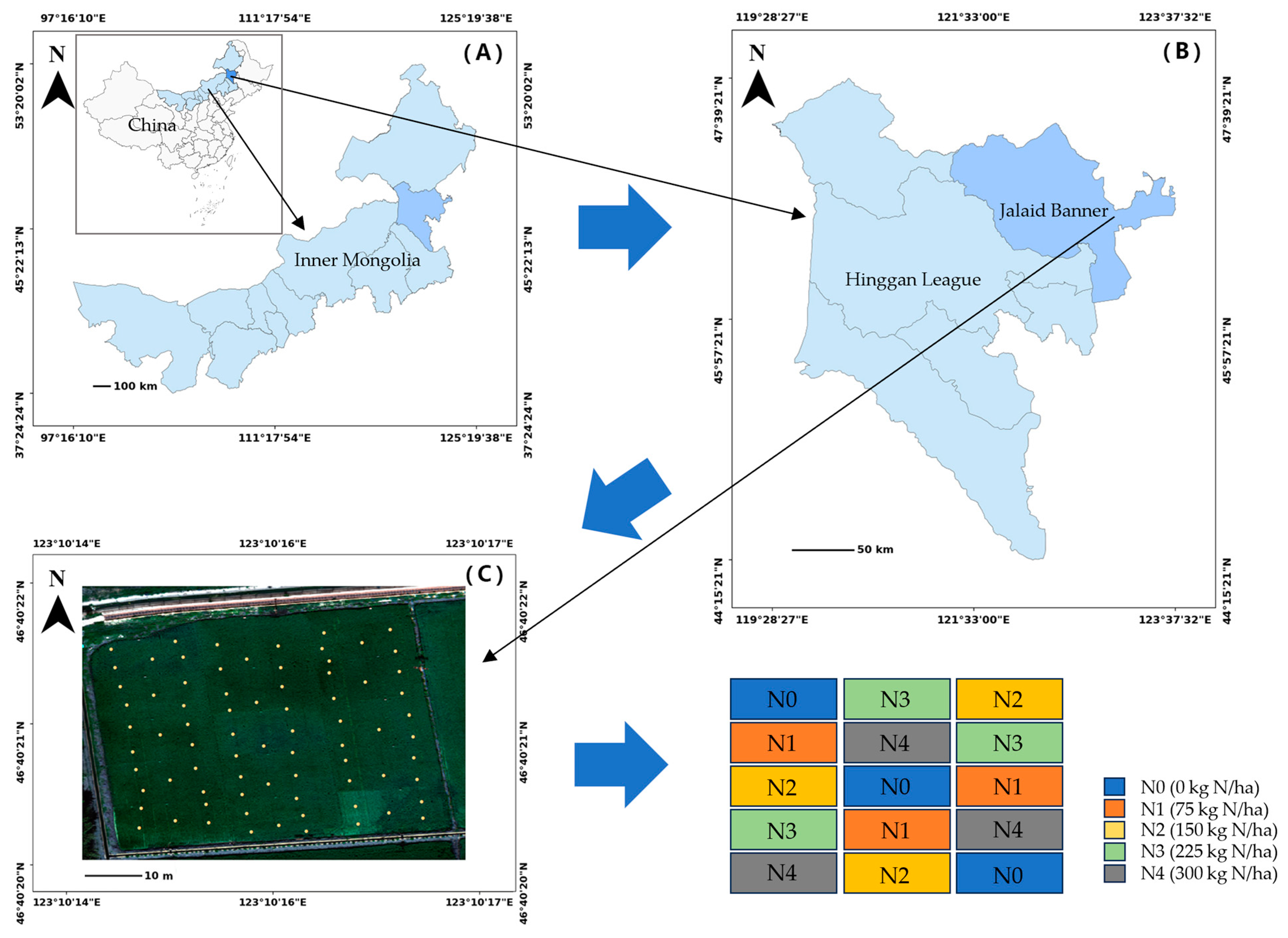
2.1. Study Area and Experimental Design

The field experiment was conducted during the 2024 rice growing season at the Jalaid Banner National Modern Agricultural Industrial Park Management Center, located in Hinggan League, Inner Mongolia, China (122°54′E, 46°44′N). This region is situated in the transitional zone between the Songnen Plain and the southern Daxing’anling Mountains, a prominent rice-producing area in northeastern China. The study area features a temperate semi-humid monsoon climate, with annual precipitation ranging from 400 to 500 mm, and a frost-free period of approximately 110–130 days. The soil type is classified as meadow black soil, which is rich in organic matter and highly suitable for paddy rice cultivation.

The rice cultivar used in this study was Zhongkefa No. 5 (japonica type), which is known for its high yield potential and strong lodging resistance. A randomized block design was employed to assess the effects of different nitrogen levels on rice growth and nitrogen status. Five nitrogen application levels were tested: N0 (0 kg N/ha), N1 (75 kg N/ha), N2 (150 kg N/ha), N3 (225 kg N/ha), and N4 (300 kg N/ha). Each treatment was replicated three times, resulting in a total of 15 plots. Each plot measured 21 m × 13 m (273 m²), as shown in Figure 1. To minimize nitrogen migration and ensure treatment independence, two rows of colored rice were planted between adjacent plots as isolation barriers. Prior to transplanting, phosphorus (P) and potassium (K) fertilizers were uniformly applied as basal fertilizers at rates that meet local agronomic standards. Nitrogen was applied post-transplanting using urea as the nitrogen source. The specific nitrogen amounts were calculated based on individual plot areas to ensure uniform application across treatments.

This experimental design was aimed at systematically evaluating rice nitrogen response under controlled conditions while simulating practical field scenarios. The combination of multiple nitrogen levels, fixed variety, and consistent plot management enhances the scientific rigor, repeatability, and relevance of this study for data-driven rice nitrogen estimation.

2.2. Ground Sampling and LNC Determination

In this study, leaf samples were collected at three critical growth stages: heading stage (5 August), early filling stage (27 August), and late filling stage (21 September). Five representative sampling points were selected within each plot, resulting in a total of 225 samples. Fully expanded functional leaves from the middle canopy of uniformly grown plants were collected and immediately sealed in paper bags to minimize moisture loss.

In the laboratory, samples were initially heated at 105 °C for 30 min to deactivate enzymes, followed by drying at 75 °C for over 48 h until a constant weight was achieved. The dried leaves were ground to pass through a 0.2 mm sieve, homogenized, and stored in sealed containers for nitrogen analysis. Nitrogen content was determined using the Kjeldahl method, with each sample analyzed in triplicate. The average of the three measurements was used for subsequent analysis to minimize experimental error.

2.3. UAV Multispectral Data Acquisition and Preprocessing

In this study, multispectral imagery was acquired using the DJI Phantom 4 Multispectral (P4M) UAV (Figure 2), which is equipped with six sensors: five narrowband multispectral sensors (blue (B), green (G), red (R), red-edge (RE), and near-infrared (NIR)) and one RGB sensor. Data acquisition was conducted at three key rice growth stages—heading (5 August), early filling (27 August), and late filling (21 September)—between 11:00 and 14:00 under clear sky and windless conditions to ensure consistent solar illumination and reduce shadow effects. The UAV was operated at a flight altitude of 50 m, with a flight speed of 1 m/s, a front overlap of 80%, and a side overlap of 70%. Under these settings, the spatial resolution of the multispectral images was approximately 2.74 cm per pixel, allowing for fine-scale detection of canopy-level variations.

Image preprocessing was conducted using PIX4Dmapper, including image stitching, geometric correction, and radiometric calibration. Radiometric correction was performed using standardized reflectance calibration panels with known reflectance values of 25%, 50%, and 75%, captured prior to each flight. This ensured the accuracy and consistency of reflectance data across flight dates and spectral bands.

Sampling regions of interest (ROIs) corresponding to field sampling locations were manually delineated in ArcMap 10.8 as polygons based on plot boundaries and then exported as shapefiles. A custom Python script developed in PyCharm 2023.3.3 was used to extract spectral reflectance values from the radiometrically calibrated imagery. Rather than extracting reflectance from a single pixel, the mean reflectance of all pixels within each ROI polygon was calculated for each spectral band. This region-based averaging approach minimizes the effects of pixel-level noise, image misalignment, and canopy heterogeneity, thereby improving the reliability of reflectance inputs used for subsequent feature construction.

The processed spectral reflectance data served as the basis for computing vegetation indices (VIs), extracting texture features (TFs), and constructing Spectral–Texture Fusion Indices (STFIs), which were then used as input variables for model development and analysis.

2.4. Feature Extraction and Construction

2.4.1. Vegetation Indices (VIs)

VIs, derived from combinations of specific spectral bands, serve as effective indicators of vegetation status and enhance the sensitivity of remote sensing data to biophysical and biochemical crop traits [22]. Guided by existing literature, 18 VIs frequently linked to nitrogen estimation were selected for analysis (

Table 1. Vegetation indices used in this paper.

Vegetation Index	Abbreviation	Formulation	References
Normalized difference vegetation index	NDVI	$(\mathrm{N}\mathrm{I}\mathrm{R}-\mathrm{R})/(\mathrm{N}\mathrm{I}\mathrm{R}+\mathrm{R})$	[23]
Normalized difference red-edge index	NDRE	$(\mathrm{N}\mathrm{I}\mathrm{R}-\mathrm{R}\mathrm{E})/(\mathrm{N}\mathrm{I}\mathrm{R}+\mathrm{R}\mathrm{E})$	[24]
Ratio of enhanced vegetation index	RERVI	$\mathrm{R}\mathrm{E}/\mathrm{R}$	[25]
Weighted difference vegetation index	WDRVI	$(0.1\times \mathrm{N}\mathrm{I}\mathrm{R}-\mathrm{R})/(0.1\times \mathrm{N}\mathrm{I}\mathrm{R}+\mathrm{R})$	[26]
Red-edge weighted difference vegetation index	REWDRVI	$(0.12\times \mathrm{N}\mathrm{I}\mathrm{R}-\mathrm{R}\mathrm{E})/(0.12\times \mathrm{N}\mathrm{I}\mathrm{R}+\mathrm{R}\mathrm{E})$	[27]
Red-edge chlorophyll index	CIRE	$\mathrm{N}\mathrm{I}\mathrm{R}/\mathrm{R}\mathrm{E}-1$	[28]
Red-edge vegetation index	REDVI	$\mathrm{N}\mathrm{I}\mathrm{R}-\mathrm{R}\mathrm{E}$	[25]
Red-edge difference vegetation index	RERDVI	$(\mathrm{N}\mathrm{I}\mathrm{R}-\mathrm{R}\mathrm{E})/\sqrt{(\mathrm{N}\mathrm{I}\mathrm{R}+\mathrm{R}\mathrm{E})}$	[27]
Red-edge optimized soil adjusted vegetation index	REOSAVI	$\begin{array}{c}1.16\times (NIR-RE)/(NIR+\\ RE+0.16)\end{array}$	[27]
Modified red-edge simple ratio	MSR_RE	$(\mathrm{N}\mathrm{I}\mathrm{R}/\mathrm{R}\mathrm{E}-1)/\sqrt{(\mathrm{N}\mathrm{I}\mathrm{R}/\mathrm{R}\mathrm{E})}+1)$	[27]
Red-edge soil adjusted vegetation index	RESAVI	$\begin{array}{c}1.5\times (NIR-RE)/(NIR+RE\\ +0.5)\end{array}$	[27]
Soil adjusted vegetation index	SAVI	$1.5\times (\mathrm{N}\mathrm{I}\mathrm{R}-\mathrm{R})/(\mathrm{N}\mathrm{I}\mathrm{R}+\mathrm{R}+0.5)$	[29]
Optimized soil adjusted vegetation index	OSAVI	$(\mathrm{N}\mathrm{I}\mathrm{R}-\mathrm{R})/(\mathrm{N}\mathrm{I}\mathrm{R}+\mathrm{R}+0.16)$	[29]
Modified simple ratio index	MSR	$(\mathrm{N}\mathrm{I}\mathrm{R}/\mathrm{R}-1)/(\sqrt{(\mathrm{N}\mathrm{I}\mathrm{R}/\mathrm{R})}+1)$	[30]
MERIS terrestrial chlorophyll index	MTCI	$(\mathrm{N}\mathrm{I}\mathrm{R}-\mathrm{R}\mathrm{E})/(\mathrm{R}\mathrm{E}-\mathrm{R})$	[31]
Difference vegetation index	DVI	$\mathrm{N}\mathrm{I}\mathrm{R}-\mathrm{R}$	[25]
Ratio vegetation index	RVI	$\mathrm{N}\mathrm{I}\mathrm{R}/\mathrm{R}$	[32]
Green-band normalized difference vegetation index	GNDVI	$(\mathrm{N}\mathrm{I}\mathrm{R}-\mathrm{G})/(\mathrm{N}\mathrm{I}\mathrm{R}+\mathrm{G})$	[33]

). Their relationships with rice LNC across critical growth stages were examined to support the construction of regression models.

2.4.2. Texture Features (TFs)

TFs are visual attribute that reflects the spatial distribution patterns within an image, independent of luminance variations. Changes in crop canopy structure can be effectively captured by analyzing the spatial relationships between neighboring pixels using texture analysis [34]. Texture features in this study were derived using the gray-level co-occurrence matrix (GLCM), a classical statistical method introduced by Haralick et al., and widely applied in remote sensing image analysis. Among the 14 standard descriptors defined by GLCM, eight representative metrics were selected: mean (MEA), variance (VAR), homogeneity (HOM), contrast (CON), dissimilarity (DIS), entropy (ENT), correlation (COR), and second moment (SEM).

Considering the five spectral bands of the P4M multispectral sensor, a total of 40 texture features (TFs) were derived (8 metrics × 5 bands). These bands include B, G, R, E (red-edge), and N (near-infrared), where “E” replaces “RE” and “N” replaces “NIR.” Each texture feature is labeled using the format metric_band (e.g., the mean of the near-infrared band is denoted as MEA_N). Reflectance images for each band are imported into ArcGIS, masked using the same regions of interest (ROIs) as those used for VI extraction, and texture features are computed for each ROI. Texture features are calculated using a 3×3 pixel sliding window, with a gray level of 64 and a pixel offset of 1. GLCMs are computed in four orientations (0°, 45°, 90°, and 135°), and the average across these orientations is used as the final value.

To eliminate edge effects, boundary values influenced by background pixels were excluded. The mean value of each ROI’s texture image was used as the representative TF value. Details of the texture metrics are listed in

Table 2. Texture metrics extracted based on the GLCM method.

Numbering	Tm	Abbreviation	Formulation	Description
1	Mean	Mea	${\displaystyle \sum _{i=0}^{\mathrm{N}-1}}{\displaystyle \sum _{j=0}^{\mathrm{N}-1}}i\times p\left(i,j\right)$	The mean value in the texture
2	Variance	Var	${\displaystyle \sum _i}{\displaystyle \sum _j}{\left(i-u\right)}^{2}p\left(i,j\right)$	The size of the texture change
3	Homogeneity	Hom	${\displaystyle \sum _i}{\displaystyle \sum _j}{\displaystyle \frac{1}{1+{\left(i-j\right)}^2}}p\left(i,j\right)$	The homogeneity of grey level in the texture
4	Contrast	Con	${\displaystyle \sum _{n=0}^{N_g-1}}{n}^2{\left\{{\displaystyle \sum _{i=1j=1}^{N_g}}{\displaystyle \sum _{j\left(i,j\right)}^{N_g}}p\left(i,j\right)\right\}}_{\left|i-j\right|=n}$	The clarity in the texture Same as contrast
5	Dissimilarity	Dis	${\displaystyle \sum _{n=1}^{N_g-1}}n{\left\{{\displaystyle \sum _{i=1}^{N_g}}{\displaystyle \sum _{j=1}^{N_g}}p\left(i,j\right)\right\}}_{\left|i-j\right|=n}$	The similarity of the pixels in the texture
6	Entropy	Ent	$-{\displaystyle \sum _i}{\displaystyle \sum _j}p\left(i,j\right)\mathrm{l}\mathrm{o}\mathrm{g}\left(p\left(i,j\right)\right)$	The diversity of the pixels in the texture
7	Second moment	Sem	${\displaystyle \sum _i}{\displaystyle \sum _j}\{p\left(i,j\right){\}}^2$	The uniformity of greyscale in the texture
8	Correlation	Cor	${\displaystyle \frac{{\displaystyle \sum _i}{\displaystyle \sum _j}\left(i,j\right)p\left(i,j\right)-{\mu }_i{\mu }_j}{{\sigma }_i{\sigma }_i}}$	The consistency in the texture

Note: The parameters $ui,uj,\sigma i$, and $\sigma j$ represent the average and standard deviation of the row and column sums of the GLCM, $i$ and $j$ represent the row and column indices, respectively, and $p$ denotes a matrix. $p\left(i,j\right)$ signifies the ratio of the value at the corresponding row and column in the matrix to the sum of all values within the matrix.

.

2.4.3. Spectral–Texture Fusion Indices (STFIs) Construction

To improve the accuracy and robustness of rice LNC estimation, this study developed a suite of STFIs by integrating spectral reflectance and texture features derived from UAV-based multispectral imagery. These indices were specifically designed to enhance the sensitivity of fused spectral–spatial features to LNC variations under complex canopy conditions.

Based on Pearson correlation analysis, the temporal dynamics of spectral and texture features across rice growth stages, and insights from previous studies, four features were selected for constructing STFIs. These include two spectral bands—RE and NIR—and two texture features—CON_E (contrast derived from the RE band) and CON_N (contrast derived from the NIR band).

To capture the complementary characteristics of spectral and spatial information, two STFIs construction strategies were adopted: the Normalized Ratio Index (R), aimed at reducing scale differences and improving robustness; and the Multiplicative Enhancement Index (M), designed to amplify synergistic interactions between features. Based on these strategies, three types of STFIs were formulated: STFI2 (two-feature indices combining one spectral and one texture feature), STFI3 (three-feature indices composed of either two spectral and one texture feature or vice versa), and STFI4 (four-feature indices integrating two spectral and two texture features for enhanced biophysical representation and nitrogen sensitivity). Each index follows a standardized naming convention:

STFI + [Number of Features] + [Computation Method: R or M] + [_Feature1] + [_Feature2] + … + [_FeatureN].

For example, STFI4R_E_CON_E_N_CON_N denotes a four-feature index calculated using the normalized ratio method and composed of red-edge reflectance, red-edge contrast, NIR reflectance, and NIR contrast. Each feature is separated by an underscore (_) to ensure clarity and consistency. This naming convention promotes interpretability, reproducibility, and consistent application across different datasets and modeling approaches. In total, 27 STFIs were constructed using the selected features, with their mathematical formulations provided below:

STFI2—Two-Feature Spectral–Texture Fusion Indices:

Normalized Ratio Index:

$$\mathrm{S}\mathrm{T}\mathrm{F}\mathrm{I}2\_\mathrm{R}={\displaystyle \frac{{\mathrm{F}}_1}{{\mathrm{F}}_2}}$$

(1)

Multiplicative Enhancement Index:

$$\mathrm{S}\mathrm{T}\mathrm{F}\mathrm{I}2\_\mathrm{M}={\mathrm{F}}_1\times {\mathrm{F}}_2$$

(2)

STFI3—Three-Feature Spectral–Texture Fusion Indices:

Normalized Ratio Index:

$$\mathrm{S}\mathrm{T}\mathrm{F}\mathrm{I}3\_\mathrm{R}={\displaystyle \frac{{\mathrm{F}}_1\times {\mathrm{F}}_2}{{\mathrm{F}}_3}}$$

(3)

Multiplicative Enhancement Index:

$$\mathrm{S}\mathrm{T}\mathrm{F}\mathrm{I}{3}_{-}\mathrm{M}={\mathrm{F}}_1\times {\mathrm{F}}_2\times {\mathrm{F}}_3$$

(4)

STFI4—Four-Feature Spectral–Texture Fusion Indices:

Normalized Ratio Index:

$$\mathrm{S}\mathrm{T}\mathrm{F}\mathrm{I}4\_\mathrm{R}={\displaystyle \frac{{\mathrm{F}}_1\times {\mathrm{F}}_2}{{\mathrm{F}}_3\times {\mathrm{F}}_4}}$$

(5)

Multiplicative Enhancement Index:

$$\mathrm{S}\mathrm{T}\mathrm{F}\mathrm{I}4\_\mathrm{M}={\mathrm{F}}_1\times {\mathrm{F}}_2\times {\mathrm{F}}_3\times {\mathrm{F}}_4$$

(6)

where R denotes the normalized ratio calculation, M denotes the multiplicative enhancement calculation, and F₁, F₂, etc., represent selected spectral or texture features.

2.5. Feature Selection Strategy

To reduce feature redundancy, enhance model generalizability, and improve prediction accuracy, a two-stage feature selection strategy was implemented in this study. First, preliminary filtering was performed using the Pearson Correlation Coefficient (PCC). Then, algorithm-specific optimization was carried out using Recursive Feature Elimination with Cross-Validation (RFECV) and Sequential Feature Selection (SFS).

The PCC was used to quantify the linear relationship between each feature and the measured LNC. The correlation coefficient $\mathrm{r}$ was calculated as follows:

$$\mathrm{r}={\displaystyle \frac{\sum (X_i-\overline{X})(Y_i-\overline{Y})}{\sqrt{\sum (X_i-\overline{X}{)}^2}\cdot \sqrt{\sum (Y_i-{\overline{Y})}^2}}}$$

(7)

where $X_i$ and $Y_i$ represent the feature value and the measured LNC, respectively, and $\overline{X}$, $\overline{Y}$ are their respective means. A high absolute $\left|\mathrm{r}\right|$ value indicates a strong correlation between the feature and LNC, making it suitable for modeling.

This two-stage feature selection framework—consisting of group-wise correlation-based filtering followed by model-specific embedded optimization—ensures that the final input variables are both statistically relevant and structurally compatible with the learning model. This approach not only reduces noise and redundancy but also enhances the interpretability, stability, and generalization ability of the regression models. The selected features were subsequently used for regression prediction and SHAP-based interpretability analysis.

2.6. Model Construction and Evaluation

This study employed four machine learning models: Random Forest (RF) [35], Support Vector Regression (SVR) [36], Extreme Gradient Boosting (XGBoost) [37], and Deep Neural Networks (DNNs) [38]. All modeling was performed using Python 3.10, scikit-learn 1.3, XGBoost 1.7, and TensorFlow 2.0.

The dataset was randomly divided into training and testing subsets at a 7:3 ratio using stratified sampling based on binned LNC distributions to ensure balanced representation of the target variable. To mitigate skewness and improve numerical stability, the LNC values were log-transformed prior to model training. After prediction, the inverse logarithmic transformation was applied to convert the estimated values back to the original LNC scale for evaluation. All input features were standardized using z-score normalization to ensure comparability and eliminate scaling bias during model training.

RF is an ensemble learning method that constructs multiple decision trees using bootstrap sampling and random feature subsets, combining the outputs through averaging to enhance prediction accuracy and reduce overfitting [35]. Similarly, XGBoost is a gradient boosting framework that incorporates regularization terms and a scalable architecture, achieving high predictive performance and robustness [37]. RFECV efficiently eliminates redundant or less informative features by performing recursive elimination, while evaluating five-fold cross-validated performance. This method ensures that only the most relevant features are retained, enhancing the model’s interpretability and performance [39]. Both RF and XGBoost models provide inherent feature importance metrics derived from node splitting criteria, making them suitable for RFECV.

SVR extends the Support Vector Machine (SVM) framework by employing an $\epsilon$-insensitive loss function and kernel mapping, allowing it to model complex nonlinear patterns in small or high-dimensional datasets [36]. However, unlike RF and XGBoost, SVR does not inherently provide feature importance metrics, particularly when using non-linear kernels such as radial basis function (RBF). While RFECV could theoretically be used with linear-kernel SVR via the model’s coef_ attribute, this was not applicable in our case due to the focus on non-linear SVR to better capture complex feature-target relationships. SFS incrementally builds the feature subset by adding variables that most improve cross-validated performance. The process continues until no further performance gain is achieved or a predefined feature number is reached [40]. Therefore, SFS was employed.

DNNs are a type of multi-layered neural network model consisting of an input layer, multiple hidden layers, and an output layer. Each layer’s nodes are connected to those in the adjacent layers, but there are no connections between nodes within the same layer. By combining fully connected layers with activation functions, DNNs automatically learn and extract hierarchical features from data, which makes them highly flexible and effective for tasks such as classification, regression, and prediction. However, similar to Support Vector Regression (SVR), DNNs do not inherently provide feature importance metrics, which can hinder the model’s interpretability. To address this, Sequential Feature Selection (SFS) was applied in this study to select the most relevant features, optimize model performance, and prevent overfitting, thus improving the model’s stability and interpretability.

Model hyperparameters were optimized using grid search combined with five-fold cross-validation. For Random Forest (RF), the candidate parameters included the number of trees (n_estimators: 50–1500), maximum tree depth (max_depth: 2–30), minimum samples required to split a node (min_samples_split: 4–60), and minimum samples required at a leaf node (min_samples_leaf: 1–40). For Support Vector Regression (SVR), the primary parameters tuned were the regularization parameter (C: 0.1–100) and ε-insensitive loss threshold (epsilon: 0.01–1). For XGBoost, the parameters optimized were the number of estimators (n_estimators: 70–150), maximum tree depth (max_depth: 2–3), learning rate (learning_rate: 0.02–0.05), subsample ratio (subsample: 0.6–0.8), column sample by tree (colsample_bytree: 0.5–0.8), and regularization terms (reg_alpha: 0.1–0.5, reg_lambda: 0.4–0.6). For Deep Neural Networks (DNNs), hyperparameters like the number of layers (model__layers: [64, 32], [128, 64], [128, 64, 32]), dropout rate (model__dropout: 0.05–0.2), L2 regularization (model__l2_reg: 0.0–0.005), batch size (batch_size: 16–32), and epochs (epochs: 150–250) were optimized. The best parameter configuration for each model and feature set was selected based on the highest average R² across folds.

To comprehensively evaluate the predictive performance of these regression models, three widely used evaluation metrics were employed: the coefficient of determination (R²), root mean square error (RMSE), and mean absolute error (MAE). R² represents the proportion of variance in the dependent variable (LNC) explained by the model and serves as a primary indicator of goodness-of-fit. It reflects how well predictions align with observed values, with values approaching 1 indicating strong agreement. RMSE quantifies prediction error by calculating the square root of the mean squared difference between estimated and actual values. As it shares the same unit as LNC (mg/g), RMSE offers an intuitive interpretation of the average prediction error. MAE computes the mean of the absolute differences between predictions and observations, also in mg/g, providing a direct assessment of model bias. Collectively, these metrics allowed for a robust and comprehensive evaluation of each model’s accuracy, robustness, and generalizability, thereby facilitating the identification of the most effective modeling strategy for rice LNC estimation.

$$R^2=1-{\displaystyle \frac{{\displaystyle {\sum }_{i=1}^n}{(y}_i-{\widehat{y}}_i{)}^2}{{\displaystyle {\sum }_{i=1}^n}{(y}_i-{\widehat{y}}_i{)}^2}}$$

(8)

$$RMSE=\sqrt{{\displaystyle \frac{{\displaystyle {\sum }_{i=1}^n}{(y}_i-{\widehat{y}}_i{)}^2}{n}}}$$

(9)

$$MAE={\displaystyle \frac{\sum |y_i-{\widehat{y}}_i|}{n}}$$

(10)

where $y_i$ and ${\widehat{y}}_i$ are the measured and predicted LNC values, $\overline{y}$ is the mean of measured LNC, and $n$ is the sample size. Higher $R^2$ and lower RMSE/MAE values indicate better model performance.

2.7. Feature Importance Interpretation Using SHAP

To evaluate the contribution of different feature types to the estimation of rice LNC, the Shapley Additive Explanations (SHAP) method was employed to analyze feature importance using three regression models—RF, SVR, and XGBoost. SHAP is grounded in cooperative game theory and calculates the marginal contribution of each feature by considering all possible feature combinations [41].

Formally, the prediction for a sample $x$ can be decomposed as

$$f\left(x\right)={\varphi }_0+{\sum }_{i=1}^M{\varphi }_i$$

(11)

where $f\left(x\right)$ is the model output, ${\varphi }_0$ is the base value (i.e., the expected model output over the training data), and ${\varphi }_i$ is the Shapley value of feature $i$, representing its individual contribution to the prediction.

Each Shapley value ${\varphi }_i$ is defined as

$${\varphi }_i={\displaystyle {\sum }_{S\subseteq N\backslash \left\{i\right\}}}{\displaystyle \frac{\left|S\right|!\left(\right|N|-|S|-1)!}{\left|N\right|!}}[f_{S\cup \left\{i\right\}}(x_{S\cup \left\{i\right\}})-f_S(x_S)]$$

(12)

where $N$ is the set of all features, $S$ is a subset of features excluding $i$, and $f_S\left(x_S\right)$ represents the model prediction based only on features in subset $S$.

Compared to traditional feature importance metrics such as mean squared error reduction or Gini impurity, SHAP offers enhanced interpretability by providing a unified framework that quantifies both the magnitude and direction of each feature’s influence on the model output. It supports both local and global interpretations, enabling the analysis of feature contributions at the level of individual predictions as well as the overall model. Furthermore, SHAP allows for consistent comparison of feature effects across different machine learning models, making it possible to fairly evaluate and interpret feature importance even when the underlying algorithms differ in structure and complexity. The overall workflow of this study is illustrated in Figure 3.

3. Results

3.1. Trend Analysis of LNC Changes

Figure 4 illustrates the distribution of measured LNC across different growth stages and nitrogen levels. The results indicated that both nitrogen application rate and phenological stage significantly affected LNC. At the heading stage, LNC values were generally high and exhibited an increasing trend with rising nitrogen input. However, this increase was not strictly linear, as LNC gains began to plateau at the highest nitrogen level. Considerable variability within treatments was also observed, particularly under high nitrogen rates, likely due to differences in nitrogen uptake efficiency or early saturation effects. During the early filling stage, LNC slightly declined across all treatments but remained elevated under moderate to high nitrogen conditions. The distribution of LNC values was more concentrated compared to the heading stage, indicating more uniform nitrogen accumulation. Although LNC continued to respond positively to nitrogen input, the marginal increase with higher rates diminished, reflecting a nonlinear response. At the late filling stage, a notable reduction in LNC was observed across all nitrogen treatments. Under high nitrogen input, LNC did not continue to increase, and in some cases even decreased, suggesting nitrogen remobilization from leaves to grains during reproductive development. In contrast, the low nitrogen treatments consistently exhibited low and narrowly distributed LNC values, indicative of prolonged nitrogen deficiency.

Overall, LNC increased with nitrogen input during the early stages but showed a nonlinear response that weakened as the crop progressed toward maturity. These results highlight the temporal dynamics of nitrogen uptake and utilization in rice, emphasizing the importance of stage-specific nitrogen management strategies to improve nitrogen use efficiency and prevent unnecessary nitrogen application in later growth stages.

Summary statistics of LNC across different growth stages are presented in

Table 3. Descriptive statistics of rice leaf nitrogen content (LNC) (unit: mg/g).

Period	Range	Mean	SD	CV (%)
Heading Stage	18.85–36.18	26.59	3.69	0.14
Early Filling Stage	11.75–30.88	21.04	4.81	0.23
Late Filling Stage	7.10–18.70	11.25	2.66	0.24

. An increasing coefficient of variation (CV) over time suggests higher variability in the later stages, which may enhance the robustness of the prediction models.

3.2. Spectral Reflectance Dynamics and Texture Feature Variation Across Rice Growth Stages

Figure 5 illustrates the mean spectral reflectance of five wavebands—B, G, R, RE, and NIR—across three rice growth stages: heading, early filling, and late filling. Across all stages, RE and NIR bands consistently exhibited higher reflectance values compared to the visible bands, with a particularly sharp increase observed during the early filling stage. At this stage, NIR reflectance exceeded 0.33, more than five times that of the B and R bands.

Reflectance trends across all bands followed a characteristic “rise–fall” pattern, peaking during early filling and declining thereafter. This temporal pattern reflects dynamic changes in canopy structure, moisture, and biochemical composition, especially as nitrogen demand and leaf expansion culminate during early filling. Among the five bands, RE and NIR showed the most pronounced sensitivity to growth stage variation, indicating their superior capacity to detect canopy condition changes during this phenological window.

These findings suggest that early filling is the most spectrally responsive period, particularly for RE and NIR wavelengths, which are known to be sensitive to leaf nitrogen and chlorophyll status. The enhanced spectral separation observed at this stage lays a critical foundation for the subsequent construction of STFIs aimed at improving LNC prediction accuracy.

Figure 6 illustrates the temporal evolution of texture features derived from UAV multispectral imagery across three critical rice growth stages: heading, early filling, and late filling. Overall, most texture features exhibited peak values at the early filling stage, indicating increased canopy heterogeneity and physiological complexity during this active growth period.

Among all texture features, CON derived from the E and N bands demonstrated the most substantial variation across stages. This was followed by HOM in the same bands. Additionally, MEA from the red-edge band also showed relatively large changes. These three features—CON, HOM, and MEA—stood out distinctly compared to other texture metrics, and all were concentrated in the red-edge and NIR spectral regions. This finding highlights the strong sensitivity of specific long-wavelength texture features to structural and physiological variations in the rice canopy.

In contrast, most other texture features—including those derived from the visible spectrum (e.g., HOM_B and CON_G)—remained relatively stable throughout the growth stages, indicating lower sensitivity to developmental changes. Similarly, other texture metrics from the red-edge and NIR bands, aside from CON, HOM, and MEA, also exhibited limited temporal variation. This suggests that only a specific subset of texture features is capable of capturing meaningful structural dynamics relevant to nitrogen status.

The pronounced variation in CON, HOM, and MEA within the red-edge and NIR bands provides a strong empirical basis for incorporating them into the construction of STFIs. Their targeted sensitivity to canopy changes reinforces their potential utility in enhancing the accuracy and robustness of LNC estimation models.

3.3. Feature Selection and Interpretability Analysis

3.3.1. Pearson Correlation Analysis

In this study, PCC was calculated to assess the linear relationships between extracted features and measured LNC. The analysis included three feature categories: VIs, TFs, and the proposed STFIs.

Although the original spectral bands exhibited relatively low correlations with LNC, several VIs constructed from these bands—particularly those involving the red-edge and near-infrared regions—demonstrated strong positive correlations. Among them, NDRE (R = 0.91, based on NIR and RE), MSR_RE (R = 0.90, based on NIR and RE), REWDRVI (R = 0.90, based on NIR and RE), RERVI (R = 0.90, based on RE and R), CIRE (R = 0.89, based on NIR and RE), and MTCI (R = 0.88, based on NIR, RE, and R) showed the highest correlations with LNC (Figure 7). These findings are consistent with previous studies indicating that most of the top-performing indices are based on RE and NIR wavelengths, which are particularly sensitive to nitrogen variations in vegetation [21].

For the TFs (Figure 8), several indices exhibited moderate correlations with LNC, highlighting the potential of spatial structural information for nitrogen estimation. The strongest positive correlation was observed for SEM_E (R = 0.67), followed by HOM_E (R = 0.39), indicating that entropy-related and homogeneity features derived from the red-edge band are particularly responsive to LNC variation. In contrast, HOM_R (R = −0.55), SEM_R (R = −0.42), and COR_R (R = −0.33) showed moderate negative correlations, suggesting that structural features derived from the red band also reflect changes associated with LNC. Additionally, ENT_E (R = −0.37) and MEA_N (R = −0.34) exhibited moderate negative correlations.

These results indicate that the texture features most sensitive to LNC primarily include SEM, HOM, ENT, MEA, and COR and are mainly derived from the RE, R, and NIR bands. This pattern reflects physiological and structural changes in the rice canopy associated with LNC variation, particularly within the longer wavelength regions, and underscores the complementary value of texture features in enhancing spectral-based LNC estimation.

Pearson correlation analysis revealed that many of the constructed STFIs exhibited strong associations with rice LNC, underscoring their effectiveness in capturing biochemical variability within the canopy.

Among all indices (Figure 9), STFI4R_E_CON_E_N_CON_N demonstrated the highest correlation with LNC (R = 0.77), followed by STFI4R_N_CON_N_E_CON_E (R = 0.71) and STFI3R_E_N_CON_E (R = 0.62). These results emphasize the utility of integrating both red-edge (RE) and near-infrared (NIR) spectral bands with texture features—particularly contrast measures (CON)—in effectively capturing nitrogen-sensitive structural and spectral characteristics. By comparison, two-feature indices such as STFI2R_N_CON_E (R = 0.52), STFI2R_E_CON_N (R = 0.51), and STFI2R_E_CON_E (R = 0.34) showed moderate correlations, suggesting that simpler spectral–texture combinations can partially reflect LNC variation, but are generally outperformed by higher-order feature fusion. further supporting the complementary nature of spectral and spatial information.

Overall, these findings demonstrate that STFIs, particularly those incorporating four fused features (STFI4R), provide a more robust and physiologically relevant means of estimating LNC compared to traditional reflectance-based indices. Importantly, the superior performance of indices involving RE and NIR features also reaffirms the critical role of these spectral regions in detecting nitrogen-related physiological status in rice canopies.

3.3.2. Feature Subset Selection and SHAP-Based Interpretability Analysis

In the first stage of feature selection, features were chosen based on their absolute correlation coefficients and statistical significance relative to LNC. Specifically, for VIs, features with an absolute correlation coefficient $\left|r\right|$ ≥ 0.4 and $p$ < 0.05 were selected. For TFs and STFIs, the selection criteria were $\left|r\right|$ ≥ 0.3 and $p$ < 0.05. As a result, the final feature subsets consisted of VIs (13 features), TFs (8 features), VIs + TFs (21 features), and STFIs (8 features).

In the second stage, model-specific embedded feature selection methods were applied. To further interpret the behavior of each model and assess the relative contribution of the selected features, SHAP analysis was conducted. SHAP values quantify the marginal contribution of each feature selected by the models to the overall model output, thereby enabling a consistent comparison of feature importance across different algorithms. Each plot displays the features retained after model-specific selection and their corresponding SHAP values. The horizontal axis represents the SHAP values (in mg/g), indicating the contribution of each feature to the model’s output. The color gradient represents the original feature values (with red indicating higher values and blue indicating lower values), illustrating how the magnitude of each feature influences the prediction outcomes.

For the VI-only configuration (Figure 10), the selected features were primarily based on red-edge and near-infrared vegetation indices. Notably, NDRE, MTCI, and RESAVI were retained by all four models. MSR_RE and WDRVI were retained by three models. Among these, NDRE made the largest contribution in all models, with MTCI also showing a relatively significant contribution.

For the TF-only configuration (Figure 11), ENT_G, MEA_N, and COR_R were retained by all four models. Among them, the features related to ENT and MEA consistently made the highest contributions across each model. These features primarily originated from the G, N, and R bands, indicating that, compared to spectral or fused features, spatial information also provided a significant contribution.

For the VI + TF configuration (Figure 12), a combination of spectral and spatial features was retained. Notably, vegetation indices such as NDRE and MTCI appeared in all four models, while REWDRVI, MSR_RE, RERVI, MEA_N, ENT_G, and COR_R were selected by three models. The consistency of these features with those retained in the VI-only and TF-only configurations highlights their significant contribution, supporting the notion that both spectral and spatial information play crucial roles in enhancing model performance.

For the STFI configuration (Figure 13), all four models retained STFI4R_E_CON_E_N_CON_N and STFI4R_E_CON_N_N_CON_E. Other fusion indices, such as STFI3R_E_N_CON_E, were selected by three models and exhibited high importance scores. These results underscore the effectiveness and generalizability of STFIs in capturing nitrogen variability across models, highlighting their robustness in representing key spectral–texture interactions.

3.4. Comparison of Model Performance Under Different Feature Sets

In this study, four regression models—RFECV-RF, RFECV-XGBoost, SFS-SVR, and SFS-DNN—were trained using the optimal feature subsets derived from each configuration. Four input configurations were tested: VIs, TFs, a combination of VIs and TFs, and STFIs. These combinations include both traditional and fused feature types. The comparison results are summarized in

Table 4. Performance evaluation of rice LNC monitoring models with different combinations of characteristics.

Feature	Model	R2	RMSE (mg/g)	MAE (mg/g)
VI	RFECV-RF	0.788	3.353	2.472
	RFECV-XGBoost	0.800	3.308	2.156
	SFS-SVR	0.805	3.208	2.143
	SFS-DNN	0.813	3.144	2.178
TF	RFECV-RF	0.706	3.949	2.845
	RFECV-XGBoost	0.789	3.395	2.432
	SFS-SVR	0.799	3.265	2.438
	SFS-DNN	0.784	3.390	2.529
VI + TF	RFECV-RF	0.801	3.247	2.327
	RFECV-XGBoost	0.829	3.040	2.263
	SFS-SVR	0.830	2.996	2.088
	SFS-DNN	0.852	2.846	1.969
STFI	RFECV-RF	0.857	2.773	1.987
	RFECV-XGBoost	0.851	2.869	2.222
	SFS-SVR	0.869	2.670	1.827
	SFS-DNN	0.874	2.621	1.845

and Figure 14. Among all configurations, the SFS-DNN model performed the best when using the STFI input, achieving the highest performance with an R² of 0.874, RMSE of 2.621 mg/g, and MAE of 1.845 mg/g, significantly outperforming the other models. The SFS-SVR, RFECV-RF, and RFECV-XGBoost models also performed well with STFI input, achieving R² values of 0.869, 0.857, and 0.851, respectively.

The VI + TF configuration also yielded good results, particularly with the SFS-DNN model, which achieved an R² of 0.852, RMSE of 2.846 mg/g, and MAE of 1.969 mg/g. Although the RMSE and MAE values were slightly higher than those of the STFI-only models.

In contrast, models trained on VI-only or TF-only inputs showed noticeably lower performance. The best R² achieved with VI-only input was 0.813 (using SFS-DNN), while the best R² for TF-only input was 0.799 (using SFS-SVR). Both configurations exhibited higher RMSE and MAE compared to the fused-feature configurations.

These results further emphasize the advantages of spectral–texture fusion features and demonstrate the superior accuracy and robustness of STFI in UAV-based rice LNC estimation tasks. Incorporating texture information into spectral indices significantly enhanced the predictive capabilities of all four models, especially in SFS-DNN.

3.5. Spatial Inversion of Rice LNC

Figure 15 presents the spatial distribution maps of rice LNC estimated using the optimal STFIs at different growth stages. Clear spatial heterogeneity in LNC was observed across the experimental area, particularly during the heading and early filling stages. Higher LNC levels were predominantly concentrated in plots with higher nitrogen input, reflecting the strong spatial sensitivity of STFIs to nitrogen variation. At the late filling stage, the overall LNC level declined significantly and spatial variability was substantially reduced. This trend aligns with the physiological dynamics of rice development, during which nitrogen remobilization and redistribution occur toward grain filling.

These inversion maps provide an intuitive and informative visualization of the spatial patterns of LNC across key phenological stages, supporting precision nitrogen management and spatially targeted interventions. The results further demonstrate the effectiveness of STFIs in capturing both spectral and structural information relevant to nitrogen estimation.

4. Discussion

4.1. Advantages of Spectral–Texture Fusion Indices (STFIs)

Canopy spectral reflectance offers integrated insights into the nitrogen status of the entire plant and plays a particularly important role in nitrogen management for rice and wheat production [32]. However, multiple interfering factors—such as vegetation biophysical traits, canopy structure, soil background, and atmospheric conditions—can obscure the spectral signal related to plant nitrogen levels, thereby reducing the accuracy of nitrogen estimation based on raw spectral reflectance [42]. To overcome these limitations, VIs constructed from R, RE, and NIR bands—such as NDVI, NDRE, and MSR_RE—are widely used to enhance sensitivity to chlorophyll and nitrogen-related variations [21,43]. Nevertheless, under conditions such as dense canopy coverage, high nitrogen application rates, or late growth stages, spectral reflectance tends to saturate, diminishing its responsiveness to subtle changes in nitrogen status [44]. As a result, the predictive performance of VIs may also be constrained under these circumstances.

In parallel, texture features extracted from the GLCM provide complementary spatial information by describing canopy arrangement, uniformity, and structural heterogeneity [45]. It has been demonstrated that incorporating texture metrics can enhance the estimation of plant traits by capturing canopy morphological characteristics that may not be fully revealed by spectral information alone [46]. In both our study and previous research, TFs such as HOM, CON, ENT, and MEA showed significant correlations with LNC [44,47], particularly during early growth stages, when canopy structure is tightly linked to nutrient availability. These texture metrics reflect spatial patterns in canopy structure, such as leaf distribution and density, which are influenced by nitrogen availability through their effects on leaf growth, tillering, and canopy closure [44,47].

Although combining VIs and TFs as independent inputs has become a common modeling practice [46,48], prior studies generally treated spectral and texture features as parallel variables without achieving deeper feature-level integration. Consistent with observations by Freitas et al. [49] and Zhang et al. [50], the simple concatenation of feature types often fails to fully exploit their synergistic potential. In contrast, the novelty of this study lies in the mathematical construction of STFIs that tightly integrate spectral reflectance and texture metrics through normalized ratio and multiplicative operations. This approach aggregates complementary biochemical and spatial information into unified descriptors, thereby enabling more detailed biophysical interpretation by explicitly capturing the interactions between specific spectral bands and associated textural properties. Such feature-level fusion reduces redundancy, improves model interpretability, and enhances prediction accuracy compared to conventional parallel feature stacking.

Among the 27 developed STFIs, indices such as STFI4R_E_CON_E_N_CON_N and STFI4R_E_CON_N_N_CON_E consistently emerged as top contributors across the RF, XGBoost, SVR, and DNN models, as revealed by SHAP global importance analyses. Their stable and robust contributions highlight the advantage of deeply integrated spectral–textural features for UAV-based LNC prediction across different modeling approaches.

Overall, these findings are in line with previous research indicating that the integration of spectral and spatial information substantially improves the prediction of crop biophysical traits. However, unlike most previous studies, which simply stacked features, this study advances the methodology by constructing mathematically integrated indices. This deeper fusion offers a more efficient, interpretable, and scalable framework for UAV-based precision nitrogen management.

4.2. Comparative Analysis of Regression Algorithms

This study utilized four regression algorithms—RF, XGBoost, SVR, and a DNN—to assess the prediction capability of various feature combinations for rice LNC. As demonstrated in the experimental results, model performance varied significantly across both algorithms and feature configurations. Among all configurations, the DNN consistently achieved the highest prediction accuracy, except when using the TF feature combination. When using the STFI-only input, SVR also performed well with an R² of 0.869 and an RMSE of 2.670 mg/g, but was slightly outperformed by DNN. RF and XGBoost also performed well with STFI input, though their performance was slightly lower compared to the DNN and SVR.

Deep Neural Networks (DNNs) are increasingly recognized in remote sensing for their ability to model complex feature interactions and nonlinearities, making them ideal for tasks that integrate spectral and texture features. This aligns with Peng et al. [14], who found that DNNs, trained with multispectral data, effectively captured intricate relationships, significantly enhancing nitrogen content predictions.

Previous studies have similarly reported that SVR performs exceptionally well in small-sample, high-dimensional, and nonlinear environments. For instance, Zhu et al. [51] and Liu et al. [52] demonstrated that SVR, based on the principle of structural risk minimization, outperformed other machine learning algorithms in complex crop monitoring tasks involving spectral and texture information. Moreover, Li et al. [53] confirmed that SVR achieved higher prediction accuracy when texture features were included, further validating its strength in handling heterogeneous canopy structures across different growth stages.

Meanwhile, Random Forest (RF) has been widely recognized for its ensemble-based robustness and noise tolerance. Previous research by Li et al. [53] and other scholars [47,54] emphasized that RF maintains strong stability and interpretability, particularly in trait estimation tasks using spectral features. While the performance of RF was marginally lower than that of SVR, it demonstrated stable generalization capability. This observation aligns with Yu et al. [55], who noted that RF effectively mitigates overfitting and performs robustly across heterogeneous datasets.

As for Extreme Gradient Boosting (XGBoost), although it is valued for its fast convergence, strong mathematical interpretability, and scalability, its performance was relatively lower under the current experimental conditions. This may be attributed to its reliance on larger sample sizes for optimal training, as previously suggested by Oliveira [47] and demonstrated in studies involving feature selection with XGBoost [56]. Nevertheless, XGBoost’s advantages, including rapid model training and efficient feature ranking, indicate its potential for future applications if larger datasets or more advanced tuning strategies are adopted.

In line with previous studies, this research confirms that a DNN, when paired with optimized STFIs, delivers the highest prediction accuracy. While SVR, RF, and XGBoost also performed well with STFIs, the DNN proved to be the most effective in integrating complex spectral and texture features, making it the optimal choice for precise rice leaf nitrogen content estimation.

4.3. Benefits of the Two-Stage Feature Selection and SHAP Interpretability

To enhance model robustness and mitigate feature redundancy, a two-stage feature selection strategy was implemented. As Wu et al. [44] demonstrated, RFECV effectively integrates recursive feature elimination with cross-validation, enabling the automatic determination of optimal feature numbers and combinations, thereby enhancing model stability and generalization. Meanwhile, Zhang and Xue [57] reported that SFS adopts a stepwise forward selection strategy, incrementally adding features based on predictive performance improvements, making it particularly suitable for moderate-sized datasets and minimizing overfitting risks. This two-stage approach effectively constructed compact yet informative feature subsets tailored to the requirements of each regression model.

Following feature selection, SHAP (SHapley Additive exPlanations) analysis was employed to evaluate the global importance of individual features. According to Lundberg and Lee [41], SHAP, grounded in cooperative game theory, ensures a fair and consistent allocation of feature contributions across different models. Unlike traditional feature importance measures, SHAP offers a theoretically sound framework for interpreting the contributions of each feature even when multicollinearity or complex interactions are present.

In this study, the SHAP summary plots revealed the feature selection patterns across different models. Under the STFI combination, SHAP analysis consistently highlighted STFI4R_E_CON_E_CON_N and STFI4R_E_CON_N_CON_E as the major contributors across all models, thus validating the reliability of the feature selection process. Additionally, in the VI, TF, and VI + TF configurations, the features selected by SHAP were also highly correlated with riceLNC.

Importantly, recent research emphasized that combining machine learning models with interpretability tools such as SHAP significantly improves the transparency and credibility of predictive modeling processes. As Bzdok et al. [58] pointed out, in UAV-based high-dimensional datasets, enhancing model interpretability is critical for bridging data-driven predictions with domain-specific agronomic understanding. In agricultural remote sensing applications, explainable AI frameworks are increasingly recognized as essential for supporting reliable decision-making [58].

Overall, the combination of a structured two-stage feature selection pipeline and post hoc SHAP analysis proved highly effective in identifying stable, high-impact features and improving model interpretability. These results validate both the methodological framework and the pivotal role of Spectral–Texture Fusion Indices in advancing the precision of rice nitrogen content monitoring.

4.4. Limitations and Future Perspectives

This study conducted multi-temporal UAV observations across three critical growth stages; however, all data were collected within a single cropping season. Therefore, the generalizability of the results to multiple years, different rice varieties, or varying environmental conditions requires further comprehensive evaluation.

To support broader applicability, a long-term experimental platform is being established, with continuous data collection across multiple seasons. The goal is to develop a multi-year, multi-season, and multi-variety dataset that will facilitate comprehensive validation under diverse environmental and management conditions. Future research will focus on extending this framework to different regions and rice varieties, incorporating additional remote sensing modalities—such as hyperspectral and thermal imagery—and exploring advanced modeling approaches to further improve prediction accuracy and model adaptability.

5. Conclusions

Accurate estimation of rice LNC is critical for optimizing nitrogen management in precision agriculture. This study presents a UAV-based framework for LNC estimation that integrates spectral and texture features through the development of STFIs. By leveraging these STFIs, we examined their effectiveness in enhancing model performance using four regression algorithms: RF, XGBoost, SVR, and DNNs. Our results consistently demonstrate that STFIs outperform traditional VI, TF, and their combination (VI + TF) across all models. Among the four models, the SFS-DNN model with STFI features achieved the highest prediction accuracy, with an R² of 0.874 and an RMSE of 2.621 mg/g, surpassing the performance of RF, XGBoost, and SVR. This result underscores the exceptional ability of DNNs to capture complex nonlinear relationships within high-dimensional feature spaces. Furthermore, SHAP analysis revealed that STFIs, particularly STFI4R_E_CON_E_N_CON_N and STFI4R_E_CON_N_N_CON_E, played significant roles in model predictions, further emphasizing the importance of integrating both spectral and texture information. The framework also highlighted the potential of UAV-based LNC monitoring to enhance nitrogen management at the field scale, enabling more accurate and robust predictions. By combining STFIs with advanced machine learning techniques such as DNNs, this study offers valuable insights into optimizing nitrogen fertilizer applications in rice cultivation.

Overall, this study demonstrates the advantages of integrating spectral–texture fusion features with DNNs for UAV-based LNC estimation. The proposed method offers a scalable, accurate, and interpretable approach for precision agriculture, with promising potential for further advancements through multi-season, multi-region validation and the exploration of additional sensor modalities.

References

1. Muthayya, S.; Sugimoto, J.D.; Montgomery, S.; Maberly, G.F. An overview of global rice production, supply, trade, and consumption. Ann. N. Y. Acad. Sci. 2014, 1324, 7–14. [Google Scholar] [CrossRef] [PubMed]
2. Zheng, H.B.; Ma, J.F.; Zhou, M.; Li, D.; Yao, X.; Cao, W.X.; Zhu, Y.; Cheng, T. Enhancing the nitrogen signals of rice canopies across critical growth stages through the integration of textural and spectral information from unmanned aerial vehicle (UAV) multispectral imagery. Remote Sens. 2020, 12, 957. [Google Scholar] [CrossRef]
3. Xu, S.Z.; Xu, X.A.; Blacker, C.; Gaulton, R.; Zhu, Q.Z.; Yang, M.; Yang, G.J.; Zhang, J.M.; Yang, Y.A.; Yang, M.; et al. Estimation of leaf nitrogen content in rice using vegetation indices and feature variable optimization with information fusion of multiple-sensor images from UAV. Remote Sens. 2023, 15, 854. [Google Scholar] [CrossRef]
4. Zhu, Y.; Liu, J.; Tao, X.; Su, X.; Li, W.; Zha, H.; Wu, W.; Li, X. A Three-Dimensional Conceptual Model for Estimating the Above-Ground Biomass of Winter Wheat Using Digital and Multispectral Unmanned Aerial Vehicle Images at Various Growth Stages. Remote Sens. 2023, 15, 3332. [Google Scholar] [CrossRef]
5. Wang, W.; Zheng, H.; Wu, Y.; Yao, X.; Zhu, Y.; Cao, W.; Cheng, T. An assessment of background removal approaches for improved estimation of rice leaf nitrogen concentration with unmanned aerial vehicle multispectral imagery at various observation times. Field Crop. Res. 2022, 283, 108543. [Google Scholar] [CrossRef]
6. Wang, K.; Shan, S.; Dou, W.; Wei, H.; Zhang, K. A cross-modal deep learning method for enhancing photovoltaic power forecasting with satellite imagery and time series data. Energy Convers. Manag. 2025, 323, 119218. [Google Scholar] [CrossRef]
7. Dong, H.; Dong, J.; Sun, S.; Bai, T.; Zhao, D.; Yin, Y.; Shen, X.; Wang, Y.; Zhang, Z.; Wang, Y. Crop water stress detection based on UAV remote sensing systems. Agric. Water Manag. 2024, 303, 109059. [Google Scholar] [CrossRef]
8. Wu, G.; Al-qaness, M.A.A.; Al-Alimi, D.; Dahou, A.; Abd Elaziz, M.; Ewees, A.A. Hyperspectral image classification using graph convolutional network: A comprehensive review. Expert Syst. Appl. 2024, 257, 125106. [Google Scholar] [CrossRef]
9. Segarra, J.; Rezzouk, F.Z.; Aparicio, N.; González-Torralba, J.; Aranjuelo, I.; Gracia-Romero, A.; Araus, J.L.; Kefauver, S.C. Multiscale assessment of ground, aerial and satellite spectral data for monitoring wheat grain nitrogen content. Inf. Process. Agric. 2023, 10, 504–522. [Google Scholar] [CrossRef]
10. Flynn, K.C.; Witt, T.W.; Baath, G.S.; Chinmayi, H.K.; Smith, D.R.; Gowda, P.H.; Ashworth, A.J. Hyperspectral reflectance and machine learning for multi-site monitoring of cotton growth. Smart Agric. Technol. 2024, 9, 100536. [Google Scholar] [CrossRef]
11. Guo, Y.H.; Wang, H.X.; Wu, Z.F.; Wang, S.X.; Sun, H.Y.; Senthilnath, J.; Wang, J.Z.; Bryant, C.R.; Fu, Y.S. Modified Red Blue Vegetation Index for Chlorophyll Estimation and Yield Prediction of Maize from Visible Images Captured by UAV. Sensors 2020, 20, 5055. [Google Scholar] [CrossRef] [PubMed]
12. Jiang, X.T.; Gao, L.T.; Xu, X.; Wu, W.B.; Yang, G.J.; Meng, Y.; Feng, H.K.; Li, Y.F.; Xue, H.Y.; Chen, T.E. Combining UAV remote sensing with ensemble learning to monitor leaf nitrogen content in custard apple (Annona squamosa L.). Agronomy 2025, 15, 38. [Google Scholar] [CrossRef]
13. Lu, J.; Cheng, D.; Geng, C.; Zhang, Z.; Xiang, Y.; Hu, T. Combining plant height, canopy coverage and vegetation index from UAV-based RGB images to estimate leaf nitrogen concentration of summer maize. Biosyst. Eng. 2021, 202, 42–54. [Google Scholar] [CrossRef]
14. Peng, Y.P.; Zhong, W.L.; Peng, Z.P.; Tu, Y.T.; Xu, Y.G.; Li, Z.X.; Liang, J.Y.; Huang, J.C.; Liu, X.; Fu, Y.Q. Enhanced estimation of rice leaf nitrogen content via the integration of hybrid preferred features and deep learning methodologies. Agronomy 2024, 14, 1248. [Google Scholar] [CrossRef]
15. Li, M.H.; Liu, Y.; Lu, X.; Jiang, J.L.; Ma, X.H.; Wen, M.; Ma, F.Y. Integrating unmanned aerial vehicle-derived vegetation and texture indices for the estimation of leaf nitrogen concentration in drip-irrigated cotton under reduced nitrogen treatment and different plant densities. Agronomy 2024, 14, 120. [Google Scholar] [CrossRef]
16. Gupta, S.K.; Pandey, A.C. Spectral aspects for monitoring forest health in extreme season using multispectral imagery. Egypt. J. Remote Sens. Space Sci. 2021, 24, 579–586. [Google Scholar] [CrossRef]
17. Yang, H.; Hu, Y.; Zheng, Z.; Qiao, Y.; Zhang, K.; Guo, T.; Chen, J. Estimation of Potato Chlorophyll Content from UAV Multispectral Images with Stacking Ensemble Algorithm. Agronomy 2022, 12, 2318. [Google Scholar] [CrossRef]
18. Miao, H.L.; Zhang, R.; Song, Z.H.; Chang, Q.R. Estimating Winter Wheat Canopy Chlorophyll Content Through the Integration of Unmanned Aerial Vehicle Spectral and Textural Insights. Remote Sens. 2025, 17, 406. [Google Scholar] [CrossRef]
19. Yue, J.; Yang, G.; Tian, Q.; Feng, H.; Xu, K.; Zhou, C. Estimate of winter-wheat above-ground biomass based on UAV ultrahigh-ground-resolution image textures and vegetation indices. ISPRS J. Photogramm. Remote Sens. 2019, 150, 226–244. [Google Scholar] [CrossRef]
20. Zheng, H.; Cheng, T.; Zhou, M.; Li, D.; Yao, X.; Tian, Y.; Cao, W.; Zhu, Y. Improved estimation of rice aboveground biomass combining textural and spectral analysis of UAV imagery. Precis. Agric. 2018, 20, 611–629. [Google Scholar] [CrossRef]
21. Su, X.; Nian, Y.; Yue, H.; Zhu, Y.; Li, J.; Wang, W.; Sheng, Y.; Ma, Q.; Liu, J.; Wang, W.; et al. Improving wheat leaf nitrogen concentration (LNC) estimation across multiple growth stages using feature combination indices (FCIs) from UAV multispectral imagery. Agronomy 2024, 14, 1052. [Google Scholar] [CrossRef]
22. Yao, X.; Zhu, Y.; Tian, Y.; Feng, W.; Cao, W. Exploring hyperspectral bands and estimation indices for leaf nitrogen accumulation in wheat. Int. J. Appl. Earth Obs. Geoinf. 2010, 12, 89–100. [Google Scholar] [CrossRef]
23. Rouse, J.W.; Haas, R.H.; Schell, J.A.; Deering, D.W. Monitoring vegetation systems in the Great Plains with ERTS. Nasa Spec. Publ. 1974, 351, 309. [Google Scholar]
24. Gitelson, A.A.; Merzlyak, M.N. Quantitative Estimation of Chlorophyll-a Using Reflectance Spectra: Experiments with Autumn Chestnut and Maple Leaves. J. Photochem. Photobiol. 1994, 22, 247–252. [Google Scholar] [CrossRef]
25. Tucker, C.J. Red and Photographic Infrared Linear Combinations for Monitoring Vegetation. Remote Sens. Environ. 1979, 8, 127–150. [Google Scholar] [CrossRef]
26. Gitelson, A.A. Wide Dynamic Range Vegetation Index for Remote Quantification of Biophysical Characteristics of Vegetation. J. Plant Physiol. 2004, 161, 165–173. [Google Scholar] [CrossRef] [PubMed]
27. Cao, Q.; Miao, Y.; Wang, H.; Huang, S.; Cheng, S.; Khosla, R.; Jiang, R. Non-Destructive Estimation of Rice Plant Nitrogen Status with Crop Circle Multispectral Active Canopy Sensor. F. Crop. Res. 2013, 154, 133–144. [Google Scholar] [CrossRef]
28. Gitelson, A.A.; Viña, A.; Ciganda, V.; Rundquist, D.C.; Arkebauer, T.J. Remote Estimation of Canopy Chlorophyll Content in Crops. Geophys. Res. Lett. 2005, 32, 7. [Google Scholar] [CrossRef]
29. Rondeaux, G.; Steven, M.; Baret, F. Optimization of Soil-Adjusted Vegetation Indices. Remote Sens. Environ. 1996, 55, 95–107. [Google Scholar] [CrossRef]
30. Chen, J.M. Evaluation of Vegetation Indices and a Modified Simple Ratio for Boreal Applications. Can. J. Remote Sens. 1996, 22, 229–242. [Google Scholar] [CrossRef]
31. Dash, J.; Curran, P.J. The MERIS terrestrial chlorophyll index. Int. J. Remote Sens. 2004, 25, 5403–5413. [Google Scholar] [CrossRef]
32. Zhu, Y.; Yao, X.; Tian, Y.; Liu, X.; Cao, W. Analysis of common canopy vegetation indices for indicating leaf nitrogen accumulations in wheat and rice. Int. J. Appl. Earth Obs. Geoinf. 2008, 10, 1–10. [Google Scholar] [CrossRef]
33. Gitelson, A.; Kaufman, Y.J.; Merzlyak, M.N. Use of a green channel in remote sensing of global vegetation from EOS-MODIS. Remote Sens. Environ. 1996, 58, 289–298. [Google Scholar] [CrossRef]
34. Zhou, M.; Zheng, H.; He, C.; Liu, P.; Awan, G.M.; Wang, X.; Cheng, T.; Zhu, Y.; Cao, W.; Yao, X. Wheat phenology detection with the methodology of classification based on the time-series UAV images. Field Crop. Res. 2023, 292, 108798. [Google Scholar] [CrossRef]
35. Shao, G.; Han, W.; Zhang, H.; Liu, S.; Wang, Y.; Zhang, L.; Cui, X. Mapping maize crop coefficient Kc using random forest algorithm based on leaf area index and UAV-based multispectral vegetation indices. Agric. Water Manag. 2021, 252, 106906. [Google Scholar] [CrossRef]
36. Wu, Z.; Luo, J.; Rao, K.; Lin, H.; Song, X. Estimation of wheat kernel moisture content based on hyperspectral reflectance and satellite multispectral imagery. Int. J. Appl. Earth Obs. Geoinf. 2024, 126, 103597. [Google Scholar] [CrossRef]
37. Chen, T.; Guestrin, C. Xgboost: A scalable tree boosting system. In Proceedings of the 22nd ACM Sigkdd International Conference on Knowledge Discovery and Data Mining, San Francisco, CA, USA, 13–17 August 2016. [Google Scholar]
38. Gao, M.; Huang, X.Y.; Wang, F.; Zhang, H.L.; Zhao, H.X.; Gao, X.Y. Sea Surface Salinity Inversion Based on DNN Model. Adv. Mar. Sci. 2022, 40, 496–504. [Google Scholar]
39. Wang, C.H.; Xiao, Z.Y.; Wu, J.H. Functional connectivity-based classification of autism and control using SVM-RFECV on rs-fMRI data. Phys. Med. 2019, 65, 99–105. [Google Scholar] [CrossRef] [PubMed]
40. Uncu, Ö.; Türkşen, I.B. A Novel Feature Selection Approach: Combining Feature Wrappers and Filters. Inf. Sci. 2007, 177, 449–466. [Google Scholar] [CrossRef]
41. Lundberg, S.M.; Lee, S.-I. A Unified Approach to Interpreting Model Predictions. Adv. Neural Inf. Process. Syst. 2017, 30, 4765–4774. [Google Scholar]
42. Dorigo, W.A.; Zurita-Milla, R.; de Wit, A.J.W.; Brazile, J.; Singh, R.; Schaepman, M.E. A Review on Reflective Remote Sensing and Data Assimilation Techniques for Enhanced Agroecosystem Modeling. Int. J. Appl. Earth Obs. Geoinf. 2007, 9, 165–193. [Google Scholar] [CrossRef]
43. Thenkabail, P.S.; Smith, R.B.; De Pauw, E. Hyperspectral Vegetation Indices and Their Relationships with Agricultural Crop Characteristics. Remote Sens. Environ. 2000, 71, 158–182. [Google Scholar] [CrossRef]
44. Wu, J.; Zheng, D.; Wu, Z.; Song, H.; Zhang, X. Prediction of buckwheat maturity in UAV-RGB images based on recursive feature elimination cross-validation: A case study in Jinzhong, Northern China. Plants 2022, 11, 3257. [Google Scholar] [CrossRef] [PubMed]
45. Liu, J.; Zhu, Y.; Song, L.; Su, X.; Li, J.; Zheng, J.; Zhu, X.; Ren, L.; Wang, W.; Li, X. Optimizing window size and directional parameters of GLCM texture features for estimating rice AGB based on UAVs multispectral imagery. Front. Plant Sci. 2023, 14, 1284235. [Google Scholar] [CrossRef] [PubMed]
46. Wang, F.; Yi, Q.; Hu, J.; Xie, L.; Yao, X.; Xu, T.; Zheng, J. Combining spectral and textural information in UAV hyperspectral images to estimate rice grain yield. Int. J. Appl. Earth Obs. Geoinf. 2021, 102, 102397. [Google Scholar] [CrossRef]
47. Li, Z.; Zhou, X.; Cheng, Q.; Fei, S.; Chen, Z. A Machine-Learning Model Based on the Fusion of Spectral and Textural Features from UAV Multi-Sensors to Analyse the Total Nitrogen Content in Winter Wheat. Remote Sens. 2023, 15, 2152. [Google Scholar] [CrossRef]
48. Shu, M.Y.; Wang, Z.Y.; Guo, W.; Qiao, H.B.; Fu, Y.Y.; Guo, Y.; Wang, L.G.; Ma, Y.T.; Gu, X.H. Effects of Variety and Growth Stage on UAV Multispectral Estimation of Plant Nitrogen Content of Winter Wheat. Agriculture 2024, 14, 1775. [Google Scholar] [CrossRef]
49. Freitas, R.G.; Pereira, F.R.; Dos Reis, A.A.; Magalhães, P.S.; Figueiredo, G.K.; Do Amaral, L.R. Estimating pasture aboveground biomass under an integrated crop-livestock system based on spectral and texture measures derived from UAV images. Comput. Electron. Agric. 2022, 198, 107122. [Google Scholar] [CrossRef]
50. Zhang, X.; Zhang, K.; Sun, Y.; Zhao, Y.; Zhuang, H.; Ban, W.; Chen, Y.; Fu, E.; Chen, S.; Liu, J.; et al. Combining spectral and texture features of UAS-based multispectral images for maize leaf area index estimation. Remote Sens. 2022, 14, 331. [Google Scholar] [CrossRef]
51. Zhu, W.; Feng, Z.; Dai, S.; Zhang, P.; Wei, X. Using UAV multispectral remote sensing with appropriate spatial resolution andmachine learning to monitor wheat scab. Agriculture 2022, 12, 1785. [Google Scholar] [CrossRef]
52. Camps-Valls, G.; Bruzzone, L.; Rojo-Álvarez, J.L.; Melgani, F. Robust support vector regression for biophysical variable estimation from remotely sensed images. IEEE Geosci. Remote Sens. Lett. 2006, 3, 339–343. [Google Scholar] [CrossRef]
53. Li, R.; Wang, D.; Zhu, B.; Liu, T.; Sun, C.; Zhang, Z. Estimation of nitrogen content in wheat using indices derived from RGB and thermal infrared imaging. Field Crop. Res. 2022, 289, 108735. [Google Scholar] [CrossRef]
54. Li, Z.; Chen, Z.; Cheng, Q.; Duan, F.; Sui, R.; Huang, X.; Xu, H. UAV-based hyperspectral and ensemble machine learning for predicting yield in winter wheat. Agronomy 2022, 12, 202. [Google Scholar] [CrossRef]
55. Metz, M.; Abdelghafour, F.; Roger, J.; Lesnoff, M. A novel robust PLS regression method inspired from boosting principles: RoBoost-PLSR. Anal. Chim. Acta 2021, 1179, 338823. [Google Scholar] [CrossRef] [PubMed]
56. Samat, A.; Li, E.; Wang, W.; Liu, S.; Lin, C.; Abuduwaili, J. Meta-XGBoost for hyperspectral image classification using extended MSER-guided morphological profiles. Remote Sens. 2020, 12, 1973. [Google Scholar] [CrossRef]
57. Guyon, I.; Elisseeff, A. An Introduction to Variable and Feature Selection. J. Mach. Learn. Res. 2003, 3, 1157–1182. [Google Scholar]
58. Bzdok, D.; Altman, N.; Krzywinski, M. Statistics versus Machine Learning. Nat. Methods 2018, 15, 233–234. [Google Scholar] [CrossRef] [PubMed]
Figure 1. Study location and field experimental layout. (A) Inner Mongolia Autonomous Region. (B) Hinggan League. (C) Experimental field in Jalaid Banner, showing five nitrogen treatment levels (N1–N5) distributed across 15 randomized plots.
Remotesensing 17 02499 g001
Figure 2. Multispectral UAVs and sensors.
Remotesensing 17 02499 g002
Figure 3. Overall workflow of this study.
Remotesensing 17 02499 g003
Figure 4. Distribution of LNC under different nitrogen application rates (0–300 kg N/ha) across three rice growth stages. (a) Heading stage. (b) Early filling stage. (c) Late filling stage.
Remotesensing 17 02499 g004
Figure 5. Mean spectral reflectance of rice canopy across growth stages.
Remotesensing 17 02499 g005
Figure 6. Texture features of rice canopy across growth stages.
Remotesensing 17 02499 g006
Figure 7. Spectral band and VI correlation heat map.
Remotesensing 17 02499 g007
Figure 8. TF correlation heat map.
Remotesensing 17 02499 g008
Figure 9. STFI correlation heat map.
Remotesensing 17 02499 g009
Figure 10. SHAP plots of selected features for different models using VI feature combinations. Panels (a) represent RF, (b) XGBoost, (c) SVR, and (d) DNN, respectively.
Remotesensing 17 02499 g010
Figure 11. SHAP plots of selected features for different models using TF feature combinations. Panels (a) represent RF, (b) XGBoost, (c) SVR, and (d) DNN, respectively.
Remotesensing 17 02499 g011
Figure 12. SHAP plots of selected features for different models using VI + TF feature combinations. Panels (a) represent RF, (b) XGBoost, (c) SVR, and (d) DNN, respectively.
Remotesensing 17 02499 g012
Figure 13. SHAP plots of selected features for different models using STFI feature combinations. Panels (a) represent RF, (b) XGBoost, (c) SVR, and (d) DNN, respectively.
Remotesensing 17 02499 g013
Figure 14. Model inversion results using four regression algorithms (RF, XGBoost, SVR, and DNN) across four feature combinations (VI, TF, VI + TF, and STFI), with rows representing feature combinations and columns representing machine learning models.
Remotesensing 17 02499 g014
Figure 15. Spatial distribution of estimated LNC at three stages. (a) Heading stage. (b) Early filling stage. (c) Late filling stage.
Remotesensing 17 02499 g015