Abstract
Accurate crop yield prediction is essential for stabilizing food supply chains and reducing the uncertainties in financial risks related to agricultural production. Yet, it is even more essential to understand how crop yield models make predictions depending on their relationship to Earth Observation (EO) indicators. This study presents a state-of-the-art explainable artificial intelligence (XAI) method to estimate corn yield prediction over the Corn Belt in the continental United States (CONUS). We utilize the recently introduced Kolmogorov–Arnold Network (KAN) architecture, which offers an interpretable alternative to the traditional Multi-Layer Perceptron (MLP) approach by utilizing learnable spline-based activation functions instead of fixed ones. By including a KAN in our crop yield prediction framework, we are able to achieve high prediction accuracy and identify the temporal drivers behind crop yield variability. We create a multi-source dataset that includes biophysical parameters along the crop phenology, as well as meteorological, topographic, and soil parameters to perform end-of-season and in-season predictions of county-level corn yields between 2016–2023. The performance of the KAN model is compared with the commonly used traditional machine learning (ML) models and its architecture-wise equivalent MLP. The KAN-based crop yield model outperforms the other models, achieving an R2 of 0.85, an RMSE of 0.84 t/ha, and an MAE of 0.62 t/ha (compared to MLP: R2 = 0.81, RMSE = 0.95 t/ha, and MAE = 0.71 t/ha). In addition to end-of-season predictions, the KAN model also proves effective for in-season yield forecasting. Notably, even three months prior to harvest, the KAN model demonstrates strong performance in in-season yield forecasting, achieving an R2 of 0.82, an MAE of 0.74 t/ha, and an RMSE of 0.98 t/ha. These results indicate that the model maintains a high level of explanatory power relative to its final performance. Overall, these findings highlight the potential of the KAN model as a reliable tool for early yield estimation, offering valuable insights for agricultural planning and decision-making.
1. Introduction
Food security is threatened by a number of factors globally. The rise in the global population and the reduction in arable land due to soil degradation caused by excessive fertilization and pesticide application place significant pressure on food production [1]. Global warming, by inducing unusual climate events such as heavy and flash rainfall, flooding caused by such downpours, lodging from strong winds, and drought due to heatwaves and extreme temperature shifts, may significantly lower agricultural yields and result in substantial economic losses [2]. These problems considerably impact many different kinds of crops. The impact of these variables on corn, an essential resource for human nutrition, livestock feed, and bioenergy production, is a serious concern for decision-makers.
Accurate and timely yield prediction is a critical tool for managing global and regional supply chain risks while ensuring food security and traceability [3]. By providing such monitoring capabilities, it empowers all stakeholders, including farmers, policymakers, and commodity traders, to better understand agricultural dynamics, facilitating the development of more effective strategies and policies [4,5,6,7,8]. In this way, the supply–demand balance is maintained through proper market planning and harvest management [9,10].
Yield prediction methods are generally categorized into statistical, process-based, and data-driven approaches. Traditional yield calculations have primarily focused on statistical approaches, using location-based field measurements applied to larger areas to achieve an overall yield prediction. However, this method requires extensive field measurements and relies on local point data, which results in low generalization capability. Despite their widespread use, due to direct model applicability, statistical methods often fail to capture nonlinear interactions in such complex phenomena. Furthermore, extreme climatic events can significantly limit their accuracy under dynamic conditions [11]. Another important methodology involves process-based methods, which use forward modeling of yield based on biochemical and biophysical parameters along with climatic factors. Alternatively, process-based approaches address some limitations by simulating biophysical processes and can analyze more complex relationships. However, these methods face challenges such as limited data availability (which requires field measurements) and demanding calibration requirements [12,13]. To overcome these challenges, data-driven approaches such as machine learning (ML) and deep learning (DL) provide a promising alternative, employing nonlinear modeling techniques to capture complex interactions among yield-related variables.
ML and DL techniques have significantly advanced yield prediction studies through their innovative capabilities by extracting meaningful insights from diverse multi-source datasets, such as remote sensing, weather, and soil data. They can model complex relationships between environmental factors and agricultural productivity while capturing spatio-temporal patterns, which makes them well-suited to modeling crop responses under varying environmental conditions [14,15,16]. The availability of reliable yield data provided by the National Agricultural Statistics Service (NASS) of the United States Department of Agriculture (USDA) has enabled large-scale ML and DL studies in the continental United States (CONUS) [17,18]. As a result, these techniques have been widely applied to predict yields for various crops, notably wheat, corn, and soybean [19,20,21,22]. Notably, the Corn Belt region, the most critical agricultural production region in the U.S., has become the focal point for ML- and DL-assisted corn yield research.
DL-based crop yield studies tend to rely on time-series-based data structures and architectures, most commonly convolutional neural networks (CNNs) and long short-term memory (LSTM) networks, to capture the spatio-temporal nature of yield prediction [23,24]. However, as these models require large volumes of training data, they are most often well-suited at the field or pixel scale, where high-resolution time series are available [25]. In contrast, county-level datasets are often smaller in size to fully exploit the capacity of deep architectures, and the model depth often must be limited to avoid overfitting [23]. ML methods, such as kernel-based regression, polynomial regression, decision trees, random forest, gradient boosting trees, and support vector machines, are widely preferred for yield prediction due to their ability to handle nonlinear relationships and feature interactions. For instance, Mateo-Sanchis et al. [19] achieved successful yield estimations using kernel ridge regression with enhanced vegetation index (EVI) data from the Moderate-Resolution Imaging Spectroradiometer (MODIS) and vegetation optical depth data from Soil Moisture Active Passive (SMAP). Similarly, Khan et al. [7] demonstrated that the partial least squares regression method more effectively modeled the relationships between yield and vegetation indices compared to support vector regression and ridge regression methods. Sakamoto [26] emphasized that the incorporation of climatic factors and soil conditions, such as temperature, precipitation, and soil moisture, together with vegetation indices, significantly improved prediction accuracy. Moreover, the random forest regressor was shown to adapt better to productivity variability compared to linear and polynomial regression methods. Khan et al. [16] used vegetation indices, climate, and soil data for corn yield prediction and noted that the Geographically Weighted Random Forest Regression method captured spatial heterogeneity more effectively than support vector machine-based regression. Sartore et al. [27] stated that, while ML-based approaches are effective in understanding complex phenomena, information loss can occur during dynamic scaling of data from various sources. To address this issue, a multidimensional scaling method was introduced, which contributed positively to the model’s decision-making process.
Recent studies have demonstrated improved model accuracy; however, challenges related to explainability persist, particularly in scenarios where numerous features that influence corn yield prediction are taken into account [28]. While these models are highly effective tools, they are often regarded as black-box approaches. To support effective and sustainable agricultural policymaking, understanding the relationships between yields and key covariates is critical. Hence, enhancing model explainability can improve transparency, reliability, and practical usability in agricultural planning and policy development [18,23]. A recently proposed architecture called the Kolmogorov–Arnold Network (KAN) offers an interpretable alternative to the classical Multi-Layer Perceptron (MLP) in which neurons are characterized by learnable activation functions (e.g., B-spline) rather than fixed activation functions [29]. Compared to MLP, a KAN is especially useful for modeling nonlinear relationships with fewer parameters since it combines basic functions to approximate complex multivariate functions, making them potentially well-suited for capturing the inner relationship between Earth Observation (EO) signals and biophysical parameters [30,31].
In this study, we demonstrate an interpretable crop yield estimation framework based on the KAN model. We present the KAN’s ability to effectively capture spatio-temporal variations in yield. We collected a multi-source EO dataset, including MODIS-derived biophysical parameters and vegetation indices, Daymet meteorological data, Shuttle Radar Topography Mission (SRTM) topographic data, and soil parameters from SoilGrids, to train a yield prediction model for corn over the CONUS region. We compared the performance of the KAN model with the accuracy of MLP and other commonly used ML algorithms, where all the models were fine-tuned based on extensive Bayesian hyperparameter optimization. We present a novel application of the KAN model for interpretable corn yield forecasting. By integrating multi-source EO data and employing rigorous hyperparameter optimization for all the compared models, this study provides a robust assessment of the KAN’s potential for capturing crucial spatio-temporal corn yield drivers across the CONUS.
2. Materials
2.1. Study Area
In this study, the Corn Belt region of the Continental United States (CONUS), which covers 13 Midwestern and Southern states including Illinois, Indiana, Iowa, Kansas, Kentucky, Michigan, Minnesota, Missouri, Nebraska, North Dakota, Ohio, South Dakota, and Wisconsin, was selected (see Figure 1a). The Corn Belt region, a key agricultural zone known for its extensive corn cultivation, accounts for approximately 60% of annual U.S. corn production [32].
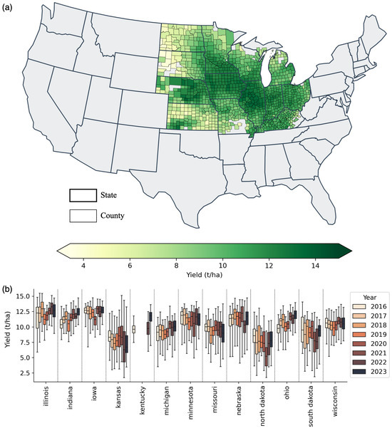
Figure 1.
The average corn yield map of Corn Belt for years between 2016 and 2023 (a) and boxplots showing county-level corn yield distributions (t/ha) by state and year (b).
2.2. Cropland Data Layer and Yield Statistics
The USDA [32] conducts a thorough annual assessment of crop productivity in the Corn Belt and produces a high-resolution crop type map, Cropland Data Layer (CDL). This study collected corn classification maps from 13 states at the county level and their corresponding yearly corn production information. Although the original yield statistics were acquired in bushels per acre (bu/acre), they were converted to tons per hectare (t/ha) for consistency. The data have a 30 m spatial resolution and are obtained from the Google Earth Engine (GEE) platform, which is freely available.
The average corn yield for each county was calculated during the years 2016–2023 together with the interannual and county-level corn yield variability per state, as presented in Figure 1. The USDA NASS database performs extensive data collection and releases this information freely to users, allowing the development of yield prediction models to encourage sustainable and manageable agriculture production. The yield data used in this study was obtained from https://quickstats.nass.usda.gov/ (accessed on 7 April 2025).
2.3. Earth Observation Datasets
The combination of satellite remote sensing data, climatic factors, and soil texture along with topography information enables the development of a robust yield prediction framework. Remote sensing data provide comprehensive information on crop health and phenological state through the analysis of the leaf area index (LAI), EVI, and land surface temperature (LST) in both the temporal and spatial domains. Climatic factors such as temperature and precipitation are indicative of the environmental influences essential for crop monitoring during the growing season. Topographic information and soil texture significantly influence micro-climatic conditions as well as soil holding capacity in terms of water and nutrients [33]. An overview of the features used in the crop yield prediction can be found in Table 1.

Table 1.
Detailed descriptions and spatial and temporal resolutions of the data used in this research.
2.3.1. Satellite Data
MODIS is a remote sensing satellite sensor on NASA’s Terra and Aqua satellites, providing global data on Earth’s surface, ocean, and atmosphere at moderate spatial resolution, widely used for environmental and agricultural monitoring. MODIS data are an incomparable source for extracting vegetation indices and biophysical parameters, providing vital insights into crop health, growth, and productivity, thus serving as a significant resource for extensive crop monitoring and yield prediction. The enhanced vegetation index (EVI) serves as information source regarding the crop health and greenness of vegetation, whereas normalized difference water index (NDWI) reflects the water content in both crops and soil. LAI provides metrics for crop density and photosynthetic activity, which are essential for evaluating phenological development. Land surface temperature (LST) indicates surface temperature fluctuations, crucial for understanding heat stress and evapotranspiration dynamics. These factors jointly improve the ability to observe and model agricultural production variations under diverse conditions in the Corn Belt. The EVI, NDWI, LAI, and LST were derived from MODIS data via the GEE platform.
2.3.2. Soil Texture
Soil texture, defined by the relative amounts of sand, silt, and clay, is an important factor in yield prediction, influencing retaining water, drainage, nutrient availability, and root development. Incorporating soil texture into yield prediction models improves understanding of its impact on soil moisture dynamics and nutrient cycles, which is critical to assessing crop phenology in various fields. This study uses soil texture data obtained from the SoilGrids collection via the GEE platform [34]. This dataset provides soil information at a spatial resolution of 250 m across several depth levels.
2.3.3. Topographic Data
Elevation (H) and slope (S) are critical topographic factors that influence crop yield prediction through affecting micro-climatic conditions and the spatial distribution of soil moisture. Integrating these variables into yield prediction models improves the model’s ability to provide a complete spectrum that considers spatial variability in agricultural production. The topographical variables were derived from SRTM-based DEM data [35] using the GEE platform. The dataset has a spatial resolution of 30 m globally.
2.3.4. Climate Data
The dynamics of crop phenology, a critically important part of the growing cycle, are significantly affected by climatic factors such as precipitation (P) and air temperature (T). This study obtained climate information from Daymet V4 [36] via the GEE platform. The Daymet V4 collection offers daily climatic factors with a spatial resolution of 1 km. We extracted precipitation in mm and minimum and maximum air temperatures in Celsius.
2.4. Data Exploratory Analysis and Preprocessing
The data undergo several preprocessing steps before being integrated with the yield data. This process includes aggregating satellite data, soil texture, topographic data, and climate data at the county level for the years 2016 to 2023. For this purpose, data are categorized into dynamic and static features. Dynamic features include time-varying variables such as climate and satellite data. These data cover precipitation, maximum and minimum temperatures, vegetation indices such as EVI, NDWI, and LAI, as well as daytime land surface temperature as examples of dynamic features. Static features, on the other hand, include attributes that remain constant or change over a long time. These include soil properties such as bulk density, sand, silt, and clay fractions, along with topographic characteristics like elevation and slope.
To prepare the data for analysis, the full time series was divided into eight periods, each spanning four weeks for which the dynamic features were aggregated. In this process, precipitation and surface temperature were calculated as a sum, while maximum and minimum temperatures, EVI, NDWI, and LAI were calculated as a mean. Missing values in dynamic features were interpolated to fill gaps. The time series is then smoothed using the Savitzky–Golay filter to reduce noise. As a final step, static and dynamic features were concatenated for each county. The statistics of these input features were presented in Table 2.
Table 2.
The general statistics of input features.
In order to understand the relationship between crop yield and input features, the variations in Pearson’s correlation coefficient were analyzed along the crop growing period on a 4-weekly basis (Figure 2). Most variables exhibited Pearson’s correlation coefficient exceeding approximately 0.3, indicating significant statistical relationships with crop yield. Satellite data demonstrated a stronger correlation with yield data compared to climate data. Among satellite variables, EVI (0.79), LST (0.55), and LAI (0.51) showed the highest correlations. The correlations were particularly strong during the period between August and October, with the exception of LST. Outside of this period, most of the satellite variables displayed negative correlations with yield. NDWI, which followed a pattern similar to LST, was negatively correlated with yield during the August to October period, while, outside this time frame, it exhibited a more positive correlation. For climate data, P and Tmax showed values with correlation coefficients ranging between 0.26 and 0.31.
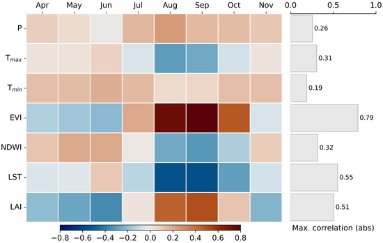
Figure 2.
Heatmap of Pearson correlation between dynamic features and crop yield along the phenology of corn. The right side of the figure shows the maximum correlation value through the phenology in an absolute manner.
3. Methods
The general overview of the workflow to build a county-level crop yield model for the time period 2016–2023 in the CONUS region using a spatio-temporal ML framework is shown in Figure 3. This process starts with creating a comprehensive EO dataset that is space–time overlayed with annual cropland maps to mask non-corn pixels and match with average yield statistics for each county where corn is planted. After preprocessing these layers, the combined dataset is used for both in-season and end-of-season yield prediction tasks to compare the performance of the KAN against the MLP, SVR, random forest regression (RFR), K-Nearest Neighbors (KNN), and Least Absolute Shrinkage and Selection Operator (LASSO) models. The models are validated using a leave-one-state-out cross-validation approach, with Bayesian hyperparameter optimization performed via the Optuna framework [37] to ensure they are properly trained. Finally, we produce county-level yield maps with their uncertainty estimates and explain how EO features impact the model predictions along the phenology of corn using the interpretability of KAN models.
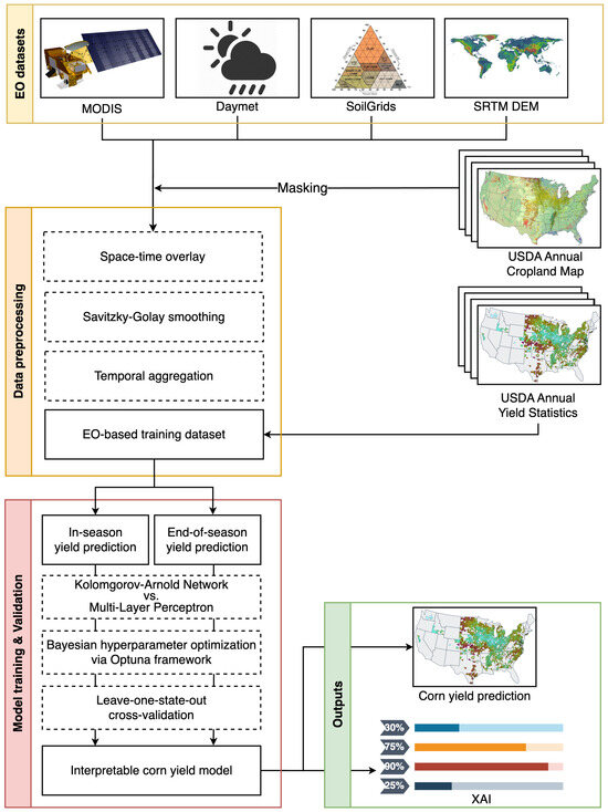
Figure 3.
Workflow for creating a space–time corn yield prediction model.
The methodology focuses primarily on the applicability of the KAN model to predict corn yield and its interpretability to analyze the driving force of corn production. As such, the study compares the performance of KAN with its main competitor, MLP, and also presents comparative results with well-known traditional ML algorithms to demonstrate its predictive accuracy performance. However, in this section, only the theoretical aspects of the MLP and KAN models are briefly explained. For detailed explanations of the other methods, please refer to [38].
3.1. Multi-Layer Perceptron
MLPs are the most widely known architecture of artificial neural networks [39]. They are the simplest examples of neural networks that feed forward and backward propagation. They are commonly used for classification and regression tasks in a variety of applications as they are relatively easy to train due to their simple architecture compared to more advanced DL models, yet they still have their ability to model complex relationships in datasets.
The structure of the MLP model starts with an input layer to which the input features are fed and ends with an output layer that performs prediction using a predefined activation function (see Figure 4). The model’s ability to comprehend highly nonlinear relations that exist between input and output is determined by the depth of the model and the number of neurons used in the layers. The depth of the model can be increased by adding intermediate layers, also called hidden layers, between the input and output layers, although this is not strictly necessary. The general formulation of MLP can be written as a weighted summation as follows:
where i represents the number of hidden layers, j represents the number of neurons in each hidden layer, is the bias vector, x is the input feature space with , and is the weight vector [40].
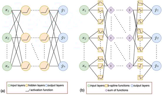
Figure 4.
Model architectures for (a) MLP and (b) KAN models.
3.2. Kolmogorov–Arnold Networks
KANs are based on the Kolmogorov–Arnold theorem [41], which claims that any multivariate continuous function can be represented by means of univariate functions and their summation. For a given multivariate function f, , it can be formulated as
where represents each variable that is contained between 0 and 1, i.e., for all n, and and are univariate functions. In this way, this relation suggests that the binary addition of the univariate functions ( and ) is sufficient to represent the multivariate function f in an exact manner [29].
KANs employ univariate spline functions, called learnable activation functions, which are updated iteratively during the training process as the model continues to learn (see Figure 4). This contrasts with the use of fixed activation functions such as ReLU or sigmoid in MLP. The univariate functions process each input feature independently, with their learned spline representations determining the unique contribution of each feature within the model. The splines, which are parameterized by trainable coefficients, establish the relationship between the input and the output. The univariate functions aggregate the summed outputs of , revealing how the characteristics interact to influence the predictions of the model. By visualizing the coefficient of the spline functions using their magnitude, we can derive an interpretable model. The shape and amplitude of the spline functions demonstrate the importance of individual features. This interpretability distinguishes the KAN model from MLP and enables a clear understanding of the contribution of features [29,41,42,43,44].
3.3. Implementation of Yield Estimation Framework
The input dataset contains eight time intervals between April and November of each year and 62 feature dimensions that consist of 56 dynamic and 6 static features. The value of a feature at each time step corresponds to the biweekly approximations along the phenology of corn, either averaged or summed (see Section 2.4 for details on the preprocessing of the data). The time steps of each dynamic feature were horizontally stacked, and, finally, all dynamic and static features were concatenated along the feature space, as illustrated in Figure 5. In this figure, each row represents the feature space of a county for a single year. There are nearly 6700 samples over six years for 13 states in the CONUS region. We split the data into 80% and 20% training and testing samples, respectively. During the fine-tuning of ML models, we adopted leave-one-state-out cross-validation framework to have generalized models across study area and to prevent models from overfitting. The final performance of the models was then objectively assessed on the basis of the testing dataset.
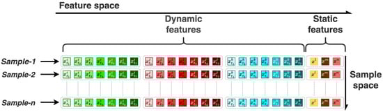
Figure 5.
A tabular representation of input data for KAN, and by extension other models.
3.4. Accuracy Assessment
We evaluated the numerical results of KAN and other ML models in corn yield prediction. The accuracy of the models was assessed using three accuracy metrics: coefficient of determination (R2), root mean square error (RMSE), and mean absolute error (MAE) to measure the accuracy of the predictions.
where n is the total number of counties used in the study, shows the actual value of the yield for the i-th county, represents the predicted yield value of the i-th county from the model, and corresponds to the mean of all yield values across all counties.
4. Results
This section presents the results of the corn yield prediction framework, beginning with model optimization through Bayesian hyperparameter tuning. This is followed by end-of-season model training and performance evaluation through comparison with other methods, accompanied by a feature importance analysis, and concluding with in-season corn yield forecasting.
4.1. Model Parameter Optimization
The hyperparameter tuning process is a crucial step in optimizing the performance of any ML or DL model as it ensures effective learning and generalization capability. To enable a fair comparison, we tuned the hyperparameters of each model to optimize their predictive performance and prevent possible overfit and underfit scenarios to fairly compare the accuracy of the models. We employed the Optuna framework [37], enabling us to efficiently test the hyperparameters in a given search space and determine optimal values for the model subject to tuning. Such a Bayesian optimization algorithm not only speeds up the tuning process but also leads to a more robust set of hyperparameters that maximize the model performance. Both MLP and the KAN have common key hyperparameters, including the number of hidden layers and unit size, which define model depth and neuron count, along with learning rate, activation function, optimizer, and regularization, which balance training stability and prevent overfitting. Additionally, the KAN introduces unique structural hyperparameters, such as grid size, which controls spline function parameterization, and entropy regularization, which encourages smoother functions and basis functions that determine the degree of the splines. In Table 3, the hyperparameter space tested and the optimized (i.e., selected) parameters for the MLP and KAN models are given.
Table 3.
Hyperparameter ranges and selected values for MLP and KAN models.
4.2. End-of-Season Yield Prediction
The overall performance comparison for all models is presented in Table 4. Among the models tested, the KAN showed the best predictive performance, achieving the highest R2 (0.85) and the lowest RMSE (0.84 t/ha). The RFR model performed relatively well, with an RMSE of 0.91 t/ha and an R2 value of 0.82, making it a strong candidate for such tasks despite its slightly higher error compared to KAN. On the other hand, the LASSO model produced the worst performance, demonstrating poor predictive capability, with the highest MAE (0.76 t/ha) and RMSE (1.01 t/ha). The KNN and MLP showed intermediate performance, with MAE and RMSE values higher than those of RFR and KAN, and R2 values of 0.81.
Table 4.
Performance metrics for different models. The units of MAE and RMSE are t/ha.
Figure 6 illustrates the regression plots for the corn yield estimations and the corresponding observed yield values. The KAN and RFR models show the tightest variation in observed vs. predicted values around the 1:1 line. The predictions tend to fall within 95% of the distribution (within the 2-standard deviation range). Obviously, these models can capture the relationship between input variables and corn yield more accurately than the other models, which supports the high R2 values given in Table 4. Although the LASSO method is quite effective in reducing overfitting due to its regularization properties, the model predictions show a wider spread outside the 95% confidence lines and a higher number of outliers. For the SVR model, the models noticeably overestimate the predictions in low-yield regions (<5 t/ha).
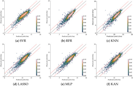
Figure 6.
Regression plots of observed and predicted corn yields for models: (a) SVM, (b) RFR, (c) KNN, (d) LASSO, (e) MLP, and (f) KAN. Black dashed lines are 1:1 lines, red dashed lines denote 95% distribution for residual values, and color bars represent the point density.
To associate which features play an important role during the phenology of corn in the Corn Belt, we visualized the feature attribution of the KAN model as a heatmap in Figure 7. It shows the normalized version of the importance of dynamic and static features for the corn yield prediction model in the CONUS. The dynamic features drive the model with a value of 88.3% in total importance, while the static features account for 11.7%. Among the dynamic features, the EVI is the most significant (25%), followed by (14%) and LAI (12%). The cumulative importance of the monthly features exceeds 70% three months before harvest, with August being the most important month (18% importance). The heatmap demonstrates that EVI and LAI, along with the climatic variable , are the most influential variables in the corn yield model.
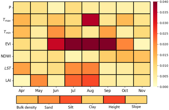
Figure 7.
The importance of features along the crop growth period.
4.3. In-Season Yield Prediction
Timely crop yield forecasting plays a critical role in agricultural management by enabling the early detection of potential production failures. This allows farmers to optimize resource allocation during key growth stages while providing policymakers and stakeholders with valuable data for market stabilization and food security planning.
In order to test how accurately the KAN can model corn yield before the harvest period, we trained yield forecasting models using only certain periods along the phenology. Starting in April, which represents the first time frame (t1), we trained seven in-season prediction models, each of which includes an additional month until the end-of-season (t8). In fact, the model we presented at t8 is the exact same model that we trained regarding the end-of-season prediction, making a total of eight prediction models.
Figure 8 shows the temporal change in the prediction performance of all the in-season yield models (from April to October) together with the end-of-season model, given in the above section. The regression plot of each in-season yield model during the growth period is illustrated in Figure 9. In the early season of the crop’s phenology, using only April (t1) and April–May (t1–t2), the model can explain only 58% of the variations in the yield (R2 = 0.58). With the inclusion of periods after May to the feature space, the model performance begins to improve noticeably. In the early-season stages, April to May, the forecast errors, both MAE and RMSE, are relatively high, with the maximum RMSE taking place in May. There is no apparent change in the R2 value at the beginning of the season. Moving toward the mid-season period, from June till August, the forecast errors significantly decline and the model begins to gain some predictive strength as time progresses. In August, the model’s performance reaches a level where it is almost as accurate as the end-of-season predictions. Towards the late season, from September to November, MAE and RMSE stabilize at lower values with minimal fluctuations. The R2 values do not show any noteworthy increase or decrease, which signals consistent predictive accuracy as the crop season concludes.
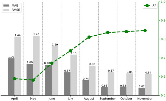
Figure 8.
In-season corn yield prediction via KAN model.
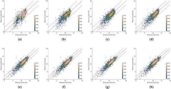
Figure 9.
Regression plots for in-season corn yield forecasting models from April to November for all years. Black dashed lines are 1:1 lines, red dashed lines denote 95% distribution for residual values, and color bars represent the point density. (a) Only April (t1). (b) April–May (t1–t2). (c) April–June (t1–t3). (d) April–July (t1–t4). (e) April–August (t1–t5). (f) April–September (t1–t6). (g) April–October (t1–t7). (h) April–November (t1–t8).
5. Discussion
Corn is a crucial staple food that can be qualified as a strategic product due to its critical role in various sectors, including its use as animal feed and industrial raw materials. In this context, the United States, one of the world’s largest producers, plays a pivotal role in meeting the demands of both domestic and international markets. However, in recent years, corn production in the U.S. has faced significant challenges arising from environmental factors and regional variability [45,46]. The first among these challenges is climate change, which has direct impacts on agricultural production, most notably reduced water availability, extreme climatic events, and decreased soil fertility [24,47,48,49]. Meanwhile, the rapid growth of the global population suggests a substantial increase in corn consumption and demand in different sectors [50]. This trend poses serious threats to food security and economic stability. To ensure sufficient food availability, it is essential to develop sustainable agricultural policies that are strengthened with emerging technologies [19,51]. In this sense, rather than relying on short-term solutions to increase corn production, efforts should focus on the effective management of agricultural land and production processes.
Based on the accuracy results obtained in Table 4, the KAN model demonstrated high predictive accuracy for corn yield, outperforming the MLP and other ML models tested. It consistently achieved lower RMSE and MAE values and the highest R2, which is also implied in the scatter plots of the observed and predicted corn yields for all models (see Figure 6). These results suggest that a KAN is more effective in capturing complex nonlinear relationships between EO features derived from satellite observations and county-based corn yield statistics. Notably, the end-of-season prediction accuracy of the KAN model is similar to that in other county-level corn yield prediction studies across the U.S. Corn Belt. For example, a study conducted by Khan et al. [7] reported R2 values of 0.861, 0.856, and 0.854 using partial least squares linear regression, SVR, and ridge regression methods, respectively. Similarly, Mateo-Sanchis et al. [19] found the accuracy of regularized linear regression and kernel ridge regression models as ∼0.90 using one year of county-level data.
Beyond accuracy, the KAN’s architecture allowed us to gather insights into the drivers of corn yield. The importance of features throughout the growing season, visualized in Figure 7, aligns well with the typical stages of corn growth. The key features influencing yield prediction provide clear evidence at particular periods, supporting corn development’s phenological timeline. During the period from June to September, the importance of the EVI is at its highest, which aligns closely with the peak of corn’s vegetative growth and reproductive stages. This is the period in which the crop canopy is fully developed and performing photosynthetic activities, making the EVI a vital indicator for assessing crop health by monitoring its greenness and understanding variations in yield. During the same period, in July and August, the LAI is also quite effective in the predictive performance of the model, followed by a significantly high impact of the daily maximum temperature in August and LST in July and August. These results of temporal feature importance agree well with the study conducted by Ma et al. [52], although they did not perform a temporal analysis. For the prediction of corn yield, they found that EVI and LAI were the most important features after historical yield information. The LST and values were also found to be effective in their analysis, confirming the relationship between optimal temperature and photosynthetic activity. Our findings are consistent with the study conducted by Mateo-Sanchis et al. [23] that used a shallow LSTM model to predict the county-level corn yield values in the same study area between 2015 and 2018. They also highlighted the dominant influence of EVI and values, with their peak during the summer season between June and August. It is worth noting that the KAN model offers a direct and explicit interpretation of feature importance compared to the post hoc explanation techniques, integrated gradients, and Shapley additive explanations implemented in Mateo-Sanchis et al. [23].
Furthermore, we present the in-season corn yield forecast results to evaluate the predictive accuracy of the model during the growing season. From the beginning of the growing season to harvesting, there is a clear increase in model performance. One of the standout features of any operational crop yield model is its ability to accurately forecast crop yield early in the growing season. Of course, the question that must be answered would be how early the KAN-based crop yield model can forecast the potential yield outcome that will be harvested at the end of the crop season. In an attempt to answer this question, we designed an experiment where we gradually increased the temporal period bimonthly along the corn phenology and observed the change in the model’s performance in terms of R2 and forecast errors. The model achieved reasonable accuracy even at the vegetative stage, where inputs such as early-season weather and soil conditions dominated. As expected, the model performance was lower in these early months compared to end-of-season accuracy. During the period from sowing until the plant completes its vegetative stage, which lasts approximately until the end of June, the model’s value remains below 0.7. As seen in Figure 2, the correlation between the features used in the model and the yield data is also very low during this time period [13,52]. By mid-season, as more phenological data became available, the forecasts improved significantly and reached a level competitive with the late-season predictions. Once the plant completes its vegetative stage and reaches its maximum greenness, starting from July, the model performance exceeds 0.7. In August, which corresponds to the period in which corn transitions from the vegetative stage to the reproductive stage, the model value exceeds 0.80, reaching a performance level very close to the end-of-season value (). This enables high-accuracy yield predictions approximately three months before harvest. Ma et al. [52] compared the end-of-season performance of a Bayesian neural network model with its in-season performance, similarly observing that the model reached an value of 0.8 in August, converging to the end-of-season value.
The performance of the KAN can be attributed to its use of learnable spline functions, which offer a flexible alternative to the fixed activations used in traditional MLPs. This enables the KAN to dynamically adjust its activation patterns to the complex nonlinear correlations present in EO data of agricultural land, which are affected by the interaction of climate, soil, and management variables. Moreover, the KAN’s architecture fundamentally enhances interpretability and adaptability in function representation. Using this approach, the spatially and temporally varied responses of corn yields to environmental and climatic factors are better captured across corn fields throughout the CONUS, in contrast to models with fixed functional forms. However, it remains important to explore how the KAN expands and generalizes to larger datasets, different geographical regions, and agroclimatic conditions. Thus, testing the transferability of the KAN to other regions or possibly other crop types is necessary to prove its scalability, similar to the methodology employed by Khan et al. [24].
6. Conclusions
In this study, we implemented a state-of-the-art KAN architecture to obtain an interpretable crop yield model that integrates satellite remote sensing data with climate, topography, and soil parameters to predict the corn yield in the CONUS Corn Belt. According to the numerical results, the KAN-based corn yield estimation model demonstrated better performance comparison results regarding six regression models, including the KAN itself. The findings clearly demonstrate the need for advanced architectures such as the KAN in agricultural decision-making, particularly to address the complex relationships inherent in EO signals and crop yield, as well as to explain how these characteristics impact crop yield along the phenological cycle.
In addition to end-of-season yield prediction, we performed in-season corn yield forecasting to demonstrate how early the KAN model can capture the dynamics of biophysical and geophysical properties along crop growth with reasonable accuracy, enabling it to serve as an operational model in agricultural planning. The KAN model can forecast the observed yield with a coefficient of determination greater than 0.8 approximately three months before harvest, which is significantly close to the accuracy achieved regarding the end-of-season yield prediction (R2 = 0.85). Moreover, the interpretable nature of the model architecture helps us to investigate which features contribute the most to the model prediction by analyzing the weights estimated by the spline functions. According to the results, the most influential factor is the EVI, in particular during the peak of the growing season from June to August, followed by the LAI, again in the same period. The most influential climate variable is maximum value of air temperature. Our findings demonstrate that the KAN model can effectively predict county-level corn yields and provide interpretable insights into its predictions. This indicates that the model successfully reflects the intricate dynamics within crop production systems. In future work, we will investigate how KAN-based corn yield prediction models trained in the Corn Belt can be generalized to other regions around the world with different climatological and pedological conditions using transfer learning approaches.
Author Contributions
Conceptualization, M.S.I., O.O. and M.F.C.; methodology, M.F.C.; software, M.S.I. and M.F.C.; validation, O.O. and M.F.C.; formal analysis, M.S.I., O.O. and M.F.C.; investigation, O.O.; resources, M.S.I., O.O. and M.F.C.; data curation, M.F.C.; writing—original draft preparation, M.S.I., O.O. and M.F.C.; writing—review and editing, M.S.I., O.O. and M.F.C.; visualization, M.S.I. All authors have read and agreed to the published version of the manuscript.
Funding
The first author was supported by the European Union’s Horizon Europe research and innovation programme through the Open-Earth-Monitor Cyberinfrastructure project under grant agreement No. 101059548.
Data Availability Statement
All the Earth Observation datasets used in this study are available from the Google Earth Engine (GEE) data catalog at https://developers.google.com/earth-engine/datasets (accessed on 7 April 2025).
Acknowledgments
The authors would like to acknowledge USDA for corn yield statistics. The Python 3 implementation of the Kolmogorov–Arnold Network trained in this work can be accessed through https://github.com/KindXiaoming/pykan (accessed on 7 April 2025). The hyperparameter tuning of the models was carried out using the Optuna 4.4 framework (https://github.com/optuna/optuna) (accessed on 7 April 2025).
Conflicts of Interest
The authors declare no conflicts of interest.
Abbreviations
The following abbreviations are used in this manuscript:
| CDL | Crop Data Layer |
| CONUS | Continental United States |
| DEM | Digital Elevation Model |
| DL | Deep Learning |
| EO | Earth Observation |
| EVI | Enhanced Vegetation Index |
| GEE | Google Earth Engine |
| H | Height |
| KANs | Kolmogorov–Arnold Networks |
| KNN | K-Nearest Neighbors |
| LAI | Leaf Area Index |
| LASSO | Least Absolute Shrinkage and Selection Operator |
| LST | Land Surface Temperature |
| LSTM | Long Short-Term Memory |
| MAE | Mean Absolute Error |
| ML | Machine Learning |
| MLP | Multi-Layer Perceptron |
| MODIS | Moderate-Resolution Imaging Spectroradiometer |
| NDWI | Normalized Difference Water Index |
| P | Precipitation |
| RFR | Random Forest Regression |
| RMSE | Root Mean Square Error |
| S | Slope |
| SRTM | Shuttle Radar Topography Mission |
| SVR | Support Vector Regression |
| U.S. | United States |
| XAI | Explainable Artificial Intelligence |
References
- Kopittke, P.M.; Menzies, N.W.; Wang, P.; McKenna, B.A.; Lombi, E. Soil and the intensification of agriculture for global food security. Environ. Int. 2019, 132, 105078. [Google Scholar] [CrossRef] [PubMed]
- Yuan, X.; Li, S.; Chen, J.; Yu, H.; Yang, T.; Wang, C.; Huang, S.; Chen, H.; Ao, X. Impacts of Global Climate Change on Agricultural Production: A Comprehensive Review. Agronomy 2024, 14, 1360. [Google Scholar] [CrossRef]
- Rosegrant, M.W.; Cline, S.A. Global Food Security: Challenges and Policies. Science 2003, 302, 1917–1919. [Google Scholar] [CrossRef] [PubMed]
- Meroni, M.; Waldner, F.; Seguini, L.; Kerdiles, H.; Rembold, F. Yield forecasting with machine learning and small data: What gains for grains? Agric. For. Meteorol. 2021, 308–309, 108555. [Google Scholar] [CrossRef]
- Luo, Y.; Zhang, Z.; Cao, J.; Zhang, L.; Zhang, J.; Han, J.; Zhuang, H.; Cheng, F.; Tao, F. Accurately mapping global wheat production system using deep learning algorithms. Int. J. Appl. Earth Obs. Geoinf. 2022, 110, 102823. [Google Scholar] [CrossRef]
- Zhou, W.; Liu, Y.; Ata-Ul-Karim, S.T.; Ge, Q.; Li, X.; Xiao, J. Integrating climate and satellite remote sensing data for predicting county-level wheat yield in China using machine learning methods. Int. J. Appl. Earth Obs. Geoinf. 2022, 111, 102861. [Google Scholar] [CrossRef]
- Khan, S.N.; Khan, A.N.; Tariq, A.; Lu, L.; Malik, N.A.; Umair, M.; Hatamleh, W.A.; Zawaideh, F.H. County-level corn yield prediction using supervised machine learning. Eur. J. Remote Sens. 2023, 56, 2253985. [Google Scholar] [CrossRef]
- Lu, J.; Fu, H.; Tang, X.; Liu, Z.; Huang, J.; Zou, W.; Chen, H.; Sun, Y.; Ning, X.; Li, J. GOA-optimized deep learning for soybean yield estimation using multi-source remote sensing data. Sci. Rep. 2024, 14, 7097. [Google Scholar] [CrossRef] [PubMed]
- Muruganantham, P.; Wibowo, S.; Grandhi, S.; Samrat, N.H.; Islam, N. A Systematic Literature Review on Crop Yield Prediction with Deep Learning and Remote Sensing. Remote Sens. 2022, 14, 1990. [Google Scholar] [CrossRef]
- Cao, J.; Zhang, Z.; Tao, F.; Zhang, L.; Luo, Y.; Han, J.; Li, Z. Identifying the Contributions of Multi-Source Data for Winter Wheat Yield Prediction in China. Remote Sens. 2020, 12, 750. [Google Scholar] [CrossRef]
- Peng, B.; Guan, K.; Pan, M.; Li, Y. Benefits of Seasonal Climate Prediction and Satellite Data for Forecasting U.S. Maize Yield. Geophys. Res. Lett. 2018, 45, 9662–9671. [Google Scholar] [CrossRef]
- Timsina, J.; Humphreys, E. Performance of CERES-Rice and CERES-Wheat models in rice–wheat systems: A review. Agric. Syst. 2006, 90, 5–31. [Google Scholar] [CrossRef]
- Johnson, D.M. An assessment of pre- and within-season remotely sensed variables for forecasting corn and soybean yields in the United States. Remote Sens. Environ. 2014, 141, 116–128. [Google Scholar] [CrossRef]
- Khaki, S.; Wang, L. Crop Yield Prediction Using Deep Neural Networks. Front. Plant Sci. 2019, 10, 621. [Google Scholar] [CrossRef] [PubMed]
- Peichl, M.; Thober, S.; Samaniego, L.; Hansjürgens, B.; Marx, A. Machine-learning methods to assess the effects of a non-linear damage spectrum taking into account soil moisture on winter wheat yields in Germany. Hydrol. Earth Syst. Sci. 2021, 25, 6523–6545. [Google Scholar] [CrossRef]
- Khan, S.N.; Li, D.; Maimaitijiang, M. A Geographically Weighted Random Forest Approach to Predict Corn Yield in the US Corn Belt. Remote Sens. 2022, 14, 2843. [Google Scholar] [CrossRef]
- Ebrahimy, H.; Wang, Y.; Zhang, Z. Utilization of synthetic minority oversampling technique for improving potato yield prediction using remote sensing data and machine learning algorithms with small sample size of yield data. ISPRS J. Photogramm. Remote Sens. 2023, 201, 12–25. [Google Scholar] [CrossRef]
- Celik, M.F.; Isik, M.S.; Taskin, G.; Erten, E.; Camps-Valls, G. Explainable Artificial Intelligence for Cotton Yield Prediction with Multisource Data. IEEE Geosci. Remote Sens. Lett. 2023, 20, 8500905. [Google Scholar] [CrossRef]
- Mateo-Sanchis, A.; Piles, M.; Muñoz-Marí, J.; Adsuara, J.E.; Pérez-Suay, A.; Camps-Valls, G. Synergistic integration of optical and microwave satellite data for crop yield estimation. Remote Sens. Environ. 2019, 234, 111460. [Google Scholar] [CrossRef] [PubMed]
- Martinez-Ferrer, L.; Piles, M.; Camps-Valls, G. Crop Yield Estimation and Interpretability with Gaussian Processes. IEEE Geosci. Remote Sens. Lett. 2021, 18, 2043–2047. [Google Scholar] [CrossRef]
- Jhajharia, K.; Mathur, P. Prediction of crop yield using satellite vegetation indices combined with machine learning approaches. Adv. Space Res. 2023, 72, 3998–4007. [Google Scholar] [CrossRef]
- Li, Y.; Zeng, H.; Zhang, M.; Wu, B.; Zhao, Y.; Yao, X.; Cheng, T.; Qin, X.; Wu, F. A county-level soybean yield prediction framework coupled with XGBoost and multidimensional feature engineering. Int. J. Appl. Earth Obs. Geoinf. 2023, 118, 103269. [Google Scholar] [CrossRef]
- Mateo-Sanchis, A.; Adsuara, J.E.; Piles, M.; Munoz-Marí, J.; Perez-Suay, A.; Camps-Valls, G. Interpretable Long Short-Term Memory Networks for Crop Yield Estimation. IEEE Geosci. Remote Sens. Lett. 2023, 20, 2501105. [Google Scholar] [CrossRef]
- Khan, S.N.; Li, D.; Maimaitijiang, M. Using gross primary production data and deep transfer learning for crop yield prediction in the US Corn Belt. Int. J. Appl. Earth Obs. Geoinf. 2024, 131, 103965. [Google Scholar] [CrossRef]
- Terliksiz, A.S.; Altilar, D.T. Impact of large kernel size on yield prediction: A case study of corn yield prediction with SEDLA in the U.S. Corn Belt. Environ. Res. Commun. 2024, 6, 025011. [Google Scholar] [CrossRef]
- Sakamoto, T. Incorporating environmental variables into a MODIS-based crop yield estimation method for United States corn and soybeans through the use of a random forest regression algorithm. ISPRS J. Photogramm. Remote Sens. 2020, 160, 208–228. [Google Scholar] [CrossRef]
- Sartore, L.; Rosales, A.N.; Johnson, D.M.; Spiegelman, C.H. Assessing machine leaning algorithms on crop yield forecasts using functional covariates derived from remotely sensed data. Comput. Electron. Agric. 2022, 194, 106704. [Google Scholar] [CrossRef]
- Paudel, D.; de Wit, A.; Boogaard, H.; Marcos, D.; Osinga, S.; Athanasiadis, I.N. Interpretability of deep learning models for crop yield forecasting. Comput. Electron. Agric. 2023, 206, 107663. [Google Scholar] [CrossRef]
- Liu, Z.; Wang, Y.; Vaidya, S.; Ruehle, F.; Halverson, J.; Soljačić, M.; Hou, T.Y.; Tegmark, M. KAN: Kolmogorov-Arnold Networks. arXiv 2024, arXiv:2404.19756. [Google Scholar] [PubMed]
- Teymoor Seydi, S.; Sadegh, M.; Chanussot, J. Kolmogorov–Arnold Network for Hyperspectral Change Detection. IEEE Trans. Geosci. Remote Sens. 2025, 63, 5505515. [Google Scholar] [CrossRef]
- Jamali, A.; Roy, S.K.; Hong, D.; Lu, B.; Ghamisi, P. How to Learn More? Exploring Kolmogorov–Arnold Networks for Hyperspectral Image Classification. Remote Sens. 2024, 16, 4015. [Google Scholar] [CrossRef]
- USDA. United States Department of Agriculture National Agricultural Statistics Service. Available online: https://quickstats.nass.usda.gov/ (accessed on 12 January 2023).
- Celik, M.F.; Isik, M.S.; Yuzugullu, O.; Fajraoui, N.; Erten, E. Soil Moisture Prediction from Remote Sensing Images Coupled with Climate, Soil Texture and Topography via Deep Learning. Remote Sens. 2022, 14, 5584. [Google Scholar] [CrossRef]
- Poggio, L.; de Sousa, L.M.; Batjes, N.H.; Heuvelink, G.B.M.; Kempen, B.; Ribeiro, E.; Rossiter, D. SoilGrids 2.0: Producing soil information for the globe with quantified spatial uncertainty. Soil 2021, 7, 217–240. [Google Scholar] [CrossRef]
- Jarvis, A.; Reuter, H.I.; Nelson, A.; Guevara, E. Hole-Filled SRTM for the Globe Version 4. CGIAR-CSI SRTM 90m Database. 2008. Available online: https://research.utwente.nl/en/publications/hole-filled-srtm-for-the-globe-version-4-data-grid (accessed on 7 April 2025).
- Thornton, M.; Shrestha, R.; Wei, Y.; Thornton, P.; Kao, S.C. Daymet: Daily Surface Weather Data on a 1-km Grid for North America, Version 4. 2020. Available online: https://daac.ornl.gov/cgi-bin/dsviewer.pl?ds_id=1840 (accessed on 7 April 2025).
- Akiba, T.; Sano, S.; Yanase, T.; Ohta, T.; Koyama, M. Optuna: A Next-generation Hyperparameter Optimization Framework. In Proceedings of the 25rd ACM SIGKDD International Conference on Knowledge Discovery and Data Mining, Anchorage, AK, USA, 4–8 August 2019. [Google Scholar]
- Raschka, S.; Mirjalili, V. Python MachineLearning: Machine Learning and Deep Learning with Python, Scikit-Learn, and TensorFlow 2; Packt Publishing Ltd.: Birmingham, UK, 2019. [Google Scholar]
- Murtagh, F. Multilayer perceptrons for classification and regression. Neurocomputing 1991, 2, 183–197. [Google Scholar] [CrossRef]
- Haykin, S. Neural Networks and Learning Machines, 3/E; Pearson Education: Tamil Nadu, India, 2009. [Google Scholar]
- Vaca-Rubio, C.J.; Blanco, L.; Pereira, R.; Caus, M. Kolmogorov-Arnold Networks (KANs) for Time Series Analysis. arxiv 2024, arXiv:2405.08790. [Google Scholar]
- Liu, Z.; Ma, P.; Wang, Y.; Matusik, W.; Tegmark, M. Kan 2.0: Kolmogorov-arnold networks meet science. arXiv 2024, arXiv:2408.10205. [Google Scholar]
- Genet, R.; Inzirillo, H. TKAN: Temporal Kolmogorov-Arnold Networks. arxiv 2024, arXiv:2405.07344. [Google Scholar] [CrossRef]
- Xu, K.; Chen, L.; Wang, S. Kolmogorov-Arnold Networks for Time Series: Bridging Predictive Power and Interpretability. arxiv 2024, arXiv:2406.02496. [Google Scholar]
- Sun, J.; Lai, Z.; Di, L.; Sun, Z.; Tao, J.; Shen, Y. Multilevel Deep Learning Network for County-Level Corn Yield Estimation in the U.S. Corn Belt. IEEE J. Sel. Top. Appl. Earth Obs. Remote Sens. 2020, 13, 5048–5060. [Google Scholar] [CrossRef]
- Pede, T.; Mountrakis, G.; Shaw, S.B. Improving corn yield prediction across the US Corn Belt by replacing air temperature with daily MODIS land surface temperature. Agric. For. Meteorol. 2019, 276–277, 107615. [Google Scholar] [CrossRef]
- Huang, H.; Huang, J.; Feng, Q.; Liu, J.; Li, X.; Wang, X.; Niu, Q. Developing a Dual-Stream Deep-Learning Neural Network Model for Improving County-Level Winter Wheat Yield Estimates in China. Remote Sens. 2022, 14, 5280. [Google Scholar] [CrossRef]
- Lischeid, G.; Webber, H.; Sommer, M.; Nendel, C.; Ewert, F. Machine learning in crop yield modelling: A powerful tool, but no surrogate for science. Agric. For. Meteorol. 2022, 312, 108698. [Google Scholar] [CrossRef]
- Teng, J.; Hou, R.; Dungait, J.A.J.; Zhou, G.; Kuzyakov, Y.; Zhang, J.; Tian, J.; Cui, Z.; Zhang, F.; Delgado-Baquerizo, M. Conservation agriculture improves soil health and sustains crop yields after long-term warming. Nat. Commun. 2024, 15, 8785. [Google Scholar] [CrossRef] [PubMed]
- Qiao, M.; He, X.; Cheng, X.; Li, P.; Luo, H.; Zhang, L.; Tian, Z. Crop yield prediction from multi-spectral, multi-temporal remotely sensed imagery using recurrent 3D convolutional neural networks. Int. J. Appl. Earth Obs. Geoinf. 2021, 102, 102436. [Google Scholar] [CrossRef]
- Kira, O.; Wen, J.; Han, J.; McDonald, A.J.; Barrett, C.B.; Ortiz-Bobea, A.; Liu, Y.; You, L.; Mueller, N.D.; Sun, Y. A scalable crop yield estimation framework based on remote sensing of solar-induced chlorophyll fluorescence (SIF). Environ. Res. Lett. 2024, 19, 044071. [Google Scholar] [CrossRef]
- Ma, Y.; Zhang, Z.; Kang, Y.; Özdoğan, M. Corn yield prediction and uncertainty analysis based on remotely sensed variables using a Bayesian neural network approach. Remote Sens. Environ. 2021, 259, 112408. [Google Scholar] [CrossRef]
Disclaimer/Publisher’s Note: The statements, opinions and data contained in all publications are solely those of the individual author(s) and contributor(s) and not of MDPI and/or the editor(s). MDPI and/or the editor(s) disclaim responsibility for any injury to people or property resulting from any ideas, methods, instructions or products referred to in the content. |
© 2025 by the authors. Licensee MDPI, Basel, Switzerland. This article is an open access article distributed under the terms and conditions of the Creative Commons Attribution (CC BY) license (https://creativecommons.org/licenses/by/4.0/).