Spatial and Spectral Structure-Aware Mamba Network for Hyperspectral Image Classification

Abstract

Recently, a network based on selective state space models (SSMs), Mamba, has emerged as a research focus in hyperspectral image (HSI) classification due to its linear computational complexity and strong long-range dependency modeling capability. Originally designed for 1D causal sequence modeling, Mamba is challenging for HSI tasks that require simultaneous awareness of spatial and spectral structures. Current Mamba-based HSI classification methods typically convert spatial structures into 1D sequences and employ various scanning patterns to capture spatial dependencies. However, these approaches inevitably disrupt spatial structures, leading to ineffective modeling of complex spatial relationships and increased computational costs due to elongated scanning paths. Moreover, the lack of neighborhood spectral information utilization fails to mitigate the impact of spatial variability on classification performance. To address these limitations, we propose a novel model, Dual-Aware Discriminative Fusion Mamba (DADFMamba), which is simultaneously aware of spatial-spectral structures and adaptively integrates discriminative features. Specifically, we design a Spatial-Structure-Aware Fusion Module (SSAFM) to directly establish spatial neighborhood connectivity in the state space, preserving structural integrity. Then, we introduce a Spectral-Neighbor-Group Fusion Module (SNGFM). It enhances target spectral features by leveraging neighborhood spectral information before partitioning them into multiple spectral groups to explore relations across these groups. Finally, we introduce a Feature Fusion Discriminator (FFD) to discriminate the importance of spatial and spectral features, enabling adaptive feature fusion. Extensive experiments on four benchmark HSI datasets demonstrate that DADFMamba outperforms state-of-the-art deep learning models in classification accuracy while maintaining low computational costs and parameter efficiency. Notably, it achieves superior performance with only 30 training samples per class, highlighting its data efficiency. Our study reveals the great potential of Mamba in HSI classification and provides valuable insights for future research.

1. Introduction

1.1. Background

In the field of remote sensing, hyperspectral imaging and synthetic aperture radar [1,2] have attracted widespread attention from researchers. With the development of hyperspectral imaging technology, the acquisition of hyperspectral images (HSIs) has become increasingly convenient and efficient [3]. Unlike ordinary visual images that only have RGB channels, HSIs capture the spatial information of the target object while also capturing dozens or even hundreds of continuous spectra. Benefiting from this rich and detailed spectral information, HSIs enable more precise object identification through comprehensive characterization of material composition, structural properties, and physical states. Owing to these advantages, HSIs are widely used in various fields, such as medical imaging [4,5], agriculture [6], mineral resource exploration [7], and so on. HSI classification, as a key link in these applications, has always been a research hotspot.

HSI classification methods are generally categorized into traditional machine learning (ML) and deep learning (DL) methods. In early research, numerous ML-based methods were successfully applied to HSI classification, including support vector machines (SVMs) [8], logistic regression [9], random forests [10], and k-means clustering [11]. With the advancement of deep learning techniques, HSI classification has witnessed remarkable progress in recent years. Current mainstream DL architectures can be roughly divided into convolutional neural networks (CNNs) [12,13,14], graph convolutional networks (GCNs) [15,16], and Transformers [17]. HSI datasets acquired by optical sensors (e.g., AVIRIS, ROSIS, ITRES CASI 1500) encounter several notable challenges in land cover classification: (1) the high dimensionality of spectral data, which leads to the curse of dimensionality and redundant information; (2) spatial variability, where pixels of the same class exhibit distinct spectral responses due to varying illumination, background mixing, or environmental conditions; and (3) the scarcity of labeled samples, as pixel-level annotation in remote sensing is expensive and time-consuming. These challenges demand models that can efficiently capture both spectral and spatial dependencies while remaining robust under limited supervision. To address the above challenges, deep learning methods such as CNNs and Transformer have been widely applied to hyperspectral image classification. CNNs are effective at modeling local spatial structures but are inherently limited by their receptive fields, making it difficult to capture long-range spatial dependencies. Transformer-based methods, on the other hand, can model global contextual relationships, but they typically require large-scale labeled datasets and involve high computational complexity, which limits their applicability in low-sample settings. These inherent limitations of existing models hinder further improvements in HSI classification accuracy, highlighting the need for an efficient approach that can capture long-range spatial dependencies while maintaining relatively low computational complexity.

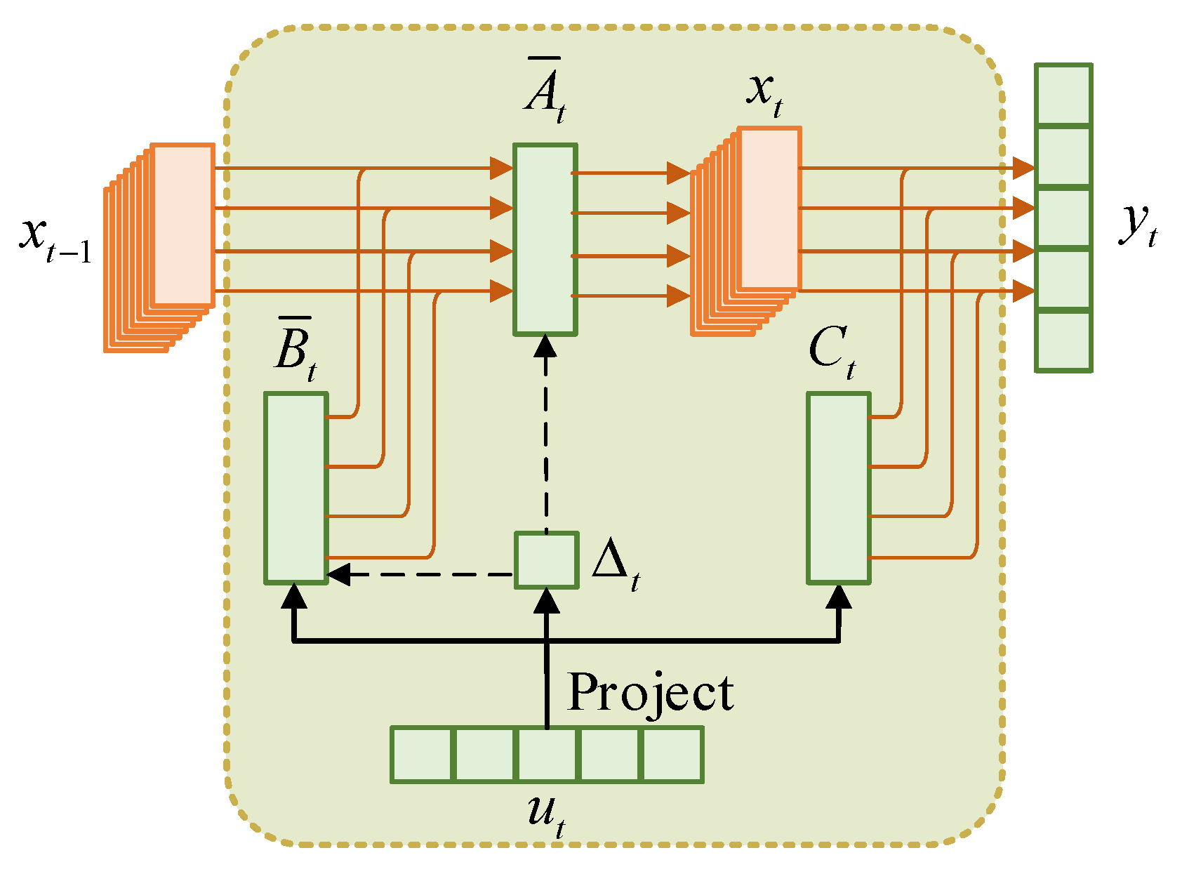
Recently, state-space models (SSMs) [18] have aroused heated discussions in the field of DL; especially structured state-space sequence models (S4) [19] have attracted widespread attention in sequence modeling. Mamba [20] introduced a selection mechanism based on S4, enabling the model to selectively retain input-dependent information while maintaining indefinite memory. By employing a hardware-aware algorithm, Mamba achieves higher computational efficiency than Transformer. Benefiting from its linear complexity in modeling long-range dependencies, Mamba has achieved remarkable success in language modeling [20]. Inspired by the success of Mamba in language modeling, more and more Mamba-based methods have been applied to the field of HSI classification [21,22,23]. However, due to the image-spectrum merging characteristic of HSI, existing Mamba-based HSI classification methods still have the following limitations. On the one hand, unlike 1D sequences, the HSI spatial dimension is a 2D spatial structure. Current Mamba-based HSI classification methods [24,25,26,27] typically flatten the 2D spatial structure into the 1D sequence and then use a fixed scanning strategy to extract spatial features from the 1D sequence, which inevitably changes the spatial relationship between pixels, destroys the inherent contextual information in the image, and affects the classification results. On the other hand, current Mamba-based HSI classification methods [21,25] usually extract spectral features from the perspective of changing the spectral scanning direction, without considering the dependency of neighboring spectral information. In addition, these strategies of adding scanning directions inevitably increase the computational cost. These limitations compel us to design a structure-aware HSI classification model capable of capturing both spatial and spectral dependencies between neighboring features in the latent state space.

1.2. Related Work

HSI classification methods in early research primarily focused on spectral feature extraction from HSIs. Traditional approaches such as principal component analysis (PCA) [28,29], independent component analysis (ICA) [30], and linear discriminant analysis (LDA) [31] were commonly employed for HSI classification. However, these conventional methods exhibited limited generalization capability and weak representational capacity for the extracted features, resulting in unsatisfactory classification performance. In contrast, DL techniques not only demonstrate superior generalization ability but can also adaptively learn high-level semantic features. These advantages have led to their widespread application across various research domains, particularly in image classification [32,33,34], object detection [35,36,37,38], and semantic segmentation [39].

Among the prevalent backbone networks in DL, CNNs and their variants have been widely adopted for HSI classification. This is because they can effectively extract high-level semantic features and conveniently capture both spectral and spatial characteristics of HSIs. Hu et al. [40] treated spectral information as objects and employed 1D-CNN to extract spectral-dimensional features for HSI classification. To incorporate spatial information, Makantasis et al. [41] first reduced HSI dimensionality through R-PCA, then used patches of neighboring pixels around central pixels as training samples for 2D-CNN-based classification. However, using 2D-CNN alone cannot simultaneously capture joint spectral-spatial features. Hamida et al. [42] segmented HSIs into 3D cubes suitable for 3D-CNN processing, stacking multiple 3D-CNN layers for classification. Roy et al. [43] proposed a HybridSN network, combining 2D-CNN and 3D-CNN strategies, where 3D-CNN first extracted joint spectral-spatial features, followed by 2D-CNN learning more abstract spatial features. As network depth increases, models may encounter the gradient vanishing issue during training. To address this, He et al. [44] introduced residual connections. Zhong et al. [45] developed an end-to-end spectral-spatial residual network (SSRN) that complements feature information between each 3D convolutional layer and subsequent layers through residual blocks, achieving cross-layer feature enhancement and significantly improving classification performance. Zhang et al. [46] proposed a CNN-based spectral partitioning residual network (SPRN) that divides input spectra into multiple sub-bands and employs parallel improved residual blocks for feature extraction, effectively enhancing spectral-spatial feature representation. However, these CNN-based methods are fundamentally limited by their kernel sizes, resulting in insufficient understanding of global HSI structures. Furthermore, CNNs cannot establish long-range dependencies, making them ineffective for comprehensive spectral information extraction.

In recent years, Transformers have emerged as another mainstream framework for HSI classification due to their powerful long-range modeling capability and global spatial feature extraction ability. Dosovitskiy et al. [47] pioneered the Vision Transformer (ViT), marking a significant attempt to apply Transformer in the visual domain by directly processing sequences of image patches. Subsequently, numerous ViT variants have been adapted for HSI classification. Hong et al. [48] proposed a pure Transformer-based network named SpectralFormer for sequential information extraction in HSI classification. However, SpectralFormer underutilizes spatial positional information, resulting in suboptimal classification performance. To address this limitation, Sun et al. [49] developed an SSFTT network, which first converts shallow spectral-spatial features extracted by convolutional layers into deep semantic tokens, then employs Transformer for semantic modeling. This CNN–Transformer hybrid architecture effectively captures high-level semantic features to improve classification accuracy. Roy et al. [50] introduced a novel model named MorphFormer that integrates learnable spectral and spatial morphological convolutions with Transformer to enhance interactions between image tokens and class tokens regarding structural and shape information in HSI. Ma et al. [51] proposed LSGA-ViT, incorporating a light self-Gaussian-attention (LSGA) mechanism with Gaussian absolute position bias to better simulate HSI data distribution, making attention weights more concentrated around central query patches. Zhao et al. [52] observed that the inherent global correlation modeling in Transformer overlooks effective representation of local spatial-spectral features. To address this, they developed GSC-ViT, which specifically enhances the extraction of local spectral-spatial information. However, the self-attention mechanism [17] presents computational challenges due to its quadratic complexity, which not only increases computational costs but also limits the model’s capacity for long-range dependency modeling [53].

Recently, a new DL architecture, SSMs, has attracted widespread attention in the academic community. SSMs are good at capturing long-range dependencies and can be efficiently parallelized [53], positioning them as a strong competitor to CNNs and Transformers. Mamba is a typical representative of SSMs, with excellent computational efficiency and powerful feature extraction capability. In computer vision, Zhu et al. [53] designed a general vision backbone network named Vision Mamba (Vim) based on the location sensitivity of visual data and the global context requirements of visual understanding. The network uses a bidirectional Mamba structure to replace the self-attention mechanism. Liu et al. [54] proposed a VMamba network, which introduced the Cross-Scan Module (CSM) to traverse the spatial domain and transform any non-causal visual image sequence patch sequence, which helps to narrow the gap between the orderliness of one-dimensional selective scanning and the non-sequential structure of 2D visual data. In the field of remote sensing, Chen et al. [55] proposed an RSMamba for remote sensing image classification. The model proposed a dynamic multi-path activation mechanism to enhance Mamba’s ability to model non-causal data. Cao et al. [56] proposed a model called M3amba, a new end-to-end CLIP-driven Mamba model for multimodal fusion, and designed a multimodal Mamba fusion architecture with linear complexity and a cross-attention module Cross-SS 2D for full and effective information fusion. In HSI classification, Sun et al. [26] proposed a DBMamba model, which first used CNN to extract shallow spectral spatial features and then used bidirectional Mamba to extract higher-level semantic features based on the shallow features to achieve classification. Huang et al. [23] proposed an SS-Mamba model, which first converts the HSI cube to spatial and spectral token sequences through a token generation module. The sequences processed by Mamba blocks are then fed into a feature enhancement module for final classification. Lu et al. [57] developed the SSUM model, comprising the Spectral Mamba branch and the Spatial Mamba branch, where the features output from both branches are combined to produce classification results. Wang et al. [25] proposed an LE-Mamba model for HSI classification, using a multi-directional local spatial scanning mechanism in the spatial dimension to improve the extraction of non-causal local features and a bidirectional scanning mechanism in the spectral dimension to capture fine spectral details. He et al. [22] proposed a new 3DSS-Mamba framework. In order to overcome the limitations of the traditional Mamba algorithm that can only model causal sequences and is not suitable for high-dimensional scenes, an algorithm based on the 3D-Spectral-Spatial Selective Scanning (3DSS) mechanism was proposed, and five scanning paths were constructed to examine the impact of dimensional priority [22]. Existing Mamba-based HSI classification methods attempt to solve the problem of aligning HSI spatial structure with sequential Mamba by continuously adjusting the scanning strategy, but there are limitations in effectiveness and efficiency. In addition, when processing HSI spectral information, only considering the spectral scanning direction cannot fully extract the intrinsic information of the spectrum.

1.3. Motivation and Contribution

HSI classification is to classify each pixel into a certain category, and a single pixel shows a certain correlation with its spatially close pixels. Making full use of spatial structural information is conducive to improving the classification results. Conventional classification methods use image patches centered on classified pixels as the input of the model. However, Mamba-based models usually convert 2D image patches into 1D sequences for spatial feature scanning. Although existing scanning strategies partially solve the problem of insufficient feature extraction after the spatial structure is converted into a sequence structure, they have certain limitations in terms of effectiveness and efficiency. On the one hand, directional scanning inevitably changes the spatial relationship between pixels, thereby destroying the original semantic information. For example, the distance between a pixel and its left or right (horizontal) neighbor is 1, while the distance between its upper or lower (vertical) neighbor is equal to the width of the 2D image patch, which hinders the model from understanding the spatial relationship in the original HSI 2D image patch. On the other hand, fixed scanning paths [24,25,26,27], such as four-directional scanning [25], cannot effectively capture the complex spatial relationship in the 2D image patch, and the introduction of more scanning directions requires additional calculations. In addition, HSI has spatial variability [58]; that is, pixels of the same category present different spectral features in space, which increases the difficulty of the model in extracting spectral features and thus affects the overall classification performance.

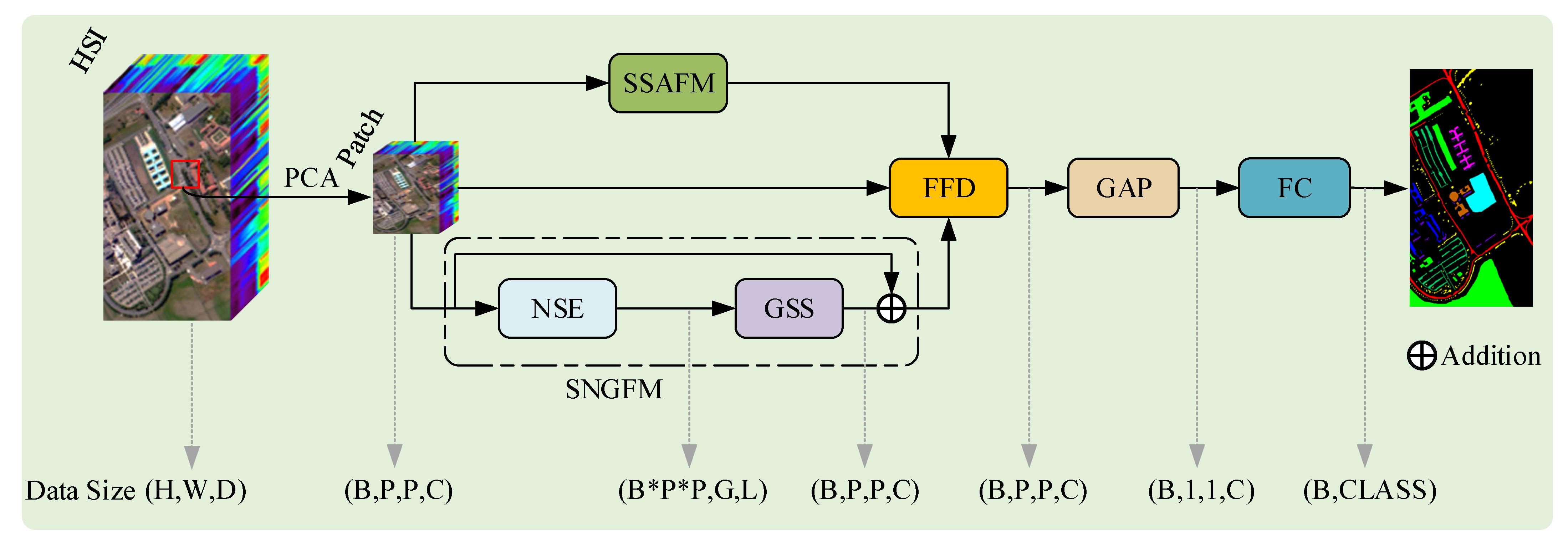
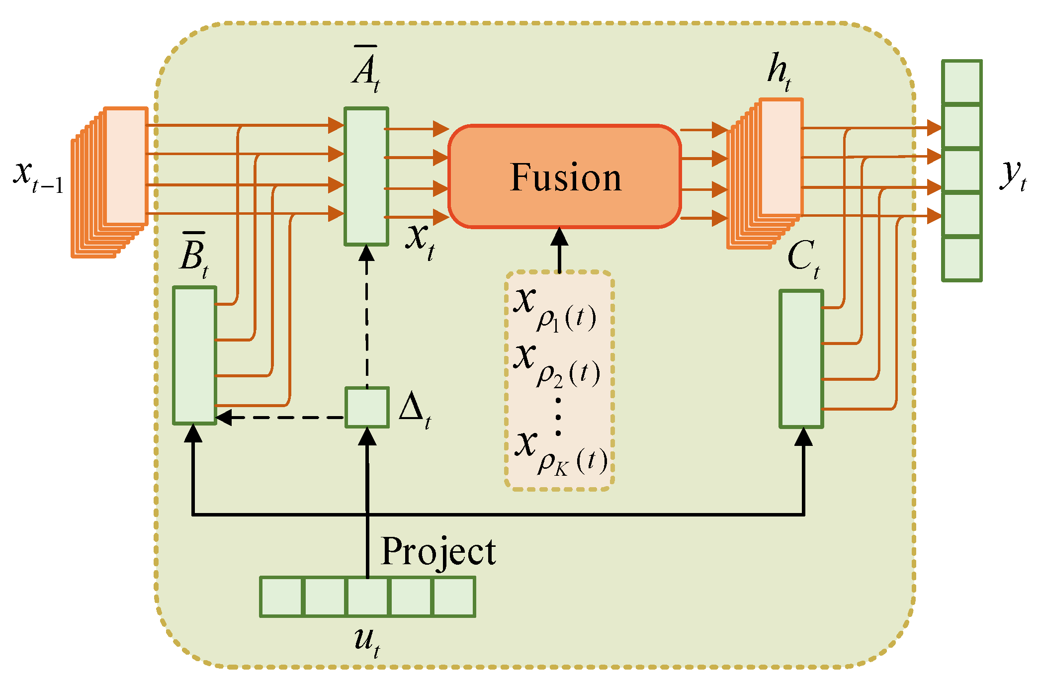
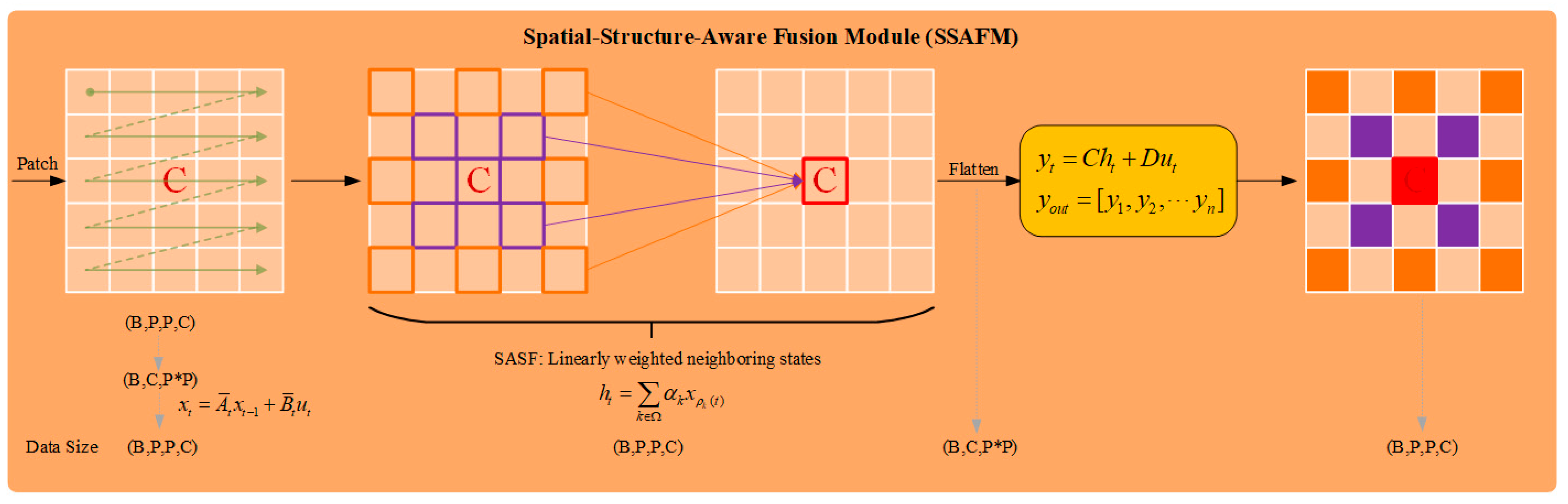
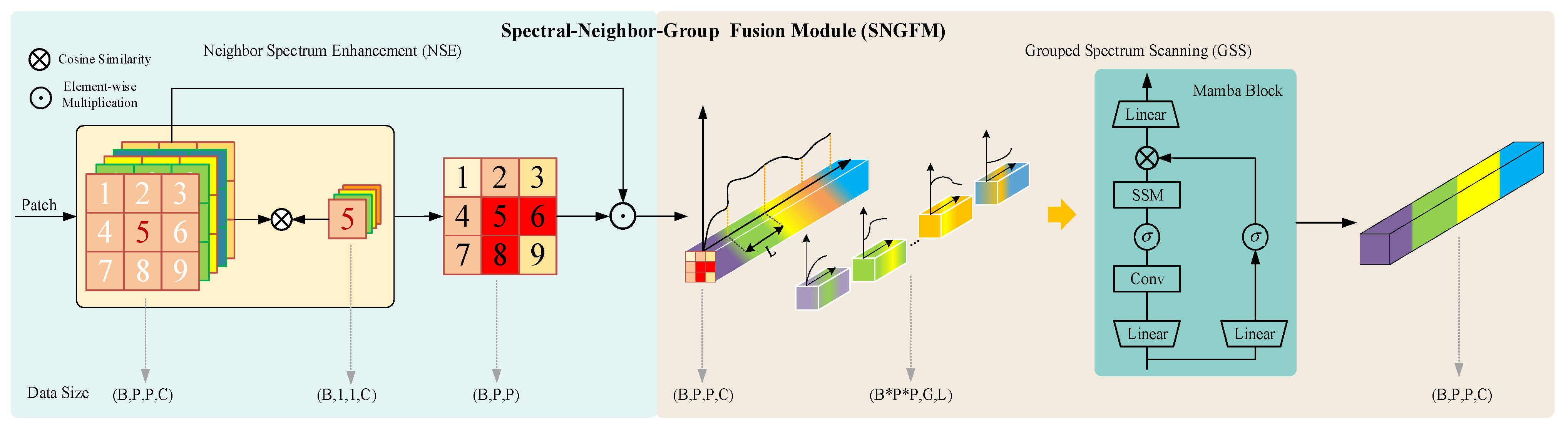
In order to overcome the limitations of existing scanning strategies and mitigate the impact of spatial variability, this paper proposes a new HSI classification framework named Dual-Aware Discriminative Fusion Mamba (DADFMamba). DADFMamba not only captures the spatial dependency of HSI neighboring features from the latent state space, but also uses the spectral features of the target pixel’s neighbors to reduce spatial variability, thereby improving the classification performance. DADFMamba consists of the Spatial-Structure-Aware Fusion Module (SSAFM), the Spectral-Neighbor-Group Fusion Module (SNGFM) and the Feature Fusion Discriminator (FFD). In SSAFM, a new structure-aware state fusion (SASF) equation is introduced into the original Mamba to effectively capture the HSI spatial features. In SNGFM, a neighbor spectrum enhancement (NSE) strategy is proposed to overcome the interference caused by spatial variability. On this basis, a new scanning mechanism, grouped spectrum scanning (GSS), is proposed, which divides the enhanced spectral features into several small groups to better distinguish the subtle differences in spectral information. At the same time, this mechanism makes the model computationally friendly. Finally, FFD with a residual structure is used to implement HSI classification.

The main contributions of this paper are summarized as follows:

• A new Mamba-based HSI classification method named Dual-Aware Discriminative Fusion Mamba (DADFMamba) is proposed. It achieves dual awareness of HSI spatial and spectral structures by modeling spatial structure context and spectral neighborhood correlation in a unified framework.
• In SSAFM, to address the challenge of spatial structure loss in existing Mamba-based HSI classification methods, we introduce a novel structure-aware state fusion (SASF) equation. This equation not only enables effective skip connections between non-sequential elements in the sequence but also enhances the model’s ability to capture spatial relationships in HSIs.
• In SNGFM, in order to overcome the interference caused by spatial variability, a new NSE strategy is proposed. In addition, in order to better distinguish the subtle differences in spectral features, a new GSS mechanism is developed. Through the organic combination of the two, both the spectral feature extraction capability and computational efficiency are improved.

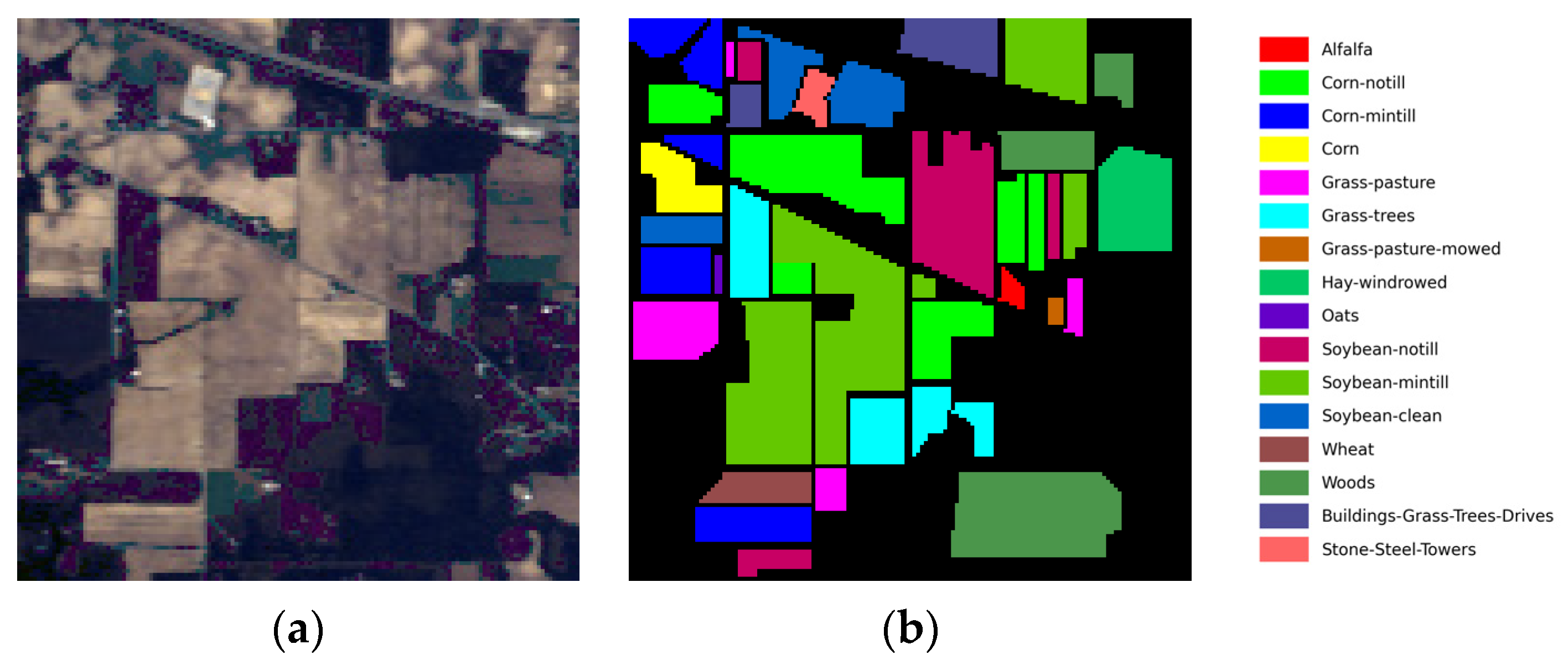
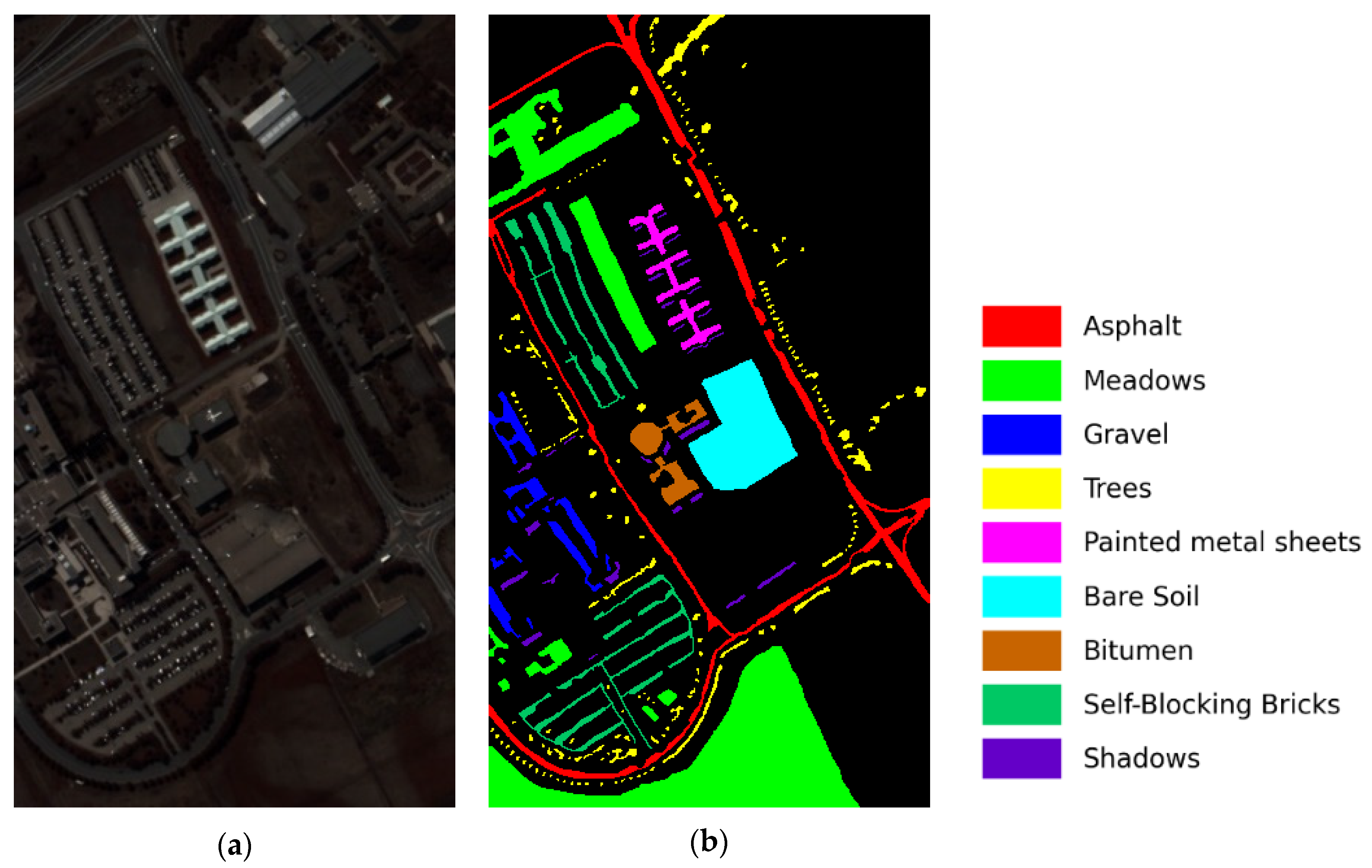
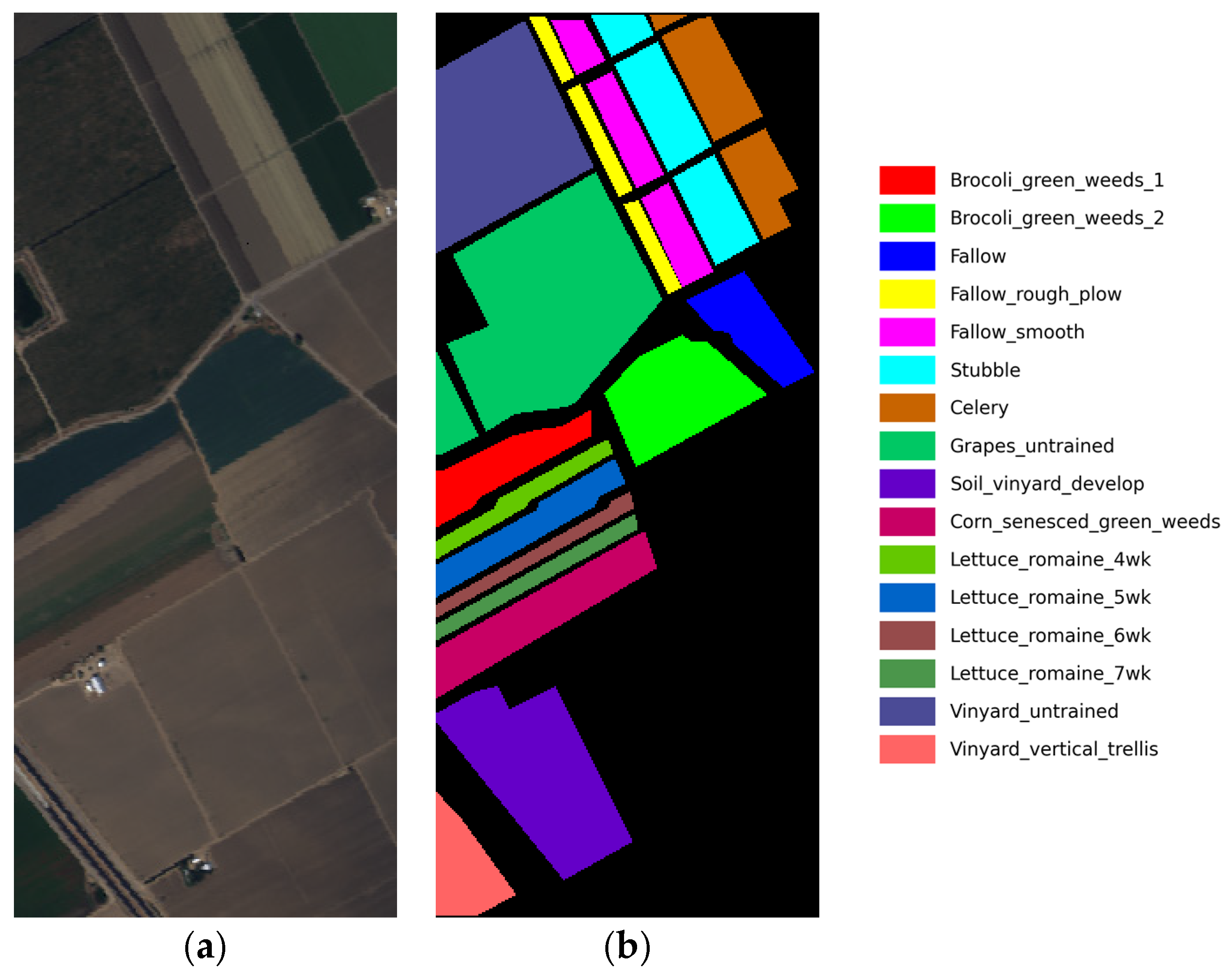
The remainder of this paper is organized as follows. Section 2 introduces the State Space Model and presents the detailed architecture of the proposed DADFMamba. Section 3 comprehensively describes the experimental process, including dataset selection, implementation details, comparative experiments, parameter analysis, and ablation studies. Finally, Section 4 concludes this work and provides suggestions for future research directions.

2. Material and Methods

2.1. Preliminaries

Recently, structured state space models (S4) have been actively influenced by RNNs, CNNs and the classic state space model and have shown great potential in sequence modeling. Equations (1)–(3) follow the classical Kalman filter formulation for linear dynamical systems, originally proposed in [59], and later introduced into the deep learning context by Mamba [20]. A one-dimensional function or sequence $u(t)\in ℝ$ is used as input, and the output is mapped to $y(t)\in ℝ$, $u(t)\in ℝ\mapsto y(t)\in ℝ$, through a state variable $x(t)\in {ℝ}^N$. This process can be expressed by the linear ordinary differential Equation (1), using $A\in {ℝ}^{\mathrm{N}\times \mathrm{N}}$ as the state transfer matrix, $B\in {ℝ}^{\mathrm{N}}$ and $C\in {ℝ}^{\mathrm{N}}$ as the projection parameters, and $D$ implemented using skip connections.

$$\begin{array}{c}{x}^{\prime }(t)=Ax(t)+Bu(t),\\ y(t)=Cx(t)+Du(t).\end{array}.$$

(1)

In order to effectively extend the continuous system to DL to process discrete problems such as images and natural language, the continuous system needs to be discretized. Usually the zero-order hold (ZOH) rule is used for discretization, and the time scale parameter $\Delta$ is introduced to represent the interval between discrete time steps, and the continuous parameters $A$ and $B$ are transformed into discrete parameters $\overline{A}$ and $\overline{B}$. This can be obtained by Formula (2).

$$\begin{array}{l}\overline{A}=\exp (\Delta A),\\ \overline{B}={(\Delta A)}^{-1}(\exp (\Delta A)-I)\cdot \Delta B.\end{array}.$$

(2)

Although traditional state space models (SSMs) have achieved linear time complexity, since they are time-invariant systems, parameters $\Delta$, $B$, and $C$ cannot be flexibly adjusted according to the changes in data at different time steps, resulting in an inability to accurately describe processes that change over time in the real world. To overcome this limitation, Mamba improves SSM through a selection mechanism to make the model parameters input-dependent and change with different inputs, thus turning it into a time-varying system. This can pay more attention to relevant information and provide a more accurate and realistic representation of dynamic systems. Specifically, by modifying parameters $\Delta$, $B$, and $C$ to simple functions of the input sequence $u(t)$, input-dependent parameters ${\Delta }_t=s_{\Delta }(u_t)$, $B_t=s_B(u_t)$, and $C_t=s_C(u_t)$ are obtained. Then the input-dependent discrete parameters ${\overline{A}}_t$ and ${\overline{B}}_t$ are calculated accordingly. The discrete state transition and observation equations can be obtained from Equation (3).

$$\begin{array}{l}{x}_t={\overline{A}}_t{x}_{t-1}+{\overline{B}}_t{u}_t,\\ y_t=C_t{x}_t+D{u}_t.\end{array}.$$

(3)

The process described above can be briefly summarized in Figure 1.

2.2. Overview

This paper proposes a Dual-Aware Discriminative Fusion Mamba (DADFMamba) model, which is specifically designed to capture the spatial correlation of neighboring pixel features in HSI and discriminate the spectral details in HSI. The overall architecture is shown in Figure 2 and can be divided into three key components: Spatial-Structure-Aware Fusion Module (SSAFM), Spectral-Neighbor-Group Fusion Module (SNGFM), and Feature Fusion Discriminator (FFD).

Specifically, the original HSI data $X\in {ℝ}^{H\times W\times D}$, where $H$, $W$ and $D$ represent the height, width and number of spectral channels, respectively, and the label corresponding to each pixel is $Y_i\in \left\{1,2,3,\dots ,\mathrm{Class}\right\}$. In order to retain the main spectral information and remove redundant information, principal component analysis (PCA) dimensionality reduction is first performed to obtain $X_{pca}\in {ℝ}^{H\times W\times C}$, where $C$ represents the reduced spectral dimension. For the patch-level-based HSI classification method, in order to avoid the loss of edge information, after edge filling of $X$, 3D patches are extracted on the data $X_{pca}$ to obtain 3D patch $I\in {ℝ}^{P\times P\times C}$, where $P$ is the size of the patch. Finally, the processed data are randomly divided into training and test sets and input into the model.

Spatial autocorrelation is a fundamental property in geographic information science and remote sensing, rooted in the principle of spatial proximity, namely, spatially adjacent units tend to exhibit higher similarity [60]. In HSI, this phenomenon is particularly prominent, as neighboring pixels typically belong to the same land-cover class and present similar spectral responses. Inspired by this observation, leveraging both spatial structural information and spectral characteristics from neighboring pixels can significantly enhance the classifier’s discriminative capability for the center pixel. To this end, we propose an SSAFM and an NSE strategy, which aim to improve feature representation by modeling local spatial structures and reinforcing spectral consistency. These designs contribute to improved classification accuracy and robustness in HSI classification tasks. In the proposed model, the SSAFM is first introduced to maximally utilize HSI spatial neighborhood information during feature extraction. This module directly establishes connectivity between neighboring HSI pixels in the state space by applying linear weighting to neighboring state variables within each neighborhood, thereby extracting features that incorporate HSI spatial structures. This operation enhances the model’s sensitivity to land-cover boundaries and spatial adjacency relationships. Concurrently, the SNGFM incorporates spectral information from neighboring pixels to augment the target pixel’s spectral characteristics. The enhanced features are then partitioned into small-range patches to extract intrinsic physical properties of land-cover categories, effectively reducing the impact of spatial variability on classification results. Subsequently, the FFD serves as a discriminator to assess the relative importance of spatial and spectral features. It adaptively assigns weights to the spatial features from SSAFM and spectral features from SNGFM, enabling optimal spatial-spectral feature fusion. The fused feature maps then undergo a Global Average Pooling (GAP) operation, reducing their spatial dimensions to 1 × 1. Finally, the pooled features are flattened into a 1D vector and fed into a fully connected classifier to produce the final classification results.

2.3. Spatial-Structure-Aware Fusion Module (SSAFM)

In order to make full use of spatial structural information for HSI classification, image patches centered on the classified pixels are conventionally used as input. However, the Mamba model typically converts 2D image patches into 1D sequence data and performs various scanning strategies on the 1D sequence data. This will destroy the original spatial structure of HSI and affect the classification results. In order to solve this problem and maintain the spatial structural relationship between pixels in HSIs, SSAFM is proposed. Different from the existing methods of scanning HSI from multiple directions [24,25,26], this module introduces a new structure-aware state fusion (SASF) equation to the original Mamba, which can be described by Equation (4). The spatial dependency of neighboring features of HSI is captured from the latent state space.

$$\begin{array}{l}{x}_t={\overline{A}}_t{x}_{t-1}+{\overline{B}}_t{u}_t,\\ h_t={\displaystyle \sum _{k\in \Omega }{\alpha }_k{x}_{{\rho }_k(t)}},\\ y_t=C_t{h}_t+D{u}_t.\end{array},$$

(4)

where $x_t$ is the original state variable, $h_t$ is the structure-aware state variable, $\Omega$ is the neighbor set, and ${\rho }_k(t)$ is the index of the kth neighbor of position $t$. Figure 3 illustrates the SSM flow in SSAFM. Compared with the original Mamba in Figure 1, it can be seen that the original state variable $x_t$ is directly affected by its previous state $x_{t-1}$, while the structure-aware state variable $h_t$ combines the additional neighboring state variables $x_{{\rho }_1(t)},x_{{\rho }_2(t)},\cdots ,x_{{\rho }_K(t)}$ through a fusion mechanism, where $K=|\Omega |$ represents the size of the neighbor set. By considering spatial and temporal information, the fused variable $h_t$ obtains richer semantics, thereby improving adaptability and a more comprehensive understanding of HSI.

The details of the SSAFM are shown in Figure 4. The HSI data $I\in {ℝ}^{P\times P\times C}$ of the input model is first flattened from the spatial dimension to a 1D sequence $u_t$ and the state $x_t$ is calculated using the state transition equation $x_t={\overline{A}}_t{x}_{t-1}+{\overline{B}}_t{u}_t$. The calculated state is reshaped into a 2D format. In order to enable each state to perceive its neighboring states in the 2D space, the SASF equation $h_t={\displaystyle \sum _{k\in \Omega }{\alpha }_k{x}_{{\rho }_k(t)}}$ is introduced. For the state variable $x_t$, the weight ${\alpha }_k$ is used to apply linear weighting to the neighboring states ${\rho }_k(t)$ in its neighborhood set $\Omega$, effectively integrating the local dependency information into the new state $h_t$, reducing the dependence on a single state information, thereby improving the prediction performance of the overall context. Finally, the output is obtained from $h_t$ through the observation equation $y_t=C_t{h}_t+D{u}_t$. The process can be described by Equation (5).

$$\begin{array}{cc}\hfill I_{flatten}& \in {ℝ}^{S\times C}=Flatten(I\in {ℝ}^{P\times P\times C}),\hfill \\ \hfill I_{reshaped}& \in {ℝ}^{P\times P\times C}=Reshape(Transition(I_{flatten}\in {ℝ}^{S\times C})),\hfill \\ \hfill I_{SF}& \in {ℝ}^{S\times C}=Flatten(SASF(I_{reshaped}\in {ℝ}^{P\times P\times C})),\hfill \\ \hfill I_{spa}& \in {ℝ}^{P\times P\times C}=Reshape(Observation(I_{SF}\in {ℝ}^{S\times C})).\hfill \end{array},$$

(5)

where $P$ and $C$ represent the spatial dimension size and number of channels of the input model data patch, respectively. Flatten and Reshape refer to flattening and reshaping into a visual format in the spatial dimension, respectively, resulting in $S=P\times P$. Transition and Observation represent the state transition equation and observation equation, respectively. The SASF equation can not only capture the local features of the image but also retain the global context modeling ability of the original Mamba model to a certain extent, thereby achieving a more comprehensive visual representation.

In practice, three 3 × 3 depth-wise kernels with dilation factors d = 1, 3, and 5 are used to construct the HSI feature neighbor set ${\Omega }_d=\{(i,j)|i,j\in \{-d,0,d\}\}$, and the SASF equation can be rewritten as Equation (6).

$$h_t={\displaystyle \sum _{d=1,3,5}{\displaystyle \sum _{i,j\in {\Omega }_d}{k}_{ij}^d\cdot x_{t+iP+j}}},$$

(6)

where $k_{ij}^d$ represents the kernel weight of the dilation factor d at position $(i,j)$, $x_{t+iw+j}$ represents the neighbor of state $x_t$ at position $(i,j)$, and $P$ represents the width of the HSI patch.

2.4. Spectral-Neighbor-Group Fusion Module (SNGFM)

In addition to spatial structural information, HSIs also carry a large amount of spectral information. Reasonable use of spectral information can complement spatial information and improve the model’s ability to distinguish fine-grained information. The existing Mamba-based methods [25,26] directly use Mamba or Mamba with a bidirectional scanning mechanism to process the entire spectral data and do not use the spectral information of the target pixel’s spatial neighborhood. Since HSI has spatial variability, this will affect the model’s ability to identify substances. In addition, the spectral information of HSI contains a lot of redundant information, which will greatly increase the computational cost. Based on the above considerations, we designed SNGFM. First, the spectral information of the spatial neighborhood is used to enhance the spectral features of the target pixel. Then, in order to reduce data redundancy in HSI and facilitate the SSM to focus on subtle differences in the spectral domain, the enhanced spectral features are partitioned into groups, enabling efficient spectral information extraction through grouped scanning, as shown in Figure 5.

2.4.1. Neighbor Spectrum Enhancement (NSE)

In order to alleviate the phenomenon that the same substance exhibits different spectral characteristics due to spatial variability, it is very important to use neighboring spectrum information to enhance the spectral characteristics of the target pixel. The patch $I\in {ℝ}^{P\times P\times C}$ obtained after PCA dimensionality reduction is input into the module, where $P$ and $C$ are the size of the patch and the dimension of the spectrum after PCA dimensionality reduction, respectively. Cosine similarity [61] is widely used to measure the angular similarity between high-dimensional vectors. In the context of HSI, each pixel can be viewed as a high-dimensional spectral vector. By computing the cosine similarity between a target pixel and its neighboring pixels, the method effectively captures spectral consistency, which is crucial for preserving material identity across spatial regions. This similarity measure is scale-invariant, ensuring robustness to illumination variation, a common challenge in real-world HSI acquisition. Moreover, this mechanism can be interpreted under the framework of graph signal processing, where each pixel is a node and similarity-based edge weights reflect the strength of connections. The enhanced feature representation thus approximates a spectral-aware spatial smoothing process that improves intra-class compactness and inter-class separability in the learned feature space. Considering that the information of the classified pixel plays a dominant role in the patch, the cosine similarity $s(g_{i,j}\cdot g_c)$ between the classified pixel and the spectral information of each spatial neighborhood pixel in the patch is calculated to obtain the similarity weight $Q$. The more similar the two are, the more likely they are to obtain a higher score, while the score of the noise pixel is lower. Then the input $I\in {ℝ}^{P\times P\times C}$ patch and $Q$ are weighted to obtain the spectral feature $I{E}_{spe}\in {ℝ}^{P\times P\times C}$ of the classified pixel enhancement. The whole processing process is shown in the following formula:

$$s(g_{i,j}\cdot g_c)={\displaystyle \frac{g_{i,j}^T\cdot g_c}{||g_{i,j}||\cdot ||g_c||}},$$

(7)

$$Q_{i,j}={\displaystyle \frac{s(g_{i,j}\cdot g_c)}{\max (s(g_{i,j}))-\min (s(g_{i,j}))}},$$

(8)

$$I{E}_{spe}=I\odot Q,$$

(9)

where $\odot$ is the element-wise multiplication operation and $i,j$ is the coordinate of the pixel in the patch.

2.4.2. Grouped Spectrum Scanning (GSS)

The inherent redundancy in HSIs presents significant challenges for efficient feature extraction. To address this issue, the proposed grouped scanning method effectively mitigates spectral redundancy by partitioning spectral bands into multiple fixed-length subgroups and processing each independently using selective state space models. This decomposition transforms high-dimensional spectral data into multiple low-dimensional subproblems, which not only enhances the model’s capacity to discern subtle spectral variations but also makes the framework more computationally friendly.

Specifically, the enhanced spectral feature $I{E}_{spe}\in {ℝ}^{P\times P\times C}$ is divided into G groups of length L $I{G}_{spe}\in {ℝ}^{P\times P\times G\times L}$ from the spectral dimension and scanned using Mamba, where $P$ and $C$ are the size of the patch and the dimension of the spectrum after PCA dimensionality reduction, $L=C/G$, and C is set to be exactly divisible by G. The extracted spectral feature $I_{spe}\in {ℝ}^{P\times P\times C}$ can be obtained by the following formula:

$$I{G}_{spe}=SplitGroup(I{E}_{spe}),$$

(10)

$$I{F}_{spe}=Flatten(I{G}_{spe}),$$

(11)

$$I{R}_{spe}=SiLU(GN(Mamba(I{F}_{spe}))),$$

(12)

$$I_{spe}=Reshape(I{R}_{spe})+I{E}_{spe},$$

(13)

where $I{R}_{spe}\in {ℝ}^{P^2\times G\times L}$ represents the features extracted by Mamba, G denotes the number of groups, and L indicates the length of each group.

2.5. Feature Fusion Discriminator (FFD)

In this paper, SSAFM and SNGFM extract the spatial and spectral features of HSI, respectively. SSAFM captures neighborhood spatial features from the state space, and SNGFM extracts spectral features in groups after introducing neighborhood spectral information. To effectively integrate spectral and spatial features for classification, we adopt a commonly used weighted feature fusion strategy, similar to that in [62]. Specifically, we introduce a Feature Fusion Discriminator (FFD) module, which adaptively evaluates the contribution of spatial and spectral features to the classification outcome and guides the feature fusion by assigning appropriate weights. Furthermore, considering the demand for sample-efficient models in HSI classification, we incorporate residual learning to mitigate potential overfitting during training. The fusion process can be formally expressed as follows:

$$I_{fus}=I+{\omega }_{spa}\cdot I_{spa}+{\omega }_{spe}\cdot I_{spe},$$

(14)

where $I_{fus}\in {ℝ}^{P\times P\times C}$ denotes the fused spatial-spectral features, while ${\omega }_{spa}$ and ${\omega }_{spe}$ represent the fusion weights for spatial and spectral features, respectively. These weights are randomly initialized and ultimately determined through backpropagation during the training process.

Following the FFD, a Global Average Pooling (GAP) layer is applied, which performs average pooling on the spatial dimensions of $I_{fus}\in {ℝ}^{P\times P\times C}$ to obtain $I_{fus}\in {ℝ}^{1\times 1\times C}$, subsequently fed into a fully connected layer to produce the final classification results. The DADFMamba network is trained using a cross-entropy loss function [63], defined as follows:

$$Loss=-{\displaystyle \frac{1}{M}}{\displaystyle \sum _{j=1}^M{t}_i\log p_i},$$

(15)

where $t_i$ represents the ground truth labels, $p_i$ denotes the predicted outputs of the DADFMamba, and $M$ indicates the total number of training samples.

2.6. Datasets Description

To comprehensively evaluate the effectiveness of the proposed model, four benchmark datasets were selected: Indian Pines, Pavia University, Salinas, and Houston. We selected these four datasets because they are widely used in remote sensing and cover real-world application scenarios such as agricultural monitoring, land cover classification, and urban analysis. These datasets differ significantly in terms of the number of classes, scene structure, and spectral–spatial characteristics, making them suitable for comprehensively evaluating the generalization ability and robustness of the proposed model under diverse and challenging remote sensing conditions. For each dataset, 30 samples per class were randomly chosen for training, with the remaining samples used for testing.

The HSI datasets and sensor descriptions used in this study were obtained from publicly available sources. Except for the removal of certain bands severely affected by water absorption, as recommended by the dataset providers, no additional spectral band selection was performed. This preprocessing approach is consistent with common practices in the literature and ensures the reproducibility and representativeness of the experimental results. The datasets mentioned above are as follows:

(1)

Indian Pines: The dataset was collected by the Airborne Visible/Infrared Imaging Spectrometer (AVIRIS) sensor at the Indian Pine Test Site in northwestern Indiana in 1992 and consists of 224 spectral reflectance bands with a wavelength range of 0.4 to 2.5 μm. The image consists of 145 × 145 pixels and 16 land cover classes. In this experiment, a total of 200 bands were selected, and the noise bands (104–108), (150–163), and 220 were discarded. The pseudo-color image and the ground truth map are shown in Figure 6a,b, respectively. The number of training and test samples is described in detail in

Table 1. The numbers of samples in the Indian Pines dataset.

No.	Category	Training	Testing	Total
1	Alfalfa	30	16	46
2	Corn-Notill	30	1398	1428
3	Corn-Mintill	30	800	830
4	Corn	30	207	237
5	Grass-Pasture	30	453	483
6	Grass-Trees	30	700	730
7	Grass-Pasture-Mowed	15	13	28
8	Hay-Windrowed	30	448	478
9	Oats	15	5	20
10	Soybean-Notill	30	942	972
11	Soybean-Mintill	30	2425	2455
12	Soybean-Clean	30	563	593
13	Wheat	30	175	205
14	Woods	30	1235	1265
15	Buildings-Grass-Trees-Drivers	30	356	386
16	Stone-Steel-Towers	30	63	93
Total		450	9799	10,249

.

(2)

Pavia University: This dataset was collected in 2001 at the University of Pavia in northern Italy using the Reflection Optical System Imaging Spectrometer (ROSIS) sensor. It consists of 103 bands with a wavelength range from 0.43 to 0.86 μm. The image includes 610 × 340 pixels and 9 land cover classes with a spatial resolution of 1.3 m. The pseudo-color image and the ground truth classification map are shown in Figure 7a,b, respectively. The number of training and test samples is described in detail in

Table 2. The numbers of samples in the Pavia University dataset.

No.	Category	Training	Testing	Total
1	Asphalt	30	6601	6631
2	Meadows	30	18,619	18,649
3	Gravel	30	2069	2099
4	Trees	30	3034	3064
5	Metal sheets	30	1315	1345
6	Bare soil	30	4999	5029
7	Bitumen	30	1300	1330
8	Bricks	30	3652	3682
9	Shadows	30	917	947
Total		270	42,506	42,776

.

(3)

Salinas: This dataset was collected by the 224-band AVIRIS sensor in the Salinas Valley, California, USA. The image consists of 512 × 217 pixels, and 20 water absorption bands are excluded, namely (108–112), (154–167), and 224 bands. The data only provides sensor radiance values, including landforms such as vegetables, bare soil, and vineyards. The ground truth labels of the Salinas dataset contain a total of 16 categories with a spatial resolution of 3.7 m. The pseudo-color image and the ground truth classification map are shown in Figure 8a,b, respectively. The number of samples in the training set and test set is detailed in

Table 3. The numbers of samples in the Salinas dataset.

No.	Category	Training	Testing	Total
1	Brocoli_green_weeds_1	30	1979	2009
2	Brocoli_green_weeds_2	30	3696	3726
3	Fallow	30	1946	1976
4	Fallow_rough_plow	30	1364	1394
5	Fallow_smooth	30	2648	2678
6	Stubble	30	3929	3959
7	Celery	30	3549	3579
8	Grapes_untrained	30	11,241	11,271
9	Soil_vinyard_develop	30	6173	6203
10	Corn_senesced_green_weeds	30	3248	3278
11	Lettuce_romaine_4wk	30	1038	1068
12	Lettuce_romaine_5wk	30	1897	1927
13	Lettuce_romaine_6wk	30	886	916
14	Lettuce_romaine_7wk	30	1040	1070
15	Vinyard_untrained	30	7238	7268
16	Vinyard_vertical_trellis	30	1777	1807
Total		480	53,649	54,129

.

(4)

Houston: The image was collected by the ITRES CASI 1500 HS imager on the campus of the University of Houston and its neighboring areas, with 144 spectral bands and an image size of 349 × 1905. It was provided by the 2013 IEEE Geoscience and Remote Sensing Society (GRSS) Data Fusion Competition. The dataset contains 15 classes. The pseudo-color image and the ground truth classification map are shown in Figure 9a,b, respectively. The number of training and test samples is described in detail in

Table 4. The numbers of samples in the Houston dataset.

No.	Category	Training	Testing	Total
1	Healthy grass	30	1221	1251
2	Stressed Grass	30	1224	1254
3	Synthetic Grass	30	667	697
4	Trees	30	1214	1244
5	Soil	30	1212	1242
6	Water	30	295	325
7	Residential	30	1238	1268
8	Commercial	30	1214	1244
9	Road	30	1222	1252
10	Highway	30	1197	1227
11	Railway	30	1205	1235
12	Parking Lot 1	30	1203	1233
13	Parking Lot 2	30	439	469
14	Tennis Court	30	398	428
15	Running Track	30	630	660
Total		450	14,579	15,029

.

3. Results

In this section, we first introduce experimental details. Subsequently, we compare the classification performance with several state-of-the-art (SOTA) network models. Next, we analyze the model’s performance under different key parameter configurations, including batch size, patch size, and PCA value with number of groups. Following this, ablation studies and computational complexity analysis are conducted. Finally, we investigate the impact of varying numbers of training samples on classification accuracy.

3.1. Experiment Details

The experimental configuration is implemented under the following settings:

• The proposed method was implemented using PyTorch 2.0.1, and its performance is evaluated on an NVIDIA GeForce RTX 3080 GPU (NVIDIA, Santa Clara, CA, USA).
• This paper uses three commonly used evaluation indicators: overall accuracy (OA), average accuracy (AA), and Kappa coefficient (κ × 100) to compare the performance of various methods.
• To ensure the fairness of the experiment, all compared methods follow the optimal parameter configuration in their respective papers. For the Indian Pines dataset, the batch size is set to 64, the patch size is set to $9\times 9$, 40 principal components are retained, and they are divided into 5 subgroups for feature extraction. For the Pavia University dataset, the batch size is set to 32, the patch size is set to $9\times 9$, 40 principal components are retained, and they are divided into 5 subgroups for feature extraction. For the Salinas dataset, the batch size is set to 128, the patch size is set to $13\times 13$, 40 principal components are retained, and they are divided into 8 subgroups for feature extraction. For the Houston dataset, the batch size is set to 256, the patch size is set to $9\times 9$, 40 principal components are retained, and they are divided into 5 subgroups for feature extraction. Finally, the network is trained using the Adam optimizer with weight decay set to 0.001, and the learning rate and epoch are set to 0.01 and 100, respectively.

3.2. Quantitative Evaluation

To further verify the effectiveness of DADFMamba, this section quantitatively analyzes the proposed DADFMamba with the state-of-the-art HSI classification methods based on CNN and Transformer architectures, as follows:

• 2DCNN [41]: This model reduces the dimensionality of the original data through R-PCA, passes it into two convolutional layers for feature extraction, and finally implements classification through a fully connected layer.
• 3DCNN [42]: The model consists of a 3D convolution layer, a 3D pooling layer, a 1D convolution layer, and a fully connected layer for classification.
• HybridSN [43]: The model is a mixture of 2D and 3D CNN models, including three 3D convolutional layers, one 2D convolutional layer and three full connections, and finally classification is achieved through softmax.
• SPRN [46]: The model mainly consists of a padding layer, two grouped convolutional layers, two residual modules, a fully connected layer, and softmax is used for classification after the global pooling layer.
• SpectralFormer [48]: The model includes a layer for processing spectral information, a patch embedding layer, a transformer layer and an MLP layer for classification.
• SSFTT [49]: The model consists of a 3D convolutional layer, a 2D convolutional layer, a transformer layer with positional encoding, and a linear layer for classification.
• MorphFormer [50]: The module consists of a convolutional layer, a self-attention module based on morphology joint in the spectral-spatial domain, and a linear layer for classification.
• GSC-VIT [52]: The model consists of grouped point-wise convolutional layers, two feature extraction modules consisting of convolutional layers and transformer layers, and a fully connected layer for classification.
• 3DSS-Mamba [22]: The model consists of a 3D convolutional layer, multiple 3D-Spectral-Spatial Mamba blocks, and finally a linear layer for classification.
• SS-Mamba [23]: The model comprises a spectral-spatial token generation module followed by multiple stacked spectral-spatial Mamba blocks. After spectral-spatial feature enhancement, classification is achieved through a linear layer.
• SSUM [57]: The model is composed of a Spectral Mamba branch and a Spatial Mamba branch, with classification ultimately performed by fusing the features from both branches.

Table 5. Classification performance obtained by different methods for the Indian Pines dataset (the optimal performance of OA, AA, and κ × 100 are bolded; no.1–16 represents the accuracy of each category).

Class	CNN-Based				Transformer-Based				Mamba-Based
	2DCNN	3DCNN	HybridSN	SPRN	SpectralFormer	SSFTT	MorphFormerer	GSC-VIT	3DSS-Mamba	SS-Mamba	SSUM	Ours
-	2015	2018	2019	2022	2021	2022	2023	2024	2024	2024	2024
1	49.98	48.89	58.42	83.87	33.00	80.24	38.10	72.73	18.39	100.00	92.28	64.00
2	62.44	69.40	80.61	94.75	52.78	84.88	94.23	91.85	62.69	85.94	90.01	97.49
3	55.54	58.70	86.41	89.28	44.70	88.96	81.32	88.33	23.55	91.12	89.51	95.79
4	37.30	42.22	75.29	86.45	29.71	87.59	87.57	90.35	95.08	98.13	94.11	98.56
5	86.50	80.97	88.24	98.65	79.17	95.15	75.23	98.64	65.62	94.21	93.55	94.08
6	95.34	91.76	87.07	95.43	90.07	96.29	96.04	98.72	46.05	98.94	96.02	95.62
7	65.97	86.58	76.05	88.89	42.97	59.19	54.17	32.50	30.95	100.00	94.00	100.00
8	98.26	98.14	90.23	98.66	96.62	98.72	98.64	100.00	86.47	100.00	50.98	100.00
9	27.37	25.77	14.42	17.86	20.40	34.30	66.67	71.43	11.11	90.01	92.50	55.56
10	57.02	54.07	79.57	87.49	46.13	83.66	59.33	90.37	48.15	91.35	93.37	95.74
11	74.31	74.09	89.82	92.90	60.40	91.95	63.98	83.72	70.20	90.89	96.98	98.25
12	46.22	62.99	74.86	96.05	37.87	84.19	32.64	89.61	62.86	94.19	95.00	97.58
13	94.92	99.77	95.06	95.36	78.75	89.25	97.00	97.75	81.95	96.73	95.25	93.44
14	94.94	91.53	91.23	99.20	91.33	97.19	93.57	97.95	61.57	99.31	97.66	98.00
15	79.81	64.37	77.72	96.13	60.94	88.64	86.71	84.75	46.57	90.18	86.16	91.64
16	77.05	93.29	49.13	80.22	70.28	66.79	52.50	84.00	58.33	94.36	96.15	73.26
OA (%)	71.47	72.15	84.34	93.70	62.30	89.66	70.71	90.91	56.34	92.67	93.20	96.63
AA (%)	82.29	83.50	91.93	96.53	73.61	94.38	81.20	95.53	75.67	96.28	90.27	97.84
κ (%)	67.68	68.45	82.25	92.81	57.04	88.20	66.63	89.64	51.21	91.63	92.23	96.14

,

Table 6. Classification performance obtained by different methods for the Pavia University dataset (the optimal performance of OA, AA, and κ × 100 are bolded; no. 1–9 represents accuracy of each category).

Class	CNN-Based				Transformer-Based				Mamba-Based
	2DCNN	3DCNN	HybridSN	SPRN	SpectralFormer	SSFTT	MorphFormer	GSC-VIT	3DSS-Mamba	SS-Mamba	SSUM	Ours
-	2015	2018	2019	2022	2021	2022	2023	2024	2024	2024	2024
1	97.44	83.16	91.33	98.26	90.91	97.54	97.85	95.60	93.32	96.97	90.46	98.08
2	97.03	91.09	96.79	99.09	85.83	98.91	99.46	97.07	92.85	96.77	95.86	99.60
3	62.92	37.38	91.67	99.57	51.46	96.85	88.18	97.14	54.43	99.79	93.35	92.23
4	76.61	81.38	89.33	94.02	92.81	97.96	95.47	98.48	85.40	98.23	95.56	94.71
5	100.00	100.00	100.00	99.92	99.32	98.43	97.68	96.69	97.48	96.96	98.69	100.00
6	77.03	54.92	99.15	91.12	63.91	97.54	78.96	83.60	69.87	96.16	92.85	97.56
7	88.63	40.79	93.12	98.04	40.93	98.13	75.03	81.99	63.39	95.66	96.89	96.78
8	71.96	45.90	90.16	89.20	55.66	80.84	85.82	90.33	73.93	93.84	90.99	94.72
9	72.66	80.78	63.44	96.62	63.02	93.05	93.68	97.88	91.73	96.11	96.77	91.67
OA (%)	87.06	71.83	93.92	96.60	76.72	96.39	93.10	94.11	84.57	96.57	93.35	97.74
AA (%)	90.77	76.72	93.42	96.27	77.40	94.32	93.04	93.61	83.25	96.30	92.12	96.53
κ (%)	83.37	64.11	91.92	95.50	68.99	95.20	90.94	92.21	79.61	95.51	91.22	96.99

,

Table 7. Classification performance obtained by different methods for the Salinas dataset (the optimal performance of OA, AA, and κ × 100 are bolded; no. 1–16 represents accuracy of each category).

Class	CNN-Based				Transformer-Based				Mamba-Based
	2DCNN	3DCNN	HybridSN	SPRN	SpectralFormer	SSFTT	MorphFormer	GSC-VIT	3DSS-Mamba	SS-Mamba	SSUM	Ours
-	2015	2018	2019	2022	2021	2022	2023	2024	2024	2024	2024
1	100.00	99.69	97.83	100.00	99.69	100.00	99.05	98.75	99.14	100.00	90.19	99.95
2	99.89	98.87	98.04	99.76	95.99	98.93	100.00	99.89	86.74	100.00	88.58	99.38
3	99.95	99.69	99.74	99.29	90.53	100.00	87.09	95.93	93.43	98.93	99.16	100.00
4	99.27	94.93	99.39	97.92	98.39	99.34	99.27	95.18	85.52	97.65	98.67	97.84
5	95.49	95.64	95.77	99.77	85.77	97.56	98.87	99.90	99.13	98.77	97.99	99.92
6	99.95	99.82	99.90	100.00	98.87	100.00	100.00	100.00	99.26	98.98	99.12	100.00
7	99.77	99.32	100.00	100.00	98.65	99.33	97.31	99.72	98.86	100.00	98.96	100.00
8	78.40	77.39	95.13	89.48	72.23	97.86	95.85	90.09	84.62	93.53	90.99	97.70
9	99.13	98.61	99.92	99.42	99.25	99.94	99.79	99.71	92.72	100.00	93.68	100.00
10	96.78	89.68	93.59	99.39	91.77	99.57	95.38	97.33	95.42	99.55	99.67	98.18
11	99.90	97.08	87.86	94.02	86.34	100.00	100.00	98.85	93.28	99.85	99.78	99.90
12	97.38	71.32	98.39	98.29	97.32	100.00	93.26	98.24	82.20	99.90	93.21	99.95
13	99.77	94.56	99.66	99.77	95.66	98.01	100.00	100.00	72.03	99.80	92.60	99.78
14	93.45	90.52	95.15	98.30	96.24	100.00	96.83	100.00	96.66	99.76	99.36	98.02
15	74.06	67.96	86.05	86.41	55.96	92.43	77.83	84.72	80.02	93.86	93.98	94.17
16	100.00	99.77	100.00	100.00	95.85	100.00	98.88	99.89	98.29	99.91	98.64	100.00
OA (%)	91.34	88.25	95.73	95.55	85.33	98.18	94.14	95.22	89.74	97.34	94.20	98.46
AA (%)	96.19	93.55	98.22	98.00	91.61	99.20	96.54	97.29	92.79	98.97	95.56	99.24
κ (%)	90.35	86.92	95.26	95.04	83.67	97.97	93.49	94.67	88.59	97.04	93.16	98.29

and

Table 8. Classification performance obtained by different methods for the Houston dataset (the optimal performance of OA, AA, and κ × 100 are bolded; no. 1–15 represents accuracy of each category).

Class	CNN-Based				Transformer-Based				Mamba-Based
	2DCNN	3DCNN	HybridSN	SPRN	Spectralformer	SSFTT	MorphFormer	GSC-VIT	3DSS-Mamba	SS-Mamba	SSUM	Ours
-	2015	2018	2019	2022	2021	2022	2023	2024	2024	2024	2024
1	90.11	95.45	93.90	92.34	69.74	90.63	96.49	91.45	66.33	93.89	90.91	97.48
2	97.98	92.66	94.66	99.26	87.15	96.88	91.86	100.00	50.44	96.18	95.15	97.17
3	100.00	100.00	99.10	100.00	82.87	100.00	73.35	100.00	98.67	98.57	98.99	100.00
4	97.76	95.04	90.78	99.91	88.07	92.31	96.23	100.00	57.43	97.79	92.55	95.29
5	90.24	95.62	100.00	100.00	86.60	95.43	94.75	98.22	82.66	92.82	91.68	96.42
6	100.00	96.96	88.75	97.67	90.08	98.30	93.40	100.00	97.23	87.71	89.90	92.19
7	84.53	76.95	89.85	92.89	75.46	86.48	90.26	95.10	60.09	94.86	95.78	99.14
8	79.79	82.31	99.34	94.37	56.30	94.57	81.47	99.66	87.28	99.42	98.78	99.37
9	76.32	71.21	86.54	87.05	66.85	93.25	74.86	89.34	49.68	96.43	92.31	97.37
10	78.59	67.05	88.91	80.16	50.27	90.62	67.05	80.84	52.46	93.08	90.99	92.70
11	89.43	69.09	97.07	92.19	64.56	92.54	63.09	77.49	76.99	94.92	97.67	98.85
12	69.95	62.72	86.19	85.41	49.58	97.81	83.60	90.06	57.01	95.15	98.79	95.94
13	81.54	68.71	86.07	93.94	47.09	98.31	68.09	97.65	96.34	93.00	90.91	92.74
14	99.24	93.85	100.00	92.13	80.04	100.00	74.21	95.22	100.00	100.00	96.23	99.50
15	99.05	100.00	96.32	95.60	88.01	89.74	95.02	98.44	94.55	95.66	92.55	94.59
OA (%)	87.30	82.60	92.96	92.83	70.56	93.54	83.15	92.61	67.65	95.81	93.25	96.78
AA (%)	88.05	85.10	94.13	93.87	71.59	94.33	85.95	93.79	72.45	96.30	91.23	96.99
κ (%)	86.26	81.19	92.39	92.25	68.15	93.01	81.81	92.01	65.00	95.47	92.65	96.52

show the results of the quantitative comparison of the four datasets, including the accuracy of each category, overall accuracy (OA), average accuracy (AA), and Kappa coefficient (κ). The comparison methods can be roughly categorized into three groups: CNN-based, Transformer-based, and Mamba-based.

Among the selected comparative methods, 2D-CNN, 3D-CNN, and HybridSN do not achieve satisfactory classification accuracy on the four datasets. This can be attributed to the limited receptive fields of traditional convolutional kernels, which restrict their ability to capture long-range dependencies. In contrast, SPRN segments the input spectral bands into several non-overlapping contiguous sub-bands and applies equivalent grouped convolutions to extract features. The experimental results show that SPRN achieves better performance, as the segmented spectral information helps compensate for the receptive field limitations of standard CNNs. Although SpectralFormer is built upon a Transformer architecture and theoretically has strong long-range modeling capabilities, it relies solely on spectral features for classification and lacks spatial information modeling, which leads to suboptimal performance across all datasets. SSFTT combines 3D and 2D convolutions to extract shallow spectral-spatial features and then leverages the Transformer’s ability to model high-level semantic features over long distances. By integrating the strengths of both CNNs and Transformers, it achieves relatively strong classification performance on all four datasets. GSC-ViT, a recently proposed ViT-based method, introduces a Groupwise Separable Convolution module composed of grouped pointwise and group convolution. Additionally, it replaces the conventional Multi-head Self-Attention (MSA) in ViT with a Groupwise Separable Self-Attention module to better capture both global and local spatial features. As a result, GSC-ViT also achieves competitive performance across all four datasets. 3DSS-Mamba, SS-Mamba, and SSUM represent novel applications of Mamba backbone networks in HSI classification, offering new research perspectives for this field. However, 3DSS-Mamba exhibits clear limitations; it demonstrates poor classification performance across all four datasets when training sample sizes are limited. In contrast, both SS-Mamba and SSUM achieve satisfactory results on all four datasets. Specifically, SSUM calculates the spectral average of all neighboring pixels around the target pixel and uses this average to generate enhanced spectral features. While this approach can partially mitigate spatial variability, the spectral averaging process cannot differentiate importance levels among pixels, potentially blurring fine boundaries of small ground objects and leading to suboptimal classification. Compared to SSUM, DADFMamba employs cosine similarity measurements between the center pixel and its neighbors, assigning higher weights to more similar pixels, which more effectively suppresses spatial variability effects. Additionally, SSAFM better preserves the original spatial structural information of HSIs. Consequently, DADFMamba achieves the best classification performance.

Although most of the aforementioned methods have achieved satisfactory classification performance, the proposed DADFMamba still outperforms them across all four datasets. Specifically, on the Indian Pines dataset, compared with the best-performing method SPRN, DADFMamba achieves improvements of 2.93%, 1.31%, and 3.33% in OA, AA, and κ × 100, respectively. On the Pavia University dataset, DADFMamba outperforms SPRN by 1.14%, 0.26%, and 0.57% in OA, AA, and κ × 100, respectively. On the Salinas dataset, the method achieves improvements of 0.28%, 0.04%, and 0.32% over SSFTT in OA, AA, and κ × 100, respectively. For the Houston dataset, DADFMamba surpasses SS-Mamba by 0.97%, 0.69%, and 1.05% in OA, AA, and κ × 100, respectively. These experimental results strongly demonstrate the superiority of DADFMamba in classification performance.

3.3. Comparison of Classification Maps

To more intuitively present the results of the quantitative experiments, this section visualizes the classification maps of all methods across different datasets, as shown in Figure 10, Figure 11, Figure 12 and Figure 13. Among the CNN-based methods, it is evident that the local receptive field of CNNs leads to category confusion between neighboring classes. This issue is particularly noticeable in the Salinas dataset, where the classes ‘Grapes_untrained’ (bright green) and ‘Vinyard_untrained’ (dark blue–purple) are adjacent in spatial location, resulting in frequent misclassifications between the two in the classification maps. Furthermore, due to the reliance on small patches for classification, CNNs tend to overemphasize local features while ignoring global consistency, which leads to salt-and-pepper noise in the classification results. This phenomenon is especially prominent in the Pavia University dataset. In addition, CNN-based methods show unsatisfactory visualization results on the Indian Pines dataset. For Transformer-based methods, SpectralFormer suffers from insufficient utilization of spatial information, resulting in noisy classification maps, particularly on the Indian Pines and Houston datasets. In contrast, both SSFTT and GSC-ViT produce more desirable and accurate classification results.

The proposed DADFMamba achieves classification maps that most closely resemble the ground truth across all four public datasets. For the Indian Pines dataset, DADFMamba outperforms GSC-ViT in the lower-left region for the class ‘Soybean-notill’ (deep pink) and also demonstrates superior classification performance in the upper-left region compared to the best-performing method, SPRN. On the Pavia University dataset, although the overall results are highly comparable to those of SPRN, DADFMamba achieves slightly better accuracy in the lower Bright Green region and the central Bright Cyan region. For the Salinas dataset, DADFMamba shows fewer misclassifications between the spatially adjacent classes ‘Grapes_untrained’ (bright green) and ‘Vinyard_untrained’ (dark blue–purple) than the strongest baseline method, SSFTT. These results collectively demonstrate the superior fine-grained land-cover classification capability of the proposed method.

3.4. Parameters Analyzed

Experiments have shown that in HSI classification, batch size, patch size, and PCA value with number of groups all have a significant impact on classification performance. This section provides an analysis of these parameters.

3.4.1. Batch Size

To investigate the impact of batch size on DADFMamba’s performance metrics (OA, AA, and κ) across all four datasets while keeping other parameters fixed, we conducted experiments with batch sizes selected from {16, 32, 64, 128, 256}. The experimental results are presented in Figure 14.

3.4.2. Patch Size

Patch size not only affects the classification results but is also one of the key parameters that affect memory consumption and computational load. In Figure 15, the patch size is quantitatively analyzed. It can be seen from Figure 15a,b,d that as the patch size increases, OA, AA, and κ all have a trend of first increasing and then decreasing and reach a maximum value when the patch size is nine. However, for the Salinas dataset, as the patch size increases, OA, AA, and κ continue to increase. Considering all factors, for the Salinas dataset, the patch size is set to 13, and for the other three datasets, the patch size is set to 9.

3.4.3. Varied PCA Bands with Spectral Groups

Since the number of bands after PCA-based dimensionality reduction not only affects the classification performance of the model but also impacts its parameter size and computational cost, and considering that the number of groups in the GSS is usually determined based on the reduced band count, extensive experiments were conducted on four publicly available datasets to explore their joint effects on OA, model parameters, and FLOPs. The experimental results are shown in

Table 9. Performance of Indian Pines with varied PCA bands and spectral groups.

PCA	Group	Parameters/K	FLOPs/M	OA (%)
30	1	33.076 K	2.683 M	92.97
	2	30.526 K	2.576 M	92.80
	3	29.896 K	2.542 M	91.94
	5	29.464 K	2.515 M	93.12
40	1	56.176 K	4.556 M	95.84
	2	52.136 K	4.381 M	92.58
	4	50.736 K	4.291 M	96.14
	5	50.512 K	4.274 M	96.63
	8	50.206 K	4.248 M	95.12
50	1	85.316 K	6.918 M	96.09
	2	79.416 K	6.651 M	95.75
	5	77.176 K	6.492 M	95.85
	10	76.646 K	6.442 M	95.21
	25	76.376 K	6.412 M	96.42
	50	76.294 K	6.402 M	95.48

,

Table 10. Performance of Pavia University with varied PCA bands and spectral groups.

PCA	Group	Parameters/K	FLOPs/M	OA (%)
30	1	32.859 K	2.683 M	96.23
	2	30.309 K	2.576 M	96.81
	3	29.679 K	2.542 M	96.09
	5	29.247 K	2.515 M	96.29
40	1	55.889 K	4.556 M	97.13
	2	51.849 K	4.381 M	96.85
	4	50.449 K	4.290 M	97.34
	5	50.225 K	4.273 M	97.74
	8	49.919 K	4.248 M	95.15
50	1	84.959 K	6.918 M	96.83
	2	79.059 K	6.651 M	96.02
	5	76.819 K	6.492 M	96.28
	10	76.289 K	6.442 M	96.71
	25	76.019 K	6.412 M	96.68
	50	75.937 K	6.402 M	96.67

,

Table 11. Performance of Salinas with varied PCA bands and spectral groups.

PCA	Group	Parameters/K	FLOPs/M	OA (%)
30	1	33.076 K	5.598 M	98.60
	2	30.526 K	5.375 M	98.11
	3	29.896 K	5.304 M	98.40
	5	29.464 K	5.247 M	98.28
	6	29.366 K	5.233 M	98.05
40	1	56.176 K	9.505 M	98.52
	2	52.136 K	9.140 M	98.61
	4	50.736 K	8.951 M	98.04
	5	50.512 K	8.916 M	98.46
	8	50.206 K	8.863 M	98.64
	10	50.112 K	8.846 M	98.61
50	1	85.316 K	14.434 M	98.11
	2	79.416 K	13.876 M	98.19
	5	77.176 K	13.545 M	98.54
	10	76.646 K	13.440 M	98.22

and

Table 12. Performance of Houston with varied PCA bands and spectral groups.

PCA	Group	Parameters/K	FLOPs/M	OA (%)
30	1	33.076 K	5.598 M	96.20
	2	30.526 K	5.375 M	96.57
	3	29.896 K	5.304 M	96.70
	5	29.464 K	5.247 M	96.20
	6	29.366 K	5.233 M	96.49
40	1	56.135 K	4.556 M	96.34
	2	52.095 K	4.381 M	95.08
	4	50.695 K	4.291 M	96.78
	5	50.471 K	4.274 M	96.78
	8	50.165 K	4.248 M	96.48
	10	50.071 K	4.240 M	96.64
50	1	85.265 K	6.918 M	96.31
	2	79.365 K	6.651 M	96.17
	5	77.125 K	6.492 M	95.93
	10	76.595 K	6.442 M	95.94

. From the tables, it can be observed that as the number of reduced bands increases, both the number of parameters and FLOPs of the model increase. However, when the number of reduced bands is fixed, increasing the number of groups leads to a gradual decrease in the model’s parameter count and FLOPs. Moreover, the OA reaches its peak when the group count is set to a moderate level. This indicates that an optimal balance is achieved between computational cost and classification performance, further demonstrating the effectiveness of GSS. Specifically, for all four datasets, the number of bands after dimensionality reduction is set to 40. For the Indian Pines, Pavia University, and Houston datasets, the number of groups is set to 5, while for the Salinas dataset, it is set to 8.

3.5. Ablation Study

This section evaluates the effectiveness of SASF, NSE, GSS and FFD by using Case 1 (direct patch input to the Mamba model for classification) as the baseline. The “Sum” method denotes direct summation of spatial and spectral features. Experimental results are shown in

Table 13. Result of ablation study.

Cases	SASF	NSE	GSS	Sum	FFD	Indian Pines	Pavia University	Salinas	Houston
1	×	×	×	×	×	89.00	90.32	91.53	90.40
2	√	×	×	×	×	92.49	94.59	95.44	93.18
3	√	√	×	×	√	95.22	96.66	97.51	95.46
4	√	×	√	×	√	95.07	96.27	97.79	95.58
5	×	√	√	×	×	93.58	94.85	95.98	93.70
6	√	√	√	√	×	96.02	97.12	97.89	95.99
7	√	√	√	√	√	96.63	97.74	98.46	96.78

.

Case 2 presents the classification results after incorporating the SASF module. SASF captures the spatial dependencies of neighboring features in HSI by performing linear weighting on neighboring pixels while also preserving the spatial structural information of the HSI. It can be observed that all evaluation metrics across the four datasets show improvement.

Case 3 presents the classification results after combining SASF with the NSE module. NSE enhances spectral features by computing the cosine similarity between the central pixel and its neighboring pixels, aiming to mitigate the impact of spatial variability in HSI. The evaluation metrics on all four datasets show varying degrees of improvement, demonstrating the effectiveness of the NSE module.

Case 4 presents the classification results after integrating SASF with the GSS module. GSS divides the spectral information into multiple smaller groups for feature extraction by the Mamba. Its group-wise scanning mechanism enables the model to focus on subtle spectral differences while maintaining computational efficiency. When combined with SASF, the results are comparable to those in Case 3. However, compared to the baseline model, significant improvements are observed across all four datasets.

Case 5 presents the classification results obtained by combining NSE and GSS. The spectral information is first enhanced by NSE and then processed by the GSS mechanism to capture subtle spectral differences. Compared to the baseline model, this combination achieves competitive results, demonstrating the effectiveness of both modules.

Case 6 shows the results of directly adding features after combining the three strategies. In contrast, Case 7 integrates all four strategies, enabling the model to capture both the spatial dependencies of neighboring features and the subtle spectral variations in HSI. As a result, it achieves the highest classification performance across all four datasets. This confirms the effectiveness of the SASF module in enhancing neighboring pixel features, the NSE module in mitigating spatial variability, the GSS module in capturing spectral details, and the FFD module in feature fusion.

3.6. Complexity Analysis

We compared parameters, floating point operations (FLOPs), and running time with several SOTA methods on the Indian Pines dataset. The comparison results are listed in

Table 14. Comparison of parameters, FLOPs, and running time on the Indian Pines dataset (top 3 metrics bolded; Ttr: training time, Tte: testing time).

Metrics	2D-CNN	3D-CNN	HybridSN	SPRN	SpectralFormer	SSFTT	MorphFormer	GSC-VIT	3DSS-Mamba	SS-Mamba	SSUM	Ours
Parameters (K)	295.036	31.831	4846	186.000	342.649	148.488	198.560	103.184	10.511	470.25	3734	50.512
FLOPs (M)	0.488	0.193	50.822	9.140	35.406	11.403	35.669	6.554	23.081	59.472	50.589	4.274
Ttr (s)	2.47	2.53	5.34	28.55	36.22	7.83	24.39	23.78	75.61	44.65	60.12	15.58
Tte (s)	0.21	0.23	0.43	0.74	5.06	0.48	2.17	0.98	2.31	3.72	1.45	0.81

, and the top three of each indicator are bolded. For 2D-CNN and 3D-CNN methods, these methods have relatively simple structures, and the other compared models even use convolution, so it is normal for these methods to achieve the best results in these four indicators. Specifically, in terms of parameters, 3DSS-Mamba, which is also a Mamba-based method, achieved the best results, which may be because our method adds dilated convolutions to increase the number of parameters when implementing the SASF equation. In terms of FLOPs, the value of our method is smaller than that of other methods. In terms of training time and test time, our method is also at the upper-middle level. Overall, our method achieved competitive results, which also demonstrates the effectiveness of the DADFMamba method.

3.7. Comparison Under Different Numbers of Training Samples

In this section, we use OA as the evaluation metric to conduct experiments with varying numbers of training samples (5, 10, 20, 30, 40, and 50 samples per class) for both the proposed method and comparison methods on the Indian Pines, Pavia University, Salinas, and Houston datasets. The experimental results are shown in Figure 16. On Indian Pines, our model achieves over 80% accuracy with just 10 samples per class and continues to improve steadily, outperforming all baselines at each sample level. The accuracy curve flattens beyond 30 samples, indicating a performance saturation point where additional data yields marginal gains. At Pavia University, the model achieves above 90% accuracy with only 10 samples per class, showing remarkable data efficiency. Compared with traditional CNNs and Transformer-based models (e.g., SpectralFormer), our method converges faster and saturates earlier, which is desirable in low-label scenarios. On Salinas, a relatively less challenging dataset due to strong spectral separability, our method reaches high accuracy early (about 95% accuracy at 20 samples), demonstrating early convergence and efficient feature learning. On the Houston dataset, as the number of training samples per class increases from 5 to 20, the proposed model demonstrates a steady improvement in classification accuracy, reflecting high data efficiency. Beyond 20 samples, the performance gradually stabilizes, highlighting the model’s robustness in complex urban hyperspectral scenarios. As the number of training samples increases, most methods show gradual improvement in classification performance. However, in the Pavia University dataset, GSC-VIT exhibits some fluctuations, and similar behavior is observed for MorphFormer in the Houston dataset. Although 3DSS-Mamba performs relatively poorly across all four datasets, its OA improves rapidly with increasing training samples. Due to its smaller parameter size, the proposed method reaches a performance plateau when the training samples exceed a certain number. Notably, our method demonstrates competitive performance across all four datasets under different training sample sizes, further validating the effectiveness of the algorithm.

To further evaluate the performance of the proposed method under extremely low-sample conditions, we conduct five-shot classification experiments on three representative HSI datasets: Indian Pines, Pavia University, and Salinas. Specifically, only 5 labeled samples per class are used for training, while the remaining samples are used for testing. We compare our model with several representative few-shot learning methods, including RN-FSC [64], DCFSL [65], and SSDA [66]. As shown in

Table 15. Overall accuracy (%) under 5-shot setting (5 samples per class).

Method	Indian Pines	Pavia University	Salinas
RN-FSC	58.26	80.22	84.21
DCFSL	66.85	83.69	89.36
SSDA	71.16	84.91	91.23
Ours	73.01	85.50	92.56

, the proposed method achieves the highest overall classification accuracy on all three datasets, demonstrating superior performance and strong generalization capability in few-shot learning scenarios.

4. Discussion

4.1. Dataset Diversity and Its Impact on Generalization

The four HSI datasets selected in this study are widely used and representative in the field of hyperspectral image classification. These datasets differ significantly in terms of scene types, spectral-spatial complexity, number of classes, and degree of class imbalance, thus providing a comprehensive benchmark to evaluate the generalization ability of the proposed method.

The Indian Pines and Salinas datasets mainly represent agricultural scenes and contain numerous crop types with similar spectral characteristics but different semantic labels. For example, the Indian Pines dataset includes multiple soybean-related categories such as Soybean-Notill, Soybean-Mintill, and Soybean-Clean, while the Salinas dataset contains romaine lettuce classes at different growth stages, such as Lettuce_romaine_4wk, 5wk, 6wk, and 7wk. These categories are spectrally similar and semantically close, which significantly increases the classification difficulty and can easily lead to misclassification. Nevertheless, the proposed model achieves superior classification accuracy compared to other methods, even under such challenging conditions. This demonstrates that the NSE strategy can effectively leverage neighborhood spectral information to enhance feature representation, thereby improving the model’s ability to distinguish fine-grained semantic categories.

In contrast, the Pavia University and Houston datasets represent typical urban land cover scenes. As the number of classes increases from 9 (Pavia) to 15 (Houston), the classification accuracy drops from 97.74% to 96.78%. This decrease may be attributed to the increased semantic granularity and the more prominent class imbalance present in the Houston dataset. Although each class was limited to 30 training samples to ensure a fair comparison, the distribution of test samples remains imbalanced. As a result, the model may tend to favor classes with higher sample frequencies during prediction, which can negatively impact overall performance.

In summary, the number of classes, sample distribution, and semantic similarity are key factors influencing model generalization. The experimental results on these four representative datasets demonstrate that the proposed DADFMamba model exhibits strong robustness and generalization ability, maintaining high performance across various scene types and complex class semantics.

4.2. Practical Significance in Remote Sensing Applications

Although classification accuracy is an important metric for evaluating the performance of models, real-world applications often face more complex challenges, including data heterogeneity, semantic overlap between classes, class imbalance, limited labeled samples, and environmental interference. Therefore, assessing a model’s adaptability and practicality in real-world scenarios is equally crucial.

The proposed DADFMamba model not only achieves outstanding classification performance on multiple benchmark datasets, but more importantly, the NSE strategy demonstrates strong transferability and practical applicability. For example, in agricultural remote sensing tasks, datasets like Indian Pines and Salinas contain many crop types with highly similar spectral characteristics, making them difficult to distinguish using conventional models. DADFMamba effectively utilizes neighborhood contextual information to enhance semantic discrimination, showing great potential for applications such as fine-grained crop classification, pest and disease detection, and crop type estimation.

Moreover, urban remote sensing datasets like Pavia University and Houston typically involve challenges such as mixed pixels, shadow interference, and class imbalance. The proposed method integrates the Spatial Structure Adaptive Fusion Module (SSAFM) and the SNGFM, which provide robust feature extraction capabilities. This enables the model to better identify fine-grained urban land-cover types, making it applicable to tasks such as urban land-use classification, smart city planning, and emergency response management.

Furthermore, DADFMamba demonstrates strong generalization even under the constraint of only 30 training samples per class, which is particularly valuable for addressing the challenge of limited labeled data in real-world remote sensing applications. Future work could further explore its transferability across regions and time, thereby promoting the development of hyperspectral classification models toward practicality and generalization.

4.3. Outlook and Future Work

Although the proposed model achieves strong performance across several representative HSI classification benchmarks, there remain several promising directions for future research. First, real-world remote sensing scenarios often involve challenges such as class imbalance and label noise, which may adversely affect the model’s generalization and robustness. Future work could consider incorporating class-aware loss functions (e.g., focal loss, class-balanced loss), dynamic sampling strategies, or noise-robust training methods (e.g., noise-aware learning) to improve the model’s adaptability in complex annotation environments. Additionally, integrating the proposed approach with semi-supervised learning or transfer learning paradigms offers potential to further enhance its applicability in real-world, low-resource settings.

Second, beyond hyperspectral imagery, alternative remote sensing data sources such as LiDAR and Synthetic Aperture Radar (SAR) provide unique advantages in certain scenarios, including better penetration capability and geometric information extraction. Although the current model is designed for optical hyperspectral data, its structure-aware fusion mechanism and feature enhancement strategies are inherently generalizable. Future research could explore adapting the method to multi-source or cross-modal remote sensing tasks, thereby evaluating its robustness and effectiveness under more diverse data conditions.

In summary, addressing practical challenges and extending the model across sensing modalities are valuable future directions that could further improve its applicability and engineering value in real-world remote sensing applications.

5. Conclusions

In this paper, we investigate the limitations of current Mamba-based methods in HSI classification. Specifically, on one hand, Mamba is inherently constrained by the input data format—it typically reshapes the 2D spatial dimensions of HSIs into 1D sequential data and employs various scanning patterns to capture local spatial dependencies. However, increasing the number of scanning directions remains limited in handling complex spatial structures, and longer scanning paths lead to increased computational cost. On the other hand, due to spatial variability in HSIs, existing Mamba-based methods have not sufficiently addressed this issue, resulting in suboptimal classification performance. To overcome these limitations, we propose DADFMamba, a novel framework that jointly captures spatial and spectral structures while adaptively integrating both types of features. In the SSAFM, we introduce a structure-aware state fusion (SASF) equation that utilizes dilated convolutions to capture spatial structural dependencies. To alleviate the impact of spatial variability, the SNGFM introduces the NSE strategy and GSS mechanism: NSE enhances target spectral features using neighboring spectral information, and GSS divides the enhanced spectral features into multiple groups to explore inter-group relationships and extract fine-grained spectral features. Finally, the FFD performs adaptive feature fusion. Extensive experiments were conducted on four benchmark HSI datasets to verify the effectiveness of the proposed method. The results demonstrated that our approach achieved higher classification accuracy than existing methods on all datasets, with OA improvements of 2.93%, 1.14%, 0.28%, and 0.97%, respectively. These results clearly indicate that the proposed method exhibits strong robustness and cross-domain generalization capability. Moreover, the model has advantages such as a small number of parameters and low memory consumption, making it well-suited for real-world remote sensing applications.

However, the proposed method also has some limitations. It does not consider few-shot classification scenarios (e.g., one-shot, one-shot). Furthermore, real-world remote sensing scenes often suffer from class imbalance and label noise, which require further investigation. In future work, we plan to explore the application of Mamba-based methods under few-shot learning settings and more comprehensively address the challenges in realistic remote sensing environments. For example, incorporating LiDAR data, which is less affected by cloud cover, may help further enhance classification performance.

References

1. Deng, Y.; Tang, S.; Chang, S.; Zhang, H.; Liu, D.; Wang, W. A novel scheme for range ambiguity suppression of spaceborne SAR based on underdetermined blind source separation. IEEE Trans. Geosci. Remote Sens. 2025, 63, 5207915. [Google Scholar] [CrossRef]
2. Chang, S.; Deng, Y.; Zhang, Y.; Zhao, Q.; Wang, R.; Zhang, K. An advanced scheme for range ambiguity suppression of spaceborne SAR based on blind source separation. IEEE Trans. Geosci. Remote Sens. 2022, 60, 5230112. [Google Scholar] [CrossRef]
3. Zhu, Q.; Deng, W.; Zheng, Z.; Zhong, Y.; Guan, Q.; Lin, W.; Zhang, L.; Li, D. A spectral-spatial-dependent global learning framework for insufficient and imbalanced hyperspectral image classification. IEEE Trans. Cybern. 2021, 52, 11709–11723. [Google Scholar] [CrossRef] [PubMed]
4. Siddique, N.; Paheding, S.; Elkin, C.P.; Devabhaktuni, V. U-Net and Its Variants for Medical Image Segmentation: A Review of Theory and Applications. IEEE Access 2021, 9, 82031–82057. [Google Scholar] [CrossRef]
5. Khan, U.; Paheding, S.; Elkin, C.P.; Devabhaktuni, V.K. Trends in Deep Learning for Medical Hyperspectral Image Analysis. IEEE Access 2021, 9, 79534–79548. [Google Scholar] [CrossRef]
6. Yang, G.; Huang, K.; Sun, W.; Meng, X.; Mao, D.; Ge, Y. Enhanced mangrove vegetation index based on hyperspectral images for mapping mangrove. ISPRS J. Photogramm. Remote Sens. 2022, 189, 236–254. [Google Scholar] [CrossRef]
7. Peyghambari, S.; Zhang, Y. Hyperspectral remote sensing in lithological mapping, mineral exploration, and environmental geology: An updated review. J. Appl. Remote Sens. 2021, 15, 031501. [Google Scholar] [CrossRef]
8. Melgani, F.; Bruzzone, L. Classification of hyperspectral remote sensing images with support vector machines. IEEE Trans. Geosci. Remote Sens. 2004, 42, 1778–1790. [Google Scholar] [CrossRef]
9. Haut, J.; Paoletti, M.; Paz-Gallardo, A. Cloud implementation of logistic regression for hyperspectral image classification. In Proceedings of the 17th International Conference Computational and Mathematical Methods in Science and Engineering, Rota, Spain, 4–8 July 2017; pp. 1063–2321. [Google Scholar]
10. Ham, J.; Chen, Y.; Crawford, M.M. Investigation of the random forest framework for classification of hyperspectral data. IEEE Trans. Geosci. Remote Sens. 2005, 43, 492–501. [Google Scholar] [CrossRef]
11. Haut, J.M.; Paoletti, M.; Plaza, J. Cloud implementation of the K-means algorithm for hyperspectral image analysis. J. Supercomput. 2017, 73, 514–529. [Google Scholar] [CrossRef]
12. Li, Z.; Liu, F.; Yang, W. A survey of convolutional neural networks: Analysis, applications, and prospects. IEEE Trans. Neural. Netw. Learn. Syst. 2021, 33, 6999–7019. [Google Scholar] [CrossRef] [PubMed]
13. Krichen, M. Convolutional neural networks: A survey. Computers 2023, 12, 151. [Google Scholar] [CrossRef]
14. Taye, M.M. Theoretical understanding of convolutional neural network: Concepts, architectures, applications, future directions. Computation 2023, 11, 52. [Google Scholar] [CrossRef]
15. Zhang, S.; Tong, H.; Xu, J. Graph convolutional networks: A comprehensive review. Comput. Soc. Netw. 2019, 6, 11. [Google Scholar] [CrossRef] [PubMed]
16. Wu, F.; Souza, A.; Zhang, T.; Fifty, C.; Yu, T.; Weinberger, K. Simplifying graph convolutional networks. In Proceedings of the 36th International Conference on Machine Learning, Long Beach, CA, USA, 9–15 June 2019; pp. 6861–6871. [Google Scholar]
17. Vaswani, A.; Shazeer, N.; Parmar, N.; Uszkoreit, J.; Jones, L.; Gomez, A.N.; Kaiser, Ł.; Polosukhin, I. Attention is all you need. In Proceedings of the 31st Conference on Neural Information Processing Systems (NIPS 2017), Long Beach, CA, USA, 4–9 December 2017; Volume 30, pp. 1–11. [Google Scholar]
18. Gu, A. Modeling Sequences with Structured State Spaces; Stanford University Press: Stanford, CA, USA, 2023. [Google Scholar]
19. Gu, A.; Goel, K.; Ré, C. Efficiently modeling long sequences with structured state spaces. arXiv 2021, arXiv:2111.00396. [Google Scholar]
20. Gu, A.; Dao, T. Mamba: Linear-time sequence modeling with selective state spaces. arXiv 2023, arXiv:2312.00752. [Google Scholar] [CrossRef]
21. Yao, J.; Hong, D.; Li, C.; Chanussot, J. Spectralmamba: Efficient mamba for hyperspectral image classification. arXiv 2024, arXiv:2404.08489. [Google Scholar] [CrossRef]
22. He, Y.; Tu, B.; Liu, B.; Li, J.; Plaza, A. 3DSS-Mamba: 3D-spectral-spatial mamba for hyperspectral image classification. IEEE Trans. Geosci. Remote Sens. 2024, 62, 5534216. [Google Scholar] [CrossRef]
23. Huang, L.; Chen, Y.; He, X. Spectral-Spatial Mamba for Hyperspectral Image Classification. Remote Sens. 2024, 16, 2449. [Google Scholar] [CrossRef]
24. Yang, J.; Zhou, J.; Wang, J. Hsimamba: Hyperpsectral imaging efficient feature learning with bidirectional state space for classification. arXiv 2024, arXiv:2404.00272. [Google Scholar] [CrossRef]
25. Wang, C.; Huang, J.; Lv, M.; Du, H.; Wu, Y.; Qin, R. A local enhanced mamba network for hyperspectral image classification. Int. J. Appl. Earth Obs. Geoinf. 2024, 133, 104092. [Google Scholar] [CrossRef]
26. Sun, M.; Zhang, J.; He, X.; Zhong, Y. Bidirectional Mamba with Dual-Branch Feature Extraction for Hyperspectral Image Classification. Sensors 2024, 24, 6899. [Google Scholar] [CrossRef] [PubMed]
27. Shi, X.; Zhang, Y.; Liu, K.; Wen, Z.; Wang, W.; Zhang, T.; Li, J. State space models meet transformers for hyperspectral image classification. Signal Process. 2025, 226, 109669. [Google Scholar] [CrossRef]
28. Mounika, K.; Aravind, K.; Yamini, M. Hyperspectral image classification using SVM with PCA. In Proceedings of the 6th International Conference on Signal Processing, Computing and Control, Waknaghat, India, 7–9 October 2021; pp. 470–475. [Google Scholar]
29. Jiang, J.; Ma, J.; Chen, C.; Wang, Z.; Cai, Z.; Wang, L. SuperPCA: A superpixelwise PCA approach for unsupervised feature extraction of hyperspectral imagery. IEEE Trans. Geosci. Remote Sens. 2018, 56, 4581–4593. [Google Scholar] [CrossRef]
30. Wang, J.; Chang, C. Independent component analysis-based dimensionality reduction with applications in hyperspectral image analysis. IEEE Trans. Geosci. Remote Sens. 2006, 44, 1586–1600. [Google Scholar] [CrossRef]
31. Du, Q.; Ren, H. Real-time constrained linear discriminant analysis to target detection and classification in hyperspectral imagery. Pattern Recognit. 2003, 36, 1–12. [Google Scholar] [CrossRef]
32. Maurício, J.; Domingues, I.; Bernardino, J. Comparing vision transformers and convolutional neural networks for image classification: A literature review. Appl. Sci. 2023, 13, 5521. [Google Scholar] [CrossRef]
33. Zhou, T.; Dong, C.; Song, J. Multiscale attention for few-shot image classification. Comput. Intell. 2024, 40, e12639. [Google Scholar] [CrossRef]
34. Bharadiya, J. Convolutional neural networks for image classification. Int. J. Innov. Sci. Res. Technol. 2023, 8, 673–677. [Google Scholar]
35. Zhang, X.; Zhang, S.; Sun, Z.; Liu, C.; Sun, Y.; Ji, K.; Kuang, G. Cross-sensor SAR image target detection based on dynamic feature discrimination and center-aware calibration. IEEE Trans. Geosci. Remote Sens. 2025, 63, 5209417. [Google Scholar] [CrossRef]
36. Sun, Z.; Leng, X.; Zhang, X.; Zhou, Z.; Xiong, B.; Ji, K.; Kuang, G. Arbitrary-direction SAR ship detection method for multi-scale imbalance. IEEE Trans. Geosci. Remote Sens. 2025, 63, 5208921. [Google Scholar] [CrossRef]
37. Faster, R. Towards real-time object detection with region proposal networks. Adv. Neural Inf. Process. Syst. 2015, 9199, 2969239–2969250. [Google Scholar]
38. Li, C.; Cong, R.; Hou, J. Nested network with two-stream pyramid for salient object detection in optical remote sensing images. IEEE Trans. Geosci. Remote Sens. 2019, 57, 9156–9166. [Google Scholar] [CrossRef]
39. Long, J.; Shelhamer, E.; Darrell, T. Fully convolutional networks for semantic segmentation. In Proceedings of the IEEE Conference on Computer Vision and Pattern Recognition, Boston, MA, USA, 7–12 June 2015; pp. 3431–3440. [Google Scholar]
40. Hu, W.; Huang, Y.; Wei, L. Deep convolutional neural networks for hyperspectral image classification. J. Sens. 2015, 2015, 258619. [Google Scholar] [CrossRef]
41. Makantasis, K.; Karantzalos, K.; Doulamis, A. Deep supervised learning for hyperspectral data classification through convolutional neural networks. In Proceedings of the IEEE International Geoscience and Remote Sensing Symposium, Milan, Italy, 26–31 July 2015; pp. 4959–4962. [Google Scholar]
42. Hamida, A.B.; Benoit, A.; Lambert, P. 3-D deep learning approach for remote sensing image classification. IEEE Trans. Geosci. Remote Sens. 2018, 56, 4420–4434. [Google Scholar] [CrossRef]
43. Roy, S.K.; Krishna, G.; Dubey, S.R.; Chaudhuri, B.B. HybridSN: Exploring 3-D–2-D CNN feature hierarchy for hyperspectral image classification. IEEE Geosci. Remote Sens. Lett. 2019, 17, 277–281. [Google Scholar] [CrossRef]
44. He, K.; Zhang, X.; Ren, S.; Sun, J. Deep residual learning for image recognition. In Proceedings of the IEEE Conference on Computer Vision and Pattern Recognition, Las Vegas, NV, USA, 26 June–1 July 2016; pp. 770–778. [Google Scholar]
45. Zhong, Z.; Li, J.; Luo, Z.; Chapman, M. Spectral–spatial residual network for hyperspectral image classification: A 3-D deep learning framework. IEEE Trans. Geosci. Remote Sens. 2017, 56, 847–858. [Google Scholar] [CrossRef]
46. Zhang, X.; Shang, S.; Tang, X.; Feng, J.; Jiao, L. Spectral partitioning residual network with spatial attention mechanism for hyperspectral image classification. IEEE Trans. Geosci. Remote Sens. 2021, 60, 1–14. [Google Scholar] [CrossRef]
47. Dosovitskiy, A.; Beyer, L.; Kolesnikov, A.; Weissenborn, D.; Zhai, X.; Unterthiner, T.; Dehghani, M.; Minderer, M.; Heigold, G.; Gelly, S.; et al. An image is worth 16 × 16 words: Transformers for image recognition at scale. arXiv 2020, arXiv:2010.11929. [Google Scholar]
48. Hong, D.; Han, Z.; Yao, J.; Gao, L.; Zhang, B.; Plaza, A.; Chanussot, J. SpectralFormer: Rethinking hyperspectral image classification with transformers. IEEE Trans. Geosci. Remote Sens. 2021, 60, 5518615. [Google Scholar] [CrossRef]
49. Sun, L.; Zhao, G.; Zheng, Y.; Wu, Z. Spectral–spatial feature tokenization transformer for hyperspectral image classification. IEEE Trans. Geosci. Remote Sens. 2022, 60, 5522214. [Google Scholar] [CrossRef]
50. Roy, S.; Deria, A.; Shah, C.; Haut, J.; Du, Q.; Plaza, A. Spectral–spatial morphological attention transformer for hyperspectral image classification. IEEE Trans. Geosci. Remote Sens. 2023, 61, 5503615. [Google Scholar] [CrossRef]
51. Ma, C.; Wan, M.; Wu, J. Light self-Gaussian-attention vision transformer for hyperspectral image classification. IEEE Trans. Instrum. Meas. 2023, 72, 5015712. [Google Scholar] [CrossRef]
52. Zhao, Z.; Xu, X.; Li, S.; Plaza, A. Hyperspectral image classification using groupwise separable convolutional vision transformer network. IEEE Trans. Geosci. Remote Sens. 2024, 62, 5511817. [Google Scholar] [CrossRef]
53. Zhu, L.; Liao, B.; Zhang, Q.; Wang, X.; Liu, W.; Wang, X. Vision Mamba: Efficient Visual Representation Learning with Bidirectional State Space Model. In Proceedings of the 41st International Conference on Machine Learning, Vienna, Austria, 21–27 July 2024; Volume 235, pp. 62429–62442. [Google Scholar]
54. Liu, Y.; Tian, Y.; Zhao, Y.; Yu, H.; Xie, L.; Wang, Y.; Ye, Q.; Jiao, J.; Liu, Y. VMamba: Visual State Space Model. In Proceedings of the Thirty-Eighth Annual Conference on Neural Information Processing Systems, Vancouver, BC, Canada, 16 December 2024. [Google Scholar]
55. Chen, K.; Chen, B.; Liu, C.; Li, W.; Zou, Z.; Shi, Z. Rsmamba: Remote sensing image classification with state space model. IEEE Geosci. Remote Sens. Lett. 2024, 21, 8002605. [Google Scholar] [CrossRef]
56. Cao, M.; Xie, W.; Zhang, X.; Zhang, J.; Jiang, K.; Lei, J.; Li, Y. M3amba: CLIP-driven Mamba Model for Multi-modal Remote Sensing Classification. IEEE Trans. Circuits Syst. Video Technol. 2025. [Google Scholar] [CrossRef]
57. Lu, S.; Zhang, M.; Huo, Y.; Wang, C.; Wang, J.; Gao, C. SSUM: Spatial–Spectral Unified Mamba for Hyperspectral Image Classification. Remote Sens. 2024, 16, 4653. [Google Scholar] [CrossRef]
58. Wang, D.; Zhang, J.; Du, B.; Zhang, L.; Tao, D. DCN-T: Dual context network with transformer for hyperspectral image classification. IEEE Trans. Image Process. 2023, 32, 2536–2551. [Google Scholar] [CrossRef] [PubMed]
59. Kalman, R. A new approach to linear filtering and prediction problems. J. Basic Eng. 1960, 82, 34–45. [Google Scholar] [CrossRef]
60. Getis, A. Spatial autocorrelation. In Handbook of Applied Spatial Analysis: Software Tools, Methods and Applications; Springer: Berlin/Heidelberg, Germany, 2009; pp. 255–278. [Google Scholar]
61. Nguyen, H.V.; Bai, L. Cosine Similarity Metric Learning for Face Verification. In Proceedings of the Asian Conference on Computer Vision, Queenstown, New Zealand, 8–12 November 2010; Springer: Berlin/Heidelberg, Germany, 2010; pp. 709–720. [Google Scholar]
62. Li, Y.; Luo, Y.; Zhang, L.; Wang, Z.; Du, B. MambaHSI: Spatial–Spectral Mamba for Hyperspectral Image Classification. IEEE Trans. Geosci. Remote Sens. 2024, 62, 5524216. [Google Scholar] [CrossRef]
63. Zhang, Z.; Sabuncu, M. Generalized Cross Entropy Loss for Training Deep Neural Networks with Noisy Labels. In Proceedings of the 32nd Conference on Neural Information Processing Systems (NeurIPS 2018), Montréal, QC, Canada, 3–8 December 2018; Volume 31. [Google Scholar]
64. Gao, K.; Liu, B.; Yu, X.; Qin, J.; Zhang, P.; Tan, X. Deep relation network for hyperspectral image few-shot classification. Remote Sens. 2020, 12, 923. [Google Scholar] [CrossRef]
65. Li, Z.; Liu, M.; Chen, Y.; Xu, Y.; Li, W.; Du, Q. Deep cross-domain few-shot learning for hyperspectral image classification. IEEE Trans. Geosci. Remote Sens. 2021, 60, 5501618. [Google Scholar] [CrossRef]
66. Zhang, Z.; Gao, D.; Liu, D.; Shi, G. Spectral–Spatial Domain Attention Network for Hyperspectral Image Few-Shot Classification. Remote Sens. 2024, 16, 592. [Google Scholar] [CrossRef]
Figure 1. SSM in traditional Mamba.
Remotesensing 17 02489 g001
Figure 2. Overview of the DADFMamba framework.
Remotesensing 17 02489 g002
Figure 3. SSM in SSAFM ‘fusion’ refers to our proposed structure-aware state fusion (SASF) equation.
Remotesensing 17 02489 g003
Figure 4. Structure of SSAFM.
Remotesensing 17 02489 g004
Figure 5. Structure of SNGFM, including neighbor spectrum enhancement (NSE) and grouped spectrum scanning (GSS).
Remotesensing 17 02489 g005
Figure 6. Indian Pines dataset. (a) False-color image, (b) ground truth map.
Remotesensing 17 02489 g006
Figure 7. Pavia University dataset. (a) False-color image, (b) ground truth map.
Remotesensing 17 02489 g007
Figure 8. Salinas dataset. (a) False-color image, (b) ground truth map.
Remotesensing 17 02489 g008
Figure 9. Houston dataset. (a) False-color image, (b) ground truth map.
Remotesensing 17 02489 g009
Figure 10. Classification maps produced by various methods applied to the Indian Pines dataset: (a) ground truth; (b) 2DCNN; (c) 3DCNN; (d) HybridSN; (e) SPRN; (f) SpectralFormer; (g) SSFTT; (h) MorphFormer; (i) GSC-VIT; (j) 3DSS-Mamba; (k) SS-Mamba; (l) SSUM; (m) DADFMamba.
Remotesensing 17 02489 g010
Figure 11. Classification maps produced by various methods applied to the Pavia University dataset: (a) ground truth; (b) 2DCNN; (c) 3DCNN; (d) HybridSN; (e) SPRN; (f) SpectralFormer; (g) SSFTT; (h) MorphFormer; (i) GSC-VIT; (j) 3DSS-Mamba; (k) SS-Mamba; (l) SSUM; (m) DADFMamba.
Remotesensing 17 02489 g011
Figure 12. Classification maps produced by various methods applied to the Salinas dataset: (a) ground truth; (b) 2DCNN; (c) 3DCNN; (d) HybridSN; (e) SPRN; (f) SpectralFormer; (g) SSFTT; (h) MorphFormer; (i) GSC-VIT; (j) 3DSS-Mamba; (k) SS-Mamba; (l) SSUM; (m) DADFMamba.
Remotesensing 17 02489 g012
Figure 13. Classification maps produced by various methods applied to the Houston dataset: (a) ground truth; (b) 2DCNN; (c) 3DCNN; (d) HybridSN; (e) SPRN; (f) SpectralFormer; (g) SSFTT; (h) MorphFormer; (i) GSC-VIT; (j) 3DSS-Mamba; (k) SS-Mamba; (l) SSUM; (m) DADFMamba.
Remotesensing 17 02489 g013
Figure 14. The impact of different batch sizes on OA, AA, and κ obtained by the proposed DADFMamba for the four datasets: (a) Indian Pines; (b) Pavia University; (c) Salinas; (d) Houston.
Remotesensing 17 02489 g014
Figure 15. The impact of different patch sizes on OA, AA, and κ obtained by the proposed DADFMamba for the four datasets: (a) Indian Pines; (b) Pavia University; (c) Salinas; (d) Houston.
Remotesensing 17 02489 g015
Figure 16. Overall classification accuracy of various algorithms under different training sample sizes: (a) Indian Pines; (b) Pavia University; (c) Salinas; (d) Houston.
Remotesensing 17 02489 g016