
A Cost-Sensitive Small Vessel Detection Method for Maritime Remote Sensing Imagery
 , , , , , and
Abstract
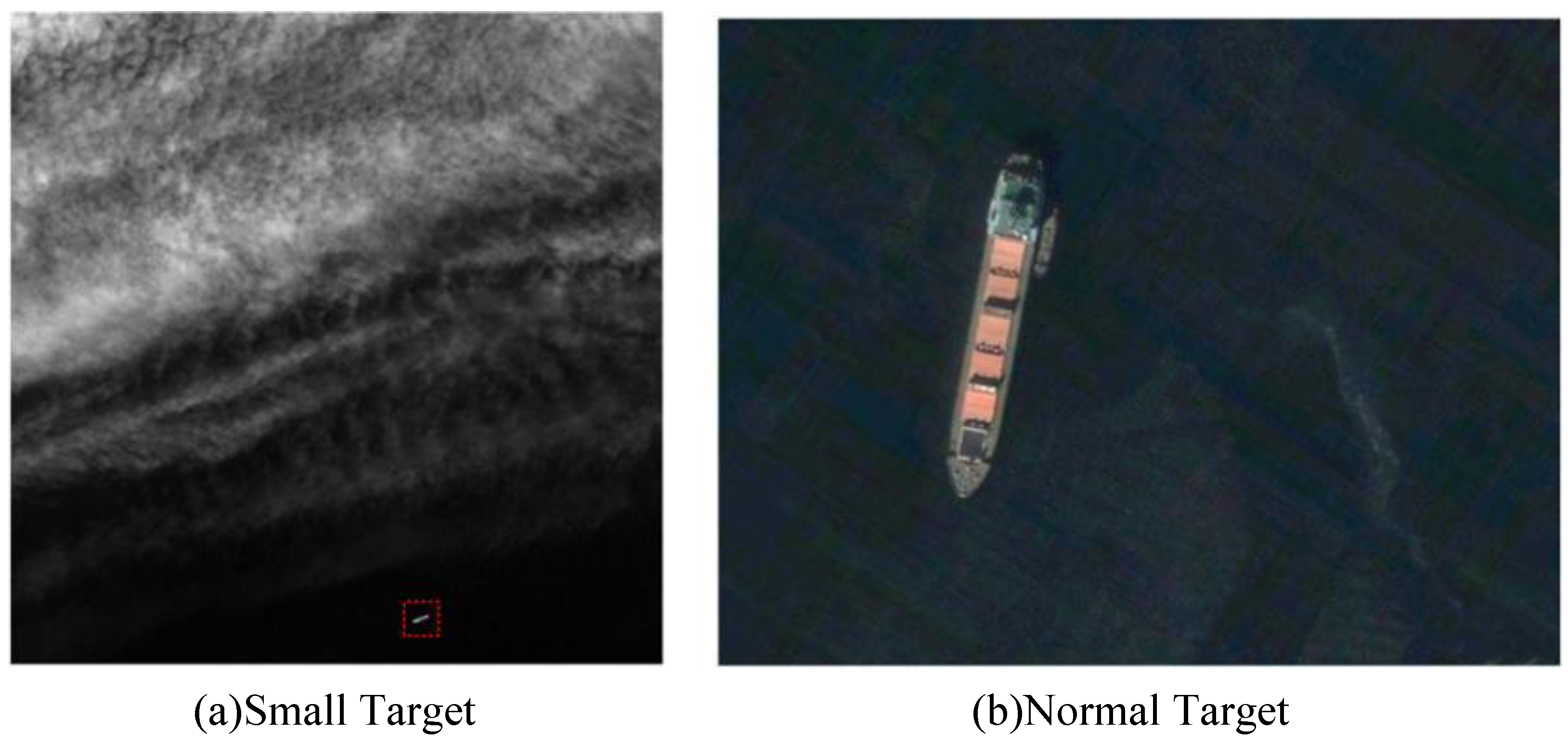
1. Introduction
2. Related Works
2.1. Object Detection
2.2. Ship Target Detection

| Categories | Feature Extraction Enhancement | Multi-Scale | Improved Bounding Box Regression | Robustness Enhancement | Imbalanced Learning |
|---|---|---|---|---|---|
| Related Works | [25,27] | [25,26,30,31,32] | [27,29] | [28,32] | [34,35] |
| Our Methods | – | – | Adopt NWD Loss for Regression Optimization | Oversampling for Robustness in Complex Scenes | Cost-sensitive Function + Oversampling |
2.3. Imbalanced Learning in Object Detection
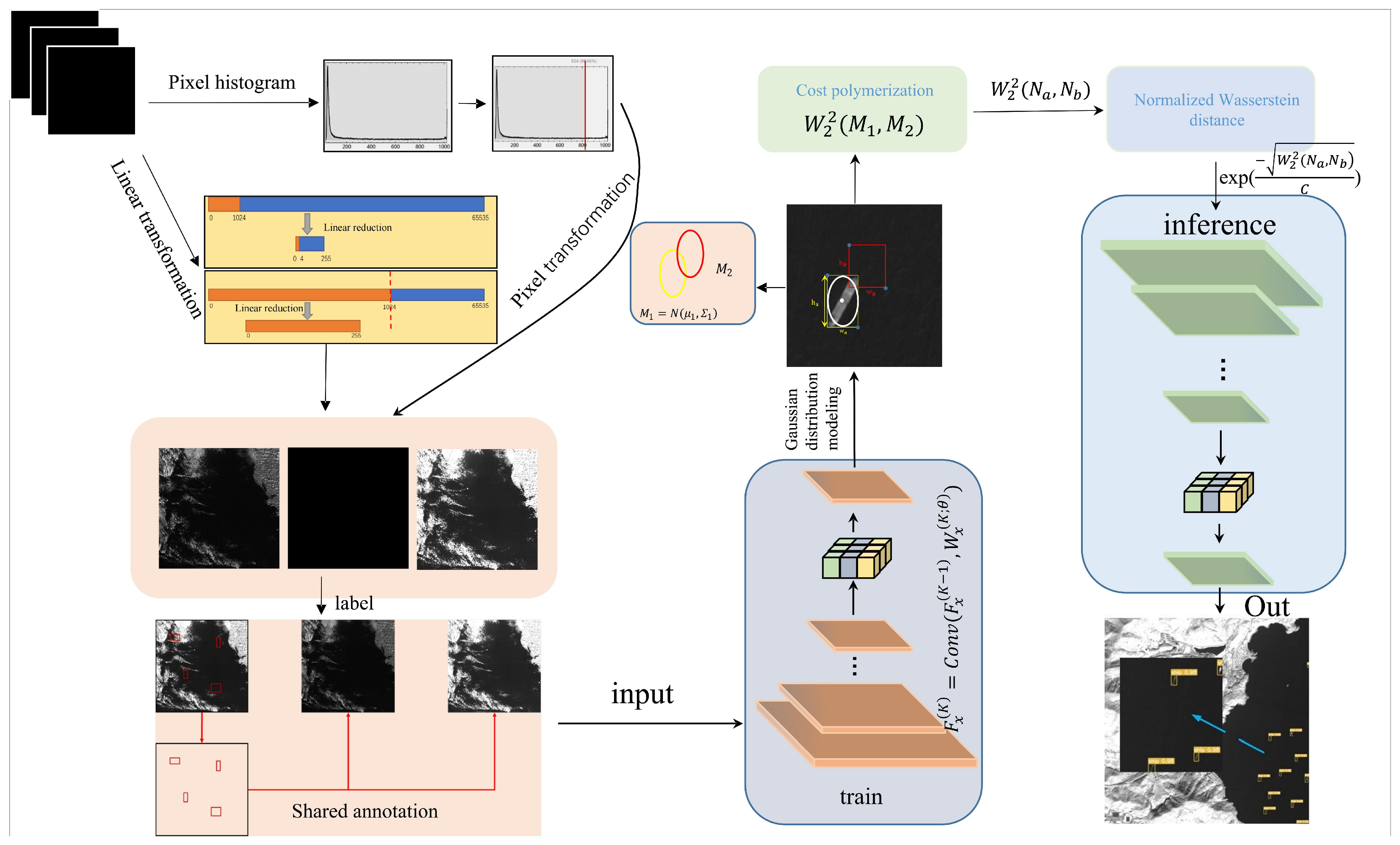
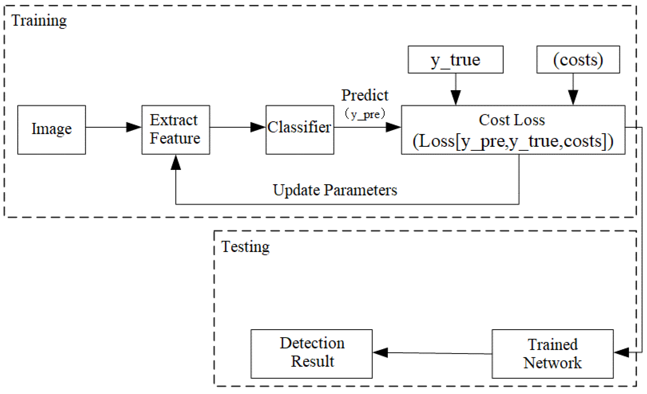
3. Proposed Method
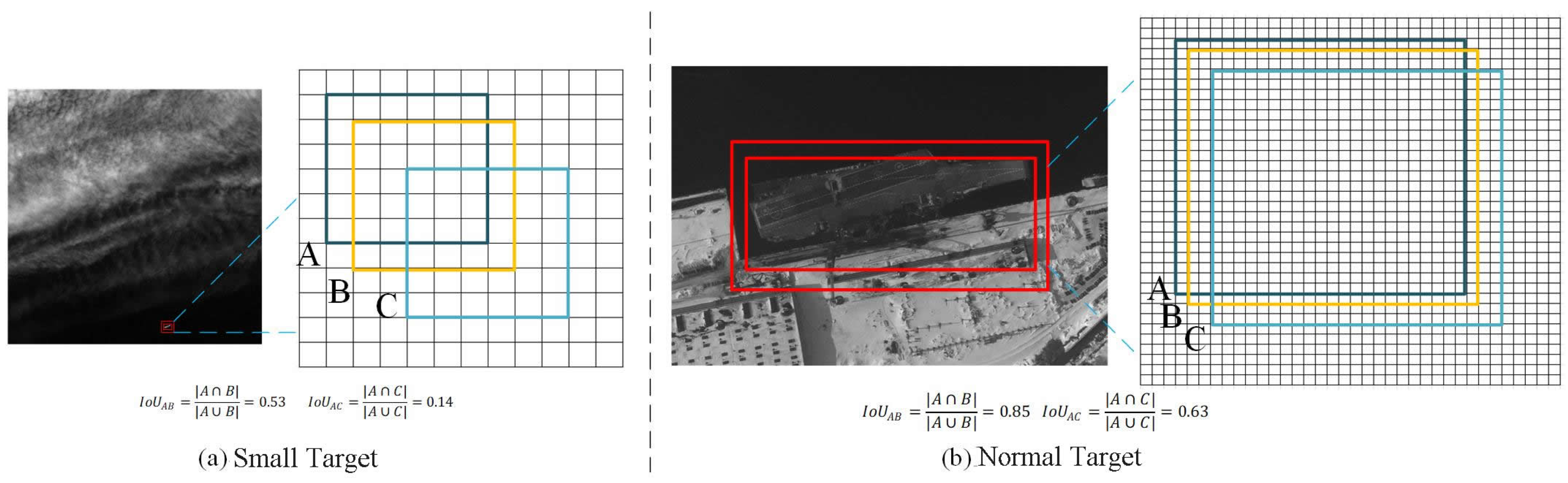
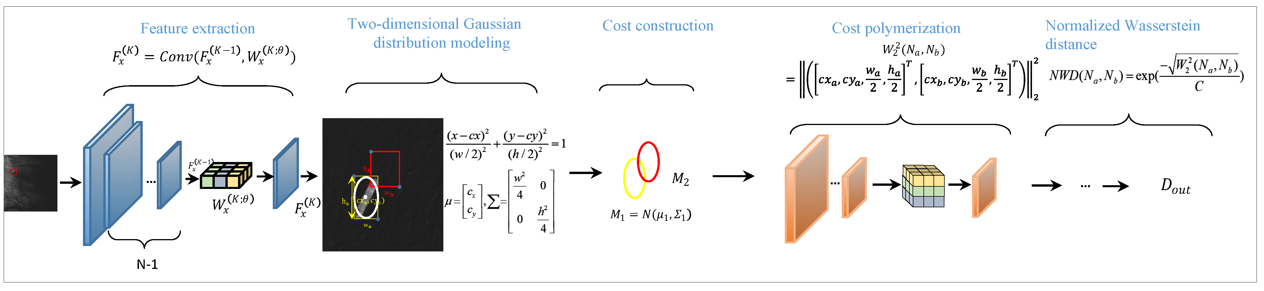
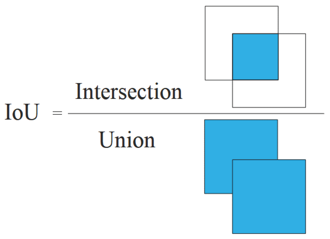
3.1. IoU-Based Cost-Sensitive Improvements
3.2. Design of a Cost-Sensitive Function Based on Imbalanced Learning
3.2.1. Cost Sensitivity Based on Binary Cross-Entropy Loss
| Algorithm 1 Cost-sensitive YOLOv7 object detection algorithm | |
| Require: High-resolution satellite remote sensing ship images | |
| Ensure: Ship detection result map | |
| Preprocessing: Data augmentation operations such as Mosaic and random cropping | |
| Initialisation: Initialise YOLOv7 and weights | |
| Training: | |
| for each training iteration do | |
| 1. The YOLOv7 extracts image features and performs classification predictions | |
| 2. Use the ground truth and predictions to the cost-sensitive function to calculate the loss value | |
| 3. Backpropagate the loss and optimise the parameters using the SGD optimiser | |
| 4. After each iteration, evaluate performance using validation set and calculate metrics | |
| 5. Based on the validation set performance, update the weight file, compare the current parameters with the previous iteration’s parameters, and retain the better parameters | |
| end for | |
| Testing: | |
| Input the remote sensing ship test set images and use the trained model for testing to obtain the final detection result image | |
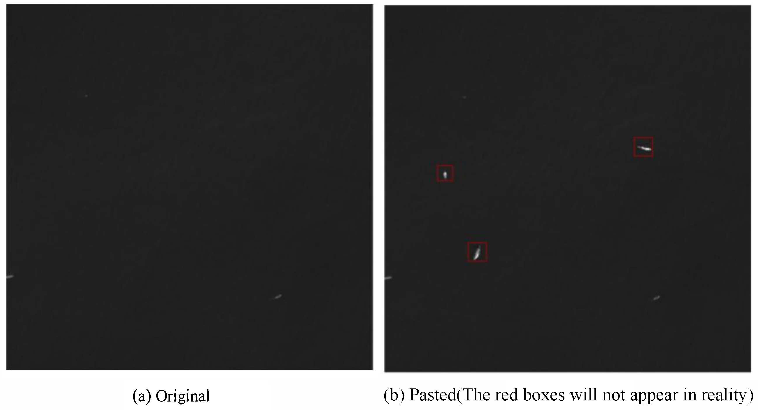
3.2.2. Oversampling
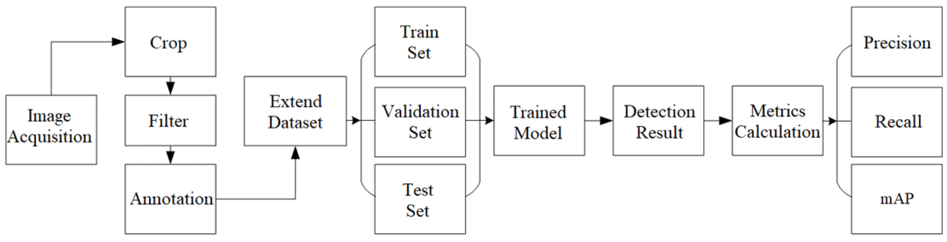
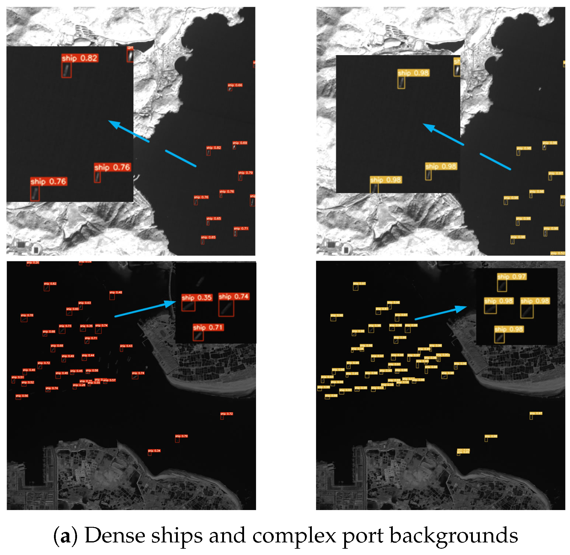
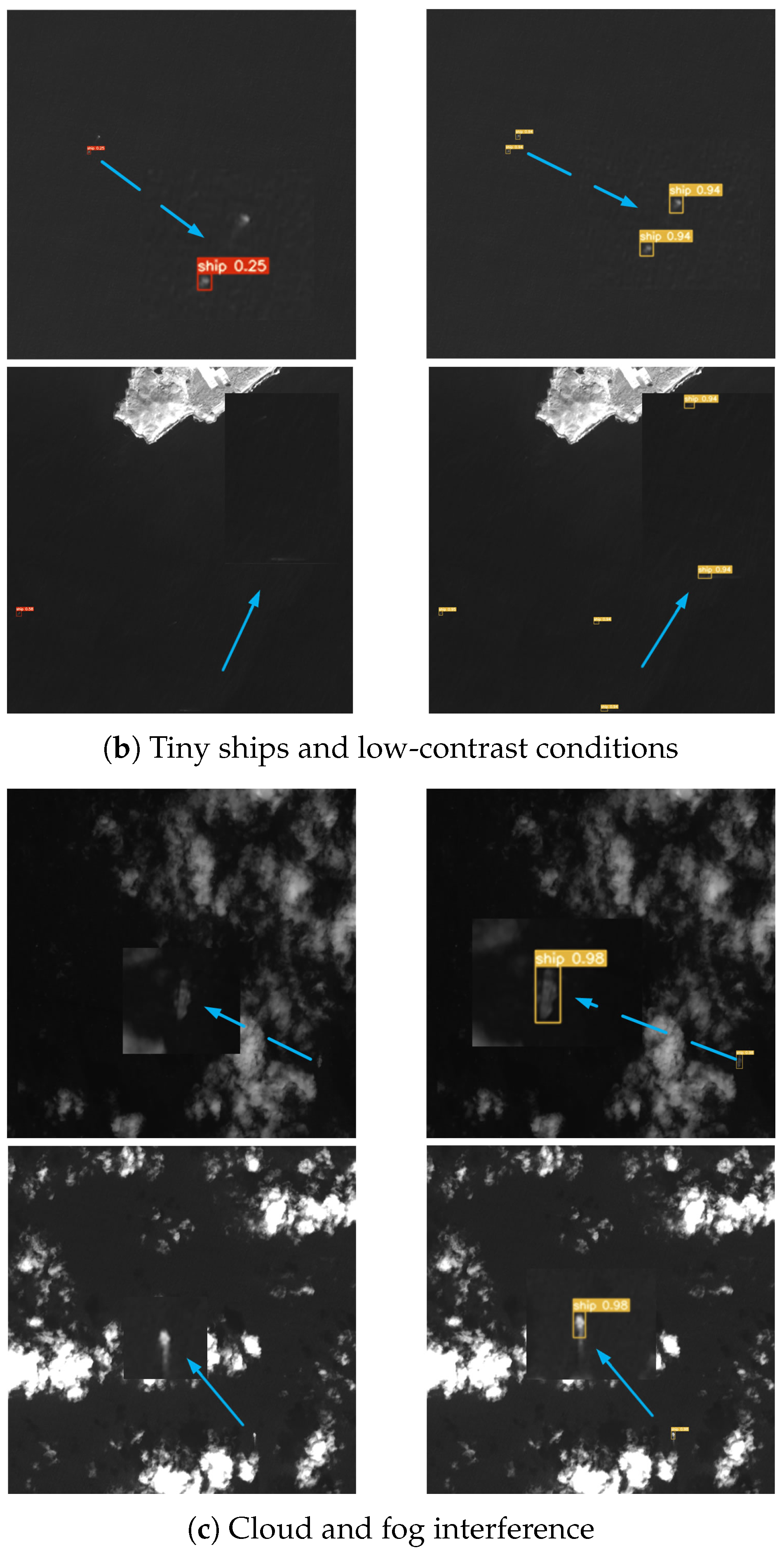
4. Experiments and Analysis
4.1. Implementation Details
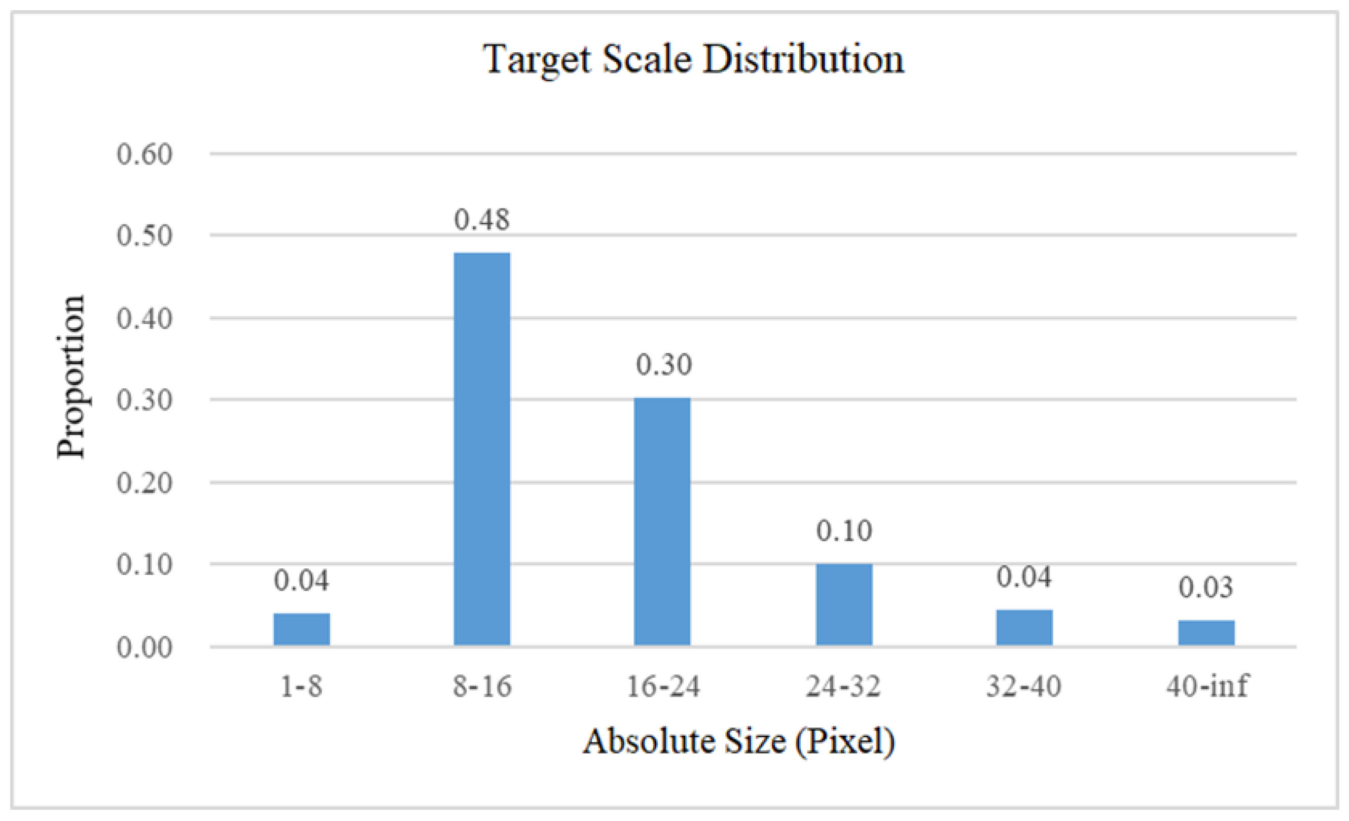
4.2. Datasets
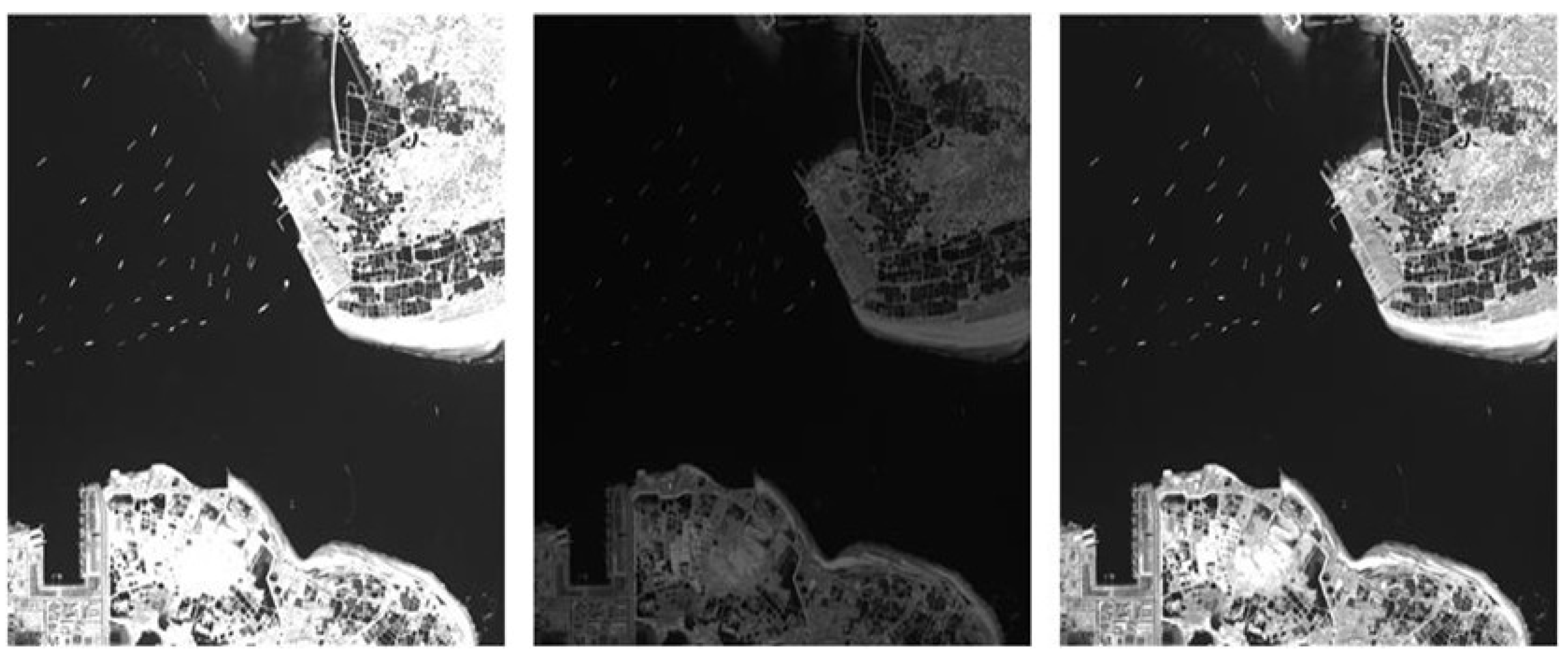
4.3. Experimental Results and Analysis of IoU-Based Cost-Sensitive Improvements
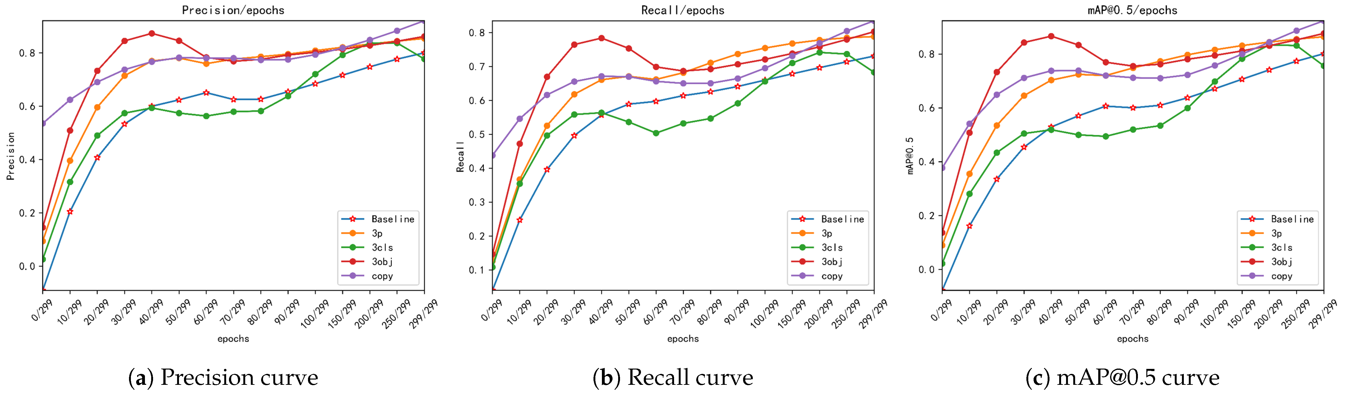
4.4. Experimental Validation of Cost-Sensitive Function Design Based on Imbalanced Learning
5. Discussions
5.1. Comparison with Prior Research
5.2. Significance of Research Findings
5.3. Limitations of the Study
5.4. Future Research Directions
6. Conclusions
Author Contributions
Funding
Data Availability Statement
Acknowledgments
Conflicts of Interest
References
- Zhang, M.; Zhang, R.; Yang, Y.; Bai, H.; Zhang, J.; Guo, J. ISNet: Shape matters for infrared small target detection. In Proceedings of the IEEE/CVF Conference on Computer Vision and Pattern Recognition, New Orleans, LA, USA, 18–24 June 2022; pp. 877–886. [Google Scholar]
- Zhang, M.; Zhang, R.; Zhang, J.; Guo, J.; Li, Y.; Gao, X. Dim2Clear Network for Infrared Small Target Detection. IEEE Trans. Geosci. Remote Sens. 2023, 61, 5001714. [Google Scholar] [CrossRef]
- Wu, W.; Fan, X.; Hu, Z.; Zhao, Y. CGDU-DETR: An End-to-End Detection Model for Ship Detection in Day–Night Transition Environments. J. Mar. Sci. Eng. 2025, 13, 1155. [Google Scholar] [CrossRef]
- Chen, L.; Hu, Z.; Chen, J.; Sun, Y. SVIADF: Small Vessel Identification and Anomaly Detection Based on Wide-Area Remote Sensing Imagery and AIS Data Fusion. Remote Sens. 2025, 17, 868. [Google Scholar] [CrossRef]
- Yu, C.; Liu, Y.; Wu, S.; Xia, X.; Hu, Z.; Lan, D.; Liu, X. Pay attention to local contrast learning networks for infrared small target detection. IEEE Geosci. Remote Sens. Lett. 2022, 19, 3512705. [Google Scholar] [CrossRef]
- Li, H.; Yu, R.; Ding, W. Research development of small object traching based on deep learning. Acta Aeronaut. Astronaut. Sin. 2021, 42, 1000–6893. [Google Scholar]
- Girshick, R.; Donahue, J.; Darrell, T.; Malik, J. Rich feature hierarchies for accurate object detection and semantic segmentation. In Proceedings of the IEEE Conference on Computer Vision and Pattern Recognition, Columbus, OH, USA, 23–28 June 2014; pp. 580–587. [Google Scholar]
- He, K.; Zhang, X.; Ren, S.; Sun, J. Spatial pyramid pooling in deep convolutional networks for visual recognition. IEEE Trans. Pattern Anal. Mach. Intell. 2015, 37, 1904–1916. [Google Scholar] [CrossRef] [PubMed]
- Girshick, R. Fast R-CNN. In Proceedings of the IEEE International Conference on Computer Vision, Santiago, Chile, 7–13 December 2015; pp. 1440–1448. [Google Scholar]
- Ren, S.; He, K.; Girshick, R.; Sun, J. Faster R-CNN: Towards real-time object detection with region proposal networks. IEEE Trans. Pattern Anal. Mach. Intell. 2016, 39, 1137–1149. [Google Scholar] [CrossRef] [PubMed]
- Lin, T.Y.; Dollár, P.; Girshick, R.; He, K.; Hariharan, B.; Belongie, S. Feature pyramid networks for object detection. In Proceedings of the IEEE Conference on Computer Vision and Pattern Recognition, Honolulu, HI, USA, 21–26 July 2017; pp. 2117–2125. [Google Scholar]
- Redmon, J.; Divvala, S.; Girshick, R.; Farhadi, A. You only look once: Unified, real-time object detection. In Proceedings of the IEEE Conference on Computer Vision and Pattern Recognition, Las Vegas, NV, USA, 27–30 June 2016; pp. 779–788. [Google Scholar]
- Wang, C.Y.; Bochkovskiy, A.; Liao, H.Y.M. YOLOv7: Trainable bag-of-freebies sets new state-of-the-art for real-time object detectors. In Proceedings of the IEEE/CVF Conference on Computer Vision and Pattern Recognition, Vancouver, BC, Canada, 17–24 June 2023; pp. 7464–7475. [Google Scholar]
- Liu, W.; Anguelov, D.; Erhan, D.; Szegedy, C.; Reed, S.; Fu, C.Y.; Berg, A.C. SSD: Single shot multibox detector. In Proceedings of the Computer Vision–ECCV 2016: 14th European Conference, Amsterdam, The Netherlands, 11–14 October 2016; Springer: Cham, Switzerland, 2016. Part I. pp. 21–37. [Google Scholar]
- Carion, N.; Massa, F.; Synnaeve, G.; Usunier, N.; Kirillov, A.; Zagoruyko, S. End-to-end object detection with transformers. In Proceedings of the European Conference on Computer Vision, Glasgow, UK, 23–28 August 2020; Springer: Cham, Switzerland, 2020; pp. 213–229. [Google Scholar]
- Lin, T.Y.; Maire, M.; Belongie, S.; Hays, J.; Perona, P.; Ramanan, D.; Dollár, P.; Zitnick, C.L. Microsoft coco: Common objects in context. In Proceedings of the Computer Vision–ECCV 2014: 13th European Conference, Zurich, Switzerland, 6–12 September 2014; Springer: Cham, Switzerland, 2014. Part V. pp. 740–755. [Google Scholar]
- Zhang, M.; Bai, H.; Zhang, J.; Zhang, R.; Wang, C.; Guo, J.; Gao, X. RKformer: Runge-Kutta Transformer with Random-Connection Attention for Infrared Small Target Detection. In Proceedings of the MM ’22: Proceedings of the 30th ACM International Conference on Multimedia, Lisboa, Portugal, 10–14 October 2022; pp. 1730–1738. [Google Scholar] [CrossRef]
- Zhang, M.; Yang, H.; Guo, J.; Li, Y.; Gao, X.; Zhang, J. IRPruneDet: Efficient infrared small target detection via wavelet structure-regularized soft channel pruning. In Proceedings of the AAAI Conference on Artificial Intelligence, Vancouver, BC, Canada, 20–27 February 2024; Volume 38, pp. 7224–7232. [Google Scholar]
- Zhang, J.; Zhang, R.; Xu, L.; Lu, X.; Yu, Y.; Xu, M.; Zhao, H. Fastersal: Robust and real-time single-stream architecture for RGB-D salient object detection. IEEE Trans. Multimed. 2024, 27, 2477–2488. [Google Scholar] [CrossRef]
- Zhang, R.; Yang, B.; Xu, L.; Huang, Y.; Xu, X.; Zhang, Q.; Jiang, Z.; Liu, Y. A benchmark and frequency compression method for infrared few-shot object detection. IEEE Trans. Geosci. Remote Sens. 2025, 63, 5001711. [Google Scholar] [CrossRef]
- Cheng, G.; Yuan, X.; Yao, X.; Yan, K.; Zeng, Q.; Xie, X.; Han, J. Towards large-scale small object detection: Survey and benchmarks. IEEE Trans. Pattern Anal. Mach. Intell. 2023, 45, 13467–13488. [Google Scholar] [CrossRef] [PubMed]
- Sun, Y.; Zhao, Y.; Hu, Z.; Wu, W.; Xia, J.; Wang, Y. SSRLM: A self-supervised representation learning method for identifying one ship with multi-MMSI codes. Ocean Eng. 2024, 312, 119186. [Google Scholar] [CrossRef]
- Zhang, R.; Cao, Z.; Huang, Y.; Yang, S.; Xu, L.; Xu, M. Visible-infrared person re-identification with real-world label noise. IEEE Trans. Circuits Syst. Video Technol. 2025, 35, 4857–4869. [Google Scholar] [CrossRef]
- Zhang, M.; Wang, Y.; Guo, J.; Li, Y.; Gao, X.; Zhang, J. IRSAM: Advancing segment anything model for infrared small target detection. In Proceedings of the European Conference on Computer Vision, Milan, Italy, 29 September–4 October 2024; Springer: Cham, Switzerland, 2024; pp. 233–249. [Google Scholar] [CrossRef]
- Zheng, Z.; Zhong, Y.; Ma, A.; Han, X.; Zhao, J.; Liu, Y.; Zhang, L. HyNet: Hyper-scale object detection network framework for multiple spatial resolution remote sensing imagery. ISPRS J. Photogramm. Remote Sens. 2020, 166, 1–14. [Google Scholar] [CrossRef]
- Wang, P.; Sun, X.; Diao, W.; Fu, K. FMSSD: Feature-merged single-shot detection for multiscale objects in large-scale remote sensing imagery. IEEE Trans. Geosci. Remote Sens. 2019, 58, 3377–3390. [Google Scholar] [CrossRef]
- Zhang, X.; Zhang, S.; Sun, Z.; Liu, C.; Sun, Y.; Ji, K.; Kuang, G. Cross-sensor SAR image target detection based on dynamic feature discrimination and center-aware calibration. IEEE Trans. Geosci. Remote Sens. 2025, 63, 5209417. [Google Scholar] [CrossRef]
- Dong, Z.; Wang, M.; Wang, Y.; Zhu, Y.; Zhang, Z. Object detection in high resolution remote sensing imagery based on convolutional neural networks with suitable object scale features. IEEE Trans. Geosci. Remote Sens. 2019, 58, 2104–2114. [Google Scholar] [CrossRef]
- Zhang, Y.; Sheng, W.; Jiang, J.; Jing, N.; Wang, Q.; Mao, Z. Priority branches for ship detection in optical remote sensing images. Remote Sens. 2020, 12, 1196. [Google Scholar] [CrossRef]
- Yu, Y.; Ai, H.; He, X.; Yu, S.; Zhong, X.; Lu, M. Ship detection in optical satellite images using Haar-like features and periphery-cropped neural networks. IEEE Access 2018, 6, 71122–71131. [Google Scholar] [CrossRef]
- Wang, Y.; Dong, Z.; Zhu, Y. Multiscale block fusion object detection method for large-scale high-resolution remote sensing imagery. IEEE Access 2019, 7, 99530–99539. [Google Scholar] [CrossRef]
- Sun, Z.; Leng, X.; Zhang, X.; Zhou, Z.; Xiong, B.; Ji, K.; Kuang, G. Arbitrary-direction SAR ship detection method for multi-scale imbalance. IEEE Trans. Geosci. Remote Sens. 2025, 63, 5208921. [Google Scholar] [CrossRef]
- Wu, Y.; Wang, J.; Yang, L.; Yu, M. Survey on Cost-sensitive Deep Learning Methods. Comput. Sci. 2019, 46, 1–12. [Google Scholar]
- Zhang, X.L. Speech separation by cost-sensitive deep learning. In Proceedings of the 2017 Asia-Pacific Signal and Information Processing Association Annual Summit and Conference (APSIPA ASC), Kuala Lumpur, Malaysia, 12–15 December 2017; pp. 159–162. [Google Scholar]
- Jiang, J.; Liu, X.; Zhang, K.; Long, E.; Wang, L.; Li, W.; Liu, L.; Wang, S.; Zhu, M.; Cui, J.; et al. Automatic diagnosis of imbalanced ophthalmic images using a cost-sensitive deep convolutional neural network. Biomed. Eng. Online 2017, 16, 1–20. [Google Scholar] [CrossRef] [PubMed]
- Zhao, Y.; Chen, S.; Liu, S.; Hu, Z.; Xia, J. Hierarchical equalization loss for long-tailed instance segmentation. IEEE Trans. Multimed. 2024, 26, 6943–6955. [Google Scholar] [CrossRef]
- Chawla, N.V.; Bowyer, K.W.; Hall, L.O.; Kegelmeyer, W.P. SMOTE: Synthetic minority over-sampling technique. J. Artif. Intell. Res. 2002, 16, 321–357. [Google Scholar] [CrossRef]
- Garcia, E.A.; He, H. Learning from Imbalanced Data. IEEE Trans. Knowl. Data Eng. 2009, 21, 1263–1284. [Google Scholar] [CrossRef]
- Buda, M.; Maki, A.; Mazurowski, M.A. A systematic study of the class imbalance problem in convolutional neural networks. Neural Netw. Off. J. Int. Neural Netw. Soc. 2018, 106, 249–259. [Google Scholar] [CrossRef] [PubMed]
- Liao, J.; Zhao, Y.; Xia, J.; Gu, Y.; Hu, Z.; Wu, W. Dynamic-Equalized-Loss Based Learning Framework for Identifying the Behavior of Pair-Trawlers. In Proceedings of the International Conference on Intelligent Computing, Tianjin, China, 5–8 August 2024; Springer: Singapore, 2024; pp. 337–349. [Google Scholar] [CrossRef]
- Fan, X.; Hu, Z.; Zhao, Y.; Chen, J.; Wei, T.; Huang, Z. A small ship object detection method for satellite remote sensing data. IEEE J. Sel. Top. Appl. Earth Obs. Remote Sens. 2024, 17, 11886–11898. [Google Scholar] [CrossRef]
- Wang, J.; Xu, C.; Yang, W.; Yu, L. A normalized Gaussian Wasserstein distance for tiny object detection. arXiv 2021, arXiv:2110.13389. [Google Scholar]
- Chen, J.; Hu, Z.; Wu, W.; Zhao, Y.; Huang, B. LKPF-YOLO: A Small Target Ship Detection Method for Marine Wide-Area Remote Sensing Images. IEEE Trans. Aerosp. Electron. Syst. 2024, 61, 2769–2783. [Google Scholar] [CrossRef]
- Zhou, D.; Fang, J.; Song, X.; Guan, C.; Yin, J.; Dai, Y.; Yang, R. IoU loss for 2D/3D object detection. In Proceedings of the 2019 International Conference on 3D Vision (3DV), Quebec City, QC, Canada, 16–19 September 2019; pp. 85–94. [Google Scholar]
- Rezatofighi, H.; Tsoi, N.; Gwak, J.; Sadeghian, A.; Reid, I.; Savarese, S. Generalized intersection over union: A metric and a loss for bounding box regression. In Proceedings of the IEEE/CVF Conference on Computer Vision and Pattern Recognition, Long Beach, CA, USA, 15–20 June 2019; pp. 658–666. [Google Scholar]
- Zheng, Z.; Wang, P.; Liu, W.; Li, J.; Ye, R.; Ren, D. Distance-IoU loss: Faster and better learning for bounding box regression. In Proceedings of the AAAI Conference on Artificial Intelligence, New York, NY, USA, 7–12 February 2020; Volume 34, pp. 12993–13000. [Google Scholar]
- Zheng, Z.; Wang, P.; Ren, D.; Liu, W.; Ye, R.; Hu, Q.; Zuo, W. Enhancing geometric factors in model learning and inference for object detection and instance segmentation. IEEE Trans. Cybern. 2021, 52, 8574–8586. [Google Scholar] [CrossRef] [PubMed]
- Kisantal, M.; Wojna, Z.; Murawski, J.; Naruniec, J.; Cho, K. Augmentation for small object detection. arXiv 2019, arXiv:1902.07296. [Google Scholar]
- Jocher, G. YOLOv5 by Ultralytics. Zenodo 2021. [Google Scholar] [CrossRef]
- Jocher, G.; Qiu, J.; Chaurasia, A. YOLOv8 by Ultralytics. 2023. Available online: https://docs.ultralytics.com/models/yolov8 (accessed on 14 June 2025).
- Quan, P.; Lou, Y.; Lin, H.; Liang, Z.; Wei, D.; Di, S. Research on identification and location of charging ports of multiple electric vehicles based on SFLDLC-CBAM-YOLOV7-Tinp-CTMA. Electronics 2023, 12, 1855. [Google Scholar] [CrossRef]
- Wang, C.; He, W.; Nie, Y.; Guo, J.; Liu, C.; Wang, Y.; Han, K. Gold-YOLO: Efficient object detector via gather-and-distribute mechanism. Adv. Neural Inf. Process. Syst. 2023, 36, 51094–51112. [Google Scholar]
- Zhao, Y.; Lv, W.; Xu, S.; Wei, J.; Wang, G.; Dang, Q.; Liu, Y.; Chen, J. Detrs beat yolos on real-time object detection. In Proceedings of the IEEE/CVF Conference on Computer Vision and Pattern Recognition, Seattle, WA, USA, 16–22 June 2024; pp. 16965–16974. [Google Scholar]
- Wang, A.; Chen, H.; Liu, L.; Chen, K.; Lin, Z.; Han, J.; Ding, G. Yolov10: Real-time end-to-end object detection. Adv. Neural Inf. Process. Syst. 2024, 37, 107984–108011. [Google Scholar]
- Khanam, R.; Hussain, M. Yolov11: An overview of the key architectural enhancements. arXiv 2024, arXiv:2410.17725. [Google Scholar]
- Yu, C.; Liu, Y.; Wu, S.; Hu, Z.; Xia, X.; Lan, D.; Liu, X. Infrared small target detection based on multiscale local contrast learning networks. Infrared Phys. Technol. 2022, 123, 104107. [Google Scholar] [CrossRef]
- Liu, J. Ship Detection and Recognition in Optical Remote Sensing Images Based on Deep Neural Networks. Master’s Thesis, Xidian University, Xi’an, China, 2021. [Google Scholar]
- Pazhani, A.A.J.; Periyanayagi, S. A novel haze removal computing architecture for remote sensing images using multi-scale Retinex technique. Earth Sci. Inform. 2022, 15, 1147–1154. [Google Scholar] [CrossRef]
| Method | Precision | Recall | mAP@0.5:0.95 | |
|---|---|---|---|---|
| YOLOv5s [49] | 0.859 | 0.851 | 0.892 | 0.448 |
| CBAM-YOLOv7 [51] | 0.841 | 0.811 | 0.862 | 0.414 |
| YOLOv7x [13] | 0.848 | 0.782 | 0.857 | 0.398 |
| YOLOv7 [13] | 0.864 | 0.766 | 0.841 | 0.405 |
| YOLOv8 [50] | 0.910 | 0.904 | 0.944 | 0.569 |
| GOLD-YOLO [52] | 0.897 | 0.890 | 0.930 | 0.527 |
| RT-Detr [53] | 0.959 | 0.928 | 0.958 | 0.594 |
| YOLOv10 [54] | 0.927 | 0.940 | 0.964 | 0.617 |
| YOLOv11 [55] | 0.927 | 0.938 | 0.966 | 0.605 |
| YOLOv10 (NWD) | 0.950 | 0.917 | 0.963 | 0.601 |
| YOLOv11 (NWD) | 0.911 | 0.910 | 0.952 | 0.570 |
| YOLOv7 (NWD) | 0.967 | 0.958 | 0.971 | 0.588 |
| Ratio | Precision | Recall | mAP@0.5 | mAP@0.5:0.95 |
|---|---|---|---|---|
| 0.0 | 0.864 | 0.766 | 0.841 | 0.405 |
| 0.1 | 0.824 | 0.842 | 0.875 | 0.410 |
| 0.2 | 0.854 | 0.802 | 0.861 | 0.401 |
| 0.3 | 0.885 | 0.848 | 0.899 | 0.438 |
| 0.4 | 0.882 | 0.861 | 0.897 | 0.446 |
| 0.5 | 0.922 | 0.895 | 0.937 | 0.501 |
| 0.6 | 0.944 | 0.949 | 0.962 | 0.572 |
| 0.7 | 0.958 | 0.963 | 0.976 | 0.601 |
| 0.8 | 0.974 | 0.969 | 0.979 | 0.646 |
| 0.9 | 0.977 | 0.963 | 0.977 | 0.640 |
| 1.0 | 0.967 | 0.958 | 0.971 | 0.588 |
| Method | Precision | Recall | mAP@0.5 | mAP@0.5:0.95 |
|---|---|---|---|---|
| Baseline(1,1) | 0.837 | 0.682 | 0.764 | 0.364 |
| copy | 0.834 | 0.831 | 0.861 | 0.376 |
| 3,3 | 0.861 | 0.771 | 0.847 | 0.407 |
| 3,1 | 0.814 | 0.705 | 0.783 | 0.366 |
| 1,3 | 0.855 | 0.770 | 0.856 | 0.410 |
Disclaimer/Publisher’s Note: The statements, opinions and data contained in all publications are solely those of the individual author(s) and contributor(s) and not of MDPI and/or the editor(s). MDPI and/or the editor(s) disclaim responsibility for any injury to people or property resulting from any ideas, methods, instructions or products referred to in the content. |
© 2025 by the authors. Licensee MDPI, Basel, Switzerland. This article is an open access article distributed under the terms and conditions of the Creative Commons Attribution (CC BY) license (https://creativecommons.org/licenses/by/4.0/).
Share and Cite
Hu, Z.; Wu, W.; Yang, Z.; Zhao, Y.; Xu, L.; Kong, L.; Chen, Y.; Chen, L.; Liu, G. A Cost-Sensitive Small Vessel Detection Method for Maritime Remote Sensing Imagery. Remote Sens. 2025, 17, 2471. https://doi.org/10.3390/rs17142471
Hu Z, Wu W, Yang Z, Zhao Y, Xu L, Kong L, Chen Y, Chen L, Liu G. A Cost-Sensitive Small Vessel Detection Method for Maritime Remote Sensing Imagery. Remote Sensing. 2025; 17(14):2471. https://doi.org/10.3390/rs17142471
Chicago/Turabian StyleHu, Zhuhua, Wei Wu, Ziqi Yang, Yaochi Zhao, Lewei Xu, Lingkai Kong, Yunpei Chen, Lihang Chen, and Gaosheng Liu. 2025. "A Cost-Sensitive Small Vessel Detection Method for Maritime Remote Sensing Imagery" Remote Sensing 17, no. 14: 2471. https://doi.org/10.3390/rs17142471
APA StyleHu, Z., Wu, W., Yang, Z., Zhao, Y., Xu, L., Kong, L., Chen, Y., Chen, L., & Liu, G. (2025). A Cost-Sensitive Small Vessel Detection Method for Maritime Remote Sensing Imagery. Remote Sensing, 17(14), 2471. https://doi.org/10.3390/rs17142471