Quantifying Multifactorial Drivers of Groundwater–Climate Interactions in an Arid Basin Based on Remote Sensing Data

Abstract

Groundwater systems are intrinsically linked to climate, with changing conditions significantly altering recharge, storage, and discharge processes, thereby impacting water availability and ecosystem integrity. Critical knowledge gaps persist regarding groundwater equilibrium timescales, water table dynamics, and their governing factors. This study develops a novel remote sensing framework to quantify factor controls on groundwater–climate interaction characteristics in the Heihe River Basin (HRB). High-resolution (0.005° × 0.005°) maps of groundwater response time (GRT) and water table ratio (WTR) were generated using multi-source geospatial data. Employing Geographical Convergent Cross Mapping (GCCM), we established causal relationships between GRT/WTR and their drivers, identifying key influences on groundwater dynamics. Generalized Additive Models (GAM) further quantified the relative contributions of climatic (precipitation, temperature), topographic (DEM, TWI), geologic (hydraulic conductivity, porosity, vadose zone thickness), and vegetative (NDVI, root depth, soil water) factors to GRT/WTR variability. Results indicate an average GRT of ~6.5 × 10⁸ years, with 7.36% of HRB exhibiting sub-century response times and 85.23% exceeding 1000 years. Recharge control dominates shrublands, wetlands, and croplands (WTR < 1), while topography control prevails in forests and barelands (WTR > 1). Key factors collectively explain 86.7% (GRT) and 75.9% (WTR) of observed variance, with spatial GRT variability driven primarily by hydraulic conductivity (34.3%), vadose zone thickness (13.5%), and precipitation (10.8%), while WTR variation is controlled by vadose zone thickness (19.2%), topographic wetness index (16.0%), and temperature (9.6%). These findings provide a scientifically rigorous basis for prioritizing groundwater conservation zones and designing climate-resilient water management policies in arid endorheic basins, with our high-resolution causal attribution framework offering transferable methodologies for global groundwater vulnerability assessments.

1. Introduction

Groundwater systems are in dynamic equilibrium with the climate with numerous feedback [1,2,3]. Under changing climatic conditions, the spatial distribution of natural groundwater recharge is altered, leading to shifts in groundwater storage, water table elevations, and groundwater discharge [4]. These spatio-temporal changes are central to regulating the exchange of moisture and energy across the Earth’s surface, influencing critical processes such as hydro-ecology, carbon cycling, and nutrient dynamics, ultimately affecting the availability of water for human use in integrated water–energy systems [5,6,7,8,9,10,11]. Although the impacts and feedback between various components of the climate system and groundwater have been well-documented, many bidirectional interactions remain inadequately understood [12,13,14]. This knowledge gap is particularly critical in arid regions where groundwater–climate couplings are both scientifically complex and socioeconomically vital [15,16]. The urgency of addressing these uncertainties is underscored by growing global vulnerability: from overdrawn aquifers in intensively managed basins across North America to emerging crises in hyper-arid zones of South America, where deteriorating ecosystems, governance challenges, and climatic stressors converge to threaten groundwater sustainability [17,18,19,20,21,22,23].

Transient groundwater flow conditions, which are time-dependent, are notably more complex than steady-state conditions [24]. As such, quantifying the time-dependent hydraulic response of aquifers is essential for understanding the role of transience in hydrogeological systems, particularly in groundwater management. In parallel, characterizing the water table is critical for understanding the interactions between groundwater, surface water, ecosystems, and climate [25]. Differentiating water table types is a key step in conceptualizing regional groundwater flow systems and gaining deeper insight into groundwater–topography–climate interactions [26]. Therefore, accurately assessing groundwater equilibrium timescales and water table types at regional scales is fundamental for determining the appropriate timeframe and spatial scope for considering an aquifer’s response to change [27,28,29,30,31]. Addressing these challenges requires regionally tailored approaches, especially in hydrologically sensitive arid basins [32].

The Heihe River Basin (HRB) exemplifies such critical arid regions where groundwater-climate interactions demand urgent scientific attention [33,34,35]. As the second-largest endorheic basin in northwest China, the HRB presents a quintessential case study of groundwater-climate coupling under extreme aridity. Its hydrological gradients, from alpine headwaters to terminal deserts, create a natural laboratory for studying recharge–discharge dynamics [36,37]. Simultaneously, rapid population growth and agricultural expansion have intensified groundwater stress, with water tables declining in critical zones [15,38]. This combination of scientific representativeness and management urgency positions the HRB as an ideal model system for advancing groundwater–climate research in arid endorheic basins globally [39,40,41,42].

In recent decades, various geomatic synthesis metrics, including groundwater response time (GRT) and water table ratio (WTR), have been introduced to quantify the interactions between groundwater, topography, and climate [43,44,45,46,47,48,49]. For example, continental- to global-scale studies by Gleeson et al. (2011) [50] and Cuthbert et al. (2019) [51] pioneered GRT/WTR frameworks but operated at coarse resolutions unsuitable for regional management. Although these efforts have extended GRT and WTR analyses to continental and global scales [50,51], these maps remain coarse in spatial resolution and lack the necessary precision for effective application at regional scales, particularly in arid and semi-arid regions. Furthermore, these global maps do not provide the detailed insights needed to understand the underlying controls or factors that drive groundwater–climate interaction patterns and the hydraulic response timescales of aquifers. Critically, they cannot resolve causal drivers that modulate aquifer sensitivity to climate variability. In this study, “control factors” are defined as the primary environmental determinants—encompassing climatic drivers, topographic gradients, geological structures, and vegetation dynamics—that modulate the sensitivity and response behavior of groundwater systems to climatic variability. Robust quantification of these factors is critical for improving predictive understanding of aquifer resilience under future climate scenarios. Thus, it is essential to develop high-resolution maps of GRT and WTR utilizing multi-source, high-precision local datasets. Meanwhile, clarifying the interactions between GRT, WTR, and their causal relationships with key driving factors is critical for advancing our understanding of groundwater system dynamics [17,19,52,53,54].

To bridge these gaps, this study integrates 0.005° remote sensing data with novel causal inference frameworks; high-resolution GRT and WTR maps were derived from localized variables (porosity, hydraulic conductivity, aquifer thickness, etc.) to investigate spatial coherence across landcovers. This study aims to leverage detailed regional datasets to map groundwater equilibrium timescales and water table types across the HRB. High-resolution data for GRT and WTR (including WTR type) were derived from local variables such as porosity (S), aquifer hydraulic conductivity (K), aquifer thickness (H), distance (L), precipitation (P), aridity index (ϕ), and maximum terrain rise (d). This high-precision mapping enabled an investigation into whether GRT and WTR characteristics are regionally consistent or fragmented across different landcovers. However, the aquifer system response time is typically large, with 75% of the Earth’s land surface exhibiting response times greater than 100 years [51], rendering time series and temporal statistical models impractical for attributing GRT and WTR. Additionally, the complex interplay of multiple influencing factors often leads to weak or insignificant correlations between these factors and the groundwater variables. To address this, the Geographical Convergent Cross Mapping (GCCM) method was employed to explore causal relationships between the influencing factors and GRT or WTR types. Furthermore, the Generalized Additive Model (GAM) was used to quantify the relative contributions of various factors to the total variance in GRT and WTR. Finally, based on these findings, we propose a strategy to better protect natural groundwater systems that are experiencing short-term response time.

Specifically, this study addresses critical knowledge gaps in groundwater–climate interactions for arid endorheic basins by pursuing three specific objectives: (1) develop high-resolution (0.005° × 0.005°) maps of GRT and WTR in the HRB using multi-source remote sensing datasets to overcome the limitations of coarse global-scale products; (2) quantitatively identify causal drivers of groundwater dynamics through GCCM to overcome correlation–conflation issues in complex systems; (3) attribute relative contributions of climatic, topographic, geologic, and vegetative factors to GRT/WTR variability using GAM. By establishing these regional-specific groundwater sensitivity frameworks, we aim to provide transferable methodologies for assessing aquifer vulnerability in water-limited basins worldwide.

2. Materials and Methods

2.1. Study Area

The Heihe River Basin (HRB) (Figure 1a,b), geospatially situated between 97.1°E–102.0°E and 37.7°N–42.7°N, is the second largest endorheic basin in the arid region of northwestern China [34]. The HRB is characterized by an arid continental monsoonal climatic regime, with an annual precipitation exceeding 300 mm within the upstream mountainous region, ranging from 50 to 500 mm in the midstream region, and a meager averaged 42 mm in the downstream desert region [40]. The Heihe River originates in the mountain cryosphere in the Qilian Mountains, which is located on the periphery of the Qinghai-Tibetan Plateau, and follows a northerly trajectory that culminates in its eventual dissipation in terminal lakes nested in the Gobi desert [55]. The HRB has a variety of climate zones, including hyper-arid, arid, semi-arid, dry sub-humid, and humid regions (Figure 1c). The HRB is conventionally divided into the following three distinct sections: the upper reaches (uHRB), which is the water resource formation area; the middle reaches (mHRB), representing the agricultural and human activity zone; and the lower reaches (lHRB), an ecologically sensitive terminal area. Representative vegetation types over the HRB subregions are shown in Figure 1d. As a result, the HRB shows intricate spatial patterns of climate–groundwater interactions, shaped by its expansive size, varied landscape, and the combined effects of climatic variability and human activity [56]. This study focuses on the traditional HRB, extending into some adjacent areas, with the boundaries expanded to include the outermost rectangular region, covering a lateral extent of 5° in both longitude and latitude directions.

2.2. Calculations of WTR and GRT

GRT quantifies the characteristic timescale for an aquifer system to respond significantly to recharge variations, serving as a first-order approximation of hydraulic inertia [57]. Specifically, GRT represents the duration needed for transient flow within heterogeneous porous media to approximate steady-state conditions, often referred to as the system’s hydraulic response time [45,46]. Ref. [49] provided an analytical solution to estimate GRT at high resolution, while Ref. [51] further simplified the equation by linearizing it. The GRT can be expressed mathematically as follows [51,58]:

$$GRT={\displaystyle \frac{S{L}^2}{{\pi }^{2}KH}}$$

(1)

where $L$ (m) represents the distance between perennial streams; $S$ (dimensionless) denotes the aquifer storage coefficient (approximately equal to porosity values); $K$ (m/y) is the aquifer hydraulic conductivity, and $H$ (m) is the aquifer thickness, which can be approximated by the mapped depth to bedrock. A detailed description of GRT can be found in the literature [43,44,45,48,49]. Physically, GRT indicates how rapidly climate signals propagate through aquifers—systems with GRT < 100 years exhibit near-contemporary climate coupling, while GRT > 10,000 years reflect paleowater systems decoupled from modern climate.

WTR characterizes the relative position of the water table within the subsurface profile. It is a dimensionless metric derived through geomatic synthesis to classify water table types and map the dominant modes of groundwater–climate interactions. Specifically, WTR serves as an indicator of the relative saturation of the subsurface, reflecting the degree to which the water table interacts with the underlying topography. The linearized form of the WTR is given by Refs. [50,51,58] as follows:

$$WTR={\displaystyle \frac{L^{2}R}{8KHd}}$$

(2)

where $d$ denotes the maximum terrain rise and $R$ (m/y) is the average annual recharge rate, which can be estimated using the following equation [59]:

$$R=P\times \alpha \left(1-{\displaystyle \frac{\ln \left({\omega }^{\beta }+1\right)}{1+\ln \left({\omega }^{\beta }+1\right)}}\right)$$

(3)

where $P$ is the precipitation (m/y), $\omega$ is the reciprocal of aridity index (dimensionless), calculated as the ratio of precipitation to potential evapotranspiration (PET/P), and $\alpha$ (dimensionless) is a constant representing the fraction of precipitation that becomes recharge under humid conditions ($\omega$ = 0). The characteristic exponent $\beta$ of the aridity index is also included. For this study, values of $\alpha$ = 0.72 and $\beta$ = 15.11 were used, as suggested in previous research [59].

The WTR distinguishes the following two fundamental groundwater–climate interaction modes:

• WTR < 1: Recharge-controlled systems where the water table is deep and climate inputs dominate;
• WTR > 1: Topography-controlled systems with shallow water tables enabling bidirectional land-atmosphere exchanges.

Our classification of water table types follows the globally established framework by Cuthbert et al. (2019) [51]: a WTR greater than one indicates a “topography-controlled” domain, where groundwater dynamics are primarily governed by topographic features. In contrast, a WTR less than one signifies a “recharge-controlled” domain, in which the groundwater system is more influenced by recharge from the climate system. Further details regarding the WTR and its implications can be found in the literature [47,50,51].

Figure 2 summarizes the total data processing workflow. To map the GRT and WTR across the HRB, spatially distributed data for each variable in the respective GRT and WTR equations were derived from geomatic sources, remote sensing products, or representative numerical models. A brief description of these datasets is provided here, with full details available in Supplementary Table S1. The spatial data for each variable were integrated into a unified projection, ensuring consistency in the datum (WGS-84). Using a common projection, the GRT and WTR were computed for each raster pixel via multiplication and division operations performed with ArcGIS 10.6 or MATLAB 2023b.

Specifically, $S$ and $K$ values were sourced from the GLobal HYdrogeology MaPS (GLHYMPS) dataset, which provides unprocessed vector data of global permeability and porosity [60]. $H$ was extracted from a global depth-to-bedrock dataset with a spatial resolution of 250 m [61]. $P$ was derived from a monthly air temperature and precipitation gridded dataset on 0.025° spatial resolution in China [62]. $\omega$ was obtained from a global aridity index and potential evapotranspiration database [63]. $L$ was calculated using a nationally consistent river network, excluding rivers below grade five due to increased data uncertainty. $L$ was determined for each pixel by calculating the shortest Euclidean (straight line) distance between river locations on opposing sides of the pixel, with a low-pass filter applied to remove outliers and speckling. $d$ was calculated using the elevation range derived from ASTER-GDEM data for the Qilian Mountain area. To prevent computational issues, a value of 1 m was added to instances where $d$ was equal to 0.

All variables were clipped to the boundaries of the HRB and resampled to a grid resolution of 0.005° × 0.005°. These variables exhibit spatial heterogeneity, resulting in a distinct calculation of GRT and WTR for each region over the HRB.

2.3. Geographical Convergent Cross Mapping (GCCM)

The GCCM method was applied to identify causal relationships between influencing factors and GRT or WTR type within the HRB. The convergent cross mapping technique is effective in mitigating spurious correlations and extracting robust causality between time-series variables [64]. Building upon this, the GCCM is extended for spatial causal inference, utilizing cross-sectional spatial data to perform cross-mapping predictions within a reconstructed state space [65].

In a dynamic system, if its trajectory converges to an attractor “shadow manifold” $M_{\mathrm{x}}$, for a given $x$, the value of $y$ can be predicted from its close neighbors identified within $M_{\mathrm{x}}$ as represented by Ref. [65]:

$$\widehat{Y_s}|M_x={\displaystyle \sum }_{i=1}^{l+1}\left(W_{s_i}{Y}_{s_i}|M_x\right)$$

(4)

where $s$ denotes a spatial unit for which the value of $Y$ is to be predicted, $\widehat{Y_{\mathrm{s}}}$ represents the predicted value, $\mathrm{l}$ is the embedding dimension, $s_{\mathrm{i}}$ is the spatial unit used for prediction, $W_{\mathrm{si}}$ is the corresponding weight, and $Y_{{\mathrm{s}}_{\mathrm{i}}}$ is the observed value at $s_{\mathrm{i}}$. All calculations were performed in the R environment using provided scripts in Ref. [65].

2.4. Generalized Additive Model (GAM)

The GAM was employed to assess the contributions of various influencing factors to the total contributions of GRT and WTR. GAM is widely utilized due to its robust and numerically efficient smoothing parameter estimation methods, which are underpinned by strong statistical foundations [66]. In the model, $g_{\mathrm{i}}\left({\mathsf{O}}_{\mathrm{i}}\right)$ is expressed as a sum of basis expansions of influencing factors (${\psi }_{\mathrm{i}}$), with the following formulation [67]:

$$g_{\mathrm{i}}\left({\mathsf{O}}_{\mathrm{i}}\right)= \mathsf{\gamma } +{{\displaystyle \sum }}_{i=1}^{ i=M}{f}_{\mathrm{i}}\left({\delta }_{\mathrm{i}}{\psi }_{\mathrm{i}}\right)+ \mathsf{\epsilon }$$

(5)

where $g_{\mathrm{i}}\left({\mathsf{O}}_{\mathrm{i}}\right)$ represents the response variables (GRT, WTR, or WTR type) and $g_{\mathrm{i}}$ is the link function. $\mathrm{M}$ is the number of influencing factors considered, along with the sample size. Parameters $\mathsf{\gamma }$ and ${\delta }_{\mathrm{i}}$ are unknown coefficients, $f_{\mathrm{i}}$ are unknown basis functions used for smoothing environmental factors ${\psi }_{\mathrm{i}}$, and $\mathsf{\epsilon }$ is the residual error term. All analyses were performed using the R statistical software, with the GAM applied via version 1.9-1, accessible at https://rdocumentation.org/packages/mgcv/versions/1.9-1 (accessed on 23 December 2024). Further details on the GAM methodology can be found in Ref. [67], and two example applications of GAM over the HRB are provided in Refs. [68,69].

3. Results

3.1. Spatial Variation

Figure 3a–c presents the spatial distributions of GRT and WTR over the HRB. The spatial distributions of input parameters, including $S$, $K$, $H$, $L$, $P$, $\varphi$, and $d$, are presented in Figure 3d–k, providing the foundational data for GRT and WTR calculations.

As shown in Figure 3a, the average GRT of the HRB is approximately 6.5 × 10⁸ years, which is significantly higher than the global median GRT of approximately 6 × 10³ years, suggesting that groundwater systems in endorheic basins exhibit considerably longer hydraulic memory. The Heihe River Basin exhibits groundwater response times of exceptional duration, with basin-wide mean values substantially exceeding typical global medians by approximately five orders of magnitude. This pronounced deviation reflects the confluence of distinct hydrogeological and climatic characteristics typical of arid endorheic systems. Key contributing factors include extremely low hydraulic conductivity within the bedrock, vast interfluve distances across hyper-arid desert terrains, deep and poorly recharged aquifers, and minimal effective precipitation. As illustrated in Figure 3a, GRT values exceeding 10⁸ years are concentrated in the central Gobi Desert, coinciding with regions where these limiting factors converge most strongly. This spatial configuration sharply contrasts with the relatively short GRTs observed in humid regions globally, positioning the HRB as a planetary-scale anomaly in subsurface hydrologic residence time. The extraordinary longevity of groundwater in the HRB highlights its dual significance: as a natural archive preserving multi-million-year hydroclimatic signals and as a highly vulnerable system, where anthropogenic extraction risks exceeding recharge thresholds that are effectively geological in timescale.

Table 1. GRT Classification Statistics.

GRT Class	Grid Count 1	Percentage
<100 years	73,153	7.36%
100–1000 years	73,703	7.41%
1000–10,000 years	132,403	13.32%
>10,000 years	714,868	71.91%

¹ Note that the calculation results include the grids of lakes.

reveals pronounced temporal heterogeneity, with only 7.36% of the basin exhibiting response times shorter than 100 years and an additional 7.41% falling within the 100–1000 year range. In contrast, systems characterized by significantly delayed responses dominate the region: 13.32% of the basin demonstrates GRTs between 1000 and 10,000 years, while an overwhelming 71.91% exceeds 10,000 years. This skewed distribution underscores the predominance of groundwater systems with multi-millennial hydraulic memory, which collectively account for more than 85% of the aquifer area. These long-memory systems play a critical role in buffering climatic variability over geological timescales; however, they also face heightened vulnerability to anthropogenic stress, as extraction rates that surpass minimal recharge potentials may lead to irreversible depletion. The persistence of such legacy groundwater further emphasizes the need for temporally informed management strategies that account for the deep-time dynamics of arid zone aquifers.

Figure 3c shows that areas with WTR values greater than 1 and less than 1 occupy 53.83% and 46.16% of the basin, respectively. Recharge-controlled areas, primarily located in the middle and lower reaches, including alluvial fans, plains, riparian zones, and valleys, are characterized by limited bi-directional interactions between climate and groundwater, with predominantly unidirectional flow where the water table is generally decoupled from the topography. In contrast, topography-controlled areas, found in the northwest Gobi Desert, the eastern Badain Jaran Desert, and the mountain cryosphere of the Qilian Mountains along the Qinghai-Tibetan Plateau, are marked by bidirectional groundwater-climate interactions. In these regions, the groundwater system not only receives recharge from the climate system but also returns moisture via bareland evaporation and/or vegetation transpiration. The northwest Gobi Desert and Badain Jaran Desert feature shallow water tables, while piedmont plains in the southwest Qilian Mountains, covered by alpine swamps, grasslands, and forests, exhibit more prominent groundwater-vegetation interactions. In these areas, groundwater plays a significant role in modulating groundwater-land surface energy exchanges, and the coupling between groundwater and surface water interactions is notably stronger. This dichotomy aligns with global groundwater-climate paradigms but reveals HRB-specific nuances: topographic control extends into typically “recharge-dominated” deserts due to flash-flood recharge pulses, challenging conventional classification binaries.

3.2. Effects of Landcovers

The spatial distributions of landcovers in the HRB, along with the patterns of log(GRT) and log(WTR) across different land covers, are illustrated in Figure 4. As depicted in Figure 4b,c, distinct spatial patterns are observed in both aquifer response times and water table behavior. Notably, the GRT and WTR values are lowest in shrublands, suggesting that aquifers in these areas exhibit the most rapid response, which can be attributed to the frequent groundwater-surface water interactions typical of river-adjacent shrublands. In terms of magnitude, the GRT and WTR values follow the order: shrublands < wetlands < impervious surfaces < croplands < grasslands.

In contrast, barelands exhibit the largest GRT values, indicating a slower aquifer response, with considerable variability, as illustrated by the wide range of values between the upper and lower extremes in the box plots (∼15). Forests, particularly those situated in the Qilian Mountains, show the highest WTR values. A marked distinction also emerges in the dominant control mechanisms: most shrublands, wetlands, impervious surfaces, and croplands are predominantly recharge-controlled, whereas forests are primarily topography-controlled. This variation is the result of a complex interaction between geographic location, terrain, climate, vegetation, and other environmental factors, all of which collectively influence groundwater dynamics and water table characteristics across the HRB.

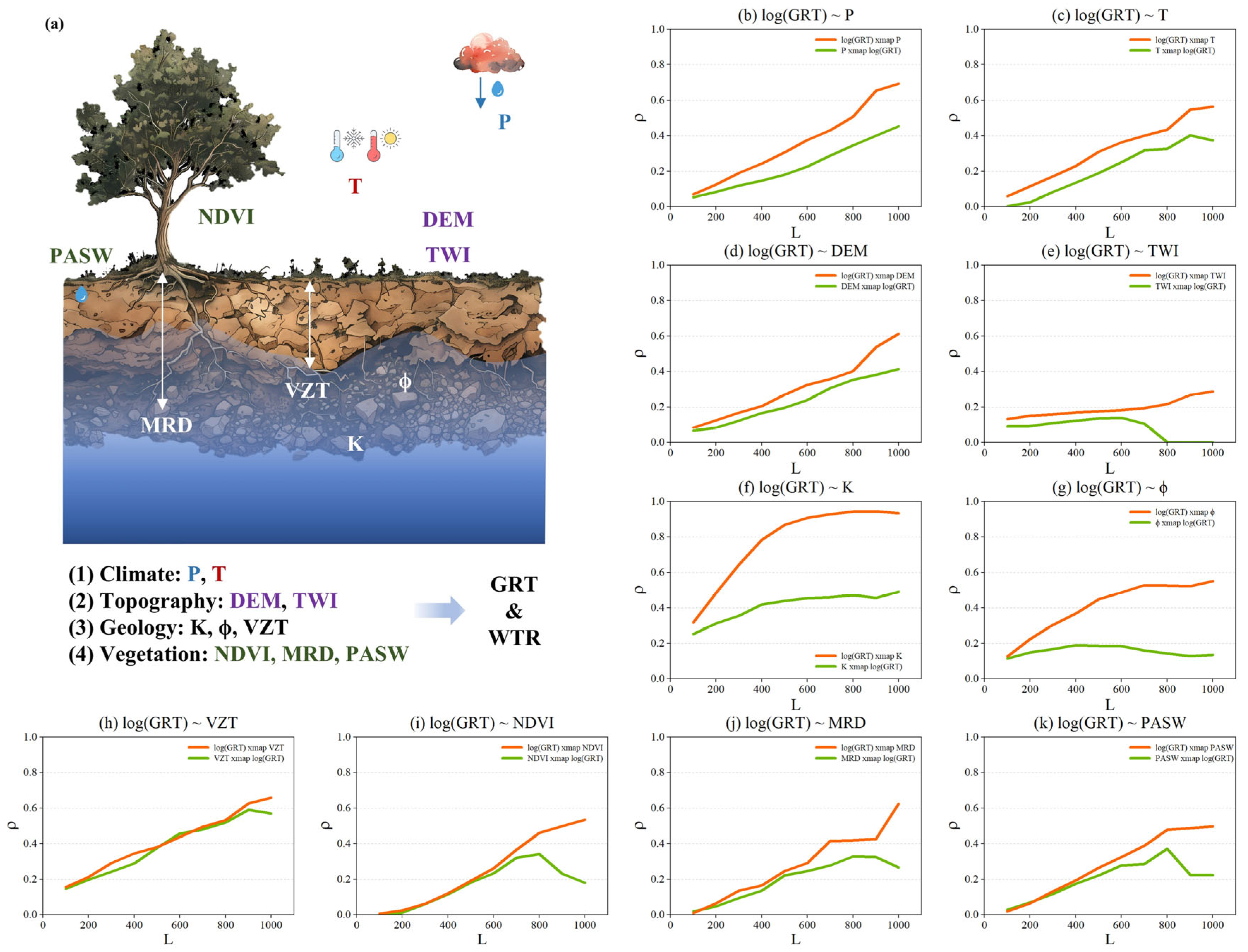
3.3. Causations Between GRT, WTR Type and Various Influencing Factors

The causations between GRT, WTR type, and multiple influencing factors were extracted by the GCCM. Figure 5a shows a concept map illustrating the factors influencing GRT and WTR. Climate-related factors included precipitation (P) and land surface temperature (T), while topographic influences were represented by the elevation (DEM) and Topographic Wetness Index (TWI). Geological factors comprised hydraulic conductivity (K), porosity (ϕ), and vadose zone thickness (VZT), and vegetation-related factors encompassed the Normalized Difference Vegetation Index (NDVI), Maximum Root Depth (MRD), and Potential Available Soil Water (PASW). Since the ultimate challenge for verifying causation models is the lack of observable evidence, the clear existence of causation between the 10 influencing factors and GRT (or WTR type) provides a valuable reference for assessing the reliability of causation models. Prior to analysis, the linear trends of the influencing factors and target variables (i.e., log-transformed GRT and WTR type) were removed to isolate the nonlinear interactions and better identify causal relationships. Due to limited space and similar causation outputs, here we mainly discuss the causation between GRT and influencing factors. The detailed method for linearity-removal is well-documented in [65]. Time consumption of the GCCM is shown in Supplementary Table S2.

As shown in Figure 5 and Supplementary Figure S1, the spatial distributions of GRT and its influencing factors exhibit distinct patterns, with limited similarity. Causal inference analyses, presented in Figure 5b–k, reveal that the reconstructed phase space of the 10 influencing factors and log(GRT) demonstrates a clearer spatial association after the GCCM process. This reconstruction shows the causal relationships between variables, particularly highlighting unidirectional causality between GRT and several factors, including the TWI, ϕ, NDVI, and PASW.

For example, the cross-mapping prediction skill (ρ) of log(GRT) xmap NDVI (noted as NDVI → GRT) is 0.53 (p  =  0.00), indicating a significant causal influence of NDVI on GRT. Similarly, causal relationships are observed for TWI → GRT (ρ = 0.29, p  =  0.05), ϕ → GRT (ρ = 0.55, p  =  0.00), and PASW → GRT (ρ = 0.50, p  =  0.00), all of which are relatively strong. Conversely, the reverse causality (e.g., GRT → NDVI, GRT → TWI) shows weaker and less significant correlations, with ρ values of 0.18 (p  =  0.00) and 0.00 (p  =  0.5), respectively.

GCCM causality analysis transcends correlation by quantifying driver-response directional dependence. It demonstrates K as the dominant GRT driver (ρ = 0.94), where conductivity perturbations propagate through aquifer networks to alter residence times. VZT (ρ = 0.85) and P (ρ = 0.78) are secondary controls, though their influence is nonlinear: <200 mm/yr precipitation yields negligible GRT changes, while >400 mm/yr induces exponential shortening (Figure 6b), revealing climate sensitivity thresholds.

Furthermore, P, T, DEM, K, and MRD exhibit large and significant causal influences on GRT distributions (ρ values ranging from 0.45 to 0.94). While GRT’s influence on these factors is still significant, the correlation is considerably smaller (ρ values ranging from 0.18 to 0.48). It is important to note that the significantly smaller ρ values for the reverse-direction cross-mapping (i.e., GRT → influencing factors) do not necessarily imply the existence of reverse causality [64,70]. Notably, a bidirectional causal relationship is observed between GRT and VZT. Collectively, the analysis reveals a hierarchy of causal influences: K, VZT, and P are dominant controls (ρ > 0.7), while T, DEM, and MRD show moderate effects (0.45 ≤ ρ ≤ 0.65). Other factors including ϕ, TWI, NDVI, and PASW demonstrate comparatively weaker causal linkages to GRT variability.

Crucially, GCCM exposes causal asymmetries missed by correlation analysis. While NDVI correlates moderately with GRT (r = 0.53), GCCM confirms unidirectional causality (NDVI → GRT: ρ = 0.53; GRT → NDVI: ρ = 0.18), indicating vegetation responds to groundwater accessibility rather than regulating it. Bidirectional causality between GRT-VZT (ρ = 0.85 in both directions) reflects their co-evolution: thick vadose zones prolong GRT, while slow groundwater flux enables chemical deposition that further reduces K. This systems perspective redefines “controls” as dynamic feedback loops rather than static factors.

3.4. Contributions of Influencing Factors

To quantify the contributions of each influencing factor to GRT and WTR type, we calculated and present these contributions in Figure 6. The GAM complements the findings from Section 3.3 by providing a numerical breakdown of the explanatory power of each factor. As shown in Figure 6a, the GAM accounts for 86.7% of GRT variation and 75.9% of WTR type variation. Specifically, the spatial variability of GRT is primarily driven by K, VZT, and P, which explain 34.3%, 13.5%, and 10.8% of the total contributions, respectively. In contrast, the variation in WTR type is largely influenced by VZT, TWI, and T, explaining 19.2%, 16.0%, and 9.6% of the contributions, respectively.

To explore the contributions of these significant factors further, we present the effect splines for each in Figure 6b–g. As illustrated in Figure 6b, P shows a slight increase and fluctuation in WTR type as it rises, while log(GRT) first decreases and then increases. In contrast, for K, Figure 6c reveals that both log(GRT) and WTR type decrease monotonically when K is below approximately 0.05 m/h, after which the values stabilize as K increases. The effect of TWI, shown in Figure 6e, indicates that when TWI is within the range of [−4, 5], there is minimal influence on the noise level of both log(GRT) and WTR type. However, as TWI increases beyond this range, the noise level in log(GRT) significantly increases. Figure 6f presents the effect of T, which follows a “U”-shaped curve, with both log(GRT) and WTR type decreasing initially before increasing. Notably, the response of WTR type is smoother than log(GRT), likely due to the smaller variability in WTR type. Significant differences are also observed in the GAM partial effect splines for VZT and NDVI, as shown in Figure 6d,g, reflecting their distinct mechanisms of influence on GRT and WTR type.

In summary, these findings indicate that the mechanisms through which P, VZT, T, and TWI influence the accuracy of both GRT and WTR type are distinct. In contrast, the influence of K on both GRT and WTR type follows a similar pattern.

4. Discussion

4.1. Limitations

Here, GRT and WTR maps are primarily derived from local lithological and hydrogeological data, providing an initial estimate of the response of unconfined groundwater systems across the global land surface. However, the more complex behaviors of regional or local confined aquifers, which may be critical for understanding groundwater–climate interactions, are not captured in this analysis. By employing analytical solutions to groundwater flow equations, we gain a significant advantage over more complex models, allowing for a direct analysis of the sensitivity of key parameters governing climate–groundwater interactions across the full parameter space, rather than relying on a restricted subset of parameters derived from numerical models. In addition, the accuracy of the input remote sensing data needs to be further improved.

While the statistical modeling framework employed in this study (GCCM/GAM) yields valuable insights into causal linkages within groundwater systems, we acknowledge inherent limitations associated with correlative approaches in capturing the full complexity of hydrological processes. In contrast to physically based models, which explicitly represent mechanistic interactions and flow dynamics, statistical methods are less adept at resolving nonlinear threshold responses, feedback loops, and hysteresis effects—particularly in confined aquifers where temporal lags and path-dependent stress propagation can obscure attribution. Moving forward, the integration of physically based models, such as coupled surface-subsurface simulations [32], should be prioritized to further resolve the emergent feedbacks identified through statistical approaches, particularly in transitional zones where water table behavior may exhibit threshold responses beyond the resolution of current empirical frameworks.

Our classification of water table types follows the globally established framework by Cuthbert et al. (2019) [51], where WTR > 1 defines topography-controlled systems and WTR < 1 defines recharge-controlled systems. As demonstrated in the global analysis [51], topography-controlled regimes (WTR > 1) exhibit shallow water tables (<10 m depth) and enable bidirectional groundwater-climate interactions: precipitation recharges aquifers, while groundwater directly supports evaporation/transpiration and modulates land-atmosphere energy fluxes. Conversely, recharge-controlled systems (WTR < 1) feature deeper water tables decoupled from topography, resulting in predominantly unidirectional interactions where climate influences groundwater, but feedback via ET is minimal. While lithological heterogeneity exists within HRB, our mapping (Figure 3c) aligns with the global paradigm: recharge dominance in arid lowlands (mid/lower basin) versus topographic control in humid/alpine zones (Qilian Mountains). This consistency validates our classification despite regional data constraints. Meanwhile, the WTR = 1 dichotomy effectively captures dominant interaction modes. However, intermediate values likely reflect hydrological gradients modulated by local vadose zone properties. This behavioral continuum agrees with the continental-scale framework which conceptualizes classification along a spectrum of water table connectivity [50]. Future high-resolution studies should quantitatively delineate these transition zones.

Locations where this approach may be less reliable tend to be in mountainous regions, where steep hillslope groundwater hydraulics may not be accurately represented. Consequently, our results may be less dependable in these areas. The GRT serves as an effective metric for long-term transience, an aspect currently difficult to model in state-of-the-art coupled groundwater-surface water models, which are constrained by their computational demands and limited to short run times even at the regional scale. More complex aquifer geometries and initial water table configurations lead to behaviors that diverge from simple exponential decay, with non-uniform flow fields (such as strong convergence or divergence) further influencing GRT variations [71,72,73].

Comparisons of WTR calculations with a more sophisticated 3D regional groundwater flow model suggest that WTR is a robust indicator of groundwater connectivity to the land surface [74]. It is a strong predictor of the dominance of local versus regional flow conditions [75]. This approach enables a large-scale estimate of the sensitivity of climate-groundwater interactions.

4.2. Implications of Complex Aquifer Behaviors in Climate-Groundwater Interactions

The intricate dynamics of confined aquifers, while not explicitly mapped in this study, play a pivotal role in modulating groundwater-climate feedbacks across the HRB. As demonstrated in global analogs like the Atacama Desert’s coastal aquifers [22], confined systems can exhibit decoupled response modes—where paleowater reserves (residence times > 10⁵ years) buffer short-term climate variations while remaining vulnerable to long-term depletion. Such systems often develop hydrological hysteresis, wherein aquifer responses lag climate forcing by centuries to millennia, creating “hidden vulnerabilities” that evade conventional monitoring [76]. In the HRB’s Quaternary foreland basins, seismic and borehole data suggest localized confined layers may explain anomalous GRT hotspots (e.g., Jiuquan Desert GRT > 10⁹ years), where low-permeability aquitards prolong hydraulic memory beyond topographically controlled systems. These behaviors necessitate specialized management strategies distinct from un-aquifer approaches.

Our GCCM-GAM framework offers a transferable pathway to address this complexity. By quantifying causal links between deep geological controls and GRT anomalies, the method identifies confinement signatures without requiring full 3D characterization—proving valuable in data-scarce regions. As implemented in the Locumba Basin [21], such attribution enables targeted geophysical surveys to verify predicted confined zones, optimizing limited resources.

Spatial causality further reveals hidden risks. Strong K → GRT causality (ρ = 0.94) but weak P → GRT links (ρ = 0.78) in confined systems indicate climate change impacts may manifest over centuries—a “hysteresis effect” requiring governance beyond electoral cycles. Integrating “Groundwaterscapes” [19] would contextualize these findings socio-ecologically, particularly where transboundary aquifers (e.g., Ejina Basin) face uncoordinated exploitation. Unlike global models assuming uniform sensitivity, our approach identifies “tipping zones” (e.g., alluvial fans with VZT < 10 m) where minor pumping could collapse desert spring ecosystems within decades.

4.3. Future Groundwater Conservation Proposal

Here we define the groundwater conservation area (GCA) as regions with a GRT of less than 100 years (called “human time-scale” in [51]). Figure 7 provides critical spatial context: Panel (a) visualizes aquifer recharge dynamics through GRT classification, revealing distinct temporal regimes across the basin, while Panel (b) explicitly overlays GCAs (GRT < 100 years) with existing protected zones to quantify conservation alignment gaps. This integrated analysis exposes a critical shortfall: only 6.72% of GCAs currently benefit from formal protection, leaving 93.28% of these climate-vulnerable aquifers exposed to unregulated anthropogenic stress. Although existing protected areas prioritize terrestrial biodiversity [77], we recommend strategic expansion into high-priority GCA zones (highlighted in Figure 7b) to safeguard groundwater-dependent ecosystems, particularly where spatial mismatches between recharge hotspots and protected boundaries threaten hydrological resilience in regions experiencing intensifying aridity.

5. Conclusions

Groundwater-climate interactions are inherently complex but crucial at the regional scale, with a comprehensive understanding of the underlying factors driving these interactions being essential for effective groundwater management. This study maps the spatial distributions of GRT and WTR using high-resolution remote sensing datasets and employs GCCM to explore causal relationships, alongside GAM to quantify the contributions of main influencing factors.

Through high-resolution mapping of GRT/WTR and causal attribution analysis, this work has achieved the following three primary objectives: (1) established basin-specific groundwater sensitivity thresholds using remote sensing proxies unavailable in global datasets; (2) demonstrated GCCM capability to extract causality from spatially complex systems where temporal analyses fail; and (3) quantified dominant controls (K, VZT, P for GRT; VZT, TWI, T for WTR) to prioritize conservation in vulnerable aquifers (<100-year GRT). These approaches provide a transferable framework for groundwater-climate studies in data-scarce arid regions.

Key findings include the following:

(1)

GRT distribution exhibits extreme temporal heterogeneity, with only 7.36% of the basin responding within 100 years while 85.23% exceeds 1000 years—including 71.91% > 10,000 years, confirming dominance of groundwater systems;

(2)

Water table types bifurcate along clear hydrogeological boundaries: recharge control predominates in shrublands/wetlands/croplands (WTR < 1), while topographic control prevails in forests/barelands (WTR > 1);

(3)

Climatic, topographic, geologic, and vegetative factors collectively explain 86.7% of GRT variance and 75.9% of WTR variability, with hydraulic conductivity (K), vadose zone thickness (VZT), and precipitation (P) identified as dominant GRT controls;

(4)

Spatial analysis reveals critical conservation gaps: merely 6.72% of vulnerable aquifers (GRT < 100 years) currently fall within protected areas;

(5)

The GRT-WTR synergy provides process-based interpretability—GRT contextualizes aquifer climate vulnerability while WTR identifies groundwater-mediated land-atmosphere coupling zones.

Collectively, the findings address three key knowledge gaps in groundwater science. First, the identification of basin-specific sensitivity thresholds provides unprecedented spatial granularity, exceeding that of current global-scale datasets. By incorporating the causal inference capabilities of the GCCM framework, the analysis overcomes inherent limitations of purely temporal assessments in complex and heterogeneous aquifer systems. Second, the quantified hierarchy of controlling factors offers a robust basis for spatial prioritization of recharge zones, particularly in arid lowland regions. Notably, the identification that 93.28% of aquifers with human-relevant response times (GRT < 100 years) remain outside existing protection frameworks highlights an urgent need for targeted policy interventions to mitigate risks of irreversible depletion. Third, the integration of GCCM, GAM, and remote sensing establishes a scalable and transferable methodological framework for groundwater vulnerability assessment in data-limited arid regions, effectively linking theoretical advances in hydroclimatic attribution with applied groundwater management strategies.

Future research should prioritize: (1) coupling statistical models with process-based simulations to validate inferred causal linkages, especially in confined aquifers; (2) expanding high-resolution observation networks in transitional hydrological zones characterized by near-unity water table ratios (WTR ≈ 1); and (3) designing adaptive conservation strategies for paleo-groundwater systems (GRT > 10,000 years), recognizing their non-renewable status and long-term role in regional hydroclimatic resilience. Advancing along these fronts will reinforce the integration of groundwater systems into climate adaptation frameworks, particularly within arid and endorheic basins.

References

1. Tanguy, M.; Chevuturi, A.; Marchant, B.P.; Mackay, J.D.; Parry, S.; Hannaford, J. How will climate change affect the spatial coherence of streamflow and groundwater droughts in Great Britain? Environ. Res. Lett. 2023, 18, 064048. [Google Scholar] [CrossRef]
2. Jaramillo, F.; Aminjafari, S.; Castellazzi, P.; Fleischmann, A.; Fluet Chouinard, E.; Hashemi, H.; Hubinger, C.; Martens, H.R.; Papa, F.; Schöne, T.; et al. The Potential of Hydrogeodesy to Address Water-Related and Sustainability Challenges. Water Resour. Res. 2024, 60, e2023WR037020. [Google Scholar] [CrossRef]
3. Mays, L.W. Groundwater Resources Sustainability: Past, Present, and Future. Water Resour. Manag. 2013, 27, 4409–4424. [Google Scholar] [CrossRef]
4. Scanlon, B.R.; Fakhreddine, S.; Rateb, A.; de Graaf, I.; Famiglietti, J.; Gleeson, T.; Grafton, R.Q.; Jobbagy, E.; Kebede, S.; Kolusu, S.R.; et al. Global water resources and the role of groundwater in a resilient water future. Nat. Rev. Earth Environ. 2023, 4, 87–101. [Google Scholar] [CrossRef]
5. Huang, B.; Zipper, S.; Peng, S.; Qiu, J. Groundwater effects on net primary productivity and soil organic carbon: A global analysis. Environ. Res. Lett. 2023, 18, 084024. [Google Scholar] [CrossRef]
6. Link, A.; El-Hokayem, L.; Usman, M.; Conrad, C.; Reinecke, R.; Berger, M.; Wada, Y.; Coroama, V.; Finkbeiner, M. Groundwater-dependent ecosystems at risk—global hotspot analysis and implications. Environ. Res. Lett. 2023, 18, 094026. [Google Scholar] [CrossRef]
7. Pandey, S.; Mohapatra, G.; Arora, R. Groundwater quality, human health risks and major driving factors in arid and semi-arid regions of Rajasthan, India. J. Clean. Prod. 2023, 427, 139149. [Google Scholar] [CrossRef]
8. Afkhami, S.; Massah Bavani, A.R.; Gohari, A.; Naderi, M.M.; Saadi, T. Sustainability analysis of single vs. multiple adaptation strategies in tackling the adverse impacts of climate change on groundwater resources using water-food-energy nexus approach. J. Clean. Prod. 2024, 459, 142532. [Google Scholar] [CrossRef]
9. de Graaf, I.E.M.; Marinelli, B.; Liu, S. Global analysis of groundwater pumping from increased river capture. Environ. Res. Lett. 2024, 19, 044064. [Google Scholar] [CrossRef]
10. Diodato, N.; Seim, A.; Ljungqvist, F.C.; Bellocchi, G. A millennium-long perspective on recent groundwater changes in the Iberian Peninsula. Commun. Earth Environ. 2024, 5, 257. [Google Scholar] [CrossRef]
11. Xie, J.; Liu, X.; Jasechko, S.; Berghuijs, W.R.; Wang, K.; Liu, C.; Reichstein, M.; Jung, M.; Koirala, S. Majority of global river flow sustained by groundwater. Nat. Geosci. 2024, 17, 770–777. [Google Scholar] [CrossRef]
12. Amanambu, A.C.; Obarein, O.A.; Mossa, J.; Li, L.; Ayeni, S.S.; Balogun, O.; Oyebamiji, A.; Ochege, F.U. Groundwater system and climate change: Present status and future considerations. J. Hydrol. 2020, 589, 125163. [Google Scholar] [CrossRef]
13. Tripathi, M.; Yadav, P.K.; Chahar, B.R.; Dietrich, P. A review on groundwater–surface water interaction highlighting the significance of streambed and aquifer properties on the exchanging flux. Environ. Earth Sci. 2021, 80, 604. [Google Scholar] [CrossRef]
14. Barthel, R.; Banzhaf, S. Groundwater and Surface Water Interaction at the Regional-scale—A Review with Focus on Regional Integrated Models. Water Resour. Manag. 2016, 30, 1–32. [Google Scholar] [CrossRef]
15. Lu, Z.; Peng, S.; Wu, T.; Lei, J.; Wei, J.; Yang, X. Effects of irrigation and canal networks on groundwater–land surface interactions in the middle Heihe River Basin, China. J. Hydrol. Reg. Stud. 2025, 60, 102532. [Google Scholar] [CrossRef]
16. Houspanossian, J.; Gimenez, R.; Whitworth-Hulse, J.I.; Nosetto, M.D.; Tych, W.; Atkinson, P.M.; Rufino, M.C.; Jobbagy, E.G. Agricultural expansion raises groundwater and increases flooding in the South American plains. Science 2023, 380, 1344–1348. [Google Scholar] [CrossRef]
17. Rohde, M.M.; Albano, C.M.; Huggins, X.; Klausmeyer, K.R.; Morton, C.; Sharman, A.; Zaveri, E.; Saito, L.; Freed, Z.; Howard, J.K.; et al. Groundwater-dependent ecosystem map exposes global dryland protection needs. Nature 2024, 632, 101–107. [Google Scholar] [CrossRef]
18. Rohde, M.M.; Stella, J.C.; Singer, M.B.; Roberts, D.A.; Caylor, K.K.; Albano, C.M. Establishing ecological thresholds and targets for groundwater management. Nat. Water 2024, 2, 312–323. [Google Scholar] [CrossRef]
19. Huggins, X.; Gleeson, T.; Villholth, K.G.; Rocha, J.C.; Famiglietti, J.S. Groundwaterscapes: A Global Classification and Mapping of Groundwater’s Large-Scale Socioeconomic, Ecological, and Earth System Functions. Water Resour. Res. 2024, 60, e2023WR036287. [Google Scholar] [CrossRef]
20. Huggins, X.; Gleeson, T.; Serrano, D.; Zipper, S.; Jehn, F.; Rohde, M.M.; Abell, R.; Vigerstol, K.; Hartmann, A. Overlooked risks and opportunities in groundwatersheds of the world’s protected areas. Nat. Sustain. 2023, 6, 855–864. [Google Scholar] [CrossRef]
21. Pocco, V.; Mendoza, A.; Chucuya, S.; Franco-León, P.; Huayna, G.; Ingol-Blanco, E.; Pino-Vargas, E. Assessment of Potential Aquifer Recharge Zones in the Locumba Basin, Arid Region of the Atacama Desert Using Integration of Two MCDM Methods: Fuzzy AHP and TOPSIS. Water 2024, 16, 2643. [Google Scholar] [CrossRef]
22. González-Domínguez, J.; Mora, A.; Chucuya, S.; Pino-Vargas, E.; Torres-Martínez, J.A.; Dueñas-Moreno, J.; Ramos-Fernández, L.; Kumar, M.; Mahlknecht, J. Hydraulic recharge and element dynamics during salinization in an overexploited coastal aquifer of the world’s driest zone: Atacama Desert. Sci. Total Environ. 2024, 954, 176204. [Google Scholar] [CrossRef] [PubMed]
23. Pino-Vargas, E.; Espinoza-Molina, J.; Chávarri-Velarde, E.; Quille-Mamani, J.; Ingol-Blanco, E. Impacts of Groundwater Management Policies in the Caplina Aquifer, Atacama Desert. Water 2023, 15, 2610. [Google Scholar] [CrossRef]
24. Yang, C.; Condon, L.E.; Maxwell, R.M. Unravelling groundwater–stream connections over the continental United States. Nat. Water 2025, 3, 70–79. [Google Scholar] [CrossRef]
25. Fan, Y.; Li, H.; Miguez-Macho, G. Global patterns of groundwater table depth. Science 2013, 339, 940–943. [Google Scholar] [CrossRef]
26. Reinecke, R.; Gnann, S.; Stein, L.; Bierkens, M.; de Graaf, I.; Gleeson, T.; Essink, G.O.; Sutanudjaja, E.H.; Ruz Vargas, C.; Verkaik, J.; et al. Uncertainty in model estimates of global groundwater depth. Environ. Res. Lett. 2024, 19, 114066. [Google Scholar] [CrossRef]
27. Ntona, M.M.; Busico, G.; Mastrocicco, M.; Kazakis, N. Modeling groundwater and surface water interaction: An overview of current status and future challenges. Sci. Total Environ. 2022, 846, 157355. [Google Scholar] [CrossRef]
28. Moyers, K.; Sabie, R.; Waring, E.; Preciado, J.; Naughton, C.C.; Harmon, T.; Safeeq, M.; Torres-Rua, A.; Fernald, A.; Viers, J.H. A Decade of Data-Driven Water Budgets: Synthesis and Bibliometric Review. Water Resour. Res. 2023, 59, e2022WR034310. [Google Scholar] [CrossRef]
29. Cai, P.; Li, R.; Guo, J.; Xiao, Z.; Fu, H.; Guo, T.; Wang, T.; Zhang, X.; Song, X. Spatiotemporal dynamics of groundwater in Henan Province, Central China and their driving factors. Ecol. Indic. 2024, 166, 112372. [Google Scholar] [CrossRef]
30. Irvine, D.J.; Singha, K.; Kurylyk, B.L.; Briggs, M.A.; Sebastian, Y.; Tait, D.R.; Helton, A.M. Groundwater-Surface water interactions research: Past trends and future directions. J. Hydrol. 2024, 644, 132061. [Google Scholar] [CrossRef]
31. Masciopinto, C.; Vurro, M.; Palmisano, V.N.; Liso, I.S. A Suitable Tool for Sustainable Groundwater Management. Water Resour. Manag. 2017, 31, 4133–4147. [Google Scholar] [CrossRef]
32. Lu, Z.; Wu, T.; Lei, J.; Yang, X. Assessing a high-resolution integrated hydrologic model (ParFlow-CLM-HRB) in an endorheic basin of China. J. Hydrol. 2025, 661, 133579. [Google Scholar] [CrossRef]
33. Li, X.; Cheng, G.; Lin, H.; Cai, X.; Fang, M.; Ge, Y.; Hu, X.; Chen, M.; Li, W. Watershed System Model: The Essentials to Model Complex Human-Nature System at the River Basin Scale. J. Geophys. Res. Atmos. 2018, 123, 3019–3034. [Google Scholar] [CrossRef]
34. Li, X.; Cheng, G.; Ge, Y.; Li, H.; Han, F.; Hu, X.; Tian, W.; Tian, Y.; Pan, X.; Nian, Y.; et al. Hydrological Cycle in the Heihe River Basin and Its Implication for Water Resource Management in Endorheic Basins. J. Geophys. Res. Atmos. 2018, 123, 890–914. [Google Scholar] [CrossRef]
35. Ge, Y.; Li, X.; Cheng, G.; Fu, B.; Liu, J.; Gao, L.; Zhong, F.; Zhang, L.; Wang, S. What dominates sustainability in endorheic regions? Sci. Bull. 2022, 67, 1636–1640. [Google Scholar] [CrossRef]
36. Yao, Y.; Tian, Y.; Andrews, C.; Li, X.; Zheng, Y.; Zheng, C. Role of Groundwater in the Dryland Ecohydrological System: A Case Study of the Heihe River Basin. J. Geophys. Res. Atmos. 2018, 123, 6760–6776. [Google Scholar] [CrossRef]
37. Yang, D.; Gao, B.; Jiao, Y.; Lei, H.; Zhang, Y.; Yang, H.; Cong, Z. A distributed scheme developed for eco-hydrological modeling in the upper Heihe River. Sci. China Earth Sci. 2015, 58, 36–45. [Google Scholar] [CrossRef]
38. Li, J.; Mao, X.; Li, M. Modeling hydrological processes in oasis of Heihe River Basin by landscape unit-based conceptual models integrated with FEFLOW and GIS. Agric. Water Manag. 2017, 179, 338–351. [Google Scholar] [CrossRef]
39. Lu, Z.; Wu, D.; Meng, S.; Kou, X.; Jiao, L. Exploration of Spatiotemporal Covariation in Vegetation–Groundwater Relationships: A Case Study in an Endorheic Inland River Basin. Land 2025, 14, 715. [Google Scholar] [CrossRef]
40. Li, X.; Cheng, G.; Liu, S.; Xiao, Q.; Ma, M.; Jin, R.; Che, T.; Liu, Q.; Wang, W.; Qi, Y.; et al. Heihe Watershed Allied Telemetry Experimental Research (HiWATER): Scientific Objectives and Experimental Design. Bull. Am. Meteorol. Soc. 2013, 94, 1145–1160. [Google Scholar] [CrossRef]
41. Li, X.; Cheng, G.; Fu, B.; Xia, J.; Zhang, L.; Yang, D.; Zheng, C.; Liu, S.; Li, X.; Song, C.; et al. Linking Critical Zone With Watershed Science: The Example of the Heihe River Basin. Earth’s Future 2022, 10, e2022EF002966. [Google Scholar] [CrossRef]
42. Lu, Z.; He, Y.; Peng, S. Assessing Integrated Hydrologic Model: From Benchmarking to Case Study in a Typical Arid and Semi-Arid Basin. Land 2023, 12, 697. [Google Scholar] [CrossRef]
43. Haitjema, H.M. On the residence time distribution in idealized groundwatersheds. J. Hydrol. 1995, 172, 127–146. [Google Scholar] [CrossRef]
44. Townley, L.R. The response of aquifers to periodic forcing. Adv. Water Resour. 1995, 18, 125–146. [Google Scholar] [CrossRef]
45. Erskine, A.D.; Papaioannou, A. The use of aquifer response rate in the assessment of groundwater resources. J. Hydrol. 1997, 202, 373–391. [Google Scholar] [CrossRef]
46. Zijl, W. Scale aspects of groundwater flow and transport systems. Hydrogeol. J. 1999, 7, 139–150. [Google Scholar] [CrossRef]
47. Haitjema, H.M.; Mitchell-Bruker, S. Are water tables a subdued replica of the topography? Groundwater 2005, 43, 781–786. [Google Scholar] [CrossRef]
48. Currell, M.; Gleeson, T.; Dahlhaus, P. A New Assessment Framework for Transience in Hydrogeological Systems. Groundwater 2016, 54, 4–14. [Google Scholar] [CrossRef]
49. Carr, E.J.; Simpson, M.J. Accurate and efficient calculation of response times for groundwater flow. J. Hydrol. 2018, 558, 470–481. [Google Scholar] [CrossRef]
50. Gleeson, T.; Marklund, L.; Smith, L.; Manning, A.H. Classifying the water table at regional to continental scales. Geophys. Res. Lett. 2011, 38, L5401. [Google Scholar] [CrossRef]
51. Cuthbert, M.O.; Gleeson, T.; Moosdorf, N.; Befus, K.M.; Schneider, A.; Hartmann, J.; Lehner, B. Global patterns and dynamics of climate–groundwater interactions. Nat. Clim. Chang. 2019, 9, 137–141. [Google Scholar] [CrossRef]
52. Liu, Z.; Feng, S.; Zhangsong, A.; Han, Y.; Cao, R. Long-term evolution of groundwater hydrochemistry and its influencing factors based on self-organizing map (SOM). Ecol. Indic. 2023, 154, 110697. [Google Scholar] [CrossRef]
53. Yang, R.; Mu, Z.; Gao, R.; Huang, M.; Zhao, S. Interactions between ecosystem services and their causal relationships with driving factors: A case study of the Tarim River Basin, China. Ecol. Indic. 2024, 169, 112810. [Google Scholar] [CrossRef]
54. Ehtiat, M.; Jamshid Mousavi, S.; Srinivasan, R. Groundwater Modeling Under Variable Operating Conditions Using SWAT, MODFLOW and MT3DMS: A Catchment Scale Approach to Water Resources Management. Water Resour. Manag. 2018, 32, 1631–1649. [Google Scholar] [CrossRef]
55. Lu, Z.; Chai, L.; Ye, Q.; Zhang, T. Reconstruction of Time-Series Soil Moisture from AMSR2 and SMOS Data by Using Recurrent Nonlinear Autoregressive Neural Networks. In Proceedings of the IEEE International Geoscience and Remote Sensing Symposium 2015 (IGARSS 2015), Milan, Italy, 26–31 July 2015. [Google Scholar]
56. Lu, Z.; Wei, J.; Yang, X. Effects of hydraulic conductivity on simulating groundwater–land surface interactions over a typical endorheic river basin. J. Hydrol. 2024, 638, 131542. [Google Scholar] [CrossRef]
57. Downing, R.A.; Oakes, D.B.; Wilkinson, W.B.; Wright, C.E. Regional development of groundwater resources in combination with surface water. J. Hydrol. 1974, 22, 155–177. [Google Scholar] [CrossRef]
58. Lu, Z.; Yang, X. Effects of microtopography on patterns and dynamics of groundwater–surface water interactions. Adv. Water Resour. 2024, 188, 104704. [Google Scholar] [CrossRef]
59. Berghuijs, W.R.; Luijendijk, E.; Moeck, C.; van der Velde, Y.; Allen, S.T. Global Recharge Data Set Indicates Strengthened Groundwater Connection to Surface Fluxes. Geophys. Res. Lett. 2022, 49, e2022GL099010. [Google Scholar] [CrossRef]
60. Gleeson, T.; Moosdorf, N.; Hartmann, J.; van Beek, L.P.H. A glimpse beneath earth’s surface: GLobal HYdrogeology MaPS (GLHYMPS) of permeability and porosity. Geophys. Res. Lett. 2014, 41, 3891–3898. [Google Scholar] [CrossRef]
61. Shangguan, W.; Hengl, T.; Mendes De Jesus, J.; Yuan, H.; Dai, Y. Mapping the global depth to bedrock for land surface modeling. J. Adv. Model. Earth Syst. 2017, 9, 65–88. [Google Scholar] [CrossRef]
62. Zhao, H.; Huang, W.; Xie, T.; Wu, X.; Xie, Y.; Feng, S.; Chen, F. Optimization and evaluation of a monthly air temperature and precipitation gridded dataset with a 0.025° spatial resolution in China during 1951–2011. Theor. Appl. Climatol. 2019, 138, 491–507. [Google Scholar] [CrossRef]
63. Zomer, R.J.; Xu, J.; Trabucco, A. Version 3 of the Global Aridity Index and Potential Evapotranspiration Database. Sci. Data 2022, 9, 409. [Google Scholar] [CrossRef]
64. Sugihara, G.; May, R.; Ye, H.; Hsieh, C.H.; Deyle, E.; Fogarty, M.; Munch, S. Detecting causality in complex ecosystems. Science 2012, 338, 496–500. [Google Scholar] [CrossRef]
65. Gao, B.; Yang, J.; Chen, Z.; Sugihara, G.; Li, M.; Stein, A.; Kwan, M.; Wang, J. Causal inference from cross-sectional earth system data with geographical convergent cross mapping. Nat. Commun. 2023, 14, 5875. [Google Scholar] [CrossRef]
66. Liu, J.; Chai, L.; Dong, J.; Zheng, D.; Wigneron, J.P.; Liu, S.; Zhou, J.; Xu, T.; Yang, S.; Song, Y.; et al. Uncertainty analysis of eleven multisource soil moisture products in the third pole environment based on the three-corned hat method. Remote Sens. Environ. 2021, 255, 112225. [Google Scholar] [CrossRef]
67. Wood, S.N.; Pya, N.; Säfken, B. Smoothing Parameter and Model Selection for General Smooth Models. J. Am. Stat. Assoc. 2016, 111, 1548–1563. [Google Scholar] [CrossRef]
68. Hu, Z.; Chai, L.; Crow, W.T.; Liu, S.; Zhu, Z.; Zhou, J.; Qu, Y.; Liu, J.; Yang, S.; Lu, Z. Applying a Wavelet Transform Technique to Optimize General Fitting Models for SM Analysis: A Case Study in Downscaling over the Qinghai–Tibet Plateau. Remote Sens. 2022, 14, 3063. [Google Scholar] [CrossRef]
69. Lu, Z.; He, Y.; Peng, S.; Yang, X. Comprehensive Evaluation of Multisource Soil Moisture Products in a Managed Agricultural Region: An Integrated Hydrologic Modeling Approach. IEEE J. Sel. Top. Appl. Earth Obs. Remote Sens. 2023, 16, 1–17. [Google Scholar] [CrossRef]
70. Stavroglou, S.K.; Pantelous, A.A.; Stanley, H.E.; Zuev, K.M. Hidden interactions in financial markets. Proc. Natl. Acad. Sci. USA 2019, 116, 10646–10651. [Google Scholar] [CrossRef]
71. Rousseau-Gueutin, P.; Love, A.J.; Vasseur, G.; Robinson, N.I.; Simmons, C.T.; de Marsily, G. Time to reach near-steady state in large aquifers. Water Resour. Res. 2013, 49, 6893–6908. [Google Scholar] [CrossRef]
72. Walker, G.R.; Gilfedder, M.; Dawes, W.R.; Rassam, D.W. Predicting Aquifer Response Time for Application in Catchment Modeling. Groundwater 2015, 53, 475–484. [Google Scholar] [CrossRef]
73. Cuthbert, M.O.; Acworth, R.I.; Andersen, M.S.; Larsen, J.R.; McCallum, A.M.; Rau, G.C.; Tellam, J.H. Understanding and quantifying focused, indirect groundwater recharge from ephemeral streams using water table fluctuations. Water Resour. Res. 2016, 52, 827–840. [Google Scholar] [CrossRef]
74. Gleeson, T.; Manning, A.H. Regional groundwater flow in mountainous terrain: Three-dimensional simulations of topographic and hydrogeologic controls. Water Resour. Res. 2008, 44, W10403. [Google Scholar] [CrossRef]
75. Condon, L.E.; Maxwell, R.M. Evaluating the relationship between topography and groundwater using outputs from a continental-scale integrated hydrology model. Water Resour. Res. 2015, 51, 6602–6621. [Google Scholar] [CrossRef]
76. Huggins, X.; Gleeson, T.; Castilla Rho, J.; Holley, C.; Re, V.; Famiglietti, J.S. Groundwater Connections and Sustainability in Social-Ecological Systems. Groundwater 2023, 61, 463–478. [Google Scholar] [CrossRef]
77. Luo, Q.; Li, S. Mapping human pressure in China and implications for biodiversity conservation. Ecol. Indic. 2024, 158, 111325. [Google Scholar] [CrossRef]
Figure 1. Maps of the study area: (a) location of the Heihe River Basin (HRB) and its surrounding areas; (b) DEM elevation over the HRB; (c) spatial patterns of climate classes; (d) spatial delineation of the lower (lHRB), middle (mHRB), and upper (uHRB) reaches as well as representative vegetation types over the HRB subregions (photo credit: Zheng Lu).
Remotesensing 17 02472 g001
Figure 2. Processing workflow of this study: brief explanations.
Remotesensing 17 02472 g002
Figure 3. The groundwater response times (GRT) and water table ratio (WTR) and their derived variables: (a) GRT expressed as log(GRT); (b) WTR expressed as log(WTR); (c) WTR types. Note that if WTR > 1, the area was of the “topography-controlled” type. Contrarily, WTR < 1 represents a “recharge-controlled” type where the groundwater system receives re-charge from the climate system. (d) porosity (S); (e) aquifer hydraulic conductivity (K); (f) aquifer thickness (H); (g) distance (L); (h) precipitation (P); (i) aridity (ϕ); (j) maximum terrain rise (d); (k) river distribution and traditional basin boundary maps over the Heihe River Basin (HRB).
Remotesensing 17 02472 g003
Figure 4. Groundwater response time (GRT) and water table ratio (WTR) over different landcovers: (a) landcover map over the HRB; (b) log(GRT) on different landcovers; (c) log(WTR) on different landcovers. Note that negative log(WTR) is recharge-controlled whereas positive log(WTR) is topography-controlled.
Remotesensing 17 02472 g004
Figure 5. Concept map showing influencing factors of groundwater response time (GRT), along with causal inference analyses for GRT. (a) Concept map illustrating causations between GRT and WTR and multiple influencing factors. All the Influences can be classified into four categories: climate, topography, geology and vegetation. (bk) Causal inference analyses for log(GRT). Climate-related factors include precipitation (P) and land surface temperature (T). Topographic influences are represented by the elevation (DEM) and Topographic Wetness Index (TWI). Geologic factors encompass hydraulic conductivity (K), porosity (ϕ), and vadose zone thickness (VZT). Vegetation-related factors include the Normalized Difference Vegetation Index (NDVI), Maximum Root Depth (MRD), and Potential Available Soil Water (PASW).
Remotesensing 17 02472 g005
Figure 6. Contributions of influencing factors: (a) contributions explained by variables related to log(GRT) and WTR type; (bg) partial effect splines from the generalized additive model (GAM) for precipitation (P), hydraulic conductivity (K), vadose zone thickness (VZT), temperature (T), and topographic wetness index (TWI), respectively. In panels (bf), the dotted lines represent the mean values for log(GRT) or WTR type (y-axis) and the explanatory variables (x-axis), while the shaded regions encompass the central 90% of the sample range. Additionally, small vertical lines at the bottom of each panel denote individual data points.
Remotesensing 17 02472 g006
Figure 7. Comparison of groundwater conservation priorities and zones of active groundwater renewal: (a) spatial classification of GRT classification map, highlighting temporal variability in aquifer recharge dynamics; (b) overlay of designated groundwater conservation areas with regions exhibiting GRT < 100 years, juxtaposed against the spatial extent of existing protected areas, illustrating alignment and potential mismatches between natural recharge zones and current management frameworks.
Remotesensing 17 02472 g007