Abstract
Detecting small objects in remote sensing images is challenging due to their size, which results in limited distinctive features. This limitation necessitates the effective use of contextual information for accurate identification. Many existing methods often struggle because they do not dynamically adjust the contextual scope based on the specific characteristics of each target. To address this issue and improve the detection performance of small objects (typically defined as objects with a bounding box area of less than 1024 pixels), we propose a novel backbone network called the Dynamic Context Branch Attention Network (DCBANet). We present the Dynamic Context Scale-Aware (DCSA) Block, which utilizes a multi-branch architecture to generate features with diverse receptive fields. Within each branch, a Context Adaptive Selection Module (CASM) dynamically weights information, allowing the model to focus on the most relevant context. To further enhance performance, we introduce an Efficient Branch Attention (EBA) module that adaptively reweights the parallel branches, prioritizing the most discriminative ones. Finally, to ensure computational efficiency, we design a Dual-Gated Feedforward Network (DGFFN), a lightweight yet powerful replacement for standard FFNs. Extensive experiments conducted on four public remote sensing datasets demonstrate that the DCBANet achieves impressive mAP@0.5 scores of 80.79% on DOTA, 89.17% on NWPU VHR-10, 80.27% on SIMD, and a remarkable 42.4% mAP@0.5:0.95 on the specialized small object benchmark AI-TOD. These results surpass RetinaNet, YOLOF, FCOS, Faster R-CNN, Dynamic R-CNN, SKNet, and Cascade R-CNN, highlighting its effectiveness in detecting small objects in remote sensing images. However, there remains potential for further improvement in multi-scale and weak target detection. Future work will integrate local and global context to enhance multi-scale object detection performance.
1. Introduction
Remote Sensing Object Detection (RSOD) focuses on accurately and efficiently identifying specific object classes within optical remote sensing images (RSIs) [1]. RSOD has long been a fundamental and challenging task. With the rapid advancements in deep learning, RSOD methods have made significant progress. For instance, novel frameworks have enhanced both accuracy and performance, including one-stage detectors like CFA [2] and RTMDet [3], and two-stage approaches such as RoI Transformer [4] and Oriented R-CNN [5].
However, remote sensing images contain a high prevalence of small objects. These objects are typically defined as having a bounding box area of fewer than 1024 pixels. Due to their limited size, these objects yield low-quality features, posing significant challenges for accurate recognition [6]. These small objects are susceptible to information loss during the convolution and pooling operations in neural networks. Furthermore, small objects are easily obscured by or confused with complex backgrounds, posing significant challenges for accurate localization and classification. Notably, for such objects, even slight perturbations in the bounding box can dramatically impact the Intersection over Union (IoU) metric, which in turn increases the learning difficulty for the regression branch.
To tackle the inherent difficulties in detecting small objects within RSIs, numerous advanced approaches have been developed [7]. These methods primarily employ strategies such as super-resolution reconstruction [8], multi-scale feature fusion [9,10], data augmentation [11], anchor optimization [12], and loss function refinement [13] to enhance the detection accuracy of small objects in RSIs. However, these methods still exhibit several critical limitations. While super-resolution modules can enhance the detailed features of small objects, they not only significantly increase computational complexity but may also degrade detection performance due to the generated artificial textures or edge artifacts. Multi-scale feature fusion methods that rely solely on simple concatenation or summation operations often suffer from feature incompatibility caused by the semantic gap between high-level and low-level features, leading to the suppression of crucial small object features by larger objects or background noise. Furthermore, other improvement strategies like anchor design optimization or loss function adjustments typically demonstrate only marginal gains in small object detection performance.
Recent studies [14,15] have demonstrated that contextual information plays a pivotal role in small object detection within remote sensing images. This is primarily because different categories of small objects may exhibit highly similar visual features, while environmental context can provide more discriminative feature representations for target identification [16]. In recent years, context-learning-based approaches for small object detection have emerged as a research focus, with a series of related works dedicated to exploring effective methods for leveraging scene context to enhance detection performance. YOLOX-CA [17] improves small object detection performance by incorporating convolutional kernels with varying dilation rates, effectively aggregating multi-scale contextual information to enhance the model’s sensitivity towards small targets. Li et al. [18] proposed a receptive field expansive deformable convolution that adaptively adjusts the context extraction scope and covers irregular contextual regions, thereby capturing appropriate contextual features to enhance the discriminability of small objects. DFCE [19] effectively detects small targets by integrating local and global contextual information and dynamically enhancing key features through a crossover mechanism.
Although existing context-learning-based methods have significantly improved the detection performance of small objects in remote sensing images, current approaches [20,21] still suffer from notable limitations. Primarily, most studies simply concatenate multi-scale contextual features without effectively highlighting crucial information. Furthermore, these methods fail to establish a truly adaptive context extraction mechanism, consequently limiting the model’s capability to dynamically adjust the utilization of contextual information based on target characteristics. To address these challenges, we propose a Dynamic Context Scale-Aware Block (DCSA Block) featuring multiple parallel branches that generate feature maps with varying receptive fields, coupled with a selective mechanism to adaptively determine the optimal contextual scope for each target. Furthermore, we introduce an Efficient Branch Attention (EBA) to dynamically reweight different branches, thereby enhancing those containing critical information. To compensate for the computational overhead induced by the multi-branch architecture, we devise a Dual-Gated Feedforward Network (DGFFN) that significantly reduces both parameters and computational complexity while improving inference efficiency. The main contributions of this work are threefold:
- We propose a DCSA Block with a multi-branch architecture, which can adaptively capture the optimal range of contextual information for small objects in RSIs. Furthermore, we introduce an EBA module that employs dynamic weight adjustment to significantly enhance the network’s capability to utilize branches containing critical information.
- We propose a DGFFN that effectively reduces the number of parameters and complexity while improving the detection speed of the model by introducing gating mechanisms into the feedforward network.
- We construct a novel lightweight backbone network called the Dynamic Context Branch Attention Network (DCBANet) by repeatedly stacking the proposed components. The network demonstrates outstanding performance on public remote sensing datasets, validating that our components effectively and dynamically adapt to small targets of various sizes. This highlights the model’s universal applicability in detecting small objects across the entire scale range (<1024 pixels).
2. Related Works
2.1. RSOD Frameworks
RSOD frameworks based on deep learning can be categorized into one-stage methods and two-stage methods. One-stage methods, such as R3Det [22] and S2A-Net [23], demonstrate superior computational efficiency and real-time processing capabilities by directly predicting the bounding box, class, and confidence of the objects in the input image, albeit with relatively lower detection accuracy. In contrast, two-stage methods, exemplified by advanced frameworks like Cascade R-CNN [24] and Dynamic R-CNN [25], are based on the classical Regional Convolutional Neural Network [26] (RCNN) architecture, which first generates region proposals and subsequently performs a more fine-grained object categorization and bounding box regression on these proposals. Therefore, they have a distinct advantage in terms of object detection accuracy. Inspired by the DETR [27] model, some recent studies [28,29] have proposed end-to-end oriented detectors, which effectively resolve the inconsistency between object classification and localization in traditional models.
While these one-stage and two-stage frameworks have achieved remarkable success, their direct application to small object detection in RSIs is often sub-optimal. The core challenge stems from the feature representation of small objects. The hierarchical structure of deep networks, with its repeated down-sampling operations, inherently leads to the loss of crucial high-resolution spatial information. This makes it exceedingly difficult for subsequent detection heads to accurately localize and classify tiny targets, regardless of whether they are anchor-based or anchor-free. Therefore, designing a backbone network that can effectively preserve and enhance discriminative features for small objects is of paramount importance.
2.2. Small Object Detection
In recent years, small object detection has emerged as a prominent research direction in the field of computer vision. QueryDet [30] proposed a detector based on coarse location queries. The method first predicts regions in the image where small objects may exist and then utilizes high-resolution features in these specific regions for object localization and classification. EFPN [31] introduces a super-resolution module into the traditional feature pyramid network to apply super-resolution operations only to small-sized feature maps. It improves detail representation for small objects, but at the expense of increased computational effort and model complexity. ABFPN [32] expands the receptive field of the feature maps by employing skip-ASPP blocks with varying dilation rates and applies jump-joining to adequately fuse the multi-scale features, which effectively avoids the problem of potentially weakening the semantic information when performing lateral joining. ABNet [33] proposed an adaptive FPN capable of dynamically extracting multi-scale features across different channels and spatial locations. SCRDet++ [34] applies an instance-level denoising method to small object detection for the first time and improves the Smooth-L1 loss function to address challenges in boundary detection.
In summary, existing small object detection methods primarily focus on strategies like multi-scale feature fusion, super-resolution, and context enhancement. However, many context-based approaches simply aggregate contextual information without a mechanism to dynamically adapt the context range based on the target’s specific characteristics. This static context aggregation can be sub-optimal, as different small objects may require different contextual cues for accurate identification. This gap motivates our work on a dynamic context-aware module.
2.3. Attention Mechanisms
Attention mechanisms [35] have become a powerful tool for enhancing feature representation in computer vision, and they are particularly relevant for small object detection. By allowing the model to focus on the most informative features, attention can help distinguish tiny objects from a cluttered background. [36]. SENet [37] uses global average pooling to capture global information, followed by fully connected and activation layers in the excitation module to capture channel relationships to output channel weights. ECANet [38] considers only local cross-channel interactions, where each channel interacts with its K-nearest neighboring channels rather than capturing all inter-channel relationships, while using 1 × 1 convolution instead of fully connected layers to generate channel weights. GENet [39] captures the broader context by aggregating feature responses from spatial neighborhoods and then redistributes the aggregated information to local features to adjust the original feature responses, ultimately yielding a spatial attention map. PSANet [40] proposes a point-wise spatial attention that achieves the aggregation of long-range contextual information by learning the correlation between each pixel pair and thus enabling the dynamic adjustment of weights between them. ViT [41] splits the image into small patches and employs a self-attention mechanism to learn inter-region relationships, which can better aggregate the image’s global context. ResNeSt [42] enhances the model’s feature representation capability by incorporating multiple branches into the ResNet architecture and introduces a new attention mechanism, Split-Attention, which can dynamically adjust the weights of different branches.
However, most channel attention mechanisms like SENet or ECANet treat all branches or feature groups equally or competitively, which may not be ideal for our multi-branch architecture, where different branches capture distinct types of contextual information. A mechanism that can independently weight and preserve critical information from each branch is therefore desirable for our specific task of small object detection.
2.4. Feedforward Network
Feedforward networks (FFNs) are an important part of transformer models [41,43] and are primarily composed of a multilayer perceptron (MLP). The MLP enhances the feature representation by a series of linear transformations and nonlinear activation functions. However, the parameters in the MLP account for more than 60% of the entire model, making it the main source of the computational bottleneck issue. To address this problem, SparseFFN [44] reduces the parameters of the FFN through channel-wise sparsification using grouped linear layers and spatial-wise sparsification via feature pooling to capture regional semantics. Compact FFN [45] factorizes the projection matrix at the second linear layer to reduce redundancy and further compresses the FFN using reparameterization techniques. Some studies have focused on leveraging gating mechanisms [46] to simplify FFNs, as these mechanisms are capable of controlling which information should be retained, enhanced, or discarded. MAN [47] introduces simple spatial attention in a linear gating unit to remove unnecessary linear layers, thus drastically reducing the number of parameters in the FFN. MogaNet [48] reduces the large number of redundant features caused by conventional FFNs by introducing a channel aggregation module based on gating mechanisms to redistribute the multi-order features in the feedforward network. Although these methods reduce the number of parameters in the FFN, they also lead to a reduction in the model’s overall performance.
While these methods successfully reduce the parameters and complexity of the FFN, they often do so at the cost of performance, which can be detrimental for the already challenging task of small object detection, where every bit of feature representation capability matters. Therefore, designing a lightweight FFN that minimizes performance degradation is a key challenge. This motivates our proposed Dual-Gated Feedforward Network (DGFFN), which aims to strike a better balance between efficiency and accuracy, a critical consideration for deploying detectors on large-scale remote sensing data.
3. Method
3.1. DCBANet Backbone Architecture
As shown in Figure 1, the overall architecture of our proposed DCBANet backbone network adopts a multi-stage design, where each stage outputs a feature map of different sizes. DCBANet is inspired by LSKNet [14], ECANet [38], ResNeSt [42], GCT [46], MAN [47], and VAN [49].
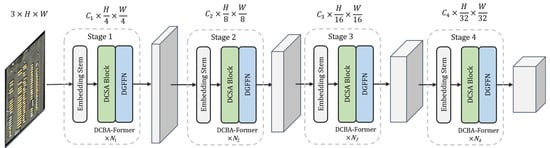
Figure 1.
The overall architecture of the DCBANet backbone network. It is divided into four stages, each of which consists of a series of serially stacked DCBA-Formers. The embedding dimensions at each stage are set to {64, 128, 320, 512}, and the number of DCBA-Formers. is configured as {2, 2, 4, 2}.
Each stage in the backbone network consists of a repetitive stack of DCBA-Former based on the MetaFormer [50] architecture. As illustrated in Figure 2, each DCBA-Former comprises a DCSA residual sub-block and a DGFFN residual sub-block. The DCSA sub-block serves to dynamically extract spatial context information for small objects. The DGFFN sub-block primarily functions to enhance the feature representation at each location and introduce nonlinearity.
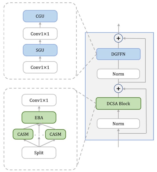
Figure 2.
The structure of a DCBA-Former.
3.2. Dynamic Context Scale-Aware Block
To enable adaptive adjustment of contextual information, we propose the DCSA Block (illustrated in Figure 3). It is a block-level multi-branch design, which differs from conventional network-level multi-scale feature extraction. While traditional multi-scale approaches generate feature maps of different spatial resolutions at different stages of the network to handle variations in object size, our DCSA Block operates on a single feature map from a specific stage. It incorporates a multi-branch architecture with varying kernel sizes to generate feature maps with diverse receptive fields at the same scale and resolution. A selective mechanism is then employed to dynamically choose the most appropriate contextual range for each target. This approach is particularly effective for small objects, as their recognition often depends on fine-grained local context rather than broad semantic information from different scales. This design effectively overcomes the limitation of fixed contextual ranges inherent to single-kernel approaches.
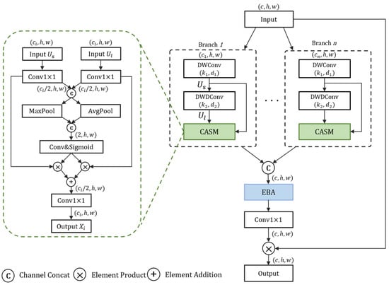
Figure 3.
The architecture of the proposed DCSA Block. It consists of multiple parallel branches to generate features with diverse receptive fields. Each branch contains a Context Adaptive Selection Module (CASM), shown in detail on the left, which dynamically weights features from smaller () and larger () receptive fields. The outputs from all branches are subsequently processed by an EBA. The detailed structure of the EBA is depicted in Figure 4.
Specifically, given an input image , we divide it into multiple parts in terms of channel dimensions. These parts are then processed by distinct branches, each employing a different large convolution kernel. To mitigate the substantial parameter overhead induced by large convolutional kernels, we decompose each of them into two smaller depthwise convolutional kernels. This decomposition process can be formulated as follows:
where denotes a large convolution kernel; denotes a 1 × 1 convolution; denotes a depthwise convolution with a kernel size of ; and denotes a depthwise dilated convolution with a kernel size of and a dilation rate of . The input in each branch sequentially undergoes both a depthwise convolution and a depthwise dilated convolution to generate two feature maps with distinct receptive fields: one with a smaller receptive field (defined as ) and the other with a larger one (defined as ):
and are first compressed along the channel dimension to reduce redundant features and then concatenated. The combined feature map is subsequently subjected to average pooling and maximum pooling to extract spatial relationships. The pooled feature map is defined as :
where and denote average pooling and maximum pooling operations, respectively. To extract appropriate context information for different objects in and , the weights of different regions are first calculated:
where represents the activation function and denotes the spatial weight coefficient with two channels (defined as and ). Weighting and fusing the weight coefficients with the corresponding feature maps realize the selection of appropriate contextual information for small objects. denotes the final obtained spatial feature map:
3.3. Efficient Branch Attention
To highlight critical branches and enhance the utilization of discriminative features, we introduce an Effective Branch Attention (EBA) module that dynamically adjusts branch-wise weights. The key innovation lies in employing 1 × 1 convolutions (instead of fully connected layers) to generate channel-wise weights, which effectively prevents information loss during channel compression while reducing parameter overhead. Furthermore, the application of sigmoid activation to channel weights ensures more stable training dynamics. Notably, the sigmoid activation allows each channel weight to be activated independently without competition among branches, thereby better preserving discriminative feature representations. Specific details are shown in Figure 4.
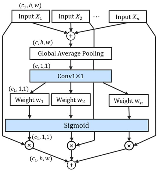
Figure 4.
The flowchart of the EBA module. denotes the number of channels in the feature maps of each branch. represents the total number of channels across all branches.
First, we concatenate the results obtained from all branches along the channel dimension to obtain , which is assumed to have the shape of :
where is the result of different branches and is the number of branches. Then, a global average pooling operation is applied to it:
where represents the value located at spatial coordinates within the -th feature map , while corresponds to the aggregated channel-wise descriptor for the -th channel. The pooled feature vector thus consists of elements, corresponding to the number of channels in . Subsequently, we employ a lightweight 1 × 1 convolution to generate channel-wise weights, which are then activated via a sigmoid function:
where denotes the sigmoid activation function. In contrast, Split Attention [42] employs softmax activation, which creates zero-sum competition among branches and can potentially lead to the loss of effective features. Conversely, the sigmoid function permits independent multi-channel activation, unaffected by other branches, thereby enabling more effective feature fusion. The final output of EBA is computed as a weighted sum of the input branches:
In the final step, a 1 × 1 convolution is applied to . The result is then added to the original input through a residual connection to produce the final output of the DCSA Block:
The algorithmic details of the DCSA Block are summarized in Algorithm 1.
| Algorithm 1: Forward Propagation Process of the DCSA Block |
| Input: Feature map X_in |
| Output: Feature map X_out |
| 1: Split X_in into n branches: X_1, X_2, …, X_n |
| 2: Initialize an empty list of branch outputs: Outputs = [] |
| 3: for i = 1 to n do |
| 4: //Decomposed large kernel convolution |
| 5: U_s_i = Conv1×1(DWConv_k1(X_i)) |
| 6: U_l_i = Conv1×1(DWDConv_k2,d(U_s_i)) |
| 7: //Context Adaptive Selection Module (CASM) |
| 8: U_combined_i = Concat(Conv1×1(U_s_i), Conv1×1(U_l_i)) |
| 9: W_i = σ(Conv1×1(Concat(P_avg(U_combined_i), P_max(U_combined_i)))) |
| 10: X_branch_out_i = W_s_i × U_s_i + W_l_i × U_l_i |
| 11: Append X_branch_out_i to Outputs |
| 12: end for |
| 13://Efficient Branch Attention (EBA) |
| 14: X_cat = Concat(Outputs) |
| 15: Y_pooled = GlobalAvgPool(X_cat) |
| 16: w_eba = σ(Conv1 × 1(Y_pooled)) |
| 17: X_eba = Σ (w_eba_i × X_branch_out_i) |
| 18://Residual Connection |
| 19: X_out = Conv1×1(X_eba) + X_in |
| 20: return X_out |
3.4. Dual-Gated Feedforward Network
The MLP typically maps input features to hidden features with 4× or 8× higher dimensions, leading to a substantial parameter count in the fully connected layers [44]. Directly reducing the hidden feature dimensions or performing grouping operations may drastically reduce model performance. To reduce parameters while maintaining superior performance, we design a gating mechanism-based feedforward network named the Dual-Gated Feedforward Network (DGFFN).
The DGFFN (Figure 5) comprises two components: a Spatial Gating Unit (SGU) and a Channel Gating Unit (CGU). The SGU enhances local feature representation by generating spatial gating weights. The CGU introduces three learnable parameters to enhance its contextual information modeling capability by adjusting the competitive and complementary relationships between channels.
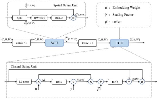
Figure 5.
The structure of the Dual-Gated FFN. The SGU and CGU based on gating mechanisms are introduced into the traditional MLP.
In the DGFFN, the input tensor is assumed to be , and the hidden layer expansion ratio is . The input features are first extended to the high-dimensional hidden feature tensor via a 1 × 1 convolution, which is in line with the traditional MLP.
Spatial Gating Unit (SGU). The SGU is built on the basis of a gated linear unit, which receives the high-dimensional hidden feature from the previous step as input, and then divides it equally into two parts along the channel dimension:
where is the gating feature used to generate the gating weights and is the other feature part, which undergoes the subsequent weighting operation. At this point, the channel dimension of both parts is . The gating feature is transformed into gating weights via a depthwise convolution. The gating weights are then element-wise multiplied by the feature part to implement the gating effect:
where is the feature after spatial gating with the same channel dimension . After the SGU, the channel dimension is again restored to via 1 × 1 convolution.
Channel Gating Unit (CGU). In the CGU, three learnable parameters , , and are introduced, where is used to control the scaling factor of the feature channel, controls the offset of the gating value, and controls the channel normalization.
First, for the input , compute a spatial embedding for each channel using its L2-norm scaled by a learnable parameter:
where is the feature value at spatial coordinates of the -th channel; indicates a small constant added to prevent numerical instability; and is a learnable parameter used to scale the embedding values. The resulting value represents the scaled spatial intensity of each channel. Next, each channel is normalized:
where denotes the root mean square value; is the number of channels; and denotes a learnable scaling factor that modulates the gating strength of each channel by controlling the degree of channel normalization. The gating factor is then calculated as
where represents a bias and refers to the hyperbolic tangent function. This function first compresses the input value to , and the addition of the constant 1 subsequently adjusts the range to , yielding a suitable gating value for weighting. Finally, the gated weighting operation is performed via element-wise multiplication:
The DGFFN primarily reduces the computational complexity by decreasing the input channel dimensions of the subsequent depthwise convolutional layer and the second linear (e.g., 1 × 1 convolutional) layer, enabled by the split operation in the SGU. Since the CGU does not involve computationally intensive convolution or fully connected operations, its computational complexity is generally considered negligible. The DGFFN can replace the feedforward networks in various transformer models to achieve model lightweighting while enhancing performance.
4. Experiments
4.1. Datasets
DOTA [51] is a leading benchmark dataset in remote sensing image analysis, consisting of 2806 high-resolution aerial images. The dataset is split into training, validation, and test sets at a 1411:458:937 ratio. Image resolutions range from 800 × 800 to 4000 × 4000 pixels, highlighting significant multi-scale properties. This dataset includes 15 common classes annotated with oriented bounding boxes (OBBs), with a total of 188,282 annotated instances. The average width of these instances is 27.60 pixels, with approximately 60% of instances measuring less than 20 pixels in width.
NWPU VHR-10 [52] is a dataset comprising 650 remote sensing images with very high resolutions. The images feature spatial resolutions between 0.5 m and 2 m and pixel dimensions varying between 533 × 597 and 1728 × 1028. The dataset is annotated with 10 object categories, totaling 3651 annotated instances. For this study, we apply a random split approach to partition the dataset into training and test sets equally, resulting in 325 images allocated to training and 325 images to testing.
SIMD [53] is a specialized remote sensing dataset for detecting vehicles and aircrafts. It contains 5000 images at a resolution of 1024 × 768 pixels, divided into 4000 for training and 1000 for testing. It covers 15 object categories, which the original authors classified into three groups based on object scale characteristics: small-scale objects (including Cars, Vans, Stair Trucks, Pushback Trucks, Others, Boats, and Helicopters); medium-scale objects (including Trucks, Buses, Trainer Aircrafts, and Fighter Aircrafts); and large-scale objects (including Long Vehicles, Airliners, Propeller Aircrafts, and Chartered Aircrafts). Among these, small-scale targets account for over 80% of the total instances.
AI-TOD [54] is a dataset specifically constructed for remote sensing small target detection, which contains 28,036 remote sensing images with 800 × 800 pixels. The dataset contains 700,621 annotated object instances across eight categories. Notably, the average object size is merely 12.8 pixels, which is significantly smaller than in other datasets. This characteristic makes AI-TOD particularly challenging for evaluating the performance of small object detection models.
The AI-TOD dataset further divides small objects (<1024 pixels) into three scale ranges based on the area of the bounding box: generally small (256–1024 pixels), tiny (64–256 pixels), and very tiny (8–64 pixels). According to this classification criterion, Figure 6 shows the scale distribution of small- and medium-sized objects in DOTA, NWPU VHR-10, SIMD, and AI-TOD. Both DOTA and AI-TOD contain many small objects, especially AI-TOD, which contains 255,227 tiny objects and 43,519 very tiny objects.
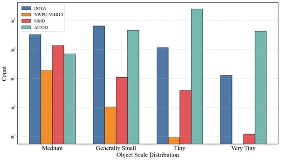
Figure 6.
Distribution of object scales in the DOTA, SIMD, NWPU VHR-10, and AI-TOD datasets. The scales are categorized as: normal (1000–4096 pixels), general small (256–1024 pixels), tiny (64–256 pixels), and very tiny (4–64 pixels).
4.2. Experimental Setup and Evaluation Metrics
4.2.1. Experimental Setup
For our experiments, we integrated the proposed DCBANet backbone into the MMDetection framework (version 3.3.0). We consistently used a standard Feature Pyramid Network (FPN) as the neck. For the detection head, unless otherwise specified, the default detectors used in the experiment are Faster-RCNN (HBB task) or Oriented-RCNN (OBB task).
Our proposed method was implemented using the PyTorch framework (version 1.10.0), and the experiments were carried out on an NVIDIA RTX 4090 GPU with 24 GB (NVIDIA Corporation; Santa Clara, CA, USA) of memory. We employed the AdamW optimizer for network optimization, with hyperparameters including an initial learning rate of , a weight decay coefficient of 0.05, and beta parameters set to (0.9, 0.999). During the inference phase, the key parameters were set as follows: the maximum number of proposals was limited to 2000, the confidence threshold was 0.05, and the IoU threshold for Non-Maximum Suppression (NMS) was 0.5. For consistent calculation of model complexity, the input tensor size was fixed at (1, 3, 1024, 1024) when calculating the parameter count (Param) and Floating-point Operations (FLOPs).
For the DOTA dataset, during single-scale training, the original images were cropped into 1024 × 1024-pixel patches with a stride of 824 pixels and a 200-pixel overlap. During multi-scale training, the images were resized with scaling factors of 0.5, 1.0, and 1.5, followed by cropping with a stride of 524 pixels and a 500-pixel overlap. The batch size was set to 2 during training. Consistent with mainstream practices, the model was trained using both the training and validation sets, and the final test results were generated through the official DOTA evaluation server.
For the SIMD, NWPU VHR-10, and AI-TOD datasets, we standardized the resolution of the original images to 1024 × 1024 pixels for both training and testing. Random flipping was applied as a data augmentation strategy, and the batch size was set to 4.
4.2.2. Evaluation Metrics
This study employs Average Precision (AP) and mean Average Precision (mAP) to evaluate detection accuracy, Frames Per Second (FPS) to measure detection speed, and Floating-point Operations (FLOPs) to assess computational complexity.
AP measures the overall performance of the model at different confidence thresholds by calculating the area under the Precision–Recall curve. By default, the Intersection over Union (IoU) threshold is 0.5. The calculation formula is as follows:
where P (Precision) represents the proportion of samples predicted by the model to be positive that are actually positive, and R (Recall) represents the proportion of positive samples correctly detected by the model out of all actual positive samples.
The calculation of mAP involves first computing the AP for each category and then taking the average of the AP values across all categories:
where stands for the total number of object categories.
When conducting experiments on the AI-TOD dataset, we evaluate our results based on the COCO benchmark. The evaluation relies on the Average Precision (AP) metric, where the primary metric, mAP@0.5:0.95, is calculated by averaging AP values over ten IoU thresholds from 0.5 to 0.95, providing a comprehensive assessment of localization accuracy. We also report mAP@0.5 (IoU = 0.5) and mAP@0.75 (IoU = 0.75). Furthermore, to analyze performance across different object sizes, we utilize , , and , which correspond to mAP@0.5:0.95 for small (<1024 pixels), medium (1024–9216 pixels), and large (>9216 pixels) objects. Given the abundance of small targets in AI-TOD, the metric is particularly critical for our analysis.
4.3. Ablation Study
Ablation Study on Branch Number and Large Kernel Decomposition Sequences. In the DCSA Block, different large kernel decomposition sequences generate feature maps with varying receptive fields, which directly influence subsequent context-adaptive performance. Meanwhile, the number of branches significantly impacts the model’s detection speed. A well-designed combination of branch numbers and large kernel decomposition sequences can achieve an optimal trade-off between speed and accuracy. LSKNet [14] was selected to be the baseline model. We replaced its LK Selection module with the multi-branch-based DCSA Block and evaluated the performance of different branch numbers and large kernel decomposition sequences. The selection of kernel decomposition sequences is guided by the following principles:
1. Diverse Receptive Fields Coverage: The primary objective is to cover a wide spectrum of receptive fields. A larger RF, achieved through larger kernels () or dilation rates (), enables the model to capture broader contextual cues, which are vital for distinguishing small objects from complex backgrounds. A smaller receptive field focuses on fine-grained local details.
2. Computational Efficiency: Our decomposition strategy, breaking a large kernel into two smaller depthwise convolutions (e.g., (, ) and (, )), significantly reduces the parameter count and computational load compared to a single large dense kernel. The choice of and is kept small (e.g., 3, 5, 7) to maintain this efficiency.
3. Avoiding Gridding Artifacts: While a large dilation rate d can rapidly expand the RF, it can also lead to the “gridding effect [47],” where the convolution kernel samples the input feature map sparsely, potentially missing important local information. Our sequential decomposition mitigates this by combining a standard convolution ( = 1) with a dilated one, ensuring both dense local coverage and expanded contextual view.
As shown in Table 1, when using a three-branch configuration, the sequence producing RFs of {15, 23, 31} (derived from kernel sequences {(3, 1), (7, 2)}, {(5, 1), (7, 3)}, and {(7, 1), (9, 3)}) yielded the best mAP of 75.05%. This configuration provides a balanced and well-spaced distribution of receptive fields, covering small, medium, and large contextual areas without significant overlap. In contrast, increasing the number of branches to four (e.g., with RFs {15, 23, 29, 39}) did not lead to further improvement and decreased the inference speed (FPS), suggesting that three distinct contextual ranges are sufficient for this task and additional branches may introduce redundancy. The baseline model, with a single RF of 23, lacks this flexibility, resulting in a lower mAP of 74.72%. This confirms that our multi-branch decomposition strategy, guided by the principles above, is effective at enhancing feature extraction capabilities in an efficient manner.

Table 1.
Branch number and large kernel decomposition sequence partial configurations and results, where RF denotes large kernel receptive fields, denotes the convolution kernel, and denotes dilation rate. Experiments were conducted on the DOTA dataset with a training schedule of 3×. The initial weights of all models in this experiment were randomly initialized.
Ablation study on the impact of DGFFN on parameter count, complexity, and performance. To assess the efficacy and robustness of the introduced DGFFN module, ablation studies were performed across three distinct backbones: LSKNet [14], Swin-t [43], and DCBANet (Ours). Table 2 shows the number of parameters, FLOPs, mAP, and FPS for models incorporating either the standard MLP or the proposed DGFFN within these backbone networks. Additionally, we also evaluate the performance of GSAU [47] and CAFFN [48], which are based on gating mechanisms.
Table 2.
Performance comparison between standard MLP and DGFFN. The proposed DGFFN reduces both parameters (Param) and FLOPs while improving detection performance (mAP) and inference speed (FPS) across all architectures. Experiments were conducted on the DOTA dataset with a training schedule of 3×. The initial weights of all models in this experiment were randomly initialized. ‘↑’ and ‘↓’ indicate the rise or fall of each metric, respectively.
The experimental results clearly demonstrate the lightweight advantages of our proposed DGFFN across various backbone architectures. Specifically, when integrated into LSKNet, DGFFN reduces the parameter count by 15.3% and FLOPs by 17.2%. A similar trend is observed with Swin-t, where the parameters and FLOPs are reduced by 15.4% and 14.0%, respectively. Within our own DCBANet, the reduction is even more pronounced, with a 15.7% decrease in parameters and a 17.8% drop in FLOPs. Importantly, this significant reduction in computational cost does not compromise performance; on the contrary, it leads to a notable improvement in inference speed (FPS) across all tested backbones, while maintaining or even slightly improving the mAP. This consistently demonstrates the effectiveness and generalizability of DGFFN as a lightweight yet powerful replacement for standard MLP modules. In contrast, although GSAU and CAFFN also achieve reductions in parameters and FLOPs to varying degrees, they result in a loss of model accuracy. Particularly, GSAU significantly reduces the parameter count by drastically decreasing the hidden feature dimensions, but this severely compromises model performance. This elucidates the rationale behind DGFFN’s retention of high-dimensional hidden features to strike an optimal trade-off between computational efficiency and model performance.
Ablation study on the effectiveness of the DCSA Block, EBA, and DGFFN. To evaluate the effectiveness of each component in DCBANet, we adopt LSKNet as the baseline model and gradually replace or integrate our proposed DCSA Block, EBA, and DGFFN modules. Experiments are then conducted on the DOTA, NWPU VHR-10, SIMD, and AI-TOD dataset to observe their impact on performance. The experimental results are presented in Table 3.
Table 3.
Ablation study on the effectiveness of the DCSA Block, EBA, and DGFFN across four datasets. The baseline model (first row) is LSKNet [14]. ‘×’ and ‘√’ indicate exclusion or inclusion of the corresponding module, respectively. Since there are no objects with a large scale in the AITOD dataset, the metric values are all 0.
The first step was to replace the baseline’s standard large kernel attention with our proposed DCSA Block. As shown by comparing the first and second rows of Table 3, this single change brings consistent performance gains across all datasets. The mAP improved by 0.24% on DOTA, 0.63% on NWPU VHR-10, and 1.96% on SIMD, and the mAP@0.5 on AI-TOD increased by 1.6%. Notably, the on SIMD saw a significant rise of 2.60%, and the on AI-TOD also improved from 38.2% to 38.7%. This demonstrates that the DCSA Block’s ability to dynamically capture multi-range contextual information is a robust and effective strategy for enhancing feature representation, especially for small objects.
Next, we introduced the EBA module to the model already equipped with the DCSA Block. The results show another wave of consistent improvements. The mAP further increased on DOTA (+0.21%), NWPU VHR-10 (+0.39%), and SIMD (+0.74%). On the challenging AI-TOD dataset, the score was further boosted to 39.7%. This consistent improvement across diverse datasets validates the effectiveness of the EBA. By adaptively reweighting the outputs of the parallel branches within the DCSA Block, the EBA successfully enhances critical features while suppressing less informative ones, leading to a more powerful and discriminative feature fusion.
Finally, we replaced the standard FFN with our lightweight DGFFN. The last row of Table 3 shows the performance of our full model. This change not only significantly reduced the model’s complexity (parameters from 13.99 M to 11.28 M, a 19.4% reduction; FLOPs from 51.33 G to 43.14 G, a 15.9% reduction) but also further improved or maintained the detection accuracy. The final model achieves the highest mAP on all four datasets: 77.33% on DOTA, 89.17% on NWPU VHR-10, 80.27% on SIMD, and a state-of-the-art mAP@0.5 of 65.0% on AI-TOD. This demonstrates that DGFFN is a highly effective module that successfully reduces computational overhead without sacrificing, and in some cases even enhancing, the model’s detection performance.
In summary, the comprehensive ablation studies across multiple datasets with varying characteristics robustly demonstrate that each component of our proposed DCBANet contributes positively and universally to the final performance, validating the soundness of our overall design.
4.4. Main Result
To achieve optimal performance, our backbone network was first pre-trained on the MS COCO dataset for 100 epochs and then fine-tuned with a 1× schedule on the DOTA dataset and a 3× schedule on the NWPU VHR-10 and SIMD datasets.
Results on the DOTA Dataset. A performance comparison between DCBANet and other leading methods on the DOTA dataset is presented in Table 4. Our method achieves optimal performance under the RoI Transformer [4] detection framework, obtaining mAP scores of 77.33% and 80.91% under single-scale and multi-scale training strategies, respectively. In the single-scale training results, the DCBANet ranks first in mAP among all compared methods. After multi-scale training, the model achieved significant performance improvements, attaining state-of-the-art accuracy in the majority of object categories.
Table 4.
Comparison results between the DCBANet and other state-of-the-art methods on the DOTA dataset, where * denotes multi-scale training. The best results for each category are highlighted in bold, while the second-best results are underlined. The training schedule was set to 1×.
Results on the NWPU-VHR10 Dataset. Table 5 shows the results on the NWPU VHR-10 dataset, alongside comparisons with other state-of-the-art methods. Our method achieves a mAP of 89.17%, outperforming all competing methods, with a 1.14% improvement over the baseline model. However, our method exhibits relatively lower detection accuracy on the “ship” category, mainly because images containing ships in this dataset provide limited contextual information for detection. A comprehensive analysis will be provided in Section 4.5.
Table 5.
Comparison results of the DCBANet with other state-of-the-art methods on the NWPU-VHR10 dataset. Optimal results are denoted in boldface, and sub-optimal results are underlined. The training schedule was set to 3×.
Results on the SIMD Dataset. We measured the performance of the DCBANet against seven other state-of-the-art methods on the SIMD dataset under the same experimental settings, as shown in Table 6. The DCBANet achieves state-of-the-art performance with minimal parameters and lowest computational complexity, attaining 80.27% mAP and surpassing all competing methods. Notably, the DCBANet reaches a state-of-the-art of 67.45%, outperforming the second-best method by 1.40% and significantly exceeding other methods. This emphasizes the crucial role of dynamic contextual information in detecting small-scale objects. Nevertheless, the detection results of the DCBANet on medium- and large-sized objects are marginally lower than those of certain comparative methods, indicating its current shortcomings in handling multi-scale targets.
Table 6.
Performance comparison of the DCBANet with other state-of-the-art methods on the SIMD dataset. Optimal results are denoted in boldface, and sub-optimal results are underlined. The training schedule was set to 3×.
Results on the AI-TOD Dataset. To rigorously evaluate the performance of our proposed method on a dedicated small object detection benchmark, we conducted comprehensive experiments on the AI-TOD dataset. The comparative results against several state-of-the-art methods are presented in Table 7.
Table 7.
Performance comparison of the DCBANet with other state-of-the-art methods on the AI-TOD dataset. Optimal results are denoted in boldface, and sub-optimal results are underlined. The training schedule was set to 2×.
The results clearly demonstrate the superior performance of DCBANet, particularly in detecting small objects. Our method achieves a mean Average Precision (mAP@0.5:0.95) of 42.4%, surpassing all other competing methods. Notably, this represents a 2.0% improvement over the strong baseline LSKNet [14] and a significant 7.7% lead over ResNeSt [42].
The most compelling evidence of our model’s effectiveness lies in the metric, which specifically evaluates performance on small objects. DCBANet achieves an score of 39.9%, outperforming the second-best method, LSKNet, by 1.7%. This result is particularly significant as it directly validates our core design philosophy of enhancing feature representation for small targets through dynamic contextual information. When compared to other well-established backbones like Swin-t [43] and ResNeSt [42], our method shows an impressive improvement of 4.6% and 4.8% in , respectively, highlighting the substantial advantage of our proposed architecture in this challenging scenario.
4.5. Visual Analytics
The detection results across three datasets are visualized in Figure 7. Our method demonstrates effective detection of objects at various scales, particularly in complex environments where the DCBANet leverages surrounding contextual information to assist small target detection. However, as shown in the first and second images of the second row, certain ships remain undetected. In these cases, the ships exhibit severe background fusion (characterized by low contrast and texture similarity) while lacking any meaningful contextual information in the entire image, making them particularly challenging to identify. In contrast, the ships in the first row, which are located near shorelines with the key contextual cue of “harbor” present, achieve significantly higher detection accuracy. This comparison reveals a critical limitation of our method in detecting weak targets under conditions of both visual ambiguity and contextual scarcity.
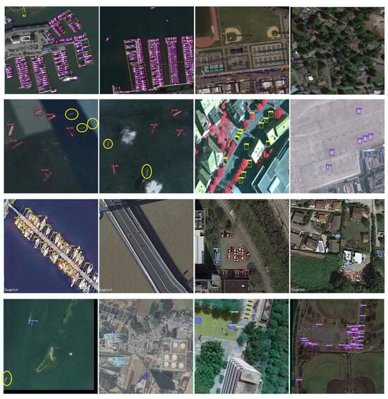
Figure 7.
Visualization of detection performance across four challenging aerial object detection datasets. Each row showcases examples from a different dataset. From top to bottom: DOTA, VHR-10, SIMD, and AI-TOD. Yellow ellipses indicate missed detections.
To better illustrate the advantages of the DCBANet over other methods, Figure 8 compares the detection results of the DCBANet and other advanced methods in challenging detection scenes. As shown, the proposed DCBANet generally achieves superior detection results compared to the other methods presented. Specifically, in the complex environment of Figure 8a, the DCBANet is the only method that can identify all small objects. Furthermore, for scenes with dense targets (Figure 8b) and shadow occlusion (Figure 8c), the DCBANet exhibits fewer missed detections and classification errors than the other advanced methods.
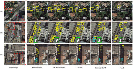
Figure 8.
Comparison of the performance of the DCBANet and other advanced methods in detecting small targets in challenging scenarios. (a) Complex environment. (b) Dense distribution. (c) Shadow occlusion. The first column represents the input image, and the second column represents the ground truth within red dashed bounding boxes. The last four columns are the detection results of DCBANet, LSKNet [14], Cascade-RCNN [24], and FCOS [62], respectively. The DCBANet achieves the best results.
5. Conclusions
In order to address the key challenges of small target detection in remote sensing images, we introduced DCBANet, a novel backbone network designed to dynamically perceive and adapt to contextual cues. Our contributions are threefold: (1) the DCSA Block, featuring a multi-branch architecture and internal CASM units, which adaptively capture contextual information across various receptive fields; (2) the EBA module, which intelligently fuses features from different branches by prioritizing the most informative ones; and (3) the lightweight DGFFN, which significantly reduces computational complexity while maintaining high performance.
Our comprehensive experiments on four challenging public datasets validate the superiority of our approach. The DCBANet achieves state-of-the-art mAP@0.5 scores of 80.79% on DOTA, 89.17% on NWPU VHR-10, and 80.27% on SIMD. More importantly, on the dedicated small object benchmark AI-TOD, our model achieves a remarkable 42.4% mAP@0.5:0.95, with significant improvements in small object-specific metrics () over previous methods. This robustly demonstrates that our dynamic context-aware design is highly effective for tackling the small object detection problem.
Despite these promising results, there remains room for improvement. Our current model focuses primarily on local context and could be enhanced by better integrating global scene-level information to improve performance on multi-scale and weakly defined targets. Future work will explore more advanced feature fusion techniques and aim to develop a more holistic context-aware system for Remote Sensing Object Detection.
Author Contributions
Conceptualization, H.J.; methodology, Y.S. and T.B.; software, H.J. and Y.S.; validation, H.J. and T.B.; writing—original draft preparation, Y.S. and T.B.; writing—review and editing, H.J. and T.B.; visualization, Y.C.; supervision, K.S. and T.B. All authors have read and agreed to the published version of the manuscript.
Funding
This work was supported by the Hubei Provincial Natural Science Foundation (Grant No. 2025AFB061), the Hubei University of Technology Doctoral Research Startup Project (Grant No. XJ2024004101), and the National Natural Science Foundation of China (Grant No. 42301457).
Data Availability Statement
The datasets presented in this study can be downloaded here: https://captain-whu.github.io/DOTA/dataset.html (DOTA). https://gcheng-nwpu.github.io/\#Datasets (NWPU VHR-10). https://github.com/ihians/simd (SIMD). https://github.com/jwwangchn/AI-TOD (AI-TOD).
Conflicts of Interest
The authors declare no conflicts of interest.
Abbreviations
The following abbreviations are used in this manuscript:
| RSOD | Remote Sensing Object Detection |
| RSIs | Remote Sensing Images |
| DCBANet | Dynamic Context Branch Attention Network |
| DCSA Block | Dynamic Context Scale-Aware Block |
| EBA | Efficient Branch Attention |
| FFN | Feedforward Network |
| DGFFN | Dual-Gated Feedforward Network |
| SGU | Spatial Gating Unit |
| CGU | Channel Gating Unit |
| MLP | Multilayer Perceptron |
| FLOPs | Floating-point Operations |
| AP | Average Precision |
| mAP | Mean Average Precision |
| FPS | Frames Per Second |
References
- Gui, S.; Song, S.; Qin, R.; Tang, Y. Remote Sensing Object Detection in the Deep Learning Era—A Review. Remote Sens. 2024, 16, 327. [Google Scholar] [CrossRef]
- Guo, Z.; Liu, C.; Zhang, X.; Jiao, J.; Ji, X.; Ye, Q. Beyond Bounding-Box: Convex-hull Feature Adaptation for Oriented and Densely Packed Object Detection. In Proceedings of the 2021 IEEE/CVF Conference on Computer Vision and Pattern Recognition (CVPR), Nashville, TN, USA, 20–25 June 2021; pp. 8788–8797. [Google Scholar] [CrossRef]
- Lyu, C.; Zhang, W.; Huang, H.; Zhou, Y.; Wang, Y.; Liu, Y.; Zhang, S.; Chen, K. RTMDet: An Empirical Study of Designing Real-Time Object Detectors. arXiv 2022, arXiv:2212.07784. [Google Scholar]
- Ding, J.; Xue, N.; Long, Y.; Xia, G.-S.; Lu, Q. Learning RoI Transformer for Oriented Object Detection in Aerial Images. In Proceedings of the 2019 IEEE/CVF Conference on Computer Vision and Pattern Recognition (CVPR), Long Beach, CA, USA, 15–20 June 2019; pp. 2844–2853. [Google Scholar] [CrossRef]
- Xie, X.; Cheng, G.; Wang, J.; Yao, X.; Han, J. Oriented R-CNN for Object Detection. In Proceedings of the 2021 IEEE/CVF International Conference on Computer Vision (ICCV), Montreal, QC, Canada, 10–17 October 2021; pp. 3500–3509. [Google Scholar] [CrossRef]
- Cheng, G.; Yuan, X.; Han, X.J. Towards Large Scale Small Object Detection: Survey and Benchmarks. IEEE Trans. Pattern Anal. Mach. Intell. 2023, 45, 13467–13488. [Google Scholar] [CrossRef]
- Chen, G.; Wang, H.; Chen, K.; Li, Z.; Song, Z. A Survey of the Four Pillars for Small Object Detection: Multiscale Representation, Contextual Information, Super-Resolution, and Region Proposal. IEEE Trans. Syst. Man Cybern. Syst. 2022, 52, 936–953. [Google Scholar] [CrossRef]
- Hua, X.; Cui, X.; Xu, X. Weakly Supervised Underwater Object Real-time Detection Based on High-resolution Attention Class Activation Mapping and Category Hierarchy. Pattern Recognit. 2025, 159, 111111. [Google Scholar] [CrossRef]
- Gao, T.; Xia, S.; Liu, M. MSNet: Multi-Scale Network for Object Detection in Remote Sensing Images. Pattern Recognit. 2025, 158, 110983. [Google Scholar] [CrossRef]
- Chen, C.; Zeng, W.; Zhang, X. HFPNet: Super Feature Aggregation Pyramid Network for Maritime Remote Sensing Small-Object Detection. IEEE J. Sel. Top. Appl. Earth Obs. Remote Sens. 2023, 16, 5973–5989. [Google Scholar] [CrossRef]
- Wei, C.; Bai, L.; Chen, X.; Han, J. Cross-Modality Data Augmentation for Aerial Object Detection with Representation Learning. Remote Sens. 2024, 16, 4649. [Google Scholar] [CrossRef]
- Cheng, G.; Wang, J.; Li, K.; Xie, X. Anchor-Free Oriented Proposal Generator for Object Detection. IEEE Trans. Geosci. Remote Sens. 2022, 60, 5625411. [Google Scholar] [CrossRef]
- Song, G.; Du, H.; Zhang, X. Small Object Detection in Unmanned Aerial Vehicle Images Using Multi-Scale Hybrid Attention. Eng. Appl. Artif. Intell. 2024, 128, 107455. [Google Scholar] [CrossRef]
- Li, Y.; Hou, Q.; Zheng, Z.; Cheng, M.-M.; Yang, J.; Li, X. Large Selective Kernel Network for Remote Sensing Object Detection. In Proceedings of the 2023 IEEE/CVF International Conference on Computer Vision (ICCV), Paris, France, 1–6 October 2023; pp. 16748–16759. [Google Scholar] [CrossRef]
- Cui, L.; Lv, P.; Jiang, X.; Gao, Z. Context-Aware Block Net for Small Object Detection. IEEE Trans. Cybern. 2022, 52, 2300–2313. [Google Scholar] [CrossRef]
- He, X.; Zheng, X.; Hao, X.; Jin, H.; Zhou, X.; Shao, L. Improving Small Object Detection via Context-Aware and Feature-Enhanced Plug-and-Play Modules. J. Real-Time Image Process. 2024, 21, 44. [Google Scholar] [CrossRef]
- Wu, C.; Zeng, Z. YOLOX-CA: A Remote Sensing Object Detection Model Based on Contextual Feature Enhancement and Attention Mechanism. IEEE Access 2024, 12, 84632. [Google Scholar] [CrossRef]
- Li, Z.; Wang, Y.; Zhang, Y. Context Feature Integration and Balanced Sampling Strategy for Small Weak Object Detection in Remote Sensing Imagery. IEEE Geosci. Remote Sens. Lett. 2024, 21, 6009105. [Google Scholar] [CrossRef]
- Ding, S.; Xiong, M.; Wang, X. Dynamic feature and context enhancement network for faster detection of small objects. Expert Syst. Appl. 2025, 265, 125732. [Google Scholar] [CrossRef]
- Yang, H.; Qiu, S. A Novel Dynamic Contextual Feature Fusion Model for Small Object Detection in Satellite Remote-Sensing Images. Information 2024, 15, 230. [Google Scholar] [CrossRef]
- Wang, B.; Ji, R.; Zhang, L. Learning to zoom: Exploiting mixed-scale contextual information for object detection. Expert Syst. Appl. 2025, 264, 125871. [Google Scholar] [CrossRef]
- Yang, X.; Liu, Q.; Yan, J.; Li, A. R3Det: Refined Single-Stage Detector with Feature Refinement for Rotating Object. arXiv 2019, arXiv:1908.05612. [Google Scholar] [CrossRef]
- Han, J.; Ding, J.; Li, J.; Xia, G. Align Deep Features for Oriented Object Detection. IEEE Trans. Geosci. Remote Sens. 2022, 60, 5602511. [Google Scholar] [CrossRef]
- Cai, Z.; Vasconcelos, N. Cascade R-CNN: Delving Into High Quality Object Detection. In Proceedings of the 2018 IEEE/CVF Conference on Computer Vision and Pattern Recognition (CVPR), Salt Lake City, UT, USA, 18–23 June 2018; pp. 6154–6162. [Google Scholar] [CrossRef]
- Zhang, H.; Chang, H.; Ma, B. Dynamic R-CNN: Towards High Quality Object Detection via Dynamic Training. In Computer Vision–ECCV 2020; Lecture Notes in Computer Science, Volume 12360; Vedaldi, A., Bischof, H., Brox, T., Frahm, J.-M., Eds.; Springer: Cham, Switzerland, 2020; pp. 260–275. [Google Scholar] [CrossRef]
- Ren, S.; He, K.; Girshick, R.; Sun, J. Faster R-CNN: Towards Real-Time Object Detection with Region Proposal Networks. IEEE Trans. Pattern Anal. Mach. Intell. 2017, 39, 1137–1149. [Google Scholar] [CrossRef]
- Carion, N.; Massa, F.; Synnaeve, G.; Usunier, N.; Kirillov, A.; Zagoruyko, S. End-to-End Object Detection with Transformers. In Computer Vision–ECCV 2020; Lecture Notes in Computer Science, Volume 12346; Vedaldi, A., Bischof, H., Brox, T., Frahm, J.-M., Eds.; Springer: Cham, Switzerland, 2020; pp. 213–229. [Google Scholar] [CrossRef]
- Zhao, J.; Ding, Z.; Zhou, Y.; Zhu, H.; Du, W. OrientedFormer: An End-to-End Transformer-Based Oriented Object Detector in Remote Sensing Images. IEEE Trans. Geosci. Remote Sens. 2024, 62, 5640816. [Google Scholar] [CrossRef]
- Zhu, X.; Su, W.; Lu, L. Deformable DETR: Deformable Transformers for End-to-End Object Detection. In Proceedings of the International Conference on Learning Representations (ICLR), Vienna, Austria, 3–7 May 2021; pp. 1–16. [Google Scholar]
- Yang, C.; Huang, Z.; Wang, N. QueryDet: Cascaded Sparse Query for Accelerating High-Resolution Small Object Detection. In Proceedings of the 2022 IEEE/CVF Conference on Computer Vision and Pattern Recognition (CVPR), New Orleans, LA, USA, 18–24 June 2022; pp. 13658–13667. [Google Scholar] [CrossRef]
- Deng, C.; Wang, M.; Liu, L. Extended Feature Pyramid Network for Small Object Detection. IEEE Trans. Multimed. 2022, 24, 1968–1979. [Google Scholar] [CrossRef]
- Zeng, N.; Wu, P.; Wang, Z. A Small-Sized Object Detection Oriented Multi-Scale Feature Fusion Approach with Application to Defect Detection. IEEE Trans. Instrum. Meas. 2022, 71, 3507014. [Google Scholar] [CrossRef]
- Liu, Y.; Li, Q.; Yuan, Y.; Du, Q.; Wang, Q. ABNet: Adaptive Balanced Network for Multiscale Object Detection in Remote Sensing Imagery. IEEE Trans. Geosci. Remote Sens. 2022, 60, 5614914. [Google Scholar] [CrossRef]
- Yang, X.; Yan, J.; Liao, W.; Yang, X.; Tang, J.; He, T. SCRDet++: Detecting Small, Cluttered and Rotated Objects via Instance-Level Feature Denoising and Rotation Loss Smoothing. IEEE Trans. Pattern Anal. Mach. Intell. 2023, 45, 2384–2399. [Google Scholar] [CrossRef]
- Vaswani, A.; Shazeer, N.M.; Parmar, N. Attention is All You Need. In Proceedings of the 31st Conference on Neural Information Processing Systems (NeurIPS), Long Beach, CA, USA, 4–9 December 2017. [Google Scholar]
- Guo, M.; Xu, T.; Liu, J. Attention Mechanisms in Computer Vision: A Survey. Comput. Vis. Media 2022, 8, 331–368. [Google Scholar] [CrossRef]
- Hu, J.; Shen, L.; Sun, G. Squeeze-and-Excitation Networks. In Proceedings of the 2018 IEEE/CVF Conference on Computer Vision and Pattern Recognition (CVPR), Salt Lake City, UT, USA, 18–23 June 2018; pp. 7132–7141. [Google Scholar] [CrossRef]
- Wang, Q.; Wu, B.; Zhu, P. ECA-Net: Efficient Channel Attention for Deep Convolutional Neural Networks. In Proceedings of the 2020 IEEE/CVF Conference on Computer Vision and Pattern Recognition (CVPR), Seattle, WA, USA, 13–19 June 2020; pp. 11531–11539. [Google Scholar] [CrossRef]
- Hu, J.; Shen, L.; Albanie, S.; Sun, G.; Vedaldi, A. Gather-Excite: Exploiting Feature Context in Convolutional Neural Networks. arXiv 2018, arXiv:1810.12348. [Google Scholar] [CrossRef]
- Zhao, H.; Zhang, Y.; Liu, S.; Shi, J. PSANet: Point-wise Spatial Attention Network for Scene Parsing. In Computer Vision–ECCV 2018; Lecture Notes in Computer Science, Vol. 11213; Ferrari, V., Hebert, M., Sminchisescu, C., Weiss, Y., Eds.; Springer: Cham, Switzerland, 2018; pp. 270–286. [Google Scholar] [CrossRef]
- Dosovitskiy, A.; Beyer, L.; Kolesnikov, A. An Image is Worth 16 × 16 Words: Transformers for Image Recognition at Scale. arXiv 2020, arXiv:2010.11929. [Google Scholar]
- Zhang, H.; Wu, C.; Zhang, Z.; Zhu, Y. ResNeSt: Split-Attention Networks. In Proceedings of the 2022 IEEE/CVF Conference on Computer Vision and Pattern Recognition Workshops (CVPRW), New Orleans, LA, USA, 19–20 June 2022; pp. 2735–2745. [Google Scholar] [CrossRef]
- Liu, Z.; Lin, Y.; Cao, Y.; Hu, H.; Wei, Y.; Zhang, Z.; Lin, S.; Guo, B. Swin Transformer: Hierarchical Vision Transformer Using Shifted Windows. In Proceedings of the 2021 IEEE/CVF International Conference on Computer Vision (ICCV), Montreal, QC, Canada, 10–17 October 2021; pp. 9992–10002. [Google Scholar] [CrossRef]
- Chen, Z.; Zhu, Y.; Li, Z.; Yang, F.; Zhao, C.; Wang, J.; Tang, M. The Devil is in Details: Delving Into Lite FFN Design for Vision Transformers. In Proceedings of the ICASSP 2024–2024 IEEE International Conference on Acoustics, Speech and Signal Processing (ICASSP), Seoul, Republic of Korea, 14–19 April 2024; pp. 4130–4134. [Google Scholar] [CrossRef]
- Xu, H.; Zhou, Z.; He, D. Vision Transformer with Attention Map Hallucination and FFN Compaction. arXiv 2023, arXiv:2306.10875. [Google Scholar]
- Yang, Z.; Zhu, L.; Wu, Y. Gated Channel Transformation for Visual Recognition. In Proceedings of the 2020 IEEE/CVF Conference on Computer Vision and Pattern Recognition (CVPR), Seattle, WA, USA, 13–19 June 2020; pp. 11791–11800. [Google Scholar] [CrossRef]
- Wang, Y.; Li, Y.; Wang, G. Multi-Scale Attention Network for Single Image Super-Resolution. In Proceedings of the 2024 IEEE/CVF Conference on Computer Vision and Pattern Recognition Workshops (CVPRW), Seattle, WA, USA, 17–18 June 2024; pp. 5950–5960. [Google Scholar] [CrossRef]
- Li, S.; Wang, Z.; Liu, Z.; Tan, C.; Lin, H.; Wu, D.; Chen, Z.; Zheng, J.; Li, S. MogaNet: Multi-Order Gated Aggregation Network. In Proceedings of the International Conference on Learning Representations (ICLR), Toulon, France, 25–29 April 2022. [Google Scholar]
- Guo, M.H.; Lu, C.Z.; Liu, Z.N.; Cheng, M.M.; Hu, S.M. Visual Attention Network. Comput. Vis. Media 2023, 9, 733–752. [Google Scholar] [CrossRef]
- Yu, W.; Si, C.; Zhou, P.; Luo, M. MetaFormer Baselines for Vision. IEEE Trans. Pattern Anal. Mach. Intell. 2024, 46, 896–912. [Google Scholar] [CrossRef]
- Xia, G.-S.; Bai, X.; Ding, J.; Zhu, Z. DOTA: A Large-Scale Dataset for Object Detection in Aerial Images. In Proceedings of the 2018 IEEE/CVF Conference on Computer Vision and Pattern Recognition (CVPR), Salt Lake City, UT, USA, 18–23 June 2018; pp. 3974–3983. [Google Scholar] [CrossRef]
- Haroon, M.; Shahzad, M.; Fraz, M. Multisized Object Detection Using Spaceborne Optical Imagery. IEEE J. Sel. Top. Appl. Earth Obs. Remote Sens. 2020, 13, 3032–3046. [Google Scholar] [CrossRef]
- Cheng, G.; Han, J.; Zhou, P. Multi-Class Geospatial Object Detection and Geographic Image Classification Based on Collection of Part Detectors. ISPRS J. Photogramm. Remote Sens. 2014, 98, 119–132. [Google Scholar] [CrossRef]
- Wang, J.; Yang, W.; Guo, H.; Zhang, R.; Xia, G. Tiny Object Detection in Aerial Images. In Proceedings of the 2020 25th International Conference on Pattern Recognition (ICPR), Milan, Italy, 10–15 January 2021; pp. 3791–3798. [Google Scholar] [CrossRef]
- Zeng, Y.; Chen, Y.; Yang, X. ARS-DETR: Aspect Ratio-Sensitive Detection Transformer for Aerial Oriented Object Detection. IEEE Trans. Geosci. Remote Sens. 2024, 62, 5610315. [Google Scholar] [CrossRef]
- Xie, X.; Cheng, G.; Rao, C. Oriented Object Detection via Contextual Dependence Mining and Penalty-Incentive Allocation. IEEE Trans. Geosci. Remote Sens. 2024, 62, 5618010. [Google Scholar] [CrossRef]
- Hou, L.; Lu, K.; Xue, J. Shape-Adaptive Selection and Measurement for Oriented Object Detection. In Proceedings of the AAAI Conference on Artificial Intelligence; 2022; Volume 36, pp. 923–932. [Google Scholar] [CrossRef]
- Cheng, G.; Yao, Y.; Li, S.; Li, K. Dual-Aligned Oriented Detector. IEEE Trans. Geosci. Remote Sens. 2022, 60, 5618111. [Google Scholar] [CrossRef]
- Han, J.; Ding, J.; Xue, N.; Xia, G. ReDet: A Rotation-Equivariant Detector for Aerial Object Detection. In Proceedings of the 2021 IEEE/CVF Conference on Computer Vision and Pattern Recognition (CVPR), Nashville, TN, USA, 20–25 June 2021; pp. 2785–2794. [Google Scholar] [CrossRef]
- Lin, T.; Goyal, P.; Girshick, R. Focal Loss for Dense Object Detection. IEEE Trans. Pattern Anal. Mach. Intell. 2020, 42, 318–327. [Google Scholar] [CrossRef]
- Tian, Z.; Shen, C.; Chen, H. FCOS: Fully Convolutional One-Stage Object Detection. In Proceedings of the 2019 IEEE/CVF International Conference on Computer Vision (ICCV), Seoul, Republic of Korea, 27 October–2 November 2019; pp. 9626–9635. [Google Scholar] [CrossRef]
- Chen, Q.; Wang, Y.; Yang, T. You Only Look One-Level Feature. In Proceedings of the 2021 IEEE/CVF Conference on Computer Vision and Pattern Recognition (CVPR), Nashville, TN, USA, 19–25 June 2021; pp. 13034–13043. [Google Scholar] [CrossRef]
- Xie, S.; Girshick, R.; Dollár, P.; Tu, Z.; He, K. Aggregated Residual Transformations for Deep Neural Networks. In Proceedings of the 2017 IEEE Conference on Computer Vision and Pattern Recognition (CVPR), Honolulu, HI, USA, 21–26 July 2017; pp. 5987–5995. [Google Scholar] [CrossRef]
Disclaimer/Publisher’s Note: The statements, opinions and data contained in all publications are solely those of the individual author(s) and contributor(s) and not of MDPI and/or the editor(s). MDPI and/or the editor(s) disclaim responsibility for any injury to people or property resulting from any ideas, methods, instructions or products referred to in the content. |
© 2025 by the authors. Licensee MDPI, Basel, Switzerland. This article is an open access article distributed under the terms and conditions of the Creative Commons Attribution (CC BY) license (https://creativecommons.org/licenses/by/4.0/).