Abstract
Visual geolocalization for aerial vehicles based on an analysis of Earth observation imagery is an effective method in GNSS-denied environments. However, existing methods for geographic location estimation have limitations: one relies on high-precision geodetic elevation data, which is costly, and the other assumes a flat ground surface, ignoring elevation differences. This paper presents a novel aerial vehicle geolocalization method. It integrates 2D information and relative depth information, which are both from Earth observation images. Firstly, the aerial and reference remote sensing satellite images are fed into a feature-matching network to extract pixel-level feature-matching pairs. Then, a depth estimation network is used to estimate the relative depth of the satellite remote sensing image, thereby obtaining the relative depth information of the ground area within the field of view of the aerial image. Finally, high-confidence matching pairs with similar depth and uniform distribution are selected to estimate the geographic location of the aerial vehicle. Experimental results demonstrate that the proposed method outperforms existing ones in terms of geolocalization accuracy and stability. It eliminates reliance on elevation data or planar assumptions, thus providing a more adaptable and robust solution for aerial vehicle geolocalization in GNSS-denied environments.
1. Introduction
In recent years, aerial vehicles have been widely used in agriculture, logistics, military operations, disaster rescue, and environmental monitoring [1,2,3,4,5]. The Global Navigation Satellite System (GNSS) serves as the primary approach for aerial vehicle geolocalization. However, aerial vehicles struggle to achieve autonomous geolocalization in GNSS-denied environments. Advances in computer vision have established vision-based perception as the preferred solution for this challenge. This approach follows a progressive three-tiered architecture: cross-domain image retrieval, heterogeneous image matching, and geographic location estimation. Related works in this domain are outlined below.
Cross-domain image retrieval can be defined as the process of utilizing aerial images to identify the most similar ones in a database of satellite remote sensing images, thereby establishing indexing relationships. Traditional methods have relied on hand-crafted features to capture the semantic content of images [6,7]. Compared to traditional systems, recent advancements in deep neural networks have significantly enhanced the performance of content-based retrieval. Unar et al. [8] utilized VGG16 and ResNet50 for feature extraction, improving the semantic information of the feature learner by employing multi-kernel feature learning to identify the most critical image-representation features. Meanwhile, Yamani et al. [9] combined Transformer encoders with CNN-based feature extractors to derive advanced semantic interpretations. Meng et al. [10] utilize DINOV2 [11] to extract features from aerial, satellite, and image sources, and VLAD [12] vectors are employed to combine sequential images with particle filters for the purpose of image retrieval.
Heterogeneous image matching establishes pixel-level feature correspondences between aerial and satellite remote sensing imagery. Traditional approaches relied on hand-crafted feature detection algorithms, such as Scale-Invariant Feature Transform (SIFT) [13], Speeded-Up Robust Features (SURF) [14], and Oriented FAST and Rotated BRIEF (ORB) [15]. Saleem et al. [16] proposed an improved SIFT algorithm based on normalized gradient enhancement. The RIFT algorithm, introduced by Li et al. [17], significantly enhanced feature point robustness and achieved rotation invariance. However, traditional algorithms exhibit limitations due to sensor discrepancies, inconsistent resolutions, and viewpoint variations inherent in cross-source imagery. In recent years, deep learning has revolutionized traditional feature extraction and matching techniques, gradually evolving from sparse feature extraction and matching to end-to-end dense matching. Han et al. [18] utilizes a convolutional neural network (CNN) to extract features from image patches. DeTone et al. [19] pioneered self-supervised joint feature detection and description with SuperPoint. Subsequently, Sarlin et al. [20] introduced SuperGlue, which incorporates a graph attention network (GAT) to model feature matching as a structural optimization problem between two views. SuperPoint combined with SuperGlue has become a paradigm for feature point extraction and matching. Lindenberger et al. [21] designed an adaptive pruning mechanism for LightGlue to address real-time bottlenecks, improving inference speed by 2-3 times while maintaining accuracy. Furthermore, Sun et al. [22] proposed LoFTR, which completely overturned the “detect-match” divide-and-conquer paradigm.
Geographic location estimation refers to calculating the position of the aerial vehicle using image-matching results to obtain longitude and latitude coordinates. Wang et al. [23] computed homography transformations based on the matching results of aerial and satellite imagery, subsequently employing the projection coordinates of the aerial image’s center pixel onto the satellite image as the aerial vehicle geolocalization. This methodology yields accurate positioning results exclusively when the onboard camera is oriented in a nadir-view configuration. Yao et al. [24] leveraged ground elevation data, in conjunction with feature matching results, to formulate a 3D-2D Perspective-n-Point (PnP) problem, employing algorithms such as EPnP [25] to determine the aerial vehicle’s geographic location. Following the establishment of a matching relationship between aerial image pixel coordinates and real-world geographic coordinates [26,27,28], a planar scene constraint is assumed, wherein all geographic points lie on a horizontal plane, thereby enabling the formulation and solution of a PnP problem. Li et al. [29] derived a homography transformation between aerial image pixel coordinates and road network geographic coordinates, predicated on the assumption of a horizontal plane. By computing the homography matrix H and subsequently decomposing it, the geographic location of the aerial vehicle can be determined.
Contemporary research predominantly focuses on cross-domain image retrieval and heterogeneous image matching, with relatively limited attention devoted to geographic location estimation. Current estimation methods primarily depend on either a priori geographic elevation data or planar terrain assumptions. The former approach is constrained by insufficient data accuracy and regional data gaps, while the latter introduces errors by disregarding actual topographic undulations and elevation variations. To address these limitations, this paper presents an innovative visual geolocalization method for aerial vehicles that integrates satellite remote sensing imagery with relative depth information. This approach significantly enhances geolocalization accuracy and stability in complex terrain environments. The principal contributions of this work are detailed below:
- We have conducted an error analysis of the planar assumption-based method for aerial vehicle geolocalization.
- We propose a novel method for aerial vehicle geolocalization that leverages relative depth consistency from satellite remote sensing imagery.
2. Materials and Methods
2.1. Problem Definition
Map projection transforms geodetic coordinates into planimetric map coordinates. The Pseudo-Mercator Projection (EPSG:3857), widely adopted by web mapping services like Google Maps, establishes its coordinate origin at the equator–prime meridian intersection. This system extends eastward along the positive X-axis and northward along the positive Y-axis. The X-axis and Y-axis take values in the range [−20,037,508.3427892, 20,037,508.3427892] in m units. Under the Pseudo-Mercator Projection, the geodetic coordinates of a terrestrial point are defined as , with longitude constrained to and latitude bound with . The corresponding Mercator plane coordinates are derived through
where represents the radius of the Earth, which is 6378137 m, and and are the radians of the and . This study establishes a global coordinate system with the following definitions:
- X/Y-axis Definition: The X-Y plane originates at the intersection of the Earth’s equator (0° latitude) and prime meridian (0° longitude), with axis orientations aligned with the Pseudo-Mercator coordinate system-X-axis positive eastward and Y-axis positive northward.
- Z-axis Definition: A local vertical axis originates from the aerial vehicle’s takeoff position, orthogonal to the X-Y plane, with a positive direction aligned with the upward vector in the East–North–Up (ENU) geodetic frame.
This study addresses the following problem: In the world coordinate system, given a satellite remote sensing reference image and the Mercator coordinates of each of its pixels, the aim is to geolocate the aerial vehicle based on aerial images.
2.2. Error Analysis in Aerial Vehicle Geolocalization Under Planar Assumption
Image-matching geolocalization establishes pixel-to-geographic coordinate mappings using satellite imagery. When elevation data are unavailable, geographic positions are calculated under a planar terrain assumption. However, actual terrain variations and building heights introduce localization errors. This section analyzes errors attributable to the planar assumption.
Let denote the world coordinates of a geographical point, and represent its corresponding pixel coordinates in an aerial image. The elevation within the image coverage area follows a Gaussian distribution . Under the plane hypothesis, spatial points are approximated as . Define the true pose of the aerial vehicle as and , and the estimated pose as and . The PnP problem is established based on the projection relationship between pixel points and geographical points for pose solution.
Actual Reprojection Error:
Assuming a planar configuration, the reprojection error can be defined as follows:
Among them, is the internal parameter matrix of the camera; is the depth value of in the camera coordinate system under the true pose; and is the depth value of in the estimated pose under the planar assumption. When the re-projection errors E and converge to zero through optimization, the normalized camera coordinate direction vectors projected to the same point by the real model and the planar hypothetical model must be equal. The difference between the depth scale and is compensated by the pose error, and we can approximately obtain
where , and , respectively. Assume that and . and are the pose errors caused by the planar assumption, where and . By substituting and into Equation (4), one obtains
By conducting a first-order Taylor expansion on the term associated with rotational disturbances, we can obtain
Assume that ; then, we can obtain
The mathematical expectation of is as follows:
Assume that and . We can then obtain
It can be inferred that the expected value of the translation vector error comprises two components: the first component is the compensation error attributable to elevation data, while the second component arises from coupling errors associated with rotational disturbances and the arrangement of two-dimensional geographic coordinates. The equation suggests that an increase in the mean elevation of geographic points correlates with a corresponding increase in the translation vector error as determined by the PnP method under the assumption of a planar configuration.
2.3. Geographic Location Estimate Method for the Aerial Vehicle with Consistent Relative Depth
The coordinates of a geographical point in the world coordinate system are . Here, X and Y are known Mercator coordinates, while the height information for Z is unknown. Satellite remote sensing images use orthographic projection, where each pixel in the image corresponds one-to-one with a geographic point. By performing depth estimation on the satellite images, we obtain relative depth information for each pixel, with output values ranging from 0 to 255. The relative depth value is inversely proportional to the distance from the geographic point to the shooting point; a smaller value indicates a greater distance, while a larger value indicates a closer distance. Additionally, the depth value is positively correlated with the relative height of the geographic point; a larger value corresponds to a higher elevation, while a smaller value corresponds to a lower elevation.
Within the ideal geometric model of satellite orthoimages, assuming the camera height is H, the absolute depth of a geographical point in the same image can be calculated using the formula:
where D represents the absolute depth, d represents the relative depth, and c represents the scale factor which has a unit of m. Assuming the elevation value of the camera is H, and the elevation value of a certain geographical point is , we can obtain
Therefore,
Thus, when the relative depth is the same, the actual terrain elevation data should also be consistent. Select the geographical coordinate , ensuring that it maintains the same relative depth d. Find the coordinate system such that in this coordinate system is and name this coordinate system the reference coordinate system. We can easily determine that , . and represent the rotation matrix and translation vector from the world coordinate system to the reference coordinate system, respectively, and the following can be obtained:
In the case of , assume that the homogeneous coordinate of pixel corresponding to the aerial image is . Then, the coordinates and in the reference coordinate system satisfy the projection relationship as follows:
where s is the scale factor, and are the rotation matrix and translation vector from the reference coordinate system to the aerial vehicle coordinate system, respectively. Let , where represents the column i vector. We can then obtain
Expanding Equation (15) yields
Let
We can then determine that and satisfy the homography transformation. is the homologous transformation matrix from to . Let and , where represents the matrix column i vector. Then, conduct Singular Value Decomposition (SVD) on matrices and :
where . According to the conclusion of [29], let and . Then, we can obtain
where and are the first two columns of .
The coordinates of the aircraft in the world coordinate system are
where
Substituting it into Equation (20) gives
Writing , we can obtain
represents the coordinates of the aerial vehicle in the world coordinate system. The theoretical analysis indicates that when selecting geographical points with identical relative depth, the position of the aerial vehicle in the pseudo-Mercator coordinate system, namely , can be accurately determined. Subsequently, by applying Equation (24), the conversion from to longitude and latitude coordinates can be achieved, thereby identifying the geographic location of the aerial vehicle.
2.4. Satellite Remote Sensing Image with Relative Depth-Assisted Aerial Vehicle Geolocalization Method
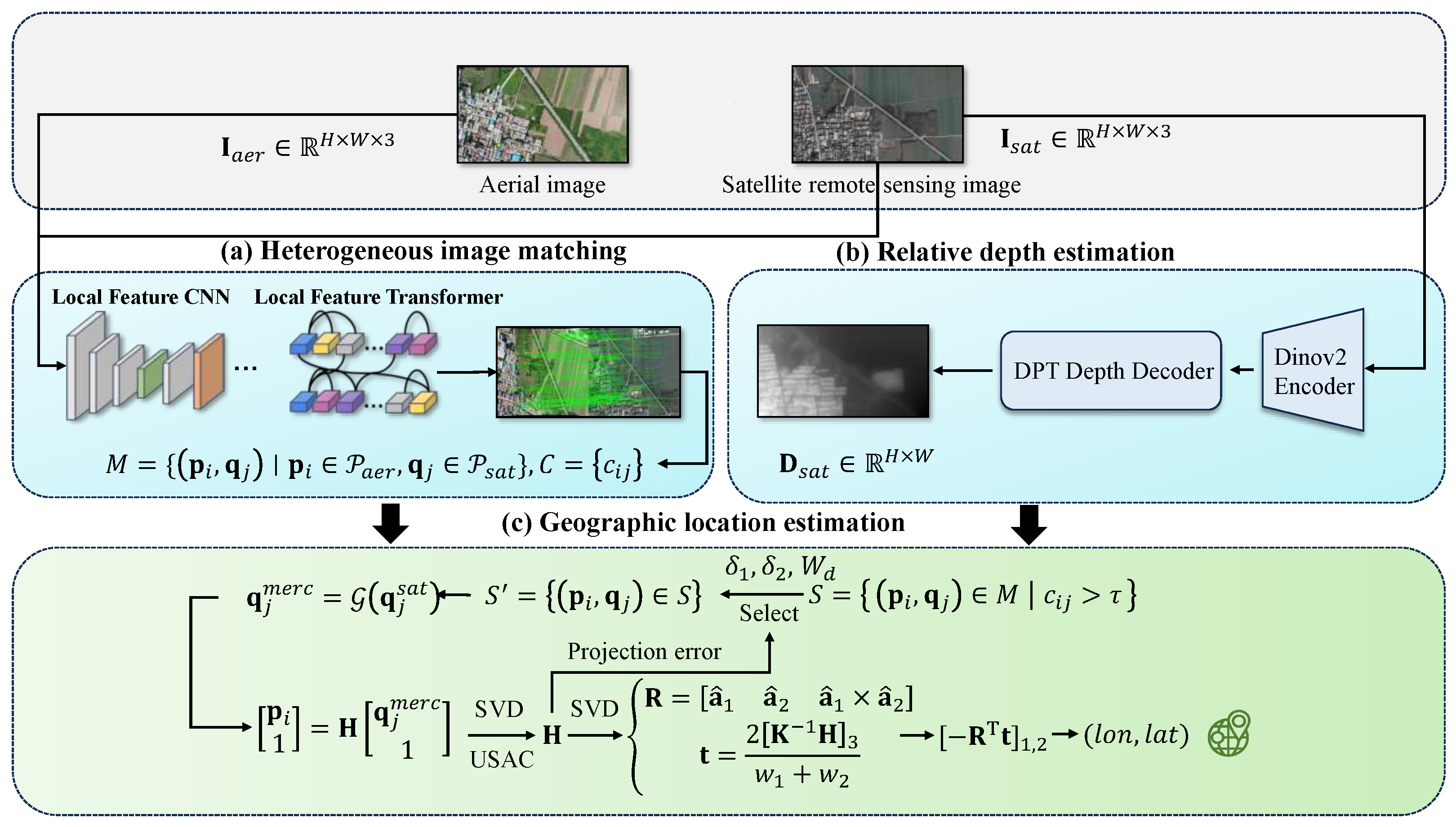
The methodology presented in this study consists of three core components: (a) a heterogeneous image-matching module, (b) a relative depth estimation module, and (c) a geographic location estimation module. As shown in Figure 1, the approach takes aerial images and their corresponding satellite remote sensing images as input. These aerial and satellite images are first processed by the heterogeneous image-matching module to extract matched feature pairs and their associated confidence levels. The satellite remote sensing image is then channeled into the relative depth estimation module to generate its corresponding relative depth map. Finally, the matched feature pairs, their confidence levels, and the satellite-derived relative depth map are input to the geographic location estimation module. This module integrates these inputs to accurately estimate the geographic location of the aerial vehicle.

Figure 1.
Overall framework of the proposed aerial vehicle geolocalization method. The steps in numerals (a–c) introduce the localization procedure. The captured aerial vehicle image and reference satellite remote sensing image from one of our experiments are shown. (a) Heterogeneous image matching. (b) Relative depth estimation. (c) Geographic location. In the figure, SVD presents “Singular Value Decomposition” and USAC presents “A Universal Framework for Random Sample Consensus” estimation.
2.4.1. Heterogeneous Image Matching
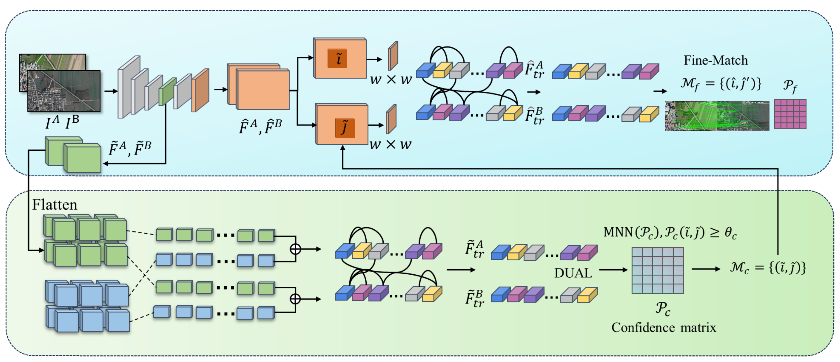
Heterogeneous image matching is facilitated by the use of LoFTR [22]. This method adeptly addresses cross-modal discrepancies through its end-to-end architecture, which operates without the need for detectors. It employs global modeling via Transformers and integrates fine-to-coarse granularity fusion. Notably, LoFTR is capable of producing dense and highly accurate matching point pairs even in scenes characterized by low texture and non-linear variations. The framework of this approach is illustrated in Figure 2.

Figure 2.
Heterogenous image-matching network.
The aerial image and the satellite remote sensing image are inputted into using the CNN feature extraction network to extract rough feature maps and of 1/8 size of the original image for quick screening of candidate matching regions. Fine feature maps and of 1/2 size retaining more details are used for precise localization.
Then, and are expanded, and positional encoding is added to the LoFTR module for processing to extract positional and context-dependent local features to obtain and . and are input into the differentiable matching layer to compute the score matrix between the features:
When the dual-softmax micromatchable layer is then used, the matching confidence matrix is obtained:
The matches are then selected based on confidence thresholds and mutual proximity criteria:
The coarse matching prediction is obtained. For each coarse matching result , the position is centered in the fine feature maps , . Then, the center vectors of are correlated with all the vectors of , respectively, to generate the heatmap, which represents the probability of matching each pixel in the neighborhood of with . Finally, the expectation value on the probability distribution is calculated to bring the coarse matching result up to the sub-pixel matching level to obtain the final matching result .
2.4.2. Relative Depth Estimation
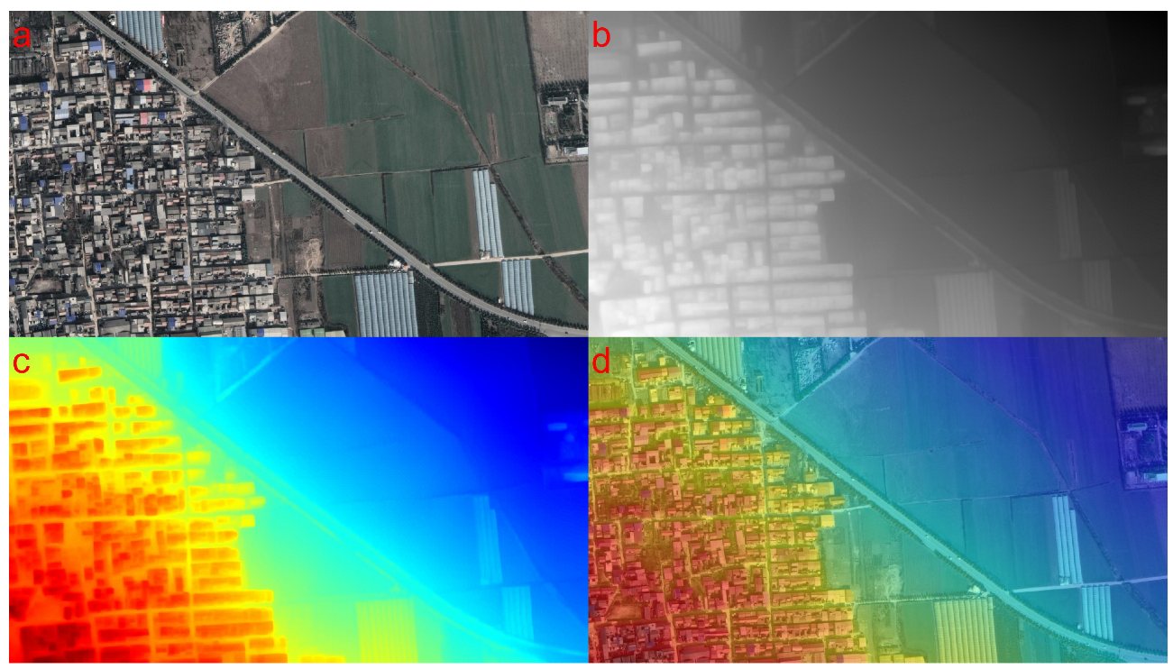
The relative depth estimation module uses the Depth Anything V2 model [30], which, in contrast to its predecessor V1 [31], uses fully synthetic images in place of all labeled real images and incorporates semantic information to train the teacher model. Reliable teacher models are trained based on high-quality synthetic images DINOv2-G. Pseudo-depth is generated using the teacher model on large-scale unlabeled real images. Student models, on the other hand, are trained based on pseudo-labeled real images for robust generalization. The training used five exact synthetic datasets (595,000 images) and eight large-scale pseudo-labeled real datasets (62 million images). Using the pseudo-labeling generated by the above exploits, ref. [30] trained four student models of different sizes (Small/Base/Large/Giant). Student models acquired the ability to make accurate depth predictions on real images by mimicking the teacher model’s behavior. The geometric constraints of nadir-view orthographic projection in satellite imagery position the imaging plane approximately perpendicular to the ground surface; consequently, relative depth differences between pixels directly correspond to changes in surface elevation. We therefore employ the Large variant to estimate satellite image depth, generating a 0–255 grayscale map representing relative depth. Lower values indicate smaller elevation values, while higher values signify greater elevation. Relative depth estimation is illustrated in Figure 3.

Figure 3.
Relative depth estimation. (a) The satellite remote sensing image; (b) the depth grayscale map output by the depth estimation model; (c) the result of converting the grayscale map into a heatmap; and (d) the overlay of the heatmap with the original satellite image. In the figure, the color representation rule is as follows: the redder the color, the greater the depth value, indicating a higher elevation; the bluer the color, the smaller the depth value, indicating a lower elevation.
2.4.3. Geographic Location Estimation
Denote the feature point matching set of the aerial image and the satellite remote sensing image as , where and denote the feature point sets of the aerial image and the satellite remote sensing image, respectively. The feature point coordinates and are pixel coordinates. Meanwhile, let be the matching confidence level of and . Let the relative depth estimation result of the satellite remote sensing image be denoted as , a grayscale image composed of 0-255.
First, screen through the confidence threshold and take 0.3. The filtered matching set is
The relative depth values of aerial image feature points are determined by , where . Feature points with the same depth value are selected using the depth consistency constraint. Since depth estimation has errors, the windowing mechanism is chosen. A dynamic depth window is constructed, where is the standard deviation of the depth values of the feature points of the aerial image. The sliding window mechanism is then used to traverse and select the subset .
Next, a triple constraint is imposed on the candidate subset. The first is the subset size constraint; to ensure that a single-response matrix computation can be performed, the number of matches in the subset needs to be larger than 4. The second is the confidence constraint; to ensure the matching quality of the subset, the average confidence of the matched pairs needs to be larger than the threshold value of . does not use a fixed value and represents the average confidence level of the matching pairs. The third is the spatial distribution constraint; to ensure that the distribution of the feature points in the subset is uniform, we use the convex hull area of the feature points of aerial images in the selected subset to carve out the area of convex bags. The greater the convex hull area is over the area of the image, the more uniform its distribution is. The larger the area is, the more uniform its distribution is. The projected coordinates of the candidate subset on the aerial image are , and its convex hull area is computed by Graham’s scanning algorithm:
The ratio of convex hull area to image area needs to be satisfied:
The parameter is adaptively determined through a dynamic selection strategy based on the depth window . An increased value signifies substantial relative depth variations within the region, thereby necessitating a higher threshold to enforce enhanced spatial homogeneity of feature correspondences. Conversely, a diminished indicates limited depth disparity, permitting relaxation of the threshold. This adaptive mechanism is formally expressed as
where , , and .
At this point, the candidate subset are points approximately in the same plane. The candidate subset satisfying the above three constraints is subjected to the computation of the homography matrix. Let the mapping relation from the pixel coordinates to the Mercator coordinates of the satellite map be
where is the known geographical alignment function and . The geographical alignment function is
where are the Mercator coordinates and are the Mercator coordinates corresponding to the pixels in the upper left corner of the satellite remote sensing image. The spatial resolution of the d satellite remote sensing image represents the actual distance corresponding to a single pixel.
For , establish the projection relationship from the pixel coordinates of the aerial image to the Mercator coordinates:
where is the homogeneous coordinate of the feature points in the aerial image and is the Mercator homogeneous coordinate. is the homography matrix. Expanding Equation (34), we can obtain
For that meets the conditions, solve the homography matrix and calculate the projection error of the inner points. Select the one with the most minor error, . Then, based on the derivation in Section 2.3, decompose to obtain and :
The geographic location of the aerial vehicle in the Mercator coordinate system is . The geographic location of the aerial vehicle can be obtained by bringing into Equation (24).
3. Results
3.1. Dataset
3.1.1. Aerial Data of the Aerial Vehicle
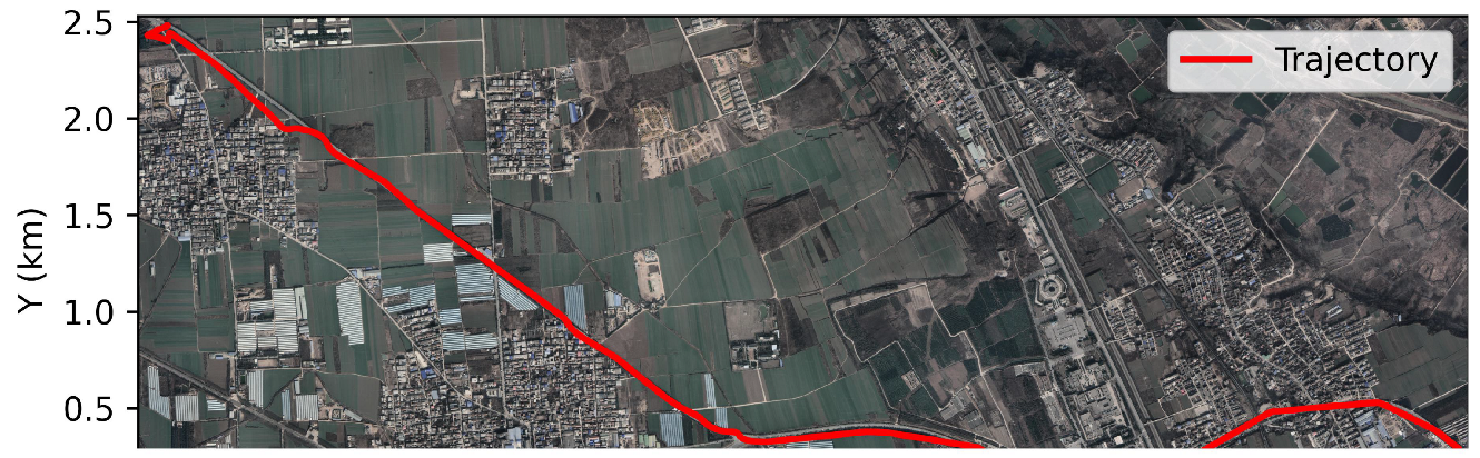
To address the scarcity of publicly available aerial image datasets, we deployed a DJI M300 UAV equipped with an H20 gimbal camera (featuring an integrated RTK localization system) to capture aerial imagery over suburban Xi’an, China. This platform acquired images with precise geographic coordinates and attitude parameters. The resulting aerial video spans 7.9968 km, with altitudes ranging from 13 to 603 m, for a duration of 968 s, and a frame rate of 30 FPS. We compiled these data into a validation-ready benchmark dataset covering complex geomorphological areas featuring significant elevation variations, including representative terrain features such as building clusters, transportation networks, and vegetated zones. All images feature 1920 × 1080 resolution. The complete flight track recorded during the experiment is shown in Figure 4.

Figure 4.
Trajectory of the aerial vehicle in flight.
3.1.2. Satellite Remote Sensing Imagery Data
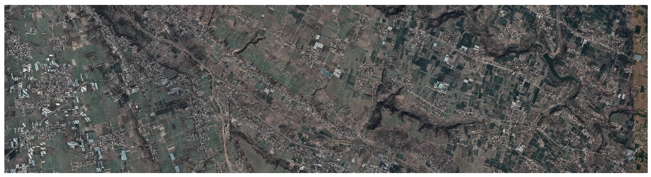
We used the Google Maps platform to acquire a high-resolution satellite remote sensing map covering the target area. As shown in Figure 5, the satellite image covers a rectangular area spanning about 31.2 km from east to west and extending about 5.8 km from north to south, with a geospatial extent of 181 km2. The image adopts 24-bit true color coding (RGB three-band), and the pixel matrix dimension is 26,905 × 7032, which meets the requirement of wide coverage.

Figure 5.
Satellite remote sensing map.
Table 1 shows the coordinate parameters of the four boundary points of the satellite remote sensing map containing two coordinate systems, the Web Mercator projected coordinate system (EPSG:3857) and the WGS84 geographic coordinate system (EPSG:4326). The spatial resolution of the map is 1 m/pixel.

Table 1.
Satellite remote sensing map boundary coordinates.
3.1.3. Aerial Image—Satellite Remote Sensing Image-Matching Dataset
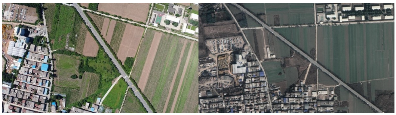
A matching pair of the aerial image and the satellite remote sensing map is ultimately created, as illustrated in Figure 6, after the corresponding area on the satellite remote sensing reference map is precisely matched based on the aerial image’s actual position. A satellite image of the same size as the aerial image is then cropped out.

Figure 6.
Aerial image—satellite remote sensing image-matching pair.
In order to create a matched dataset of aerial and satellite images, we chose frame sequences at intervals of 100 frames due to the significant repetition between surrounding frames, excluding the takeoff and landing periods. The flight length was 7.9968 km, the altitude ranged from 400 to 603 m, and 180 frames were used for the aerial image–satellite image-matching dataset.
3.2. Experiments
3.2.1. Experimental Environment
The experimental environment in this study is equipped with a 14-core Xeon(R) Platinum 8362 processor with an NVIDIA GeForce RTX 3090 graphics card with 24 GB of video memory, 45 GB of RAM, Ubuntu 18.04 operating system, Python 3.8 programming language, and PyTorch 1.9.0 deep learning framework.
3.2.2. Calculation Method of Geolocalization Error
In the Mercator coordinate system, the aerial vehicle’s actual geographic location is , whereas its predicted location is . We use , and to quantify the aerial vehicle geolocalization error:
3.2.3. Comparative Experiments
The comparison methods employed in this paper encompass two strategies: the first being the PnP-based position estimation, and the second being the position estimation based on single-response matrix decomposition. In the initial method, it is hypothesized that the target scene is planar, i.e., the z-coordinates of all points in the 3D point cloud are set to 0. On this basis, the UPnP [32] algorithm combined with the USAC [33] framework is applied to compute the initial value of the rotation matrix and the translation vector . The initial value of the translation vector t is calculated by using the UPnP algorithm and the USAC framework. Subsequently, utilizing this initial value as a foundation, the Levenberg–Marquardt (LM) algorithm is employed to execute iterative optimization solely for the matched interior points, thereby enhancing the accuracy and robustness of the position estimation. The second method is also based on the planar assumption, but it directly solves for and by computing the singular-response matrix for the 2D-2D matched point pairs and utilizing the decomposition of the singular-response matrix. The and values calculated by the two methods result in the geographic position of the vehicle in the Mercator coordinate system as . It is observed that out of 180 frames, 153 frames (or 85%) are successfully localized.
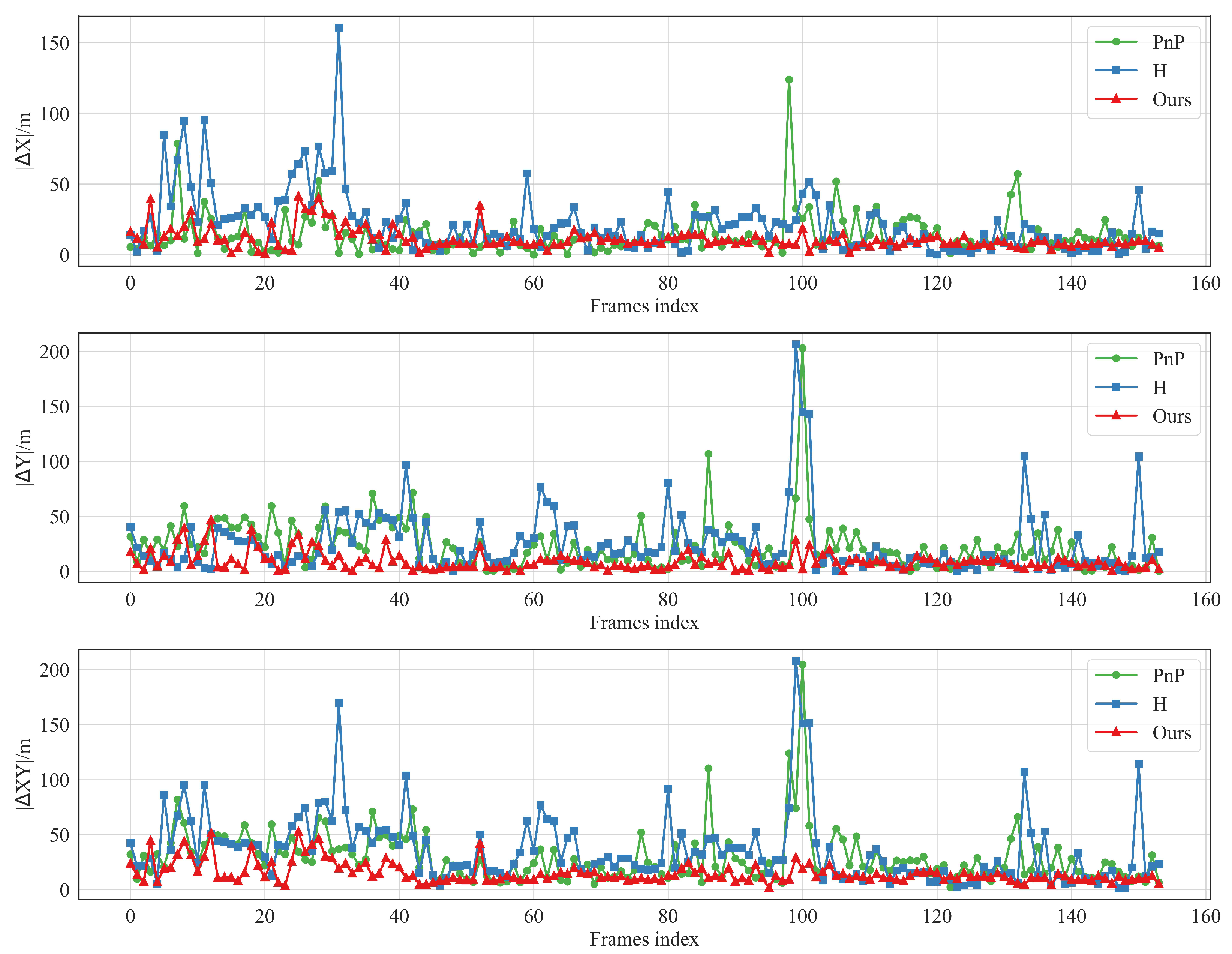
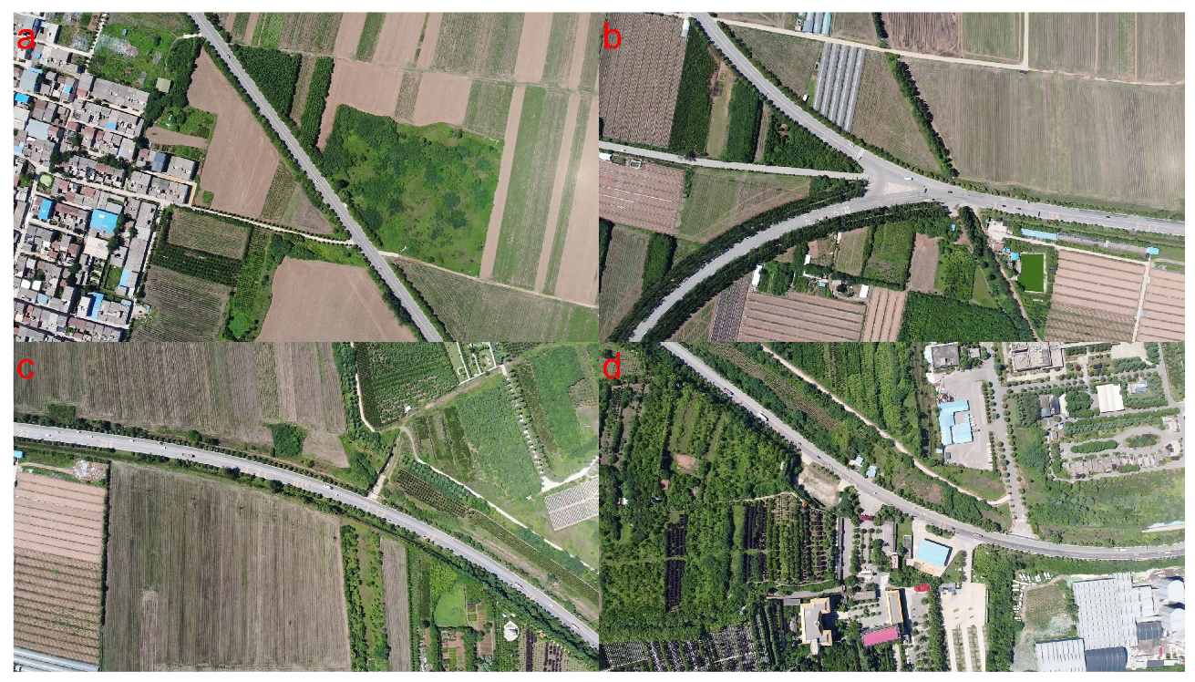
As shown in Figure 7, the localization error of the proposed method is compared with the other methods on the successfully localized sequence frames. From the overall graph trend, the algorithm proposed in this paper shows obvious advantages in terms of localization accuracy with lower error. The specific analysis is as follows: When the elevation information corresponding to the ground objects in the aerial image varies significantly, then the feature points exist at the same time points with significant elevation differences, such as tall buildings and the ground, e.g., frame 32,100 in Figure 8. Furthermore, methods based on PnP and the single-response matrix decomposition exhibit significant localization errors. This occurs because their planar assumption breaks down in scenes with substantial elevation variations, leading to inaccurate position estimation and thus larger localization errors. However, for those without significant elevation changes such as frame 79 and 95 in Figure 8, the localization errors of these methods are relatively small and the localization results are more accurate. In contrast, the methods proposed in this paper are more accurate for localization in different scenarios.

Figure 7.
Geolocalization errors of three methods. The subgraphs display errors across different dimensions, with the x-axis as frame index and y-axis as error values. PnP indicates the Perspective-n-Point for geolocation estimation. H denotes the homography matrix decomposition. Our method integrates relative depth info to boost geolocation accuracy estimation.

Figure 8.
Selected aerial image frames: (a) frame 32, (b) frame 100, (c) frame 79, and (d) frame 95.
Table 2 shows the statistical characteristics of the positioning errors of the three geolocalization methods. From the table, it can be seen that the maximum, mean, median, and standard deviation of the positioning errors of the proposed method are smaller than those of the other two methods, indicating that the proposed geolocalization method has high accuracy and stability.
Table 2.
Statistical characteristics of positioning errors of three geolocalization methods.
3.2.4. Ablation Experiments
To evaluate the effectiveness of the feature-matching pair screening strategy in the proposed method, we designed ablation experiments. We quantitatively analyzed the following two filtering strategies: one is the confidence filtering strategy, which filters the matched subsets by setting a reasonable confidence threshold to eliminate the subsets with low confidence to reduce their negative impact on the accuracy of the position estimation; and the other is the convex hull area ratio filtering strategy, which filters the size of the convex hull area constituted by the feature points. It preferentially retains the subset of matches with larger convex packet areas, aiming to optimize the spatial distribution uniformity of the matched pairs in the image and thus improve the stability and accuracy of the position estimation.
The experimental results are shown in Table 3, where “#Matched” denotes the number of matched pairs in the final matched subset, “✓” indicates that the strategy is selected, and “✕” indicates that it is not selected. The confidence filtering strategy demonstrates significant mismatch filtering ability, and the geolocalization error of 24.42 m is reduced to 19.63 m. This fully confirms the key role of this strategy in suppressing mismatch interference and improving the accuracy of the position-solving technique. The convex hull area filtering strategy, on the other hand, reduces the geolocalization error from 24.42 m to 18.52 m by optimizing the distribution quality of the matching points, which verifies its effectiveness in enhancing the spatial coverage uniformity of the matching points.
Table 3.
Effectiveness of average confidence and convex hull area ratio.
When the two strategies work synergistically, the geolocalization error of 24.42 m is reduced to 14.91 m compared to the scenario involving the application of a single strategy. This synergistic phenomenon indicates a complementary mechanism between confidence screening and convex hull area screening in the pose optimization process, with the former aimed at eliminating matching noise interference and the latter focused on improving the geometric distribution of matches. The experimental results confirm that combining the proposed screening strategy enhances geolocalization accuracy.
3.2.5. Parameter Experiments
In the geolocalization algorithm, the appropriate choice of parameters is pivotal for the algorithm’s efficacy. This section presents a comparative analysis that was conducted through fixed thresholds and dynamically selected thresholds. The average confidence threshold measures the reliability of feature-matching point pairs; conversely, the convex hull area ratio threshold evaluates the extent of discretization within the matching point set concerning spatial distribution. Guided by empirical experience, we systematically explored various threshold values. Specifically, was set at 0.4, 0.5, and 0.6, while was set at 0.2, 0.3, and 0.4. Subsequently, a cross experiment was executed.
The results of the parameter experiments are presented in Table 4, where recall indicates the ratio of successfully localized frames to the total number of frames. The table shows that a larger can enhance the reliability of the matching points; however, this may reduce the number of matching points that satisfy the specified conditions, consequently diminishing geolocalization accuracy and the percentage of successful localization frames due to a lack of reliable matching points. Conversely, a smaller will likely increase the proportion of false matching points within the subset, adversely affecting geolocalization accuracy. A larger will encourage a more uniform distribution of the matching points within the subgroup, yielding a more robust computation of the single-response matrix. Similarly, in specific scenarios, this may result in reduced subsets that meet the requirements and an increased likelihood of localization failure. A smaller , on the other hand, will lead to an overly concentrated distribution of the point set, implying that the spatial information of the matching points is not sufficiently wealthy and dispersed, which can result in issues such as numerical instability during the computation of the single-response matrix, thus affecting the accuracy and reliability of geolocalization. The dynamic threshold selection method proposed in this paper has the lowest geolocalization error and a recall rate of 88%, achieving a balance between geolocalization accuracy and success rate.
Table 4.
Comparison of experimental results under different parameters.
4. Discussion
Utilizing a real flight dataset, we meticulously designed and executed comparison, ablation, and parametric experiments to thoroughly assess the performance of the proposed method. The comparative results demonstrate that the proposed method significantly outperforms other approaches in terms of localization accuracy and stability. Furthermore, ablation studies validate the effectiveness of the confidence screening and convex envelope area screening techniques. These findings collectively demonstrate that integrating these two screening strategies significantly enhances localization accuracy. Conversely, the parametric experiments reveal that selecting the average confidence threshold and the convex hull area ratio threshold significantly influences localization performance. Merely increasing or decreasing a single threshold cannot optimize the geolocalization. Instead, finding a balance between them is key. The dynamic threshold selection strategy adopted in this paper can achieve a balance between geolocalization accuracy and geolocalization success rate, and has strong robustness.
5. Conclusions
In this paper, we propose an innovative approach, fusing 2D Earth observation imagery with relative depth information for aerial vehicle geolocalization. The process begins by inputting both aerial and reference satellite remote sensing images into a feature-matching network to extract pixel-level matching pairs. Next, a depth estimation network estimates the relative depth of features within the satellite image. Finally, high-confidence matching pairs with similar depths and uniform distribution are selected to estimate the aerial vehicle’s location. Experimental results confirm that this method surpasses existing geolocalization accuracy and stability. In future work, we plan to explore more advanced feature-matching and depth estimation networks to enhance the reliability of feature matching and the accuracy of depth information. Additionally, we plan to investigate the integration of inertial navigation data into our system.
Author Contributions
Conceptualization, M.Z. and D.Y.; methodology, M.Z., D.Y. and Y.L.; software, M.Z. and W.X.; validation, M.Z. and D.Y.; formal analysis, M.Z. and D.Y.; investigation, M.Z. and J.L.; resources, D.Y.; data curation, M.Z. and X.Q.; writing—original draft preparation, M.Z.; writing—review and editing, M.Z. and D.Y.; visualization, M.Z.; supervision, M.Z.; project administration, D.Y. and J.L.; funding acquisition, D.Y., Y.L. and J.L. All authors have read and agreed to the published version of the manuscript.
Funding
This paper is supported by the National Natural Science Foundation of China (Grant Nos. 42301535, 61673017, and 61403398).
Data Availability Statement
The data that have been used are confidential.
Conflicts of Interest
The authors declare no conflicts of interest.
References
- Maddikunta, P.K.R.; Hakak, S.; Alazab, M.; Bhattacharya, S.; Gadekallu, T.R.; Khan, W.Z.; Pham, Q.V. Unmanned aerial vehicles in smart agriculture: Applications, requirements, and challenges. IEEE Sens. J. 2021, 21, 17608–17619. [Google Scholar] [CrossRef]
- Sawadsitang, S.; Niyato, D.; Tan, P.S.; Wang, P.; Nutanong, S. Shipper cooperation in stochastic drone delivery: A dynamic Bayesian game approach. IEEE Trans. Veh. Technol. 2021, 70, 7437–7452. [Google Scholar] [CrossRef]
- Utsav, A.; Abhishek, A.; Suraj, P.; Badhai, R.K. An IoT based UAV network for military applications. In Proceedings of the 2021 Sixth International Conference on Wireless Communications, Signal Processing and Networking (WiSPNET), Chennai, India, 25–27 March 2021; pp. 122–125. [Google Scholar]
- Khan, A.; Gupta, S.; Gupta, S.K. Emerging UAV technology for disaster detection, mitigation, response, and preparedness. J. Field Robot. 2022, 39, 905–955. [Google Scholar] [CrossRef]
- Green, D.R.; Hagon, J.J.; Gómez, C.; Gregory, B.J. Using low-cost UAVs for environmental monitoring, mapping, and modelling: Examples from the coastal zone. In Coastal Management; Elsevier: Amsterdam, The Netherlands, 2019; pp. 465–501. [Google Scholar]
- Zheng, C.; Nie, J.; Yin, B.; Li, X.; Qian, Y.; Wei, Z. Frequency and Spatial-domain Saliency Network for Remote Sensing Cross-Modal Retrieval. IEEE Trans. Geosci. Remote Sens. 2025, 63, 5403313. [Google Scholar] [CrossRef]
- Das, S.; Sharma, R. A TextGCN-Based Decoding Approach for Improving Remote Sensing Image Captioning. IEEE Geosci. Remote Sens. Lett. 2024, 22, 8000405. [Google Scholar] [CrossRef]
- Unar, S.; Elhoseny, M.; Liu, P.; Su, Y.; Zhao, X.; Fu, X. Multicore feature learning approach for maximizing retrieval information in remote sensing images. IEEE Sens. J. 2023, 23, 27581–27589. [Google Scholar] [CrossRef]
- Yamani, B.; Medavarapu, N.; Rakesh, S. Remote Sensing Image Captioning Using Deep Learning. In Proceedings of the 2024 International Conference on Automation and Computation (AUTOCOM), Dehradun, India, 14–16 March 2024; pp. 295–302. [Google Scholar]
- Meng, X.; Guo, W.; Zhou, K.; Sun, T.; Deng, L.; Yu, S.; Feng, Y. AirGeoNet: A Map-Guided Visual Geo-Localization Approach for Aerial Vehicles. IEEE Trans. Geosci. Remote Sens. 2024, 62, 4707814. [Google Scholar] [CrossRef]
- Oquab, M.; Darcet, T.; Moutakanni, T.; Vo, H.; Szafraniec, M.; Khalidov, V.; Fernandez, P.; Haziza, D.; Massa, F.; El-Nouby, A.; et al. Dinov2: Learning robust visual features without supervision. arXiv 2023, arXiv:2304.07193. [Google Scholar]
- Jégou, H.; Douze, M.; Schmid, C.; Pérez, P. Aggregating local descriptors into a compact image representation. In Proceedings of the 2010 IEEE Computer Society Conference on Computer Vision and Pattern Recognition, San Francisco, CA, USA, 13–18 June 2010; pp. 3304–3311. [Google Scholar]
- Lowe, D.G. Object recognition from local scale-invariant features. In Proceedings of the Seventh IEEE International Conference on Computer Vision, Kerkyra, Greece, 20–27 September 1999; Volume 2, pp. 1150–1157. [Google Scholar]
- Bay, H.; Ess, A.; Tuytelaars, T.; Van Gool, L. Speeded-up robust features (SURF). Comput. Vis. Image Underst. 2008, 110, 346–359. [Google Scholar] [CrossRef]
- Rublee, E.; Rabaud, V.; Konolige, K.; Bradski, G. ORB: An efficient alternative to SIFT or SURF. In Proceedings of the 2011 International Conference on Computer Vision, Barcelona, Spain, 6–13 November 2011; pp. 2564–2571. [Google Scholar]
- Saleem, S.; Sablatnig, R. A robust SIFT descriptor for multispectral images. IEEE Signal Process. Lett. 2014, 21, 400–403. [Google Scholar] [CrossRef]
- Li, J.; Hu, Q.; Ai, M. RIFT: Multi-modal image matching based on radiation-variation insensitive feature transform. IEEE Trans. Image Process. 2019, 29, 3296–3310. [Google Scholar] [CrossRef] [PubMed]
- Han, X.; Leung, T.; Jia, Y.; Sukthankar, R.; Berg, A.C. Matchnet: Unifying feature and metric learning for patch-based matching. In Proceedings of the IEEE Conference on Computer Vision and Pattern Recognition, Boston, MA, USA, 7–12 June 2015; pp. 3279–3286. [Google Scholar]
- DeTone, D.; Malisiewicz, T.; Rabinovich, A. Superpoint: Self-supervised interest point detection and description. In Proceedings of the IEEE Conference on Computer Vision and Pattern Recognition Workshops, Salt Lake City, UT, USA, 18–23 June 2018; pp. 224–236. [Google Scholar]
- Sarlin, P.E.; DeTone, D.; Malisiewicz, T.; Rabinovich, A. Superglue: Learning feature matching with graph neural networks. In Proceedings of the IEEE/CVF Conference on Computer Vision and Pattern Recognition, Seattle, WA, USA, 13–19 June 2020; pp. 4938–4947. [Google Scholar]
- Lindenberger, P.; Sarlin, P.E.; Pollefeys, M. Lightglue: Local feature matching at light speed. In Proceedings of the IEEE/CVF International Conference on Computer Vision, Paris, France, 1–6 October 2023; pp. 17627–17638. [Google Scholar]
- Sun, J.; Shen, Z.; Wang, Y.; Bao, H.; Zhou, X. LoFTR: Detector-free local feature matching with transformers. In Proceedings of the IEEE/CVF Conference on Computer Vision and Pattern Recognition, Nashville, TN, USA, 20–25 June 2021; pp. 8922–8931. [Google Scholar]
- Wang, H.; Zhou, F.; Wu, Q. Accurate vision-enabled UAV location using feature-enhanced transformer-driven image matching. IEEE Trans. Instrum. Meas. 2024, 73, 5502511. [Google Scholar] [CrossRef]
- Yao, F.; Lan, C.; Wang, L.; Wan, H.; Gao, T.; Wei, Z. GNSS-denied geolocalization of UAVs using terrain-weighted constraint optimization. Int. J. Appl. Earth Obs. Geoinf. 2024, 135, 104277. [Google Scholar] [CrossRef]
- Lepetit, V.; Moreno-Noguer, F.; Fua, P. EP n P: An accurate O (n) solution to the P n P problem. Int. J. Comput. Vis. 2009, 81, 155–166. [Google Scholar] [CrossRef]
- Xu, W.; Yang, D.; Liu, J.; Li, Y.; Zhou, M. A Visual Navigation Algorithm for UAV Based on Visual-Geography Optimization. Drones 2024, 8, 313. [Google Scholar] [CrossRef]
- Qiu, X.; Liao, S.; Yang, D.; Li, Y.; Wang, S. High-precision visual geo-localization of UAV based on hierarchical localization. Expert Syst. Appl. 2025, 267, 126064. [Google Scholar] [CrossRef]
- Chen, Y.; Jiang, J. An oblique-robust absolute visual localization method for GPS-denied UAV with satellite imagery. IEEE Trans. Geosci. Remote Sens. 2023, 62, 5601713. [Google Scholar] [CrossRef]
- Li, Y.; Yang, D.; Wang, S.; Shi, L.; Meng, D. Geolocalization from Aerial Sensing Images Using Road Network Alignment. Remote Sens. 2024, 16, 482. [Google Scholar] [CrossRef]
- Yang, L.; Kang, B.; Huang, Z.; Zhao, Z.; Xu, X.; Feng, J.; Zhao, H. Depth anything v2. Adv. Neural Inf. Process. Syst. 2024, 37, 21875–21911. [Google Scholar]
- Yang, L.; Kang, B.; Huang, Z.; Xu, X.; Feng, J.; Zhao, H. Depth anything: Unleashing the power of large-scale unlabeled data. In Proceedings of the IEEE/CVF Conference on Computer Vision and Pattern Recognition, Seattle, WA, USA, 16–22 June 2024; pp. 10371–10381. [Google Scholar]
- Kneip, L.; Li, H.; Seo, Y. Upnp: An optimal o (n) solution to the absolute pose problem with universal applicability. In Proceedings of the Computer Vision–ECCV 2014: 13th European Conference, Zurich, Switzerland, 6–12 September 2014; Proceedings; Part I 13. Springer: Berlin/Heidelberg, Germany, 2014; pp. 127–142. [Google Scholar]
- Raguram, R.; Chum, O.; Pollefeys, M.; Matas, J.; Frahm, J.M. USAC: A universal framework for random sample consensus. IEEE Trans. Pattern Anal. Mach. Intell. 2012, 35, 2022–2038. [Google Scholar] [CrossRef] [PubMed]
Disclaimer/Publisher’s Note: The statements, opinions and data contained in all publications are solely those of the individual author(s) and contributor(s) and not of MDPI and/or the editor(s). MDPI and/or the editor(s) disclaim responsibility for any injury to people or property resulting from any ideas, methods, instructions or products referred to in the content. |
© 2025 by the authors. Licensee MDPI, Basel, Switzerland. This article is an open access article distributed under the terms and conditions of the Creative Commons Attribution (CC BY) license (https://creativecommons.org/licenses/by/4.0/).