Abstract
Dark ships, vessels deliberately disabling their AIS signals, constitute a grave maritime safety hazard, with detection efforts hindered by issues like over-reliance on AIS, inadequate surveillance coverage, and significant mismatch rates. This paper proposes an improved multi-feature association method that integrates satellite remote sensing and AIS data, with a focus on oriented bounding box course estimation, to improve the detection of dark ships and enhance maritime surveillance. Firstly, the oriented bounding box object detection model (YOLOv11n-OBB) is trained to break through the limitations of horizontal bounding box orientation representation. Secondly, by integrating position, dimensions (length and width), and course characteristics, we devise a joint cost function to evaluate the combined significance of multiple features. Subsequently, an advanced JVC global optimization algorithm is employed to ensure high-precision association in dense scenes. Finally, by integrating data from Gaofen-6 (optical) and Gaofen-3B (SAR) satellites, a day-and-night collaborative monitoring framework is constructed to address the blind spots of single-sensor monitoring during night-time or adverse weather conditions. Our results indicate that the detection model demonstrates a high average precision (AP50) of 0.986 on the optical dataset and 0.903 on the SAR dataset. The association accuracy of the multi-feature association algorithm is 91.74% in optical image and AIS data matching, and 91.33% in SAR image and AIS data matching. The association rate reaches 96.03% (optical) and 74.24% (SAR), respectively. This study provides an efficient technical tool for maritime safety regulation through multi-source data fusion and algorithm innovation.
1. Introduction
Dark ships specifically refer to those that actively shut down their Automatic Identification System (AIS) transmitters or consistently evade signal collection [1]. As a core subclass of non-cooperative vessels, their behavior patterns are significantly correlated with high-risk maritime illegal activities such as illegal fishing, drug smuggling, and piracy, which have become a key challenge in marine security supervision. According to global satellite observation data on ship activities [2], about 75% of industrial fishing vessels and 25% of merchant ships have long been outside the AIS monitoring network, creating large-scale regulatory blind spots. These dark ships not only exacerbate the exploitative development of marine resources but also provide covert channels for transnational crime by evading trajectory tracking, posing a core threat to maritime security governance. The current mainstream monitoring systems heavily rely on AIS data, yet their spatial coverage is limited and susceptible to interference from targeted counter-reconnaissance methods like equipment shutdowns and signal spoofing [3], making it difficult for traditional means such as shore-based radar and closed-circuit television (CCTV) to continuously track distant targets.
Confronting these challenges, satellite remote sensing technology, with its unique advantages in acquisition frequency, spatial resolution, and all-weather monitoring, has opened up new research directions for the detection of dark ships. The core of dark ship detection lies in identifying ship targets that lack AIS signals, and remote sensing images can accurately identify and locate different sizes of ship targets without being restricted by whether the AIS system is activated. In particular, SAR (Synthetic Aperture Radar) images have the capability to collect data under all weather conditions, day or night [4]. At the same time, satellite technology also offers the advantage of wide coverage, enabling large-scale detection of vessel targets [5]. However, satellite remote sensing lacks semantic information such as ship identity and type, while AIS data contains rich attributes but suffers from signal loss. By combining satellite remote sensing images with AIS data, information can be complemented and enhanced, forming a complete monitoring chain of “target detection-identity recognition” [6]. However, traditional methods for associating satellite remote sensing and AIS data still face two major bottlenecks: one is the matching error between remote sensing detection boxes and AIS data, which is caused by the ambiguity of horizontal box orientation. In particular, conventional horizontal bounding boxes are unable to account for the tilt or rotation of vessels, which leads to an inaccurate depiction of the vessel’s position, dimensions, and course characteristics. This inaccuracy can result in ambiguity when aligning remote sensing targets, as the tilt or rotation of the vessel is not taken into consideration, resulting in heading ambiguity when matching remote sensing targets with AIS trajectories; the second is the insufficient accuracy of association algorithms in dense scenarios. Currently, mainstream association algorithms, such as the nearest neighbor (NN) method, exhibit a notably higher mismatching rate in scenarios with high vessel density. This is attributed to their reliance on a single feature dimension, namely, position distance, which greatly hinders the efficacy of maritime supervision.
At present, researchers have widely used the method of associating satellite remote sensing images with AIS data, such as ship classification [7,8,9], dark ship detection [10,11,12], illegal fishing [13,14], and illegal oil discharge [15]. This is partly attributed to the ongoing enhancement of ship object detection accuracy. Since AlexNet [16] won the ImageNet image classification competition in 2012, deep learning has rapidly developed, and various ship object detection models have replaced classical machine learning classifiers like support vector machine [17], decision tree [18], and random forest [19], including two-stage models (Faster R-CNN [20], FPN [21]), single-stage models (YOLO [22], SSD [23]), and transformer-based detectors. Many scholars have proposed more advanced algorithms for ship target features and scenarios, such as the ADV-YOLO model [24], which introduces a SAR ship detection model based on improvements to YOLOv8, achieving an AP50-95 of 70% on the HRSID dataset [25]. YOLOShipTracker [26] introduces an improved SAR image ship detection and tracking method based on the lightweight YOLOv8n. Employing lightweight architecture and knowledge distillation techniques, it reduces computational complexity and enhances detection accuracy. Additionally, it designs a C-BIoU multi-objective tracking algorithm that enhances tracking stability through buffer area expansion and cascade matching strategies. MSDFF-Net [27] proposes a method for detecting ships in arbitrary directions of multi-scale unbalanced SAR images. The core of this method involves optimizing three modules: MSLK-Block (multi-scale large kernel convolution block) to enhance multi-scale feature extraction, DFF-Block (dynamic feature fusion block) to dynamically balance spatial and channel feature fusion, and GPD loss function (Gaussian probability distribution loss) to optimize regression tasks. On the other hand, there is continuous innovation of methods to associate satellite remote sensing images with AIS data. In the data association process, point-to-point associations are widely used [28]. Two sets of points were constructed: the first set includes the center of ship pixels detected in remote sensing images, and the second set contains ship positions from AIS data. Prior to extracting AIS data on ship positions, addressing the time discrepancy between sensor acquisitions is essential. Typically, linear interpolation [29] or spline interpolation [30] methods are used to extrapolate the AIS-reported positions to the time of remote sensing image acquisition. After achieving spatio-temporal alignment between the two datasets, the data association between remote sensing images and AIS in existing studies is mainly achieved through simple methods, such as nearest neighbor (NN) [31]. Nearest neighbor is a form of proximity search that assigns data based on the minimum distance, where “distance” is defined by a selected distance metric or threshold. The optimal method currently implemented is the global optimal association algorithm, such as the global nearest neighbor (GNN) [32], rank-ordered assignment [7], shape context-based point pattern matching (SC-PPM) [33], and moving ship optimal association (MSOA) [34].
The essence of global optimization algorithms lies in effectively addressing the allocation problem, which entails determining the minimum cost across all possible allocations. The value of the cost is generally calculated based on multiple attribute characteristics of the vessel target. However, the horizontal bounding boxes prevalent in current object detection algorithms exhibit directional ambiguity, frequently failing to precisely capture the course feature of the vessel, especially in dense scenes where vessel targets overlap. If the vessel’s direction does not align with the horizontal bounding box, the box’s size and position fail to accurately mirror its actual position and shape. Therefore, in dense shipping environments, data association is particularly challenging, and vessels detected in remote sensing images may be incorrectly associated with AIS observations, often leading to erroneous or inaccurate maritime monitoring results.
In view of the above problems, this paper proposes three innovative solutions:
- The oriented bounding box detection solves the problem of missing course characteristics. The oriented bounding box is constructed based on the YOLOv11-OBB model [35], and the ship’s heading angle is extracted using the long side definition method to break through the limitation of horizontal box orientation representation.
- The multi-feature joint cost function improves the association robustness. The joint cost function is constructed by integrating the position (longitude and latitude), dimensions (length and width), and course features, and global optimal matching in dense scenes is achieved using the improved JVC algorithm [36].
- Optical remote sensing (ORS) and SAR work together to break through the time blind area. The data of Gaofen-6 (optical) and GF-3B (SAR) satellites are combined to build a framework for day and night collaborative monitoring and datasets of ship targets so as to solve the problem of monitoring blind areas under night or severe weather conditions with a single sensor.
The organization of this paper is as follows. Section 2 introduces the ship detection algorithm, the AIS data processing workflow, and the association algorithm between remote sensing images and AIS. Section 3 explains the study area and data and presents the experimental results. Section 4 analyzes and discusses the experiments. Section 5 provides conclusions, identifies shortcomings, and offers suggestions for future work.
2. Methods
As shown in Figure 1, the workflow of this paper includes three stages. First, satellite remote sensing imagery and ship datasets are constructed to train and test the deep neural network model. At the same time, remote sensing images of the study area are acquired to use the trained model for ship detection. Subsequently, AIS data from the study area undergoes cleaning and spatio-temporal alignment. Finally, common features from remote sensing images and AIS are selected to calculate a multi-feature joint cost of position, dimensions, and course. The improved JVC algorithm is applied to determine the allocation with the minimum global cost, from which outcomes for dark ship detection are derived.
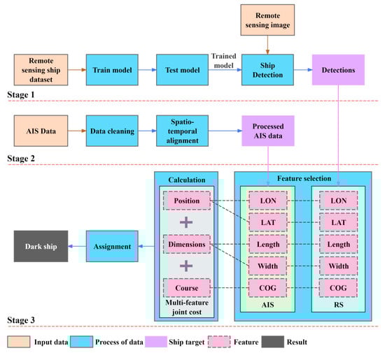
Figure 1.
Workflow for dark ship detection.
2.1. Ship Detection
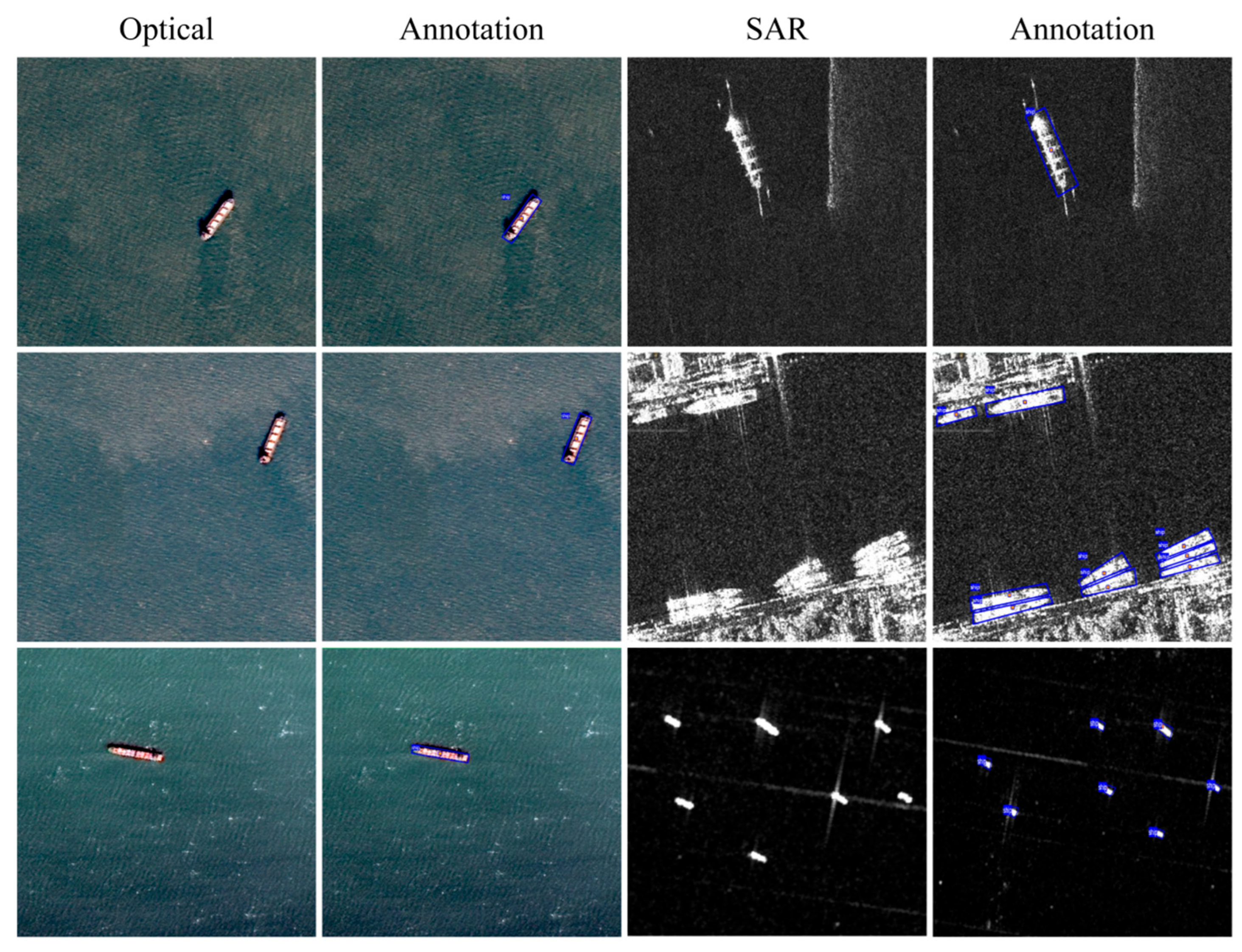
To train the convolutional neural network, we assemble datasets of maritime vessel targets from optical remote sensing and SAR images. The optical dataset, comprising 24 scenes of Gaofen-6 remote sensing images, was captured in the Bohai Sea region from 2023 to 2024. Each image was cropped to a resolution of 512 × 512 pixels, resulting in a total of 3092 images. These images include 3520 vessel entities, providing a comprehensive resource for monitoring and analysis in the region. These are annotated using roLabelImg 1.8.6 [37] with oriented bounding boxes. The training set (2473) and test set (619) are divided in an 8:2 ratio. The SAR dataset is composed of open-source datasets SSDD+ [38] and SRSDD [39], comprising 1826 images, including 5433 vessel entities. These are also annotated with oriented bounding boxes and divided into a training set (1460) and a test set (366) with an 8:2 ratio. Figure 2 shows examples of the two datasets.

Figure 2.
Examples of optical dataset and SAR dataset.
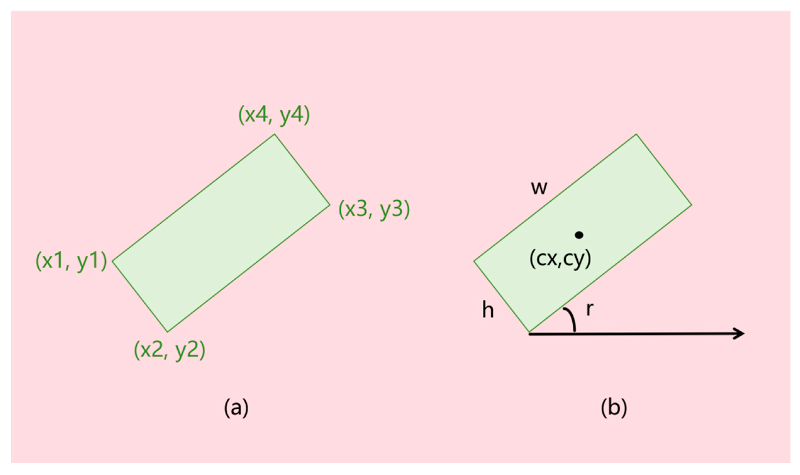
The YOLOv11 model [35] is used for ship detection. To guarantee real-time detection capability for dark ships, we selected the lightest YOLOv11-n model. Furthermore, we used the YOLOv11n-OBB model based on oriented bounding boxes (OBBs). Unlike traditional horizontal bounding boxes, OBBs can more accurately fit the actual shape of ships. This avoids errors caused by inconsistencies between ship orientation and horizontal bounding boxes when calculating ship position, dimensions, and course characteristics, thus providing a more precise foundation for subsequent data association. As shown in Figure 3, the YOLO-OBB format [40] defines the bounding box using four corner points, with coordinates normalized between 0 and 1, i.e., . It can be converted to the long-side definition format [41], where represents the center point coordinates of the target, and are the length and width of the ship, and is the angle between the long side and the horizontal axis. The angle between the ship and due north is then calculated using , resulting in the course (which may have a 180-degree ambiguity). This ultimately enables the extraction of features such as the ship’s longitude, latitude, length, width, and course.
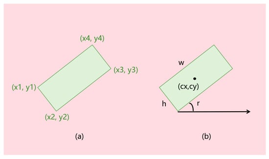
Figure 3.
The definition methods for OBB: the (a) YOLO-OBB definition method and (b) long-edge definition method.
The YOLOv11n-OBB model was trained on a computer equipped with the 9th generation Intel (R) Core (TM) i9-9900K @ 3.60GHz and NVIDIA GeForce RTX 2080 Ti GPU. In this work, the model was implemented on the Python 3.10 platform using Pytorch 2.3.1 and Torchvision 0.18.1 packages. Additionally, the AdamW optimizer was used for training the model. The optical and SAR datasets were used separately for training and testing the YOLOv11 neural network. The YOLOv11 model undergoes a rigorous training process, consisting of 200 epochs, leveraging the computational power of a single GPU, utilizing a batch size of 32, which has been shown to achieve good convergence and performance, and an initial learning rate of 0.002. All hyperparameters were initially set according to the default.yaml configuration recommended by Ultralytics, which is pre-set for medium data augmentation scenarios. Considering the characteristics of OBB tasks—such as more complex boundary box regression—the learning rate, weight decay, and other key parameters are adjusted. By testing and comparing the effects of different parameter combinations, the model with the best performance is selected.
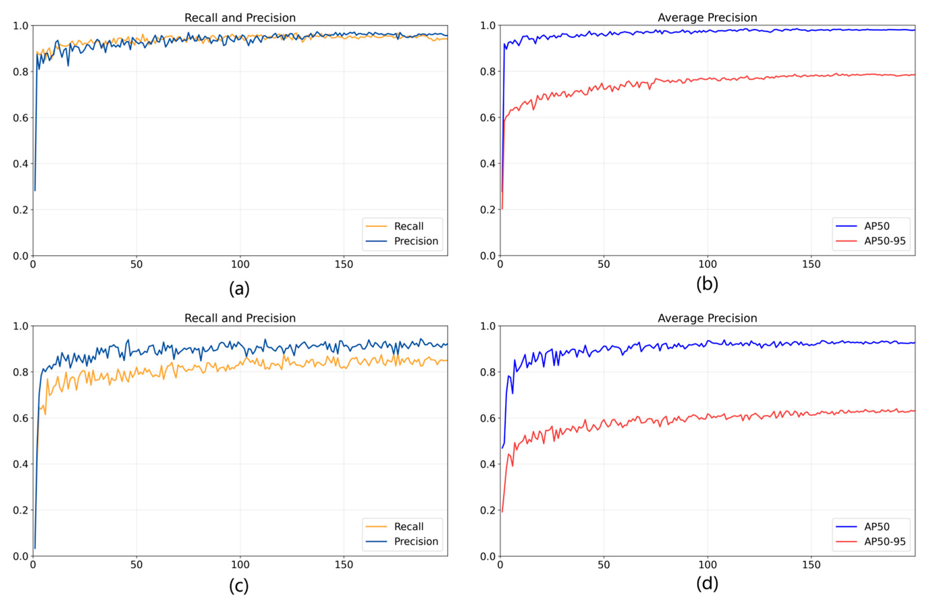
In the context of object detection, metrics such as precision, recall, AP50, AP50-95, and FPS are critical for assessing the performance of training outcomes. Equations (1)–(3) detail the calculation process of these metrics. Precision is the proportion of true positive samples among all predicted positive samples. Recall is the proportion of true positive samples among all positive samples. AP50 is the detection accuracy at an IoU threshold of 0.5, and AP50-95 is the average accuracy across different IoU values. The metrics of optical and SAR models (precision, recall, AP50, and AP50-95) with a change in training epochs are shown in Figure 4.

Figure 4.
The metrics of optical and SAR models with the change in training epoch. (a) Recall and precision of optical model. (b) AP50 and AP50-95 of optical model. (c) Recall and precision of SAR model. (d) AP50 and AP50-95 of SAR model.
To evaluate the performance of the YOLOv11n-OBB model, we conducted a comparative experiment with a target detection algorithm based on oriented bounding boxes. The experiments were conducted on both optical and SAR datasets, and the results are presented in Table 1. The YOLOv11n-OBB model shows the best performance on both data sets, followed by YOLOv8n-OBB, S2A-Net and ROI-Tansformer, with Oriented Faster-CNN performing the worst. Specifically, it achieves a test accuracy of 0.970, a recall rate of 0.968, and an AP50 of 0.986 on the optical dataset, showing robust performance despite challenges such as cloud interference. On the SAR dataset, although the test accuracy is slightly lower at 0.870, the recall rate and AP50 scores are 0.81 and 0.903, respectively, demonstrating its effectiveness in detecting ship targets in SAR images.

Table 1.
Comparison results of different detection algorithms based on oriented bounding boxes.
2.2. AIS Data Processing
Real-time AIS data transmission via radio signals ensures the provision of dynamic and static information about ships, which is pivotal for enhancing maritime navigation safety, managing traffic effectively, and conducting precise data analysis. Static information includes fixed attributes of the ship, such as name, MMSI (Maritime Mobile Service Identity), type, length, and width. Dynamic information consists of real-time navigation data, including timestamp, longitude, latitude, SOG (Speed Over Ground), COG (Course Over Ground), draft, destination port, and estimated time of arrival (ETA). Since the acquisition of AIS data involves processes like generation, encapsulation, transmission, reception, and decoding, ensuring no errors in the vast amount of raw data is challenging. Directly utilizing this data for analysis may interfere with the results; hence, preprocessing is necessary. We first clean the AIS data, with the following cleaning rules:
- Delete data where MMSI is not 9 digits. MMSI serves as the unique identification code for a vessel, with a standard format of 9 digits. The data may result from transmission errors, equipment failures, or human input mistakes. These erroneous data can interfere with subsequent vessel identification and analysis, so they need to be deleted.
- Remove data whose longitude is not in the range of [−180.0, 180.0] degrees.
- Remove data whose latitude is not in the range of [−90.0, 90.0] degrees.
- Delete data with SOG outside the range of [0, 51.2] knots.
- Delete data with COG outside the range of [0, 360] degrees.
In the process of organizing AIS data, information was segmented into distinct clusters based on MMSI, ensuring that each cluster represents a unique vessel. Within these clusters, the trajectory points were meticulously arranged in chronological order, culminating in a comprehensive dataset that captures the navigation patterns of individual ships over a specified timeframe. Next, AIS and remote sensing images were unified with the WGS-84 geographic coordinate system, with AIS data cropped to match the spatial range of the remote sensing images. Land masking was applied to AIS data to remove false alarms on land. Subsequently, AIS data was filtered into a time interval centered around the imaging start time of the remote sensing image, facilitating interpolation processing. The AIS data was interpolated using cubic spline interpolation to determine the position (latitude and longitude) of the ship at the moment of satellite remote sensing image acquisition, as well as the SOG and COG. For trajectory data that did not meet the boundary conditions of the cubic spline interpolation method, we used linear interpolation or kept it as it is (when the trajectory contains only one point). Finally, the points closest to the imaging time of the remote sensing image were extracted from the interpolated trajectory.
2.3. Data Association
The processes of associating remote sensing images with AIS data are as follows.
- Feature selection. The common features of remote sensing images and AIS were selected for subsequent calculation. In this paper, the position (longitude and latitude), dimensions (length and width), and course features are used.
- Calculate the multi-feature joint cost of position, dimensions, and course for remote sensing images and AIS data. The function for calculating the joint value is shown in Equation (4).In Equation (4), α represents the feature similarity between remote sensing images and AIS data, with a value ranging from 0 to 1. The closer it is to 1, the more similar the features are, and the lower the joint matching cost. Equation (5) provides the calculation formula for α. λ is the feature weight value, reflecting the relative importance of each feature in the joint cost calculation, and its values must satisfy Equation (6), which states that the sum of all weights equals 1, ensuring that each feature has a reasonable proportion in the joint cost calculation. In practical applications, the λ values of each feature are determined through sensitivity analysis (Section 4.2). In Equation (5), represents the Euclidean distance between the corresponding ship target features in remote sensing images and AIS data, and μ represents the threshold for the corresponding feature distance. The final result is an N × M cost matrix, where N is the number of ships extracted from remote sensing images, and M is the number of AIS ships.
- The optimal allocation result is obtained by using the improved JVC algorithm. The research shows that the algorithm is better than the auction algorithm variant in all cases [36]. On the premise of minimizing the global total cost, N ships from remote sensing images match the corresponding AIS information.
- Determine whether the cost of each remote sensing image ship target association result is less than the threshold.
- Output results. If less than the threshold, the association is successful; if greater than the threshold, the association fails. After data association between remote sensing images of ship targets and AIS data, three outcomes can be obtained. The first is when the remote sensing image and AIS successfully associate, indicating that the vessel is navigating normally. The second is when the remote sensing ship target exists but does not match the corresponding AIS signal, which means the vessel is a dark ship that needs monitoring. The last is that AIS signals exist, but the ship is not detected in remote sensing images. This may be caused by false-alarm AIS data or low-resolution remote sensing images.
3. Results
3.1. Study Area
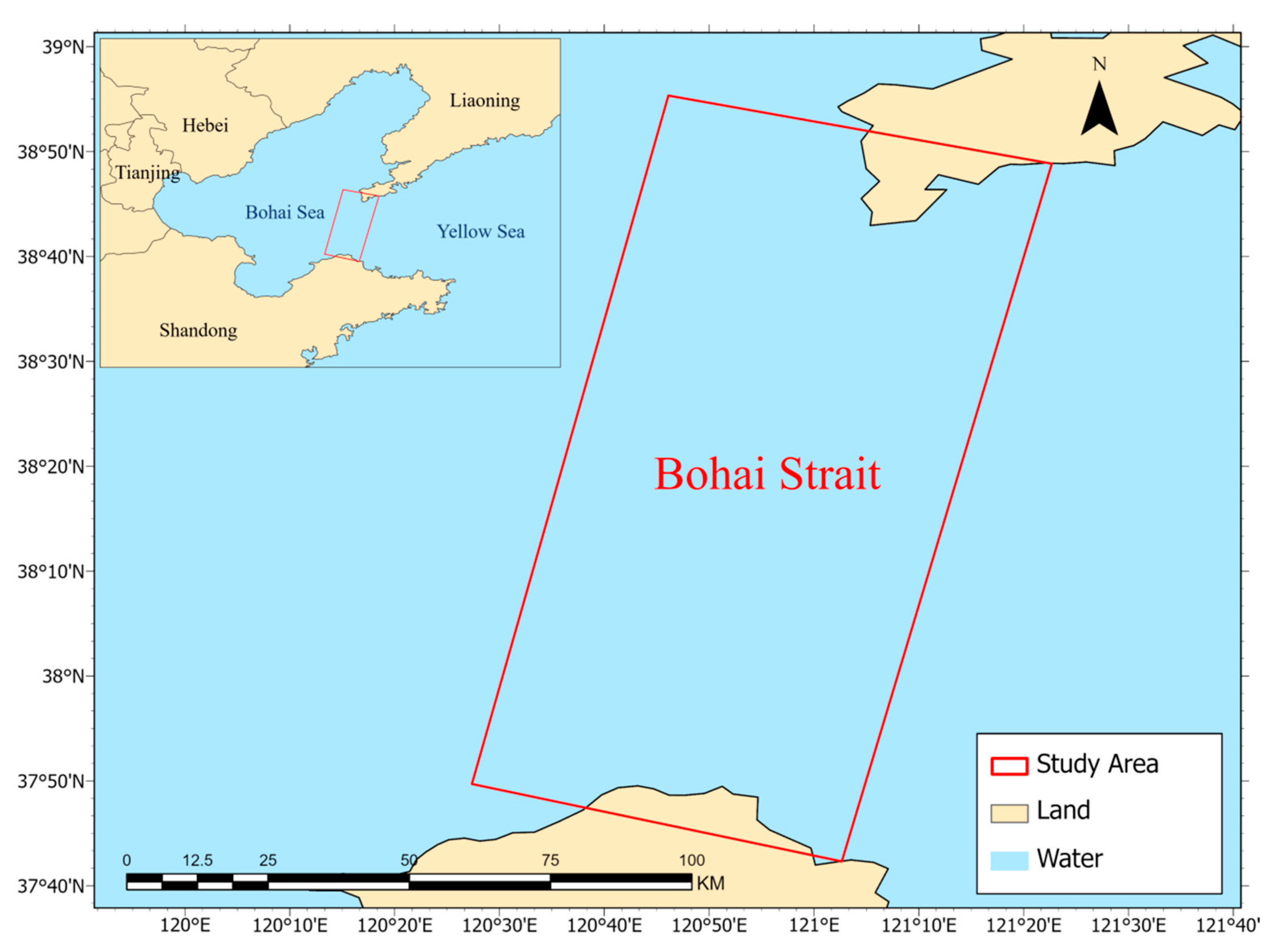
As shown in Figure 5, the study area is located between Laotieshan Cape at the southern end of Dalian City, Liaoning Province, China, and the Shandong Peninsula in Shandong Province. The Bohai Strait connects the Yellow Sea and the Bohai Sea, serving as the only outlet to the Bohai Sea. It is only 105 km wide from north to south; hence, it is known as the “Throat of the Bohai.” The community economy and marine economic development in the Bohai Rim region is advanced. The Bohai Rim area includes the Liaodong Peninsula Economic Zone, the Beijing–Tianjin–Hebei Economic Zone, and the Shandong Peninsula Blue Economy Zone, rendering it a pivotal economic development hub in China. The Bohai Sea boasts abundant fishery and mineral resources, featuring dense port networks and sophisticated maritime transport systems. It stands as a crucial maritime corridor for North China’s international commerce. The Laotieshan Channel on the northwest side of the strait serves as an international waterway, involving shipping interests of five countries: China, North Korea, Japan, South Korea, and Russia, with a massive volume of vessel traffic. As a vital maritime chokepoint and shipping hub in Northern China, the efficiency of the Bohai Strait’s vessel supervision system is crucial for safeguarding national maritime rights and interests and for fostering regional economic growth. The system’s effectiveness is particularly significant given the strategic importance of the strait and the high volume of maritime traffic it handles.
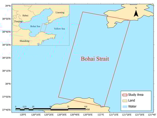
Figure 5.
Study area.
3.2. Optical Case
3.2.1. Data
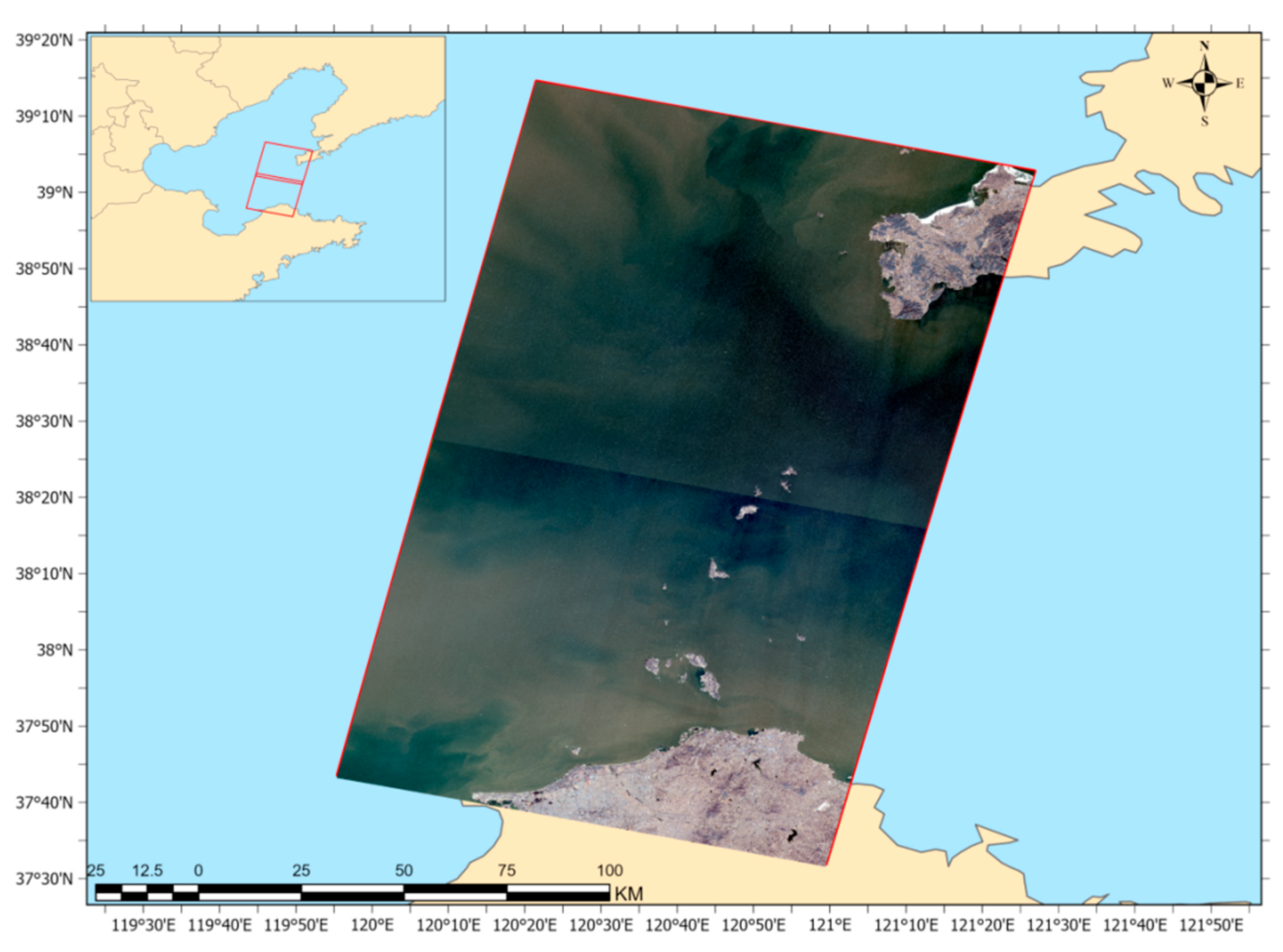
The multi-feature association method between satellite remote sensing and AIS data was tested on two optical remote sensing images of the Bohai Strait in China collected by the Gaofen-6 (GF-6) satellite. The optical remote sensing image’s preview appears in Figure 6, with comprehensive details outlined in Table 2. Gaofen-6 is equipped with high-resolution cameras with a panchromatic resolution of 2 m, a multi-spectral resolution of 8 m, and a swath width of 95 km [44]. The images were acquired at 10:57 a.m. on 6 March 2024, China Standard Time (CST). Preprocessing was performed before testing, including atmospheric correction, geometric correction, and image fusion. Additionally, AIS data from 10:30 a.m. to 11:30 a.m. on 6 March 2024 (CST) were obtained, totaling 114,027 records. The AIS data was provided by the Northern Navigation Service Center, Maritime Safety Administration, People’s Republic of China.
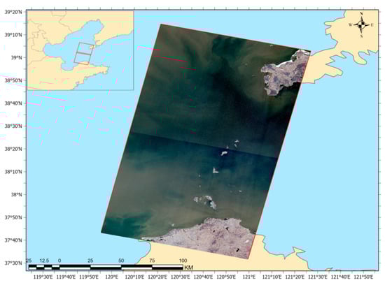
Figure 6.
Bohai Strait optical remote sensing data.
Table 2.
ORS product details.
3.2.2. Ship Detection
The model trained in Section 2.1 was used for ship detection. The YOLOv11 detection results were processed through land masking (including a 250 m buffer) to remove false alarms on land, ultimately returning 142 detection results in the optical image, as shown in Table 3. After manual verification, 26 detection results were identified as false alarms, and there were 10 missed detections. The majority of these false alarms originated from offshore drilling platforms and wind power facilities, which were subsequently removed via manual intervention. Finally, there were 126 ship targets on images in total.
Table 3.
Results of ORS image ship detection.
3.2.3. AIS Data Processing
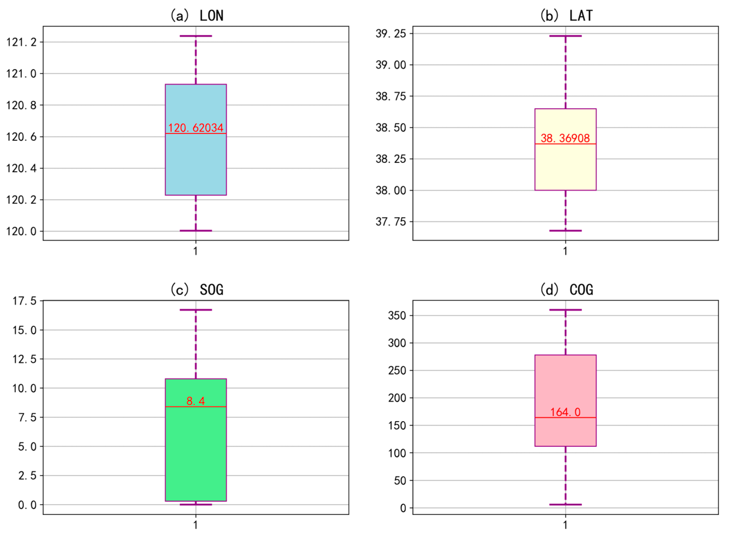
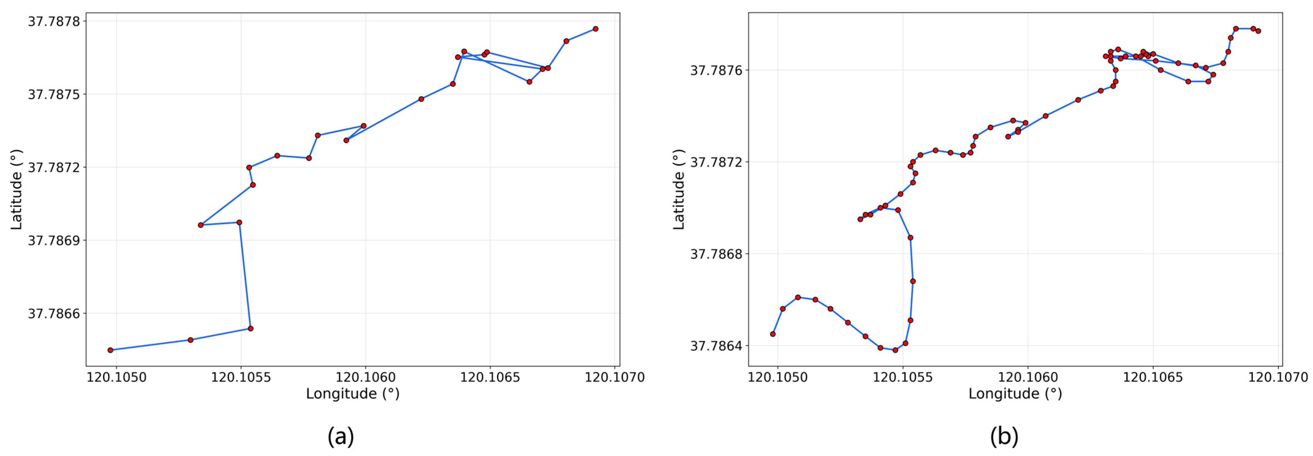
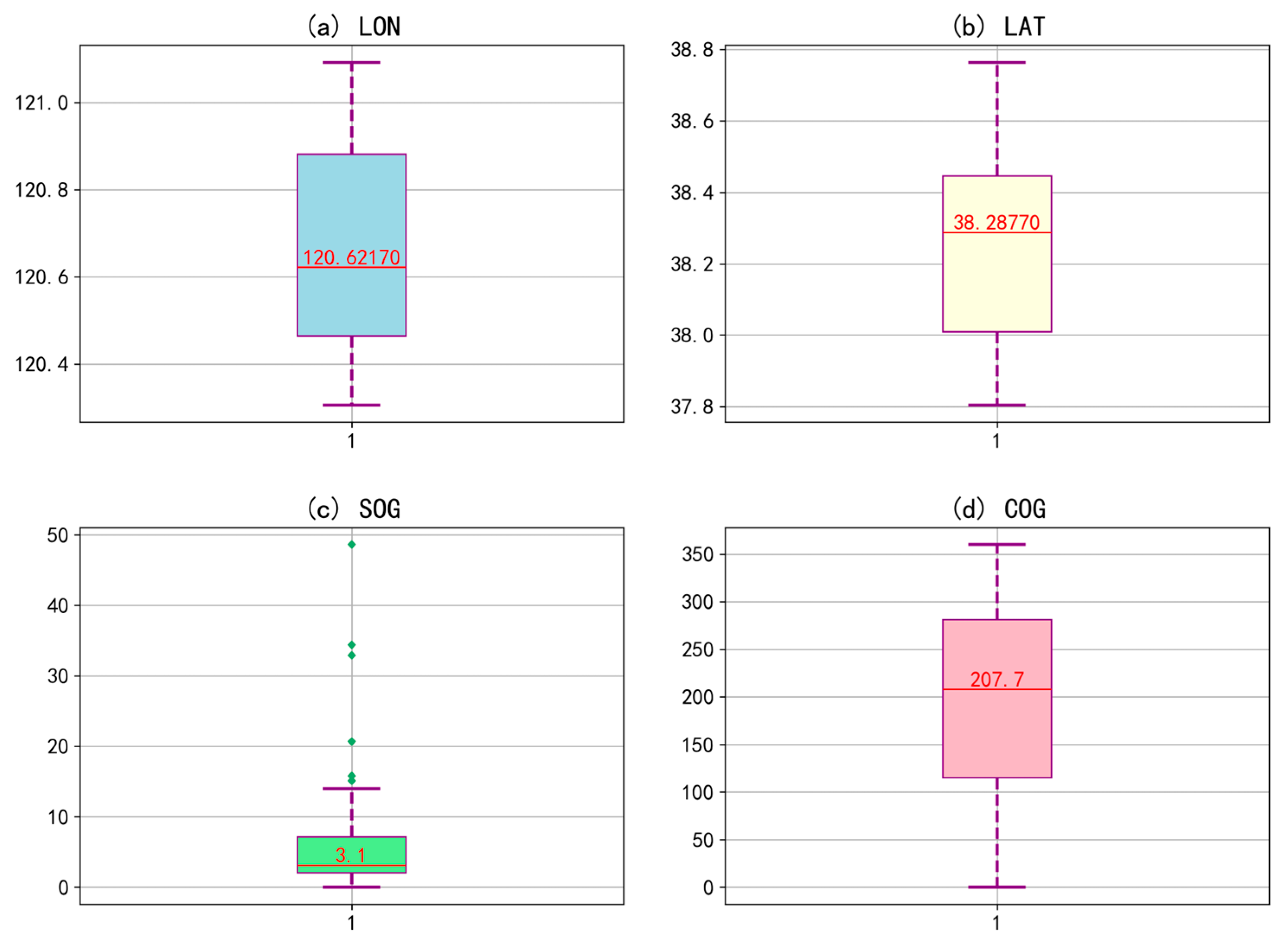
The AIS data associated with detection in optical images follows the process described in Section 2.2. For time filtering, a 60 min interval was chosen, meaning that AIS data from 10:30 to 11:30 (CST) on 6 March 2024 were considered for association. Following spatial filtering and the application of cubic spline interpolation, we successfully identify a total of 161 vessels, each with a unique MMSI number. Figure 7 shows the AIS statistical information for these 161 vessels, with the red line representing the median. The speed was primarily within 10 knots, and the heading was mainly southward. Figure 8 illustrates an example of cubic spline interpolation, where 144 vessels (89.4%) were successfully interpolated to a time interval of less than 10 s from the remote sensing image acquisition time.

Figure 7.
Statistical information of AIS data in optical case: (a) LON, (b) LAT, (c) SOG, and (d) COG.
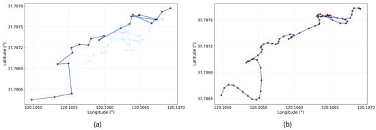
Figure 8.
Example of AIS trajectory: (a) original data; (b) cubic spline interpolation.
3.2.4. Data Association
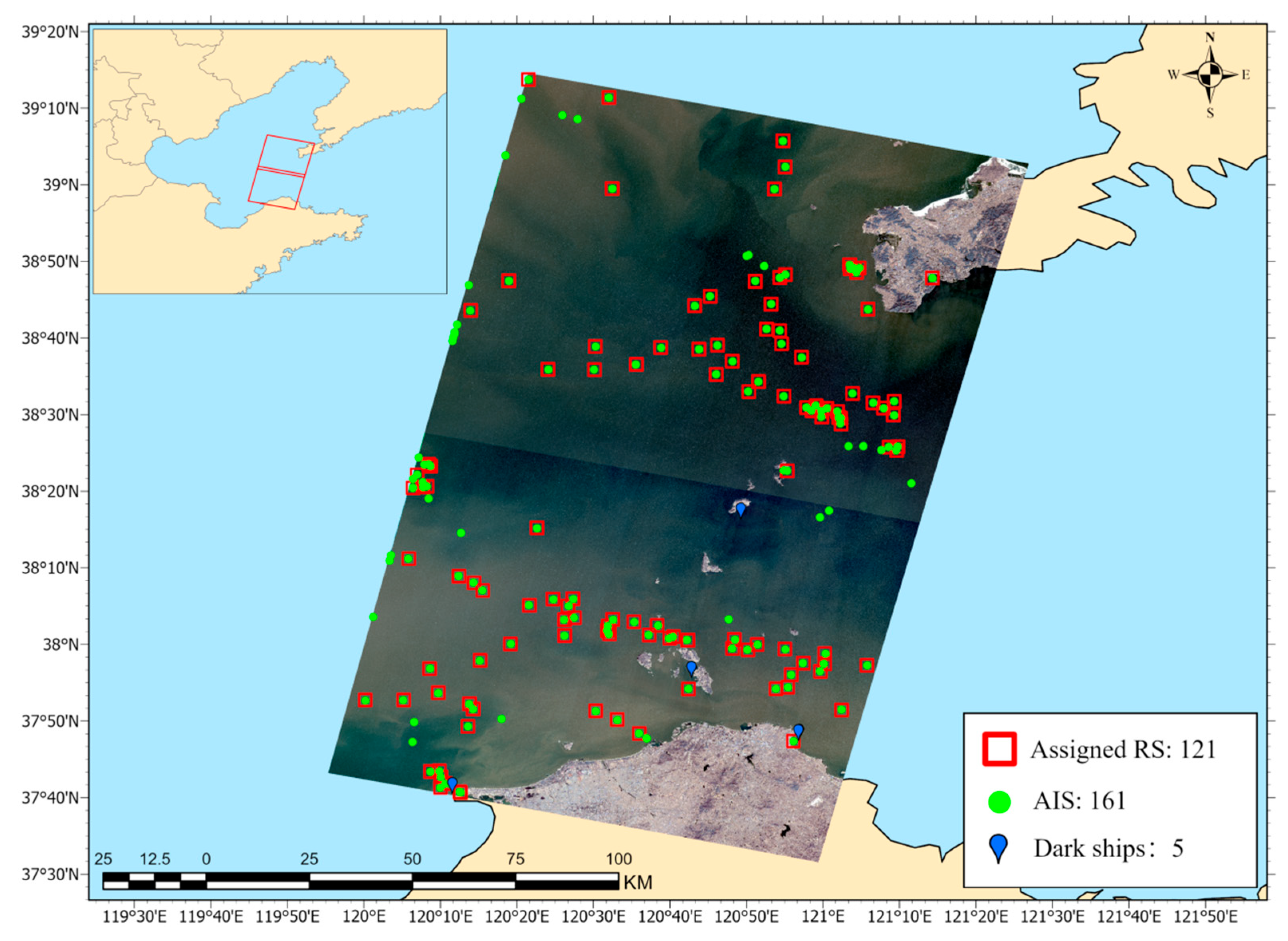
Table 4 provides the total number of optical imagery vessel targets and AIS data points, as well as the number of successful and failed associations for each. Among these, there are five vessels not associated with AIS on the optical remote sensing images (i.e., dark ships). In total, 121 vessels are successfully associated, accounting for 96.03% of the optical imagery vessels (126) and 75.16% of the AIS data points (161).
Table 4.
Results of ORS and AIS association.
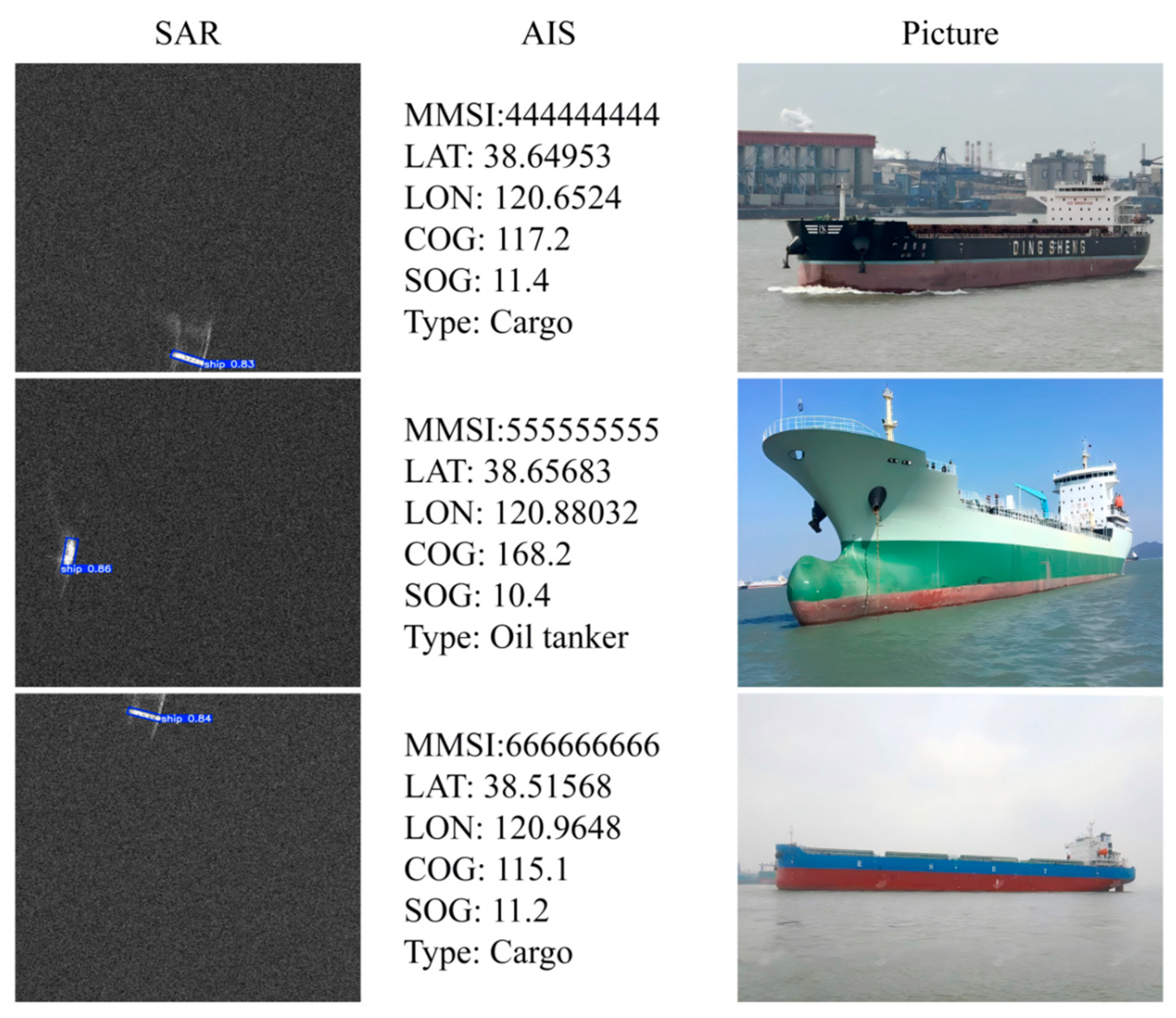
Figure 9 shows an example of three ships that are successfully associated. In order to protect the privacy of the ships, the MMSI of each ship in the final result is replaced with a random number. The ship name is not displayed; only the ship type is retained. Figure 10 shows the monitoring results of dark ships based on ORS and AIS data association.
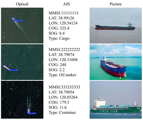
Figure 9.
Examples of assigned ships in optical case.
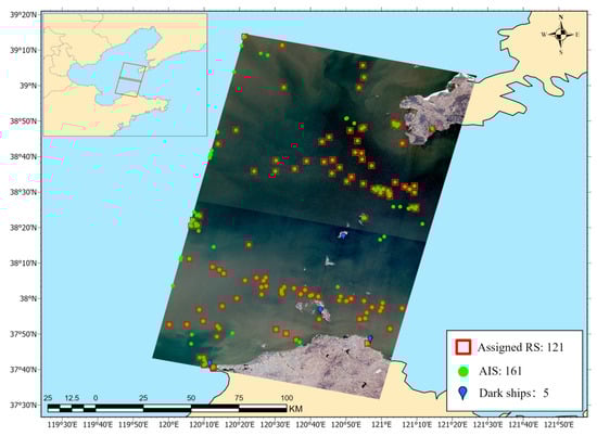
Figure 10.
Results of dark ship detection in the Bohai Strait based on ORS and AIS data association.
3.3. SAR Case
3.3.1. Data
The SAR case tests two SAR images of the Bohai Strait in China collected by GF-3B satellites. The Gaofen-3 (GF-3) series of satellites is China’s first C-band multi-polarization synthetic aperture radar (SAR) satellite series with a resolution of 1 m. Its C-band radar combines penetration and high precision, capable of penetrating vegetation, clouds, and smoke, supporting all-weather, all-time observation [44]. The preview of the SAR products is shown in Figure 11, with detailed information provided in Table 5. The imaging mode is Fine Strip 1 (Fine Stripmap 1, FSI), with a resolution of 5 m and a polarization mode of HHHV, covering an amplitude width of 50 km. The images were acquired at 06:08 a.m. on 31 October 2024 (CST). Additionally, AIS data from 05:30 a.m. to 06:30 a.m. on 31 October 2024 (CST) are obtained, totaling 168,719 records.
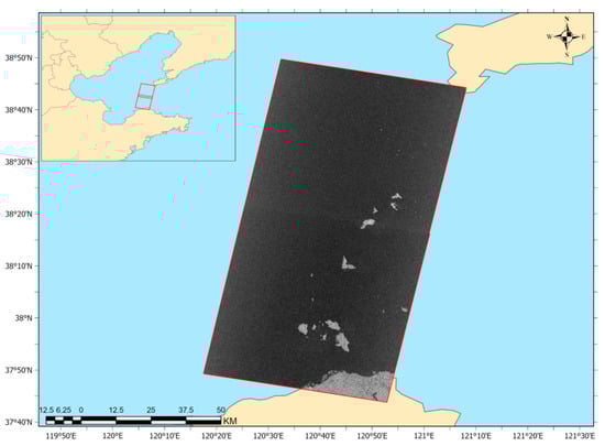
Figure 11.
Bohai Strait SAR products.
Table 5.
SAR product details.
3.3.2. Ship Detection
The model trained in Section 2.1 is used for ship detection. The YOLOv11 detection results are processed through land masking (including a 250 m buffer) to remove false alarms on land, ultimately returning 208 detection results in the SAR image, as shown in Table 6. After manual verification, 30 detection results were identified as false alarms, most of which originated from offshore wind power facilities and sea wave noise, and these false alarms were subsequently removed manually. There were 86 missed detections, primarily due to the resolution limitations of the SAR image. Of the missed targets, 79 were small vessels under 50 m (fewer than 10 pixels), making up 91.9% of the total, mainly fishing boats (62) and speedboats (4). In total, there were 264 ship targets on the SAR images.
Table 6.
Results of SAR image ship detection.
3.3.3. AIS Data Processing
The AIS data associated with the detection in SAR images follows the process described in Section 2.2. For time filtering, a 60 min interval was chosen, meaning that AIS data from 05:30 to 06:30 (CST) in October were considered for association. Following the application of spatial filtering and cubic spline interpolation techniques, a dataset comprising 464 unique vessels identified by their MMSI numbers was compiled. Of these, 374 vessels (80.6%) were successfully interpolated to the time interval less than 10 s from SAR imaging, demonstrating the effectiveness of the interpolation method. Figure 12 shows the AIS statistical information of these 464 vessels, with the red line representing the median. The speed is mainly within 10 knots, and the heading is predominantly south.

Figure 12.
Statistical information of AIS data in SAR case: (a) LON, (b) LAT, (c) SOG, and (d) COG.
3.3.4. Data Association
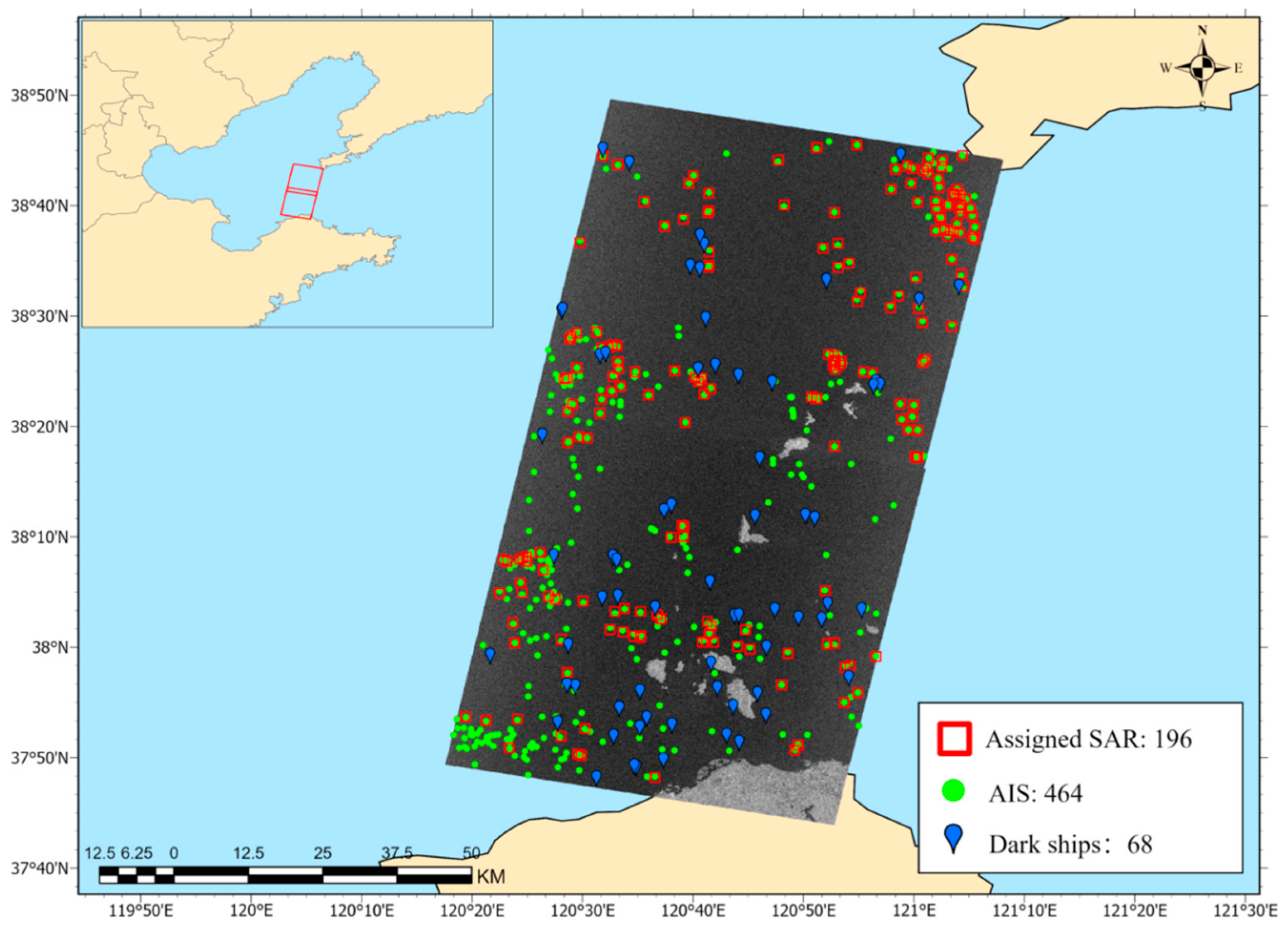
Table 7 shows the total number of ship detections in SAR imagery and AIS data points, as well as the number of their assignments and unassignments, among which there are 68 dark ships. A total of 196 ships were successfully associated, accounting for 74.24% of the ships in SAR images and 42.24% of the AIS data points.
Table 7.
Results of SAR and AIS association.
Figure 13 shows an example of three ships that were successfully associated. In order to protect the privacy of the ships, the MMSI of each ship in the final result was replaced with a random number. The ship name is not displayed; only the ship type is retained. Figure 14 shows the monitoring results of dark ships based on SAR and AIS data association.

Figure 13.
Examples of assigned ships in SAR case.

Figure 14.
Results of dark ship detection in the Bohai Strait based on SAR and AIS data association.
4. Discussion
4.1. Effectiveness of Data Association Methods Based on Multiple Features
To evaluate the performance of the multi-feature-based satellite remote sensing and AIS data association method, we used the following parameters to measure the point track association algorithm. First is the association rate, which is used to assess the applicability of the algorithm and the correlation analysis of the data. It is defined as the ratio of the number of associated points to the maximum number of points that can be associated, as shown in Equation (7). Here, represents the number of associated points, and represents the maximum number of points that can be associated between satellite remote sensing and AIS data. Second is the association accuracy, which evaluates the precision of the association algorithm. This is defined as the ratio of the number of correctly associated points to the total number of associated points, as shown in Equation (8). Here, represents the number of correctly associated points.
In order to verify the effectiveness of the multi-feature-based satellite remote sensing and AIS data association method, we carried out a comparative experiment with the nearest neighbor method (NN), rank-ordered assignment, and moving ship optimal association (MSOA). The results are shown in Table 8. The data preprocessing of all methods is consistent with the data association method based on multiple features. The experimental results show that the data association method based on multiple features has the optimal association rate and association accuracy in the optical case, followed by the MSOA algorithm, which effectively improves the association rate by 4.76% and the association accuracy by 3.04%. In the SAR case, the association rate of the data association method based on multiple features is slightly lower than that of MSOA algorithm, but its association accuracy reaches 91.33%, which is the best among all algorithms. Additionally, compared to the optical case, the multi-feature-based data association method demonstrates superior performance in improving the association accuracy in SAR case. This occurs because ship targets in SAR case are more densely concentrated, facilitating incorrect associations with the nearest neighbor method between ships detected in remote sensing images and AIS observations in heavily trafficked areas. Therefore, the multi-feature data association method proposed in this paper can effectively reduce the error rate of data association. This significant reduction in misalignment is of great importance in actual maritime monitoring scenarios. For example, in densely trafficked waters, it can effectively reduce the misidentification of ship identities caused by incorrect associations, avoiding regulatory errors due to erroneous ship information. This enhances the accuracy and safety of maritime traffic management, providing more reliable support for combating illegal vessel activities.
Table 8.
Association results for different methods.
4.2. Feature Sensitivity Analysis
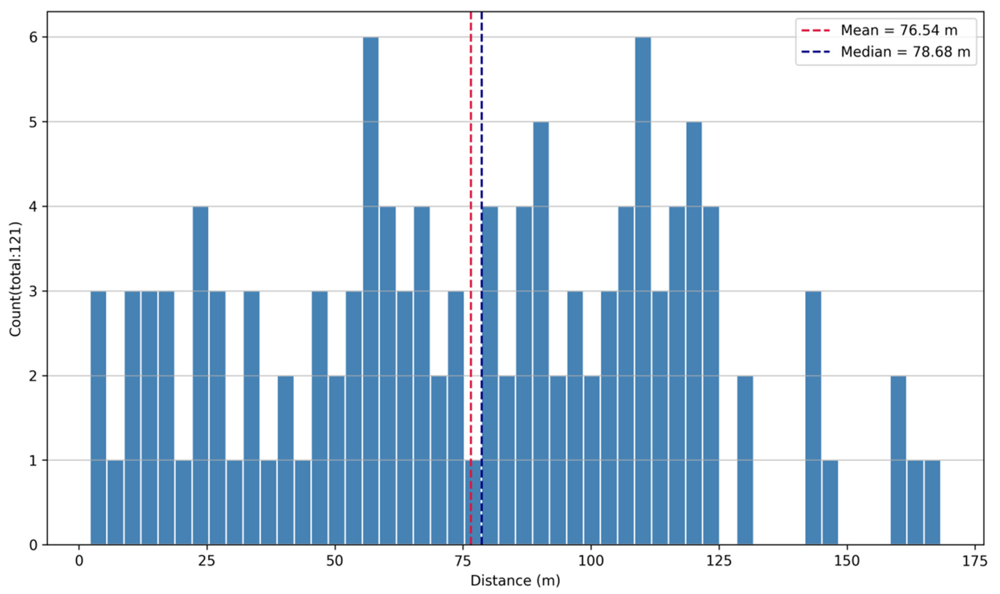
To determine the weight values of different features in this method, sensitivity analysis experiments were conducted on each feature based on the association results. Figure 15 shows the distribution of assignment distances in the optical case, with an average matching distance of 76.54 m. We can observe that half of the target matches have a matching distance less than 80 m. In our experiment, we set the distance threshold between the ship targets in remote sensing images and AIS positions to 500 m. This indicates a high degree of consistency between the ship positions estimated using optical remote sensing images and those reported by AIS. The number of targets with a matching distance exceeding 125 m is very low, less than 10% of the total number of targets. These targets are related to AIS messages that could not be accurately interpolated at the time of optical remote sensing image acquisition—for example, only a sparse number of AIS messages were available before or after the image acquisition time.

Figure 15.
Distribution of assignment distances in optical case.
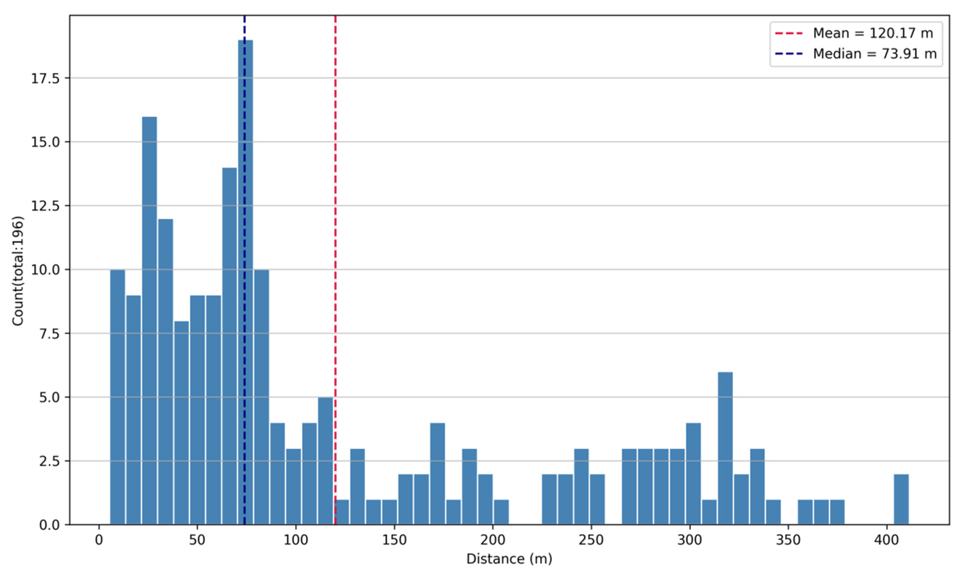
Figure 16 illustrates the distribution of assignment distances in a SAR case study, indicating an average match distance of 120.17 m, which is a critical metric for assessing the precision of the SAR’s distance measurement capabilities. Similarly, half of the SAR-AIS targets have a match distance less than 80 m, indicating a high degree of consistency. In comparison to the optical case, more targets have a match distance exceeding 100 m, with 21 targets (10.7%) having a match distance over 300 m. The inaccuracies in the SAR-AIS matching process can be attributed not only to the inability of AIS data to be accurately interpolated but also to the impact of SAR Doppler frequency shifts on moving vessels, causing the SAR targets to shift from their original positions [45]. For example, a vessel moving at about 15 knots might shift by approximately 700 m [32].

Figure 16.
Distribution of assignment distances in SAR case.
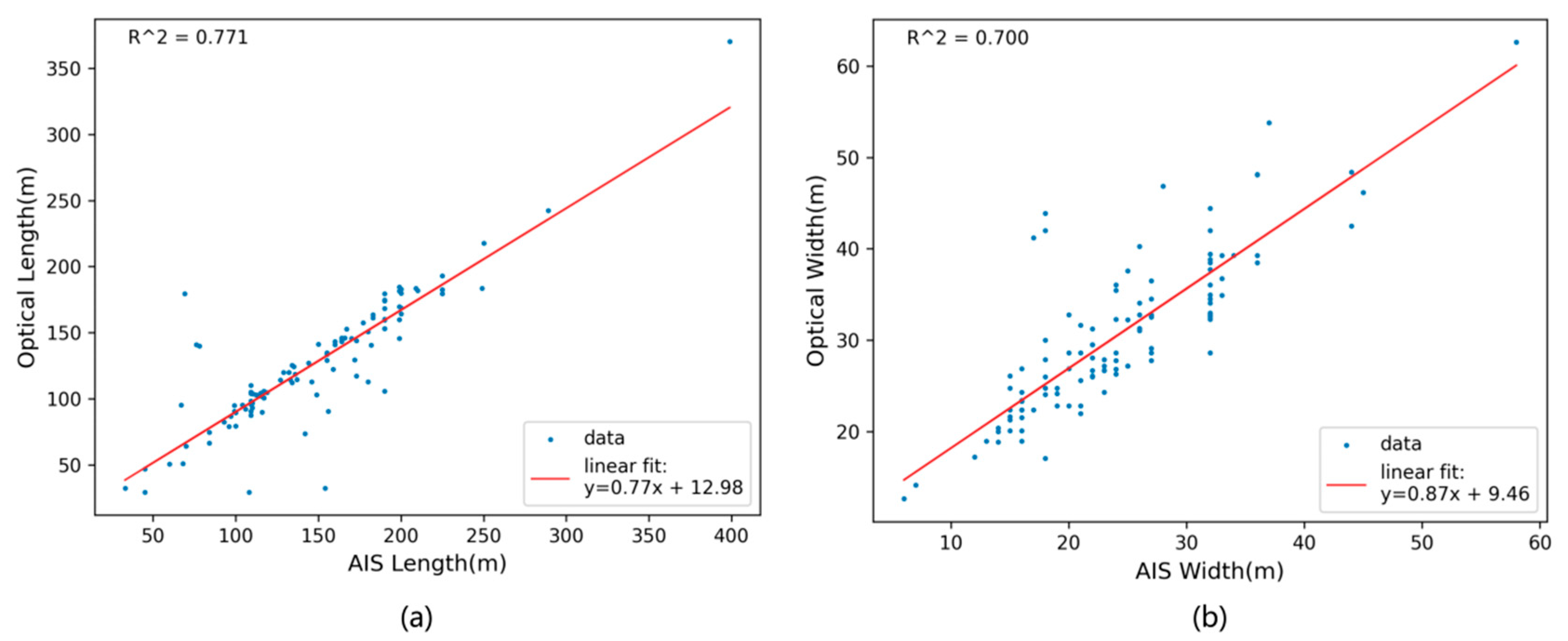
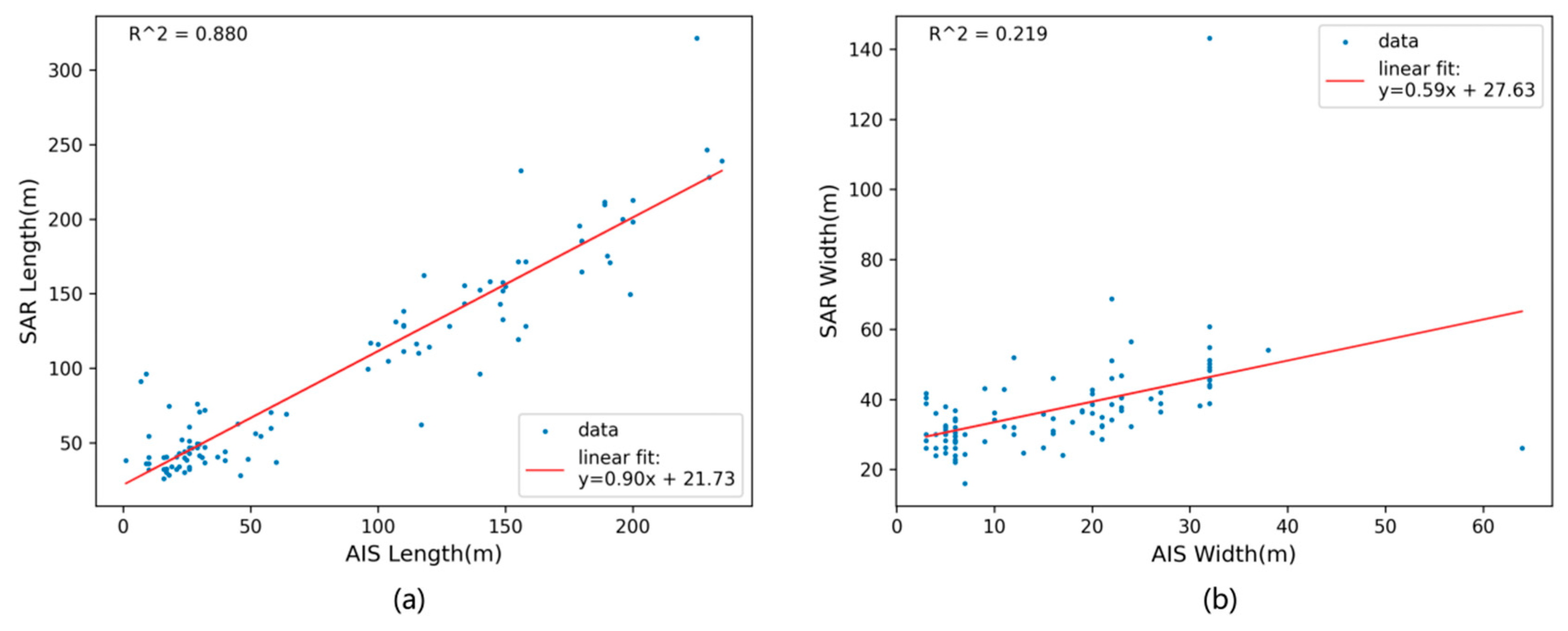
Figure 17a illustrates the correlation between the estimated ship length returned by the YOLOv11-OBB algorithm and the reported AIS length for each match value. Figure 17b illustrates a similar graph with vessel width data. The lengths and widths estimated from optical remote sensing images show a high degree of consistency with those reported by AIS. Figure 18 illustrates the relationship between the estimated ship length and width in SAR cases and their associated AIS length and width. There is a high degree of consistency in length, but for most AIS-reported widths, there is an overestimation. This overestimation may be due to SAR azimuth ambiguity. Due to target motion (rotation and acceleration), SAR imaging can cause target blurring in the azimuth direction, with blurring up to 100 m [46]. Additionally, the low resolution of SAR leads to greater estimation errors for ship width, especially for small targets. Therefore, we chose to reduce the weight of the width feature during association to improve the accuracy of the association.

Figure 17.
Estimated optical (a) length and (b) width against reported AIS.
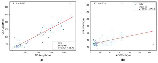
Figure 18.
Estimated SAR (a) length and (b) width against reported AIS.
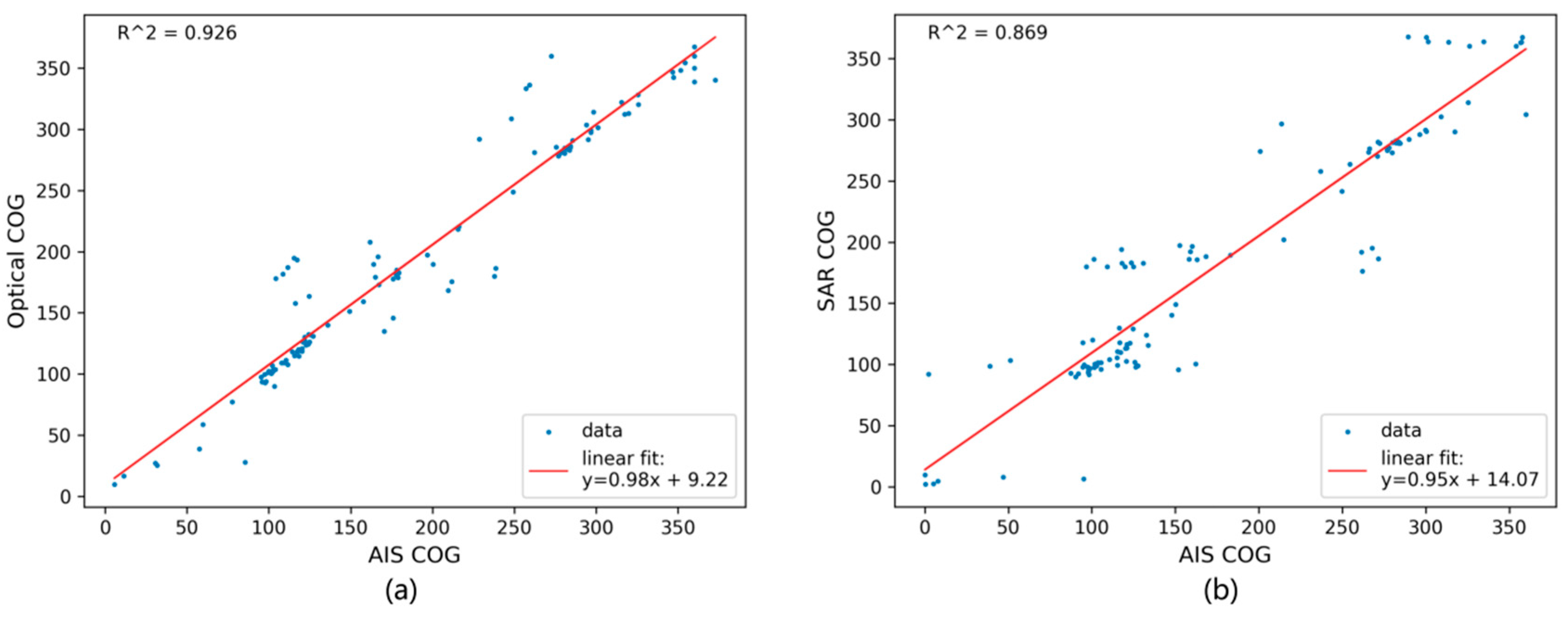
Figure 19a shows the relationship between the estimated course of each match pair in the optical case and the reported AIS course. The optical estimated course has good consistency with the AIS reported course. Figure 18b displays a similar chart for the SAR case. Similarly, the SAR estimated course has good consistency with the AIS-reported course, but is slightly inferior to the optical method. Moreover, the fitting effect of heading features is significantly better than that of length and width features in the optical case, while in the SAR case, the fitting effect of heading features is only slightly lower than that of length features. This indicates that the course feature plays a crucial role in data association, and its introduction helps improve the accuracy of ship target association.
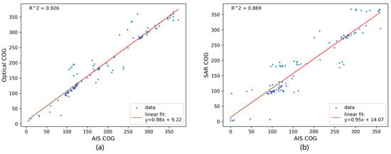
Figure 19.
Estimated (a) optical COG and (b) SAR COG against reported AIS.
In addition, we also conducted a comparative experiment of the association algorithm for different weight combinations, and the results are shown in Table 9. Different weight settings result in varying association rates and accuracies, with differences observed between the optical and SAR cases. In the optical case, the association rates increase from a minimum of 83.65% to a maximum of 96.03%, an increase of approximately 12.38%. The association accuracy fluctuates between 86.78% and 91.74%, with a difference of about 4.96%. In the SAR case, the association rates rise from a minimum of 64.89% to a maximum of 75.76%, an increase of approximately 10.87%. The association accuracy ranges from 85.71% to 91.33%, with a difference of about 5.62%. In summary, the position feature stands out as the paramount characteristic of point-to-point associations, meriting the greatest weight. The methodology presented in this paper exhibits a high level of consistency with regard to position features. Furthermore, course and length features likewise demonstrate good consistency, warranting a higher weight. Lastly, width features display instability and have a tendency to overestimate, particularly in the case of small vessels, necessitating a reduction in their weight. Combined with the association results and considering the association rate and association accuracy comprehensively, the weights for position, length, width, and course features in this method are set to [0.5, 0.2, 0.1, 0.2].
Table 9.
Association results for different weight combinations.
4.3. Effectiveness of Dark Ship Detection
This method detected 5 and 68 dark ships in the optical case and the SAR case, respectively. We estimated the length and width of the dark ships using target detection algorithms to calculate their aspect ratio. Then, we compared this ratio with the aspect ratios of successfully associated vessels, selecting the type of associated vessel with the smallest difference in aspect ratio as the predicted type of dark ship. The results show that in the optical case, the types of dark ships are cargo (3), dredging or underwater operation vessels (1), and others (1). In the SAR case, fishing boats predominate, with 48 vessels (70.6%), followed by a small number of cargo (5), tugs (4), yachts (2), container ships (1), and others (8). The significant difference in dark ship detection results between the optical and SAR cases is due to the distinct characteristics of vessels navigating the Bohai Strait during the day and night. During the day (in the optical case), the predominant types of vessels in the Bohai Strait include cargo ships, which account for 62.0% of the traffic, followed by oil tankers at 9.9%, and container ships at 8.3%. These figures are in line with the global trends where Chinese shipbuilding, known for its significant market share, has seen a rise in the production and export of these vessel types. Vessels shorter than 50 m accounted for only 7 (5.8%), and most vessels reported AIS information normally, with only a few missing AIS information (dark ships). However, at night (in the SAR case), fishing boats are the most numerous, accounting for 57.1%, followed by cargo (19.9%), yachts (3.6%), oil tankers (3.1%), and tugs (2.6%). There are 127 ships less than 50 m in length, accounting for 64.8%. These fishing ships often lack AIS equipment or fail to report AIS information, leading to a higher number of dark ships in SAR cases. Additionally, 50 (73.5%) of the dark ships in SAR cases are less than 50 m long. Due to the limitations of SAR resolution, even more small dark ships may go undetected. Based on the distribution differences of different types of dark ships during day and night, in practical monitoring strategies, daytime efforts can focus on large vessels such as cargo ships and oil tankers, taking the advantage of the high resolution of optical data to closely monitor their navigation paths and cargo transportation to prevent smuggling and illegal trade activities. At night, there should be increased supervision of fishing boats, combining the all-weather monitoring capabilities of SAR data to monitor whether fishing activities comply with regulations, preventing illegal fishing. At the same time, considering the characteristics of different types of vessels, detection algorithms and data association methods can be further optimized to improve monitoring efficiency and accuracy.
Furthermore, a failure to associate remote sensing images with AIS data can also occur when a ship has an AIS signal but is not detected in the remote sensing image. Such ships are not considered dark ships in this study, and we will briefly analyze the reasons for this situation. First, the coverage of AIS signals can extend beyond the radar and remote sensing images’ detection range, such as areas obscured by bridges or mountains. This means that even if the ship is physically obstructed, it may still not be detected by remote sensing images. Second, the accuracy of AIS data can be affected by the operational status of ship equipment and the interaction between satellites and receiving devices, potentially leading to geographical errors. If these errors exceed the matching threshold, the remote sensing image may fail to match the ship’s position recorded by AIS. Third, the imaging quality of remote sensing images can be compromised by complex sea conditions, leading to issues like blurriness and noise, which can prevent the identification of ships. To address these issues, improving the detection capabilities of ship targets and the precision of data correlation is essential. Additionally, enhancing data collection capabilities is a critical issue that needs to be addressed in future research.
In summary, this method can accomplish the task of detecting dark ships using multiple data sources such as optical remote sensing and SAR. Therefore, during marine monitoring, optical data can be prioritized during the day while switching to SAR data at night or in adverse weather conditions. The effective integration of optical and SAR data ensures precise monitoring of dark ships, aiding in the suppression of illegal activities.
5. Conclusions
This study addresses the core challenges of detecting dark ships by proposing an improved multi-feature satellite remote sensing and AIS data association method. By coordinating the use of optical and SAR data and improving data association algorithms, it effectively overcomes the shortcomings of traditional methods in terms of missing course features, mismatches in dense scenes, and monitoring timeliness. The “target detection-identity recognition” monitoring chain of this study efficiently fulfills the task of identifying dark ships, offering pivotal technical tools and methodological frameworks to bolster maritime safety. Multi-source data association technology can update the vessel dynamics database in real-time, providing high-precision trajectory support for collision warnings and search and rescue operations [47,48,49]. With the integration of satellite remote sensing and artificial intelligence technologies, it is anticipated that a comprehensive intelligent monitoring network will be established, encompassing all sea areas and times. This advancement is expected to propel maritime governance into a new era characterized by digitalization and precision.
The experimental results show that the proposed method has significant performance in dark ship detection accuracy, robustness, and multi-source collaboration ability. First, the YOLOv11-OBB model based on oriented bounding boxes successfully breaks through the directional representation limitations of traditional horizontal bounding boxes. The use of oriented bounding boxes allows for the precise extraction of ship shape and course features, providing a reliable foundation for subsequent data association. Second, by constructing a position-dimension-course multi-feature joint cost function and introducing an improved JVC global optimization algorithm, this study significantly enhances data association accuracy in dense shipping scenarios. Compared with the nearest neighbor (NN) method, the association rates of optical and SAR cases are increased by 11.90% and 9.47%, and the association accuracy of optical and SAR cases is increased by 1.06% and 5.62%, respectively. Upon comparison with the MSOA algorithm, it is observed that the association rate and association accuracy experience a significant enhancement, with increases of 4.76% and 3.04%, respectively. Especially in the SAR case, the detection of 68 dark ships validates the adaptability of the multi-feature joint method to complex scenarios. Finally, the collaborative monitoring framework of optical and SAR effectively compensates for the limitations of a single sensor. The combined application of the two provides dark ship detection with higher spatial and temporal coverage, which solves the problem of monitoring blind areas caused by cloud layer, light, and other factors in traditional methods.
Despite the significant progress made in this study, the following limitations remain: (1) The accuracy of small target detection is insufficient. Challenges remain in dealing with targets smaller than 10 pixels. (2) The computational complexity of multi-source data fusion and global optimization algorithms remains high, making it difficult to meet the emergency needs of maritime regulation. (3) Data coverage and generalization are inadequate. The current experimental dataset is limited in scope, primarily focusing on the Bohai Strait, which raises concerns about the adequacy of data coverage and generalization. It does not encompass remote seas or account for extreme weather conditions, such as typhoons, which are critical for comprehensive maritime data analysis.
In view of the above problems, future research can be carried out in the following directions: (1) Optimize the small target detection algorithm. Design an attention mechanism to enhance the network, focusing on indirect features such as ship wake. (2) Enhance real-time processing capabilities by exploring edge computing and model distillation technologies, enabling the deployment of algorithms onto devices for seamless end-to-end acceleration of the "detection-association-warning" chain. (3) Expand multi-source data fusion. Integrate data from multiple platforms, such as drones and buoy sensors, to build a three-dimensional monitoring network of land, sea, air, and sky. (4) Enhance the generalization of the algorithm. Establish a global multi-sea area ship data set, covering different climates, ocean currents, and ship types. Through transfer learning and domain adaptation technology, improve the model’s adaptability to the remote sea scene.
Author Contributions
Conceptualization, F.L. and C.Y.; data curation, F.L. and K.Y. (Kun Yu); formal analysis, F.L.; investigation, F.L. and C.Y.; methodology, F.L., K.Y. (Kun Yu) and C.Y.; resources, F.L., C.Y. and Y.T.; supervision, C.Y.; visualization, F.L.; writing—original draft, F.L.; writing—review and editing, C.Y., Y.T., G.Y., K.Y. (Kai Yin) and Y.L. All authors have read and agreed to the published version of the manuscript.
Funding
This research work was funded by the “Maritime Science and Technology Key Project Preliminary Basic Research Project” of the Maritime Safety Administration of the People’s Republic of China (E3DZ113401) and the “Research and Development of Key Technologies and Equipment for the New Generation of Marine Intelligent Transportation Management System” of the Hebei Transportation Investment Group Company Limited (E3E2113601).
Data Availability Statement
The original contributions presented in the study are included in the article, and further inquiries can be directed to the corresponding author.
Acknowledgments
The authors would like to thank the Northern Navigation Service Center, the Maritime Safety Administration, People’s Republic of China, for freely providing the AIS dataset.
Conflicts of Interest
The authors declare no conflicts of interest.
Abbreviations
The following abbreviations are used in this manuscript:
| AIS | Automatic Identification System. |
| SAR | Synthetic Aperture Radar. |
| ORS | Optical Remote Sensing. |
| OBB | Oriented Bounding Box. |
| CST | China Standard Time. |
| MMSI | Maritime Mobile Service Identity. |
| SOG | Speed Over Ground. |
| COG | Course Over Ground. |
References
- Prasad, M.S.; Verma, S.; Shichkina, Y.A. Dark Ship Detection: SAR Images. In Proceedings of the 2023 XXVI International Conference on Soft Computing and Measurements (SCM), St. Petersburg, Russia, 24–26 May 2023; pp. 341–344. [Google Scholar]
- Paolo, F.S.; Kroodsma, D.; Raynor, J.; Hochberg, T.; Davis, P.; Cleary, J.; Marsaglia, L.; Orofino, S.; Thomas, C.; Halpin, P. Satellite Mapping Reveals Extensive Industrial Activity at Sea. Nature 2024, 625, 85–91. [Google Scholar] [CrossRef] [PubMed]
- Huang, W.; Chen, S.; Wu, Y.; Li, R.; Li, T.; Huang, Y.; Cao, X.; Li, Z. DAShip: A Large-Scale Annotated Dataset for Ship Detection Using Distributed Acoustic Sensing Technique. IEEE J. Sel. Top. Appl. Earth Obs. Remote Sens. 2025, 18, 4093–4107. [Google Scholar] [CrossRef]
- Franceschetti, G.; Lanari, R.; Franceschetti, G.; Lanari, R. Synthetic Aperture Radar Processing; CRC Press: Boca Raton, FL, USA, 2018; ISBN 978-0-203-73748-4. [Google Scholar]
- Zhang, Z.; Zhang, L.; Wu, J.; Guo, W. Optical and Synthetic Aperture Radar Image Fusion for Ship Detection and Recognition: Current State, Challenges, and Future Prospects. IEEE Geosci. Remote Sens. Mag. 2024, 12, 132–168. [Google Scholar] [CrossRef]
- Zhao, Z.; Ji, K.; Xing, X.; Zou, H.; Zhou, S. Ship Surveillance by Integration of Space-Borne SAR and AIS—Review of Current Research. J. Navig. 2014, 67, 177–189. [Google Scholar] [CrossRef]
- Rodger, M.; Guida, R. Classification-Aided SAR and AIS Data Fusion for Space-Based Maritime Surveillance. Remote Sens. 2021, 13, 104. [Google Scholar] [CrossRef]
- Lang, H.; Wu, S.; Xu, Y. Ship Classification in SAR Images Improved by AIS Knowledge Transfer. IEEE Geosci. Remote Sens. Lett. 2018, 15, 439–443. [Google Scholar] [CrossRef]
- Rodger, M.; Guida, R. SAR and AIS Data Fusion for Dense Shipping Environments. In Proceedings of the IGARSS 2020—2020 IEEE International Geoscience and Remote Sensing Symposium, Waikoloa, HI, USA, 26 September–2 October 2020; pp. 2077–2080. [Google Scholar]
- Graziano, M.D.; Renga, A.; Moccia, A. Integration of Automatic Identification System (AIS) Data and Single-Channel Synthetic Aperture Radar (SAR) Images by SAR-Based Ship Velocity Estimation for Maritime Situational Awareness. Remote Sens. 2019, 11, 2196. [Google Scholar] [CrossRef]
- Caricchio, C.; Mendonça, L.F.; Lentini, C.A.D.; Lima, A.T.C.; Silva, D.O.; Meirelles e Góes, P.H. YOLOv8 Neural Network Application for Noncollaborative Vessel Detection Using Sentinel-1 SAR Data: A Case Study. IEEE Geosci. Remote Sens. Lett. 2025, 22, 4001005. [Google Scholar] [CrossRef]
- Chen, L.; Hu, Z.; Chen, J.; Sun, Y. SVIADF: Small Vessel Identification and Anomaly Detection Based on Wide-Area Remote Sensing Imagery and AIS Data Fusion. Remote Sens. 2025, 17, 868. [Google Scholar] [CrossRef]
- Galdelli, A.; Mancini, A.; Ferrà, C.; Tassetti, A.N. A Synergic Integration of AIS Data and SAR Imagery to Monitor Fisheries and Detect Suspicious Activities. Sensors 2021, 21, 2756. [Google Scholar] [CrossRef]
- Lee, Y.-K.; Jung, H.C.; Kim, K.; Jang, Y.; Ryu, J.-H.; Kim, S.-W. Assessment of Maritime Vessel Detection and Tracking Using Integrated SAR Imagery and AIS/V-Pass Data. Ocean Sci. J. 2024, 59, 27. [Google Scholar] [CrossRef]
- Liu, B.; Zhang, W.; Han, J.; Li, Y. Tracing Illegal Oil Discharges from Vessels Using SAR and AIS in Bohai Sea of China. Ocean Coast. Manag. 2021, 211, 105783. [Google Scholar] [CrossRef]
- Krizhevsky, A.; Sutskever, I.; Hinton, G.E. ImageNet Classification with Deep Convolutional Neural Networks. Commun. ACM 2017, 60, 84–90. [Google Scholar] [CrossRef]
- Handayani, D.O.D.; Sediono, W.; Shah, A. Anomaly Detection in Vessel Tracking Using Support Vector Machines (SVMs). In Proceedings of the 2013 International Conference on Advanced Computer Science Applications and Technologies, Kuching, Malaysia, 23–24 December 2013; pp. 213–217. [Google Scholar]
- Quinlan, J.R. C4.5: Programs for Machine Learning; Salzberg, S.L., Ed.; Morgan Kaufmann Publishers: Burlington, MA, USA, 1993; pp. 235–240. [Google Scholar] [CrossRef]
- Breiman, L. Random Forests. Mach. Learn. 2001, 45, 5–32. [Google Scholar] [CrossRef]
- Ren, S.; He, K.; Girshick, R.; Sun, J. Faster R-CNN: Towards Real-Time Object Detection with Region Proposal Networks. IEEE Trans. Pattern Anal. Mach. Intell. 2017, 39, 1137–1149. [Google Scholar] [CrossRef] [PubMed]
- Lin, T.-Y.; Dollár, P.; Girshick, R.; He, K.; Hariharan, B.; Belongie, S. Feature Pyramid Networks for Object Detection. In Proceedings of the 2017 IEEE Conference on Computer Vision and Pattern Recognition (CVPR), Honolulu, HI, USA, 21–26 July 2017; pp. 936–944. [Google Scholar]
- Redmon, J.; Divvala, S.; Girshick, R.; Farhadi, A. You Only Look Once: Unified, Real-Time Object Detection. In Proceedings of the 2016 IEEE Conference on Computer Vision and Pattern Recognition (CVPR), Las Vegas, NV, USA, 27–30 June 2016; pp. 779–788. [Google Scholar]
- Liu, W.; Anguelov, D.; Erhan, D.; Szegedy, C.; Reed, S.; Fu, C.-Y.; Berg, A.C. SSD: Single Shot MultiBox Detector. arXiv 2016, arXiv:1512.02325. [Google Scholar]
- Huang, Y.; Han, D.; Han, B.; Wu, Z. ADV-YOLO: Improved SAR Ship Detection Model Based on YOLOv8. J. Supercomput. 2024, 81, 34. [Google Scholar] [CrossRef]
- Wei, S.; Zeng, X.; Qu, Q.; Wang, M.; Su, H.; Shi, J. HRSID: A High-Resolution SAR Images Dataset for Ship Detection and Instance Segmentation. IEEE Access 2020, 8, 120234–120254. [Google Scholar] [CrossRef]
- Yasir, M.; Liu, S.; Pirasteh, S.; Xu, M.; Sheng, H.; Wan, J.; de Figueiredo, F.A.P.; Aguilar, F.J.; Li, J. YOLOShipTracker: Tracking Ships in SAR Images Using Lightweight YOLOv8. Int. J. Appl. Earth Obs. Geoinf. 2024, 134, 104137. [Google Scholar] [CrossRef]
- Sun, Z.; Leng, X.; Zhang, X.; Zhou, Z.; Xiong, B.; Ji, K.; Kuang, G. Arbitrary-Direction SAR Ship Detection Method for Multiscale Imbalance. IEEE Trans. Geosci. Remote Sens. 2025, 63, 5208921. [Google Scholar] [CrossRef]
- Zhao, Z.; Ji, K.F.; Xing, X.W.; Zou, H.X. Effective Association of SAR and AIS Data Using Non-Rigid Point Pattern Matching. IOP Conf. Ser. Earth Environ. Sci. 2014, 17, 012258. [Google Scholar] [CrossRef]
- Voinov, S.; Schwarz, E.; Krause, D.; Berg, M. Identification of SAR Detected Targets on Sea in Near Real Time Applications for Maritime Surveillance; University of Massachusetts: Amherst, MA, USA, 2017. [Google Scholar]
- Fabio, M.; Alfredo, A.; Herman, V.W.G.; Marlene, A.A.; Pietro, A.; Domenico, N.; Ziemba, L. Data Fusion for Wide-Area Maritime Surveillance; University of Pireaus: Pireas, Greece, 2013. [Google Scholar]
- Sandirasegaram, N.; Vachon, P.W. Validating Targets Detected by SAR Ship Detection Engines. Can. J. Remote Sens. 2017, 43, 451–454. [Google Scholar] [CrossRef]
- Pelich, R.; Chini, M.; Hostache, R.; Matgen, P.; Lopez-Martinez, C.; Nuevo, M.; Ries, P.; Eiden, G. Large-Scale Automatic Vessel Monitoring Based on Dual-Polarization Sentinel-1 and AIS Data. Remote Sens. 2019, 11, 1078. [Google Scholar] [CrossRef]
- Zhao, Z.; Ji, K.; Xing, X.; Zou, H. Research on High-Accuracy Data Association of Space-Borne SAR and AIS. In Proceedings of the 2013 Chinese Intelligent Automation Conference; Sun, Z., Deng, Z., Eds.; Springer: Berlin/Heidelberg, Germany, 2013; pp. 359–367. [Google Scholar]
- Liu, Z.; Xu, J.; Li, J.; Plaza, A.; Zhang, S.; Wang, L. Moving Ship Optimal Association for Maritime Surveillance: Fusing AIS and Sentinel-2 Data. IEEE Trans. Geosci. Remote Sens. 2022, 60, 5635218. [Google Scholar] [CrossRef]
- Khanam, R.; Hussain, M. YOLOv11: An Overview of the Key Architectural Enhancements. arXiv 2024, arXiv:2410.17725. [Google Scholar]
- Crouse, D.F. On Implementing 2D Rectangular Assignment Algorithms. IEEE Trans. Aerosp. Electron. Syst. 2016, 52, 1679–1696. [Google Scholar] [CrossRef]
- cgvict Cgvict/roLabelImg. Available online: https://github.com/cgvict/roLabelImg (accessed on 9 April 2025).
- Li, J.; Qu, C.; Shao, J. Ship Detection in SAR Images Based on an Improved Faster R-CNN. In Proceedings of the 2017 SAR in Big Data Era: Models, Methods and Applications (BIGSARDATA), Beijing, China, 13–14 November 2017; pp. 1–6. [Google Scholar]
- Lei, S.; Lu, D.; Qiu, X.; Ding, C. SRSDD-v1.0: A High-Resolution SAR Rotation Ship Detection Dataset. Remote Sens. 2021, 13, 5104. [Google Scholar] [CrossRef]
- Ultralytics OBB. Available online: https://docs.ultralytics.com/zh/tasks/obb (accessed on 21 April 2025).
- Zhang, C.; Zhang, X.; Gao, G.; Lang, H.; Liu, G.; Cao, C.; Song, Y.; Guan, Y.; Dai, Y. Development and Application of Ship Detection and Classification Datasets: A Review. IEEE Geosci. Remote Sens. Mag. 2024, 12, 12–45. [Google Scholar] [CrossRef]
- Ding, J.; Xue, N.; Long, Y.; Xia, G.-S.; Lu, Q. Learning RoI Transformer for Oriented Object Detection in Aerial Images. In Proceedings of the 2019 IEEE/CVF Conference on Computer Vision and Pattern Recognition (CVPR), Long Beach, CA, USA, 15–20 June 2019; pp. 2844–2853. [Google Scholar]
- Han, J.; Ding, J.; Li, J.; Xia, G.-S. Align Deep Features for Oriented Object Detection. IEEE Trans. Geosci. Remote Sens. 2022, 60, 5602511. [Google Scholar] [CrossRef]
- China Platform of Earth Observation System (CPEOS). Available online: https://www.cpeos.org.cn/home/#/rsSatelliteIntro (accessed on 3 April 2025).
- Brusch, S.; Lehner, S.; Fritz, T.; Soccorsi, M.; Soloviev, A.; van Schie, B. Ship Surveillance With TerraSAR-X. IEEE Trans. Geosci. Remote Sens. 2011, 49, 1092–1103. [Google Scholar] [CrossRef]
- Greidanus, H.; Alvarez, M.; Santamaria, C.; Thoorens, F.-X.; Kourti, N.; Argentieri, P. The SUMO Ship Detector Algorithm for Satellite Radar Images. Remote Sens. 2017, 9, 246. [Google Scholar] [CrossRef]
- Zhao, C.; Bao, M.; Liang, J.; Liang, M.; Liu, R.W.; Pang, G. Multi-Sensor Fusion-Driven Surface Vessel Identification and Tracking Using Unmanned Aerial Vehicles for Maritime Surveillance. IEEE Trans. Consum. Electron. 2025; early access. [Google Scholar] [CrossRef]
- Huang, Y.; Liu, W.; Lin, Y.; Kang, J.; Zhu, F.; Wang, F.-Y. FLCSDet: Federated Learning-Driven Cross-Spatial Vessel Detection for Maritime Surveillance with Privacy Preservation. IEEE Trans. Intell. Transp. Syst. 2025, 26, 1177–1192. [Google Scholar] [CrossRef]
- Zhang, B.; Liu, J.; Liu, R.W.; Huang, Y. Deep-Learning-Empowered Visual Ship Detection and Tracking: Literature Review and Future Direction. Eng. Appl. Artif. Intell. 2025, 141, 109754. [Google Scholar] [CrossRef]


Disclaimer/Publisher’s Note: The statements, opinions and data contained in all publications are solely those of the individual author(s) and contributor(s) and not of MDPI and/or the editor(s). MDPI and/or the editor(s) disclaim responsibility for any injury to people or property resulting from any ideas, methods, instructions or products referred to in the content. |
© 2025 by the authors. Licensee MDPI, Basel, Switzerland. This article is an open access article distributed under the terms and conditions of the Creative Commons Attribution (CC BY) license (https://creativecommons.org/licenses/by/4.0/).