Abstract
Tropical forests harbor a significant portion of global biodiversity but are increasingly degraded by human activity. Assessing restoration efforts requires the systematic monitoring of tropical ecosystem status and recovery. Satellite-borne synthetic aperture radar (SAR) supports monitoring changes in vegetation structure and is of particular utility in tropical regions where clouds obscure optical satellite observations. To characterize tropical forest recovery in the Lowland Chocó Biodiversity Hotspot of Ecuador, we apply over a decade of dual-polarized (HH + HV) L-band SAR datasets from the Japanese Space Agency’s (JAXA) PALSAR and PALSAR-2 sensors. We assess the complementarity of the dual-polarized imagery with less frequently available fully-polarimetric imagery, particularly in the context of their respective temporal and informational trade-offs. We examine the radar image texture associated with the dual-pol radar vegetation index (DpRVI) to assess the associated determination of forest and nonforest areas in a topographically complex region, and we examine the equivalent performance of texture measures derived from the Freeman–Durden polarimetric radar decomposition classification scheme applied to the fully polarimetric data. The results demonstrate that employing a dual-polarimetric decomposition classification scheme and subsequently deriving the associated gray-level co-occurrence matrix mean from the DpRVI substantially improved the classification accuracy (from 88.2% to 97.2%). Through this workflow, we develop a new metric, the Radar Forest Regeneration Index (RFRI), and apply it to describe a chronosequence of a tropical forest recovering from naturally regenerating pasture and cacao plots. Our findings from the Lowland Chocó region are particularly relevant to the upcoming NASA-ISRO NISAR mission, which will enable the comprehensive characterization of vegetation structural parameters and significantly enhance the monitoring of biodiversity conservation efforts in tropical forest ecosystems.
1. Introduction
Tropical forests provide critical ecosystem services and comprise a significant portion of global biodiversity but face significant threats from anthropogenic degradation and associated land-use changes. The complex nature of these densely vegetated ecosystems makes fully understanding their structure and function challenging [1,2]. Human activities that cause fragmentation and deforestation further exacerbate these challenges and directly affect species distribution and conservation efforts [3,4]. Efforts to restore biodiversity through reforestation have gained attention but require improvements to the characterization of tropical ecosystems in terms of their structure, function, and spatiotemporal variability [5,6]. Recognizing the urgency of this task, there is a need for advancing methods for detecting land cover changes, accurately reconstructing disturbance history, and understanding the dynamics of tropical ecosystem regeneration.
Advancements in remote sensing techniques have significantly enhanced our ability to monitor changes in the tropical ecosystem habitat structure from degradation, fragmentation, and forest regeneration resulting from human activity [7]. However, the effectiveness of long-standing spaceborne remote sensing programs such as Landsat in monitoring land cover changes in biodiversity hotspots has historically been hindered by cloud cover over tropical forest ecosystems. Additionally, while global deforestation products perform well over large areas, they often lack the detailed granularity needed to capture the early stages of land cover degradation and habitat changes occurring beneath the forest canopy, such as selective logging and road development [8,9].
Active microwave observations obtained from synthetic aperture radar (SAR) offer a means to monitor changes in land surface and vegetation structure, including processes related to tropical forest degradation and regeneration [10,11]. SAR systems can detect variations in the structural and moisture characteristics of terrestrial ecosystems, as SAR backscatter is dependent on both sensor properties (such as wavelength and polarization) and surface characteristics (e.g., vegetation structure and water content) [12,13]. Importantly, SAR sensors are not hindered by cloud cover or nighttime conditions, enabling the effective monitoring of tropical ecosystems at moderate-to-high spatial resolutions (~10 to 20 m) and temporal revisits (typically on a weekly to monthly basis). Furthermore, SAR sensors operating at longer wavelengths, specifically L-band SAR, transmit signals that penetrate into vegetation canopies to a greater degree than C-band SAR, thereby providing greater sensitivity to characteristics and changes in forest structure.
SAR systems can acquire data in multiple polarizations, offering more detailed structural information about surface targets. This makes multi-channel L-band imagery particularly well-suited for forest disturbance applications [14,15,16]. Moreover, indices derived from polarimetric SAR imagery, such as the radar vegetation index (RVI), can mitigate topographic effects, exhibit sensitivity to forested areas, and enable the monitoring of forest regrowth when time series data are accessible [17]. Furthermore, the decomposition of fully polarimetric (full-pol) imagery offers an enhanced method for classifying radar scenes by separating SAR data into fundamental scattering components from surface targets [18]. More recently, the decomposition of dual-polarization (dual-pol) data has facilitated the derivation of the dual-pol radar vegetation index (DpRVI) [19]. The DpRVI is notably distinct from previous dual-polarization radar vegetation indices derived from only intensity information. Leveraging dual-pol decompositions that include intensity and phase information is becoming increasingly advantageous with the expanding archive of Sentinel-1 and PALSAR-2 imagery, and as well as with the forthcoming NISAR mission, which will provide high-resolution, open-access L-band HH and HV imagery for the global land area.
Furthermore, the utilization of radar image texture derivation has demonstrated its capability in classifying a range of tropical land cover types and supporting broader landscape characterization efforts [20,21,22]. This includes applications in higher-resolution L-band SAR data, where texture metrics—which quantify spatial variability in backscatter—can help mitigate speckle noise and enhance the detection of landscape heterogeneity relevant to ecological processes such as forest degradation and regeneration [23]. Unlike first-order statistics, second-order measures derived from the gray-level co-occurrence matrix (GLCM) capture the interrelationship between pairs of pixels [24]. This proves valuable in landscape-scale applications, such as detecting patches of forest degradation and tracking the progression of deforestation, which often exhibit spatial patterns influenced by local topography and land-use history [25].
Research using full-pol L-band imagery to analyze texture has historically encountered limitations in temporal coverage, often constrained to data from a single scene. This constraint restricts the time series analysis of land cover changes, such as with forest degradation or regeneration assessments. The utilization of texture in time series analyses is more common with C-band systems, e.g., Sentinel-1 [26]. However, such analyses with C-band SAR are generally more effective for agricultural applications rather than for monitoring tropical forests, as high-biomass systems such as dense canopies can lead to signal saturation and reduce the utility of C-band data in these contexts [27,28]. Several studies have incorporated a combination of measures derived from both L-band and C-band sensors into classification schemes [26,29,30]. However, these approaches can be methodologically complex and difficult to reproduce due to temporal discrepancies between observations from different systems. Despite the increasing availability of L-band SAR data, few studies have leveraged the time series of textural measures to monitor forest regeneration—an important methodological and ecological gap this study seeks to fill. Innovative methodologies that combine time series L-band dual-pol decompositions with texture image derivations may offer an approach to better capture crucial aspects of forest degradation and regeneration processes. Furthermore, upcoming SAR missions like NISAR are expected to bring significant advancements in forest monitoring capabilities [31]. NISAR will feature dual L-band and S-band acquisitions with frequent revisit periods of approximately 12 days, offering potential for significant breakthroughs in areas such as biomass estimations and forest degradation mapping [32].
The overall objective of this study is to monitor tropical forest disturbance and recovery using an extended time series of spaceborne L-band SAR imagery (2007–2019), deriving measures from dual-pol data that achieve classification accuracy comparable to full-pol observations. We conduct this analysis by generating measures of texture from the decomposition of dual-pol imagery. These measures are then applied to time series investigations of forest regeneration across retrospective and contemporary PALSAR and PALSAR-2 archives. We first develop a reference forest/nonforest product using GLCM texture measures derived from the Freeman–Durden decomposition of a full-pol 2015 PALSAR-2 scene. We then assess a comparable classification using GLCM texture measures derived from the DpRVI based on the complex matrix. Lastly, we normalize the DpRVI GLCM mean derivation to develop a new radar metric, the Radar Forest Regeneration Index (RFRI), and employ the RFRI to describe a chronosequence of regenerating tropical forest plots in the Lowland Chocó Biodiversity Hotspot of Ecuador with long-term PALSAR and PALSAR-2 observations.
2. Materials and Methods
2.1. Study Area and Datasets
The region of study is the lowland rainforest of northwest Ecuador within the Chocó Biodiversity Hotspot (Figure 1). The Chocó ecoregion is among the highest priorities for conservation worldwide [33]. Less than two percent of the Chocó primary forest remains as a result of the recent expansion of the agricultural frontier driven by legal and illegal logging [34]. The most significant degradation and habitat loss occurred over the last 40 years due to deforestation, primarily driven by the expansion of the agroindustry and oil palm plantations [33,35,36]. Reconstructing the land-use change history of this region remains challenging as the Chocó is obscured by cloud cover nearly 90% of the time, among the highest amount globally [37]. The limited availability of satellite-based, cloud-free optical imagery for the Lowland Chocó has hindered conservation efforts, including the monitoring of protected areas and the assessment of forest regeneration.
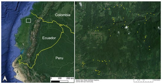
Figure 1.
Study region location (white box) in the Lowland Chocó rainforest of Ecuador (left) and distribution of 64 validation plots (yellow dots) that include the following classes: active pasture, active cacao, regenerating pasture, regenerating cacao, and old-growth forest (right).
We investigated a chronosequence of forest recovery captured along 64 in situ study plots located within the Canandé (Fundación Jocotoco) and Tesoro Escondido Forest reserves, as well as surrounding habitats within a 182 km2 region of the Lowland Chocó. This region also includes adjacent conservation efforts in the Itapoa Reserve. The validation plots in this study were established as part of the German Research Foundation (DFG) funded German–Ecuadorian collaborative Research Unit “Reassembly of species interaction networks”, REASSEMBLY (FOR 5207) [38]. These plots included 8 plots in active pastures, 7 plots in active cacao plantations, 15 regenerating forest plots (hereafter noted as regenerating plots) after previous use as pastures, 17 regenerating plots after previous use as cacao plantations, and 17 plots in an old-growth forest. The alpha-numeric identifier, landcover class, and regeneration year for each of the 64 plots are provided in Appendix A. Each plot measured approximately 50 m × 50 m and was surrounded by a similar land cover type and recovery age. The time of regeneration in secondary forest plots (i.e., regenerating from cacao or pasture) ranged from 0 to 35 years, where 0 years corresponds to the point at which a site was placed under conservation protection and agricultural activities were abandoned, allowing natural forest regeneration to begin. Agricultural abandonment across the 64 study plots occurred between 1985 and 2019, forming the basis for the regeneration chronosequence analyzed here (Figure 2). Further details on plot history and characteristics are provided in Escobar et al. (2025) [38]. Forest ages and land-use history were determined through a combination of local interviews and information gathered from land acquisitions through Fundación Jocotoco. Old-growth forest (hereafter, forest) plots represented a primary reference state, but like most tropical forests, were likely impacted by anthropogenic activities at some point in the past [39]. The minimum and maximum distances between plots of the same type were 1023 m and 9847 m (cacao), 1547 m and 9384 m (pasture), 231 and 12,085 m (regenerating forest, previously cacao), 288 m and 10,875 m (regenerating forest, previously pasture), and 361 m and 12,624 m (forest) across an elevation range of 159–615 m.

Figure 2.
Natural recovery chronosequence of active land cover classes considered in this study from pasture (top) and cacao plantation (bottom) to old-growth forest (right). The number of years indicates the approximate amount of time each plot has been naturally regenerating since achieving conservation status. Image source: https://www.reassembly.de/ (accessed on 2 February 2025).
We utilized SAR data from PALSAR and PALSAR-2 in our time series investigation of Lowland Chocó forest regeneration between 2007 and 2019. PALSAR acquired imagery of the study location from 2007 to 2010 and PALSAR-2 acquired imagery of the study location from 2015 to 2019. Both sensors operate at L-band, 22.9 cm wavelength, and acquire data in fully-polarimetric (full-pol) and dual-polarimetric (dual-pol) HH and HV modes. In this study, the term “full-pol” refers to linear quad-polarimetric data. A total of fourteen SAR scenes, including one full-pol image, were utilized in this study (Table 1). Imagery was acquired from both ascending and descending orbits with staggered monthly and annual revisit times, depending on mission and acquisition mode. All imagery was downloaded in Level 1.1 (L1.1) single look complex (SLC) format. In our workflow, the PALSAR-2 full-pol data were utilized to develop a ‘benchmark’ forest/nonforest map for the year 2015. We considered the 2015 PALSAR-2 scene as the reference observation in our imagery stack because it was both the highest resolution (2.9 × 2.8 m) and the only full-pol image. We also developed a texture based dual-pol classification approach using this same 2015 scene, and we demonstrated that this dual-pol classification resulted in a comparable classification accuracy to the full-pol approach. Subsequently, we derived texture measures from time series dual-pol PALSAR and PALSAR-2 imagery, enabling the analysis of a multi-decade chronosequence of tropical forest regeneration in the Lowland Chocó of Ecuador.

Table 1.
PALSAR and PALSAR-2 acquisitions spanning 12 years over the Lowland Chocó study site. The incidence angle is reported at the center of the test area center.
2.2. Polarimetric SAR Pre-Processing and Derivation of Vegetation Indices
Figure 3 diagrams the processing workflow applied to complex full-pol and dual-pol imagery for polarimetric decomposition and subsequent analysis. The pre-processing of the full-pol 2015 PALSAR-2 single look complex data was accomplished using the Sentinel-1 Toolbox within the Sentinel Application Platform (SNAP; https://step.esa.int (accessed on 12 December 2024)). The pre-processing steps included the radiometric calibration of real and imaginary (i, q) bands to produce complex SAR data, application of the Polarimetric Refined Lee speckle filter with a 5 × 5 window, and computation of the coherency matrix (T3) from the polarimetric covariance data [40,41,42]. The Freeman–Durden decomposition was employed using a 5 × 5 window size to produce fractional estimates of the double-bounce, volume, and surface scattering mechanism contribution to total backscatter [18]. We chose the Freeman–Durden decomposition (FD) due to its established effectiveness in classifying land cover, particularly in forested areas [43,44]. We applied terrain correction to account for the topographic correction of pixel locations [45]. The terrain correction operator in SNAP also generated a local incidence angle map, which was later utilized in the workflow to assess the predominant scattering mechanism in regions of high relief, beyond the forest regeneration study plots [46,47]. The resulting decomposition product was resampled to a 12.5 × 12.5 m resolution in local UTM coordinates to harmonize the spatial scale with the ALOS PALSAR-derived data used in the multi-temporal analysis, resulting in georeferenced scattering component layers (double-bounce, volume, and surface) suitable for integration into subsequent classification and time series modeling.
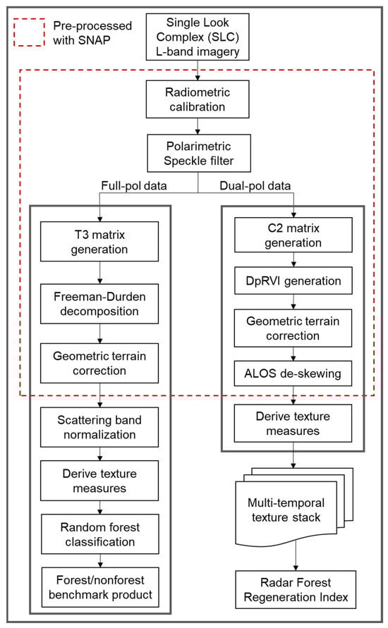
Figure 3.
Polarimetric SAR processing workflow for forest/nonforest mapping and regeneration analysis. The full-pol data route is the forest/nonforest classification workflow to develop the benchmark forest product from Freeman–Durden decomposition of full-polarization L-band imagery. The dual-pol data route is the time series workflow to develop the Radar Forest Regeneration Index (RFRI) product from polarimetric decomposition of dual-polarization L-band imagery.
The pre-processing of the dual-pol multi-temporal stack was similarly accomplished using SNAP, as shown in Figure 3. Our particular interest was in computing the dual-polarization radar vegetation index (DpRVI) for each scene within the 2007–2019 time series. The DpRVI processing chain included the radiometric calibration of the complex HH and HV channels, application of the Polarimetric Refined Lee speckle filter (5 × 5 window), and construction of the covariance matrix—all prerequisite steps for calculating the DpRVI using dual-polarization SAR data. The DpRVI is computed from the covariance matrix, following the formulation in Mandal et al. (2020) [19], and serves as a proxy for the scattering complexity of a given resolution cell. The degree of polarization, , is calculated as follows:
where Tr denotes the trace operator (i.e., the sum of the diagonal elements of the matrix), and represents the determinant of a matrix [48]. The DpRVI is then defined as follows:
where is a randomness weighting factor described in Mandal et al. (2020) [19]. All products were then terrain corrected to a 12.5 m resolution in local UTM projection. In the case of PALSAR data, an additional ALOS de-skewing step was included before terrain correction. Since ALOS L1.1 data are distributed in squinted geometry; the de-skewing operator transfers the data into a zero Doppler-like geometry prior to applying standard SAR processing. The de-skewing of ALOS-2 products is unnecessary as they are provided in a zero Doppler geometry.
Higher DpRVI values are typically associated with increased volumetric and depolarized scattering, common in vegetated or structurally complex tropical environments. Because the DpRVI is a recently developed approach incorporating both phase and intensity information to identify vegetation scattering, we compared the DpRVI to the dual-pol radar forest degradation index (RFDI)-based backscatter. Utilizing the same dual-pol multi-temporal dataset, pre-processing was conducted in SNAP, following standard procedures: radiometric calibration, speckle filtering using the Refined Lee filter (5 × 5 window), and terrain correction to ground range projection, yielding and backscatter layers. The data were resampled to a 12.5 m resolution in local UTM coordinates. We computed the radar forest degradation index (RFDI) utilizing and in the following formula [49]:
To extend the comparison between the full-pol Freeman–Durden decomposition and the dual-pol time series analysis, we derived the radar vegetation index (RVI) from the full-pol 2015 PALSAR-2 reference scene for a comparative analysis. Pre-processing followed the same approach as the dual-pol dataset but was applied specifically to the 2015 full-pol image, producing , , , and backscatter layers. The L-band radar vegetation index (RVI) was computed using the following standard equation:
where represents the radiometrically and geometrically corrected SAR backscattering coefficient in linear units for each polarization.
2.3. Scattering Contribution Normalization
The radar indices, including the DpRVI, RVI, and RFDI, effectively reduce the influence of topography on image classification across the PALSAR AND PALSAR-2 scenes. However, topographic artifacts persisted in the Freeman–Durden decomposition product (Figure 4). To mitigate these effects, we performed a component-wise normalization process. First, each scattering mechanism band—double-bounce (DB), volume (VS), and surface (SS)—was converted from decibels (dB) to linear-scale backscatter power. These values were then normalized by their total sum to compute the relative contribution of each scattering component within each pixel, as shown in Equations (5)–(8):
where pwr denotes the linear-scale scattering power (converted from dB), is the total backscatter power across components, and PN represents the proportion of each scattering mechanism normalized within each pixel. This formulation follows the convention of Freeman–Durden-type decompositions and aligns with the approach used by Sugimoto et al. (2022), who performed a tropical forest classification based on normalized scattering power contributions [50]. This implementation offers an effective method for incorporating additional imagery in time series analyses. Normalizing to total power mitigates the impact of incidence angle variations, which is particularly beneficial in regions with a complex topography. This enables the integration of time series imagery acquired from different orbital directions, compensating for cases where there are insufficient co-orbital scenes for a robust forest regeneration analysis.

Figure 4.
Comparison of Freeman–Durden polarimetric decomposition outputs using three scaling representations: decibel units (left), linear-scale backscatter power (middle), and power normalized to total backscatter power (right). RGB false-color composites were generated by assigning double-bounce, volume, and surface scattering powers to the red, green, and blue channels, respectively. Areas dominated by volume scattering (green) typically correspond to mature, closed-canopy forest stands in the northern portion of the study region, where recent anthropogenic disturbance is minimal. In contrast, areas of recent deforestation exhibit elevated surface scattering, while plantation and pasture areas in flatter southern regions show characteristic double-bounce and surface-dominated returns. Normalization (right) reduces terrain-related artifacts, highlighting scattering contributions independent of topographic modulation.
2.4. Generating Texture Measures
We computed measures of texture from DBPN, VSPN, SSPN, , , and DpRVI to assess their potential to improve forest/nonforest classifications. We explored first-order texture statistics, including the coefficient of variation (cv), along with standard Haralick texture measures extracted from the gray-level co-occurrence matrix (GLCM) [24]. These measures of texture are defined in Appendix A.
Next, we conducted a validation exercise to assess how effectively our derived radar texture measures could distinguish between various land cover types in the Lowland Chocó study area. Each texture measure was evaluated based on its capacity to differentiate between forest and nonforest land cover classes. We conducted an analysis of variance (ANOVA) to determine the relative effectiveness of texture measures in terms of separating land cover classes. Ultimately, the GLCM mean (GLCMm) showed the most significant improvement in distinguishing forest from nonforest sites and thus was selected as the texture measure for use in the subsequent classification exercises. A further discussion on these findings is provided in Section 3.1.
2.5. Developing Classification Maps from Full-Pol and Dual-Pol Imagery to Enhance Forest/Nonforest Detection
We developed a forest/nonforest reference product through a supervised random forest classification, utilizing textural features derived from the Freeman–Durden (FD) decomposition of a full-pol PALSAR-2 image obtained in 2015 as input variables, with training data from established ecological study plots [38]. We termed this route the full-pol Freeman–Durden (FpFD) approach. The examination of regions with a steep terrain show the contribution of double-bounce scatter to be negligible within the land classes in our study region, consistent with topographic effects reported in other studies [51,52]. We found volume scatter to be the dominant scattering mechanism from forests, whereas double-bounce scatter contributed only a small fraction per pixel to the overall backscatter, and the surface scatter was more evenly split with the volume scatter in pasture regions. We observed that in the Lowland Chocó region, the double-bounce scatter was predominantly associated with oil palm plantations and urban centers, which lie in regions of minimal relief to the south beyond our forest conservation region of study (Figure 4). These findings were corroborated through extensive ground-based field observations conducted by the authors in 2015, as well as in preceding and subsequent years, along with visual confirmation using available cloud-free optical satellite imagery from both multispectral and high-resolution commercial sources (see Escobar et al., 2025 for additional methodological detail) [38]. Table 2 shows the mean and standard deviation of double-bounce normalized (DBPN), volume scatter normalized (VSPN), and surface scatter normalized (SSPN) results for each representative land cover type in the study region. This lent support for our full-pol classification approach, which uses only VSPN and SSPN as input variables to distinguish between forest and nonforest regions.
Table 2.
L-band scattering contribution normalized to total power from full-polarimetric decomposition of 2015 PALSAR-2 acquisition for study classes within the Lowland Chocó. Pasture, cacao, and forest are fixed classes through the study’s temporal domain. Pasture regeneration and cacao regeneration classes are dynamic study plots along a regrowth chronosequence from 0 to 35 years after conservation.
In the random forest classifier, the forest class was trained exclusively on forested sites, while the nonforest class included both active pasture and cacao study plots. The nonforest training class included both the active pasture and cacao study plots. In this temporally fixed reference classification, we did not include the regenerating pasture and regenerating cacao study plots. The configuration of the classifier included initializing the model with 500 trees, splitting ground-validation datasets into 70% training and 30% testing groups, and balanced subsampling class weighting. The latter accounted for the different populations within each class and automatically adjusted class weights in a way that was inversely proportional to class frequencies based on the bootstrap sample for every tree grown.
Using the same classifier setup, we derived comparable forest/nonforest classifications using the RVI and DpRVI products as the input variables, respectively. Table 3 summarizes the classification approaches considered in this study. In the approach with FpFD, VSPN and SSPN were used as input variables, while the approaches beginning with the RVI and DpRVI utilized each index exclusively. Subsequently, we replaced the parent radar products (FpFD, RVI, and DpRVI) with their derived GLCMm texture measure as input variables for classification (FpFD replaced with VSPN GLCMm and SSPN GLCMm; RVI replaced with RVI GLCMm; DpRVI replaced with DpRVI GLCMm). We compared these results with classification approaches without texture features as input variables, i.e., FpFD, RVI, and DpRVI only. The classification accuracy and forest/nonforest mapping results are detailed in Section 3.2.
Table 3.
Summary of the forest/nonforest classification approaches and input variables considered in this study. Texture in the classification approach is the computed gray-level co-occurrence matrix mean (GLCMm) from the corresponding initial L-band product. VSPN and SSPN classification input variables are the power normalized volume scatter and surface scatter components derived from the fully-polarimetric Freeman–Durden (FpFD) decomposition. Confusion matrix results from each classification approach are provided in Appendix B.
2.6. Texture Normalization for Temporal Analysis
We leveraged the time series dual-pol imagery to expand our analysis and examine the regenerating pasture and regenerating cacao classes. This involved analyzing changes in image texture over time. We normalized the DpRVI GLCM mean images obtained from the PALSAR AND PALSAR-2 observations between 2007 and 2019 (Table 1) to create a new metric termed the Radar Forest Regeneration Index (RFRI).
Texture measures are typically dimensionless and are commonly used to gain insight into different land cover types within a single scene. However, we observed GLCMm values ranging from 0 to 125 across all images in the time series within our study region. The lowest GLCMm values, 0, were associated with open water, while the highest values, 125, were linked to old-growth forest regions, both of which remained constant throughout the study period. Leveraging these textural endpoints, we developed the RFRI measure for the temporal forest regeneration analysis from complex dual-pol data. The RFRI is calculated through the max–min normalization of the GLCMm derived from the DpRVI, scaled from 0 to 1, as follows:
where the GLCMm is the GLCM mean value at each pixel, the GLCMmin is the minimum GLCM mean value within the scene, and the GLCMmax is the maximum GLCM mean value within each scene. The max–min normalization of the unitless GLCMm texture measure maintained the statistical distribution of pixels within each scene, enabling meaningful comparisons between scenes over time.
We employed the time series imagery to create a comprehensive classification map that includes a transitioning forest class, in addition to the forest and nonforest classes. Using the random forest classifier with the RFRI stack as input variables, we incorporated training data for the transitioning forest class, encompassing both regenerating pasture and regenerating cacao study plots. However, to ensure a conservative approach, we excluded regenerating plot data for periods of less than 5 years and greater than 30 years of regeneration. This was based on our results (Section 3.3), indicating that RFRI values at these ends of the chronosequence spectrum are more representative of the nonforest and forest class textures, respectively. This grouped class was labeled ‘transitioning’ to account for both forest regeneration and potential forest degradation that may have occurred across the Lowland Chocó study region during the observed temporal period. The classification results are detailed in Section 3.3.
To evaluate the utility of the RFRI in the forest regeneration analysis, we explored changes in the RFRI over the time series for each study class. We assessed its effectiveness compared to L-band measures , , the cross-polarization ratio , and the radar forest degradation index (RFDI) for determining forest regeneration statistics. In this temporal analysis, each plot was analyzed based on ‘Regeneration Years’, defined as the duration between the year a site achieved conservation protection status, allowing natural forest regeneration to begin, and the date of satellite image observation. These results are detailed in Section 3.3.
3. Results
Below, we present results from three major components of our analysis, each of which is detailed in its respective subsection: (1) the evaluation and selection of SAR-based texture measures to improve class separability between tropical forest and nonforest areas, (2) a comparison of forest/nonforest classification accuracy using full- and dual-pol SAR data, including improvements gained through texture substitution, and (3) a temporal assessment of forest regeneration using a long-term SAR time series to classify transitional forest cover areas. These analyses are validated using independent field plot survey data.
3.1. Forest/Nonforest Texture Analysis
We conducted an analysis of variance (ANOVA) to determine the extent to which L-band radar backscatter, associated indices, and texture statistics can differentiate between the forest and nonforest study plots in the 2015 full-pol PALSAR-2 reference scene. The results for each radar measure and its derived texture measure are provided in Table 4. Among nearly all radar measures, the GLCM mean (GLCMm) was the texture measure that most effectively distinguished between the forest and nonforest classes, as indicated by its significantly higher F-score (e.g., DpRVI: F1,446 = 756; p < 0.0005). The GLCM Variance (GLCMvar) also effectively distinguished between classes (DpRVI: F1,446 = 634; p < 0.0005), although GLCMvar F-scores across all measures were not as high compared with the GLCMm. The sole exception was in the results for backscatter, where the first-order coefficient of variation achieved the highest F-score (F1,446 = 82; p < 0.0005). However, all statistically significant results of the GLCMm and GLCMvar derived from other L-band SAR measures exhibited substantially higher F-scores (Table 4). This suggests that relying exclusively on texture derivations from backscatter is insufficient for effectively distinguishing between the forest and nonforest classes.
Table 4.
ANOVA F-scores indicating the differentiation between forest and nonforest classes based on texture measures derived from L-band and backscatter, surface scatter normalized (SSPN), volume scatter normalized (VSPN), radar vegetation index (RVI) and dual-pol radar vegetation index (DpRVI). The significance threshold for the F-critical value is 5.
The remaining texture measures exhibited a diminished capability to distinguish between the forest and nonforest classes compared to their parent radar measures (Table 4). While contrast and dissimilarity displayed F-scores more than 50 points higher across certain measures (e.g., VSPN and DpRVI), the energy, entropy, homogeneity, and second moment showed decreased effectiveness (lower F-values) in separating classes compared to their respective parent measures alone.
Figure 5 provides a visual indication of the ability of texture measures to distinguish between the forest and nonforest study plots. We present the results of selected texture measures derived from the DpRVI, which serve as the basis for the temporal regeneration analysis in our methodology. Both the boxplots and kernel density estimates in Figure 5 illustrate that the GLCMm derivation displays the greatest separation between forest and nonforest classes. This visual confirmation reaffirmed that the GLCMm was the most effective in distinguishing between forest and nonforest classes in the Lowland Chocó study site.
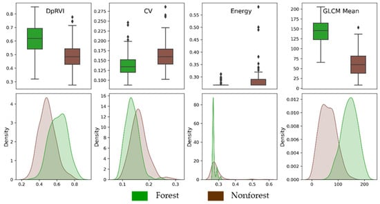
Figure 5.
Boxplots and kernel density estimates of GLCM texture measures derived from DpRVI to distinguish between forest and nonforest study classes. DpRVI is the starting L-band radar measure from which each texture measure is derived. DpRVI values range from 0 to 1 while measures of texture are unitless. The GLCM mean texture measure demonstrates the greatest separability between the forest and nonforest classes. In contrast, the coefficient of variation (CV) and energy texture measures show reduced separability between these classes compared to using DpRVI alone.
3.2. Full-Polarimetry and Dual-Polarimetry Classifications
We trained a random forest classifier to assess the effectiveness of full-pol and dual-pol L-band radar measures, along with their derived GLCMm texture features, in distinguishing between Lowland Chocó nonforest and forest classes. Table 5 summarizes the main classification results obtained from approaches utilizing the full-pol and dual-pol radar measures, along with their associated GLCMm features derived from the reference 2015 PALSAR-2 scene. In total, we analyzed 10,183 spatially validated pixel samples, derived from field-confirmed forest and nonforest sites, for use in training and evaluating all classification approaches presented in this study. The FpFD approach was configured with two input variables for classification, i.e., VSPN and SSPN, while the RVI and DpRVI approaches were configured to use these indices as the sole input variables, as shown in Table 3. The texture-based approaches were configured to use the GLCMm feature as the sole input variable for classification. For the FpFD GLCMm approach, both VSPN GLCMm and SSPN GLCMm were included as input variables. A summary of the classification approaches examined in this study is provided in Table 3. The individual confusion matrices with all accuracy measures are provided in Appendix B.
Table 5.
Validation results for distinguishing between forest and nonforest areas in the testing data, comparing classification approaches using radar measures and their associated GLCM mean texture statistics, all derived from the 2015 L-band PALSAR-2 reference scene. The top section presents results where each radar measure was used independently as the sole input feature, while the bottom section shows results based on texture (GLCM mean) of each radar measure.
The results demonstrated that utilization of GLCMm texture features as classification input variables improved the user, producer, and overall accuracy across all classifiers (Table 5). Without the GLCMm as an input variable, only the forest class user and producer accuracies exceeded 90%. The nonforest user accuracy in the FpFD approach was 80.9%, and considerably lower in the RVI and DpRVI classifiers (49.2% and 35.9%). Notably, substituting the GLCMm texture feature as a classification input variable greatly improved both nonforest user and producer accuracies across all approaches, and most particularly for the DpRVI. Importantly, these results surpassed the accuracies achieved by the FpFD approach without the GLCMm as a classification input variable. When substituting the DpRVI GLCMm for the DpRVI as the classification input variable, we observed a substantial user accuracy increase from 35.9% to 86.3%, producer accuracy increase from 31.7% to 83.0%, and overall accuracy increase from 88.2% to 97.2%, which was comparable to the FpFD GLCMm classification overall accuracy (97.7%). Additionally, a key finding was that the single-predictor random forest model (DpRVI GLCMm) outperformed the two-predictor model (FpFD GLCMm) in terms of nonforest producer accuracy (83.0% versus 79.2%).
We employed these classifiers to develop forest/nonforest maps of the Lowland Chocó region, covering the full 182 km2 study area, and visually assessed the impact of texture inclusion in each approach (Figure 6). We observed that the forest/nonforest maps generated using only the radar measures, i.e., FpFD, RVI, and DpRVI, without the inclusion of derived GLCMm texture features, exhibited numerous isolated nonforest areas scattered across the maps. (Figure 6, left panels). However, those results are not corroborated by ground validation. In contrast, the forest/nonforest maps incorporating GLCMm-derived texture features exhibit spatial patterns that are more consistent with field-validated degradation history and known land-use trajectories in the study region (Figure 6, right panels). This improvement is especially evident in the reduction in pixelated noise and greater contiguity of deforested patches, which better reflect the ecological and spatial dynamics of forest degradation observed during our field campaigns
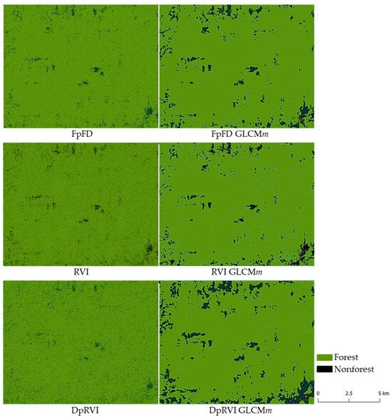
Figure 6.
Forest and nonforest classification results for the Lowland Chocó study area based on the 2015 PALSAR-2 full-polarimetric (full-pol) and dual-polarimetric (dual-pol) imagery. Left panels show classification results using only radar intensity and polarimetric indices (e.g., RVI, DpRVI), while right panels include GLCM mean texture features derived from the same radar inputs. Incorporating GLCMm improves classification performance by reducing speckle noise, suppressing pixel-level misclassification artifacts, and improving delineation of deforested areas.
We also evaluated the precision of each approach using GLCMm-derived features by examining the agreement between the forest/nonforest classification maps at the pixel level. We found the pixel-wise agreement to exceed 97.5% for all forest/nonforest maps produced with the GLCMm-derived features. The FpFD GLCMm approach classified a greater number of pixels as nonforest compared to the DpRVI GLCMm approach. This resulted in the identification of 16,762.6 hectares of forest in the FpFD GLCMm approach compared to 16,964.9 hectares of forest in the DpRVI GLCMm approach. Additionally, the FpFD GLCMm approach classified 1377.9 hectares of nonforest, while the DpRVI GLCMm approach classified 1182.0 hectares of nonforest. We noted that classification disagreements were most prevalent along the forest/nonforest boundaries, while both approaches consistently identified the interior regions of nonforest patches.
3.3. Temporal Analysis of Regenerating Forest
To monitor the chronosequence of natural regeneration from pasture and cacao to forest plots, we first characterized the end-member classes, i.e., active pasture, active cacao, and forest classes, using time series PALSAR and PALSAR-2 observations spanning the 12-year study period (Table 1). The characterization of the class means as a function of the radar vegetative indices, i.e., RFDI, DpRVI, as well as RFRI, for each year indicated that the fixed pasture, cacao, and forest classes remained effectively stable classes during the 12-year PALSAR and PALSAR-2 observation period (Figure 7). The L-band mean values for each fixed class are provided in Table 6.
Figure 7.
Comparison of the fixed landcover classes across the PALSAR and PALSAR-2 L-band study period as a function of the vegetation indices (A) RFDI, (B) DpRVI, and (C) RFRI. Distributions are ±1 standard deviation for each point.
Table 6.
Average L-band SAR measures by land cover class for the Lowland Chocó study area, derived from PALSAR and PALSAR-2 time series data. The pasture, cacao, and forest classes are static throughout the study period. Regenerating pasture and cacao classes represent dynamic plots along a post-disturbance regrowth chronosequence spanning 0–35 years since conservation.
We also characterized the regenerating cacao and pasture classes over the chronosequence and at different stages of forest recovery. In Figure 8, we show a selection of plots from each regenerating class that span the REASSEMBLY project chronosequence. For the plots in the early forest successional stages (PR25 and CR02, Appendix A), we included data before the conservation protection date that correlate with the start of natural regeneration to characterize the transition from fixed to regenerating classes. The older plots within each regenerating class along the chronosequence (PR21 and CR14, Appendix A) attained RFRI values typical of forested areas.
Figure 8.
Selection of pasture regeneration (PR) and cacao regeneration (CR) plots along the REASSEMBLY project chronosequence. Plots begin with natural forest recovery near regeneration year = 0. Negative regeneration years correspond with PALSAR and PALSAR-2 observations prior to the plot achieving conservation status. Distributions are ±1 standard deviation for each point.
We developed a complete recovery chronosequence for each class by aggregating mean L-band measures across plots of a known regeneration age (Figure 9). This space-for-time substitution approach enables inferences on forest structural recovery trajectories over time. While displayed the most dynamic range within the regenerating classes, only the RFRI demonstrated both the consistency and sensitivity needed to differentiate between all landcover classes within the study area (Table 6).
Figure 9.
Chronosequence of structural recovery in regenerating pasture and cacao plots toward forest conditions. Each point represents the mean L-band measure for a given regeneration year, aggregated across plots within a land-use class. Error bars denote ±1 standard deviation. Negative regeneration years represent PALSAR and PALSAR-2 observations taken prior to the initiation of forest regeneration (i.e., prior to conservation status), capturing static land-use conditions (e.g., active pasture or cacao cultivation).
We extended the analysis beyond the validation plots to classify transitional forest regions in the Lowland Chocó. We developed a final classification map using the time series RFRI derivations spanning the years 2007–2019 (Figure 10). Table 7 provides the confusion matrix and main validation results for the transitional forest classification. The user accuracies were very high across all three classes; however, the producer accuracy for the transitional forest class was notably lower than the forest and nonforest classes. We attributed this to the dynamic nature of the transitional forest training class, which includes both regenerating pasture and regenerating cacao data, spanning a significant portion of the recovery chronosequence. Even with our conservative approach of excluding data from the youngest and oldest stages, individual sites within this class may align more closely with a fixed category, such as pasture or forest, depending on the specific plot characteristics and the regeneration year of each training pixel in a given PALSAR or PALSAR-2 scene. Nonetheless, the overall accuracy (95.5%) remained high due to the large proportion of forest regions in the study area, and most importantly, the classification map reasonably identified transitioning forest regions at the interface between forest and nonforest areas.
Figure 10.
Classification map including transitioning forest areas developed using RFRI generated from the 12-year time series of PALSAR and PALSAR-2 imagery acquired between 2007 and 2019.
Table 7.
Confusion matrix for transitional forest map developed using a time series (2007–2019) RFRI stack as classification features. Map classes are the rows and reference classes are the columns.
4. Discussion
We demonstrated that incorporating gray-level co-occurrence matrix (GLCM) texture measures derived from dual-polarimetric (HH, HV) L-band PALSAR and PALSAR-2 imagery improves separability between forest and nonforest classes under topographically complex tropical conditions. These results are based on a single-date (2015) image analysis and show consistent improvements in classification performance when GLCM mean texture features are included. In our analysis, we found that the GLCM mean texture derived from the DpRVI was the most effective measure for distinguishing between forest and nonforest classes (F1,446 = 756; p < 0.0005), outperforming the original DpRVI product by over 450 points (F1,446 = 172; p < 0.0005). However, not all texture measures enhanced classification performance. Common texture measures such as contrast, energy, and homogeneity were less effective in distinguishing between classes (F1,446 < 70; p > 0.0005) compared to the original DpRVI product from which they were derived.
Interestingly, texture measures derived from the DpRVI outperformed those derived from the full-polarimetric RVI in distinguishing between forest and nonforest classes (Table 4). This suggests that while the RVI is based on full-pol data, its reliance on intensity-only terms limits its sensitivity when used as a precursor to textural analysis. In contrast, the DpRVI, though based on dual-pol data, incorporates more nuanced structural information through decomposition techniques and preserves complex data characteristics. When paired with GLCM-based texture derivation, this approach results in a higher capacity to capture spatial heterogeneity associated with forest degradation and disturbance. These findings support the notion that combining polarimetric decomposition with spatial texture analysis offers a more powerful method for forest classification than relying on intensity-derived indices alone.
Building on this, the present study contributes to a well-established body of research demonstrating the practical application of radar image textures for classifying tropical land cover and evaluating forest conditions, including studies using both L-band and C-band SAR data [21,22,23,53,54,55,56]. Here, we advanced this research by developing a random forest classifier using image textures derived from the polarimetric decomposition of dual-pol PALSAR-2 imagery (i.e., DpRVI), which demonstrated a comparable classification accuracy to our approach using the Freeman–Durden decomposition of full-pol PALSAR-2 imagery.
The confusion matrix results showed that employing dual-pol decomposition and subsequently deriving the GLCM mean from the DpRVI substantially improved the user, producer, and overall forest/nonforest classification accuracy (user accuracy improved from 35.9% to 86.3%, producer accuracy from 31.7% to 83.0%, and overall accuracy from 88.2% to 97.2%). These improvements were comparable to the results obtained using the Freeman–Durden decomposition product and subsequent derivation of the GLCM mean in the classification process. Notably, the DpRVI GLCMm model outperformed the two-feature FpFD GLCMm model in nonforest producer accuracy (83.0% vs. 79.2%), highlighting its potential for the improved detection of nonforest areas, which can be critical for monitoring deforestation and degradation fronts. Although the DpRVI exhibited the highest ANOVA F-scores (Table 4), indicating strong univariate class separability between forest and nonforest classes, this did not directly translate to the highest overall classification accuracy in the single-feature models (Table 5). In contrast, the combined use of SSPN and VSPN in the FpFD model—a pair of complementary full-pol decomposition parameters representing surface and volume scattering, respectively—yielded a better overall classification accuracy. This result underscores the advantage of multivariate input, where the combination of structurally informative features captures a broader range of scattering behaviors and forest condition variability than any single index alone.
These findings suggest that dual-pol L-band SAR, when combined with appropriate decomposition and texture measures, can serve as a powerful alternative to full-pol approaches. This is particularly important for tropical forest monitoring in regions where full-polarimetric acquisitions are limited or unavailable. Employing decomposition followed by texture derivation from complex dual-pol data produced consistently higher classification accuracies than methods based solely on intensity-based full-pol indices like the RVI, demonstrating the utility of structural and contextual backscatter measures in operational forest/nonforest mapping frameworks.
When employing these classifications to develop regional forest/nonforest maps, we observed a strong agreement between the maps originating from the full-pol and dual-pol decomposition approaches. Discrepancies between the maps were primarily evident at the boundaries between forest and nonforest areas. However, all classifications based on a GLCM mean derivation accurately identified the locations of nonforest patches, corroborated by ground validation of historical deforestation patterns in the Lowland Chocó. This finding is significant, as it demonstrates the utility of complex dual-polarized L-band data, which are more readily available temporally compared to fully-polarimetric imagery, for identifying deforestation activities in near real-time alert systems.
We utilized the more frequent acquisition dual-pol imagery to expand our analysis and propose a method for monitoring natural forest regeneration in tropical conservation areas by tracking changes in image texture over time. By normalizing time series DpRVI GLCM mean images to a common scale, we developed a new metric termed the Radar Forest Regeneration Index (RFRI). Our approach proved effective in the Lowland Chocó and can serve as a model for application in other ecoregions. Typically, measures of image textures are used to make regional comparisons within a single scene or date. However, within the tropical regions considered in this study, we observed that the image texture of fixed land cover classes, i.e., areas where land cover conversion did not occur during the study period, remained relatively stable over time. The stability of the fixed forest, pasture, and cacao classes in this study was corroborated by analyzing two vegetation indices, i.e., RFDI and DpRVI values, for each of these active classes over our 12-year PALSAR and PALSAR-2 observation period (Figure 7). The slight changes observed during this period, such as a minor increase in the cacao RFDI and a decrease in the forest RFDI, along with the corresponding opposite changes in the DpRVI, were attributed to the status of active classes and do not necessarily imply that no changes over time occurred. Cacao is periodically harvested and thus experiences different human management impacts across plots. Active pasture sites undergo cycles of impact from livestock grazing. While the forest sites in this study are considered mature, few untouched forests remain in this location due to historical human interventions. Therefore, we expected these forest areas to continue to grow and accumulate biomass over time, indicated by an increase in the DpRVI and a decrease in the RFDI.
Our description of forest regeneration focused primarily on experimental regenerating pasture plots and regenerating cacao plots at various stages of forest regrowth along a chronosequence. At the level of individual plots, we observed more pronounced changes in the RFRI for the regenerating pasture plots compared to the regenerating cacao plots. This discrepancy can be attributed to several factors. Theobroma cacao, a small evergreen tree native to tropical America, is industrially cultivated in monoculture plantations. However, cacao is also a natural shade crop that can thrive under an established forest canopy. In our Lowland Chocó study region, industrial cacao plantations are absent, and instead, small landholders and subsistence farmers often establish mixed agricultural plots. This leads to a diversity of cultivation strategies at the small plot scale, with cacao also planted opportunistically within a mixed forest setting.
Active cacao RFRI values surpassed those of pastures, which typically feature more uniform open fields and sparse tree cover with predominating grasses. We hypothesize that young pasture regeneration plots, initially characterized by open canopy areas, facilitate rapid colonization by pioneer species in early regeneration years, resulting in significant textural changes within plots compared to regenerating cacao plots, which already harbor established evergreen cacao trees. Regenerating cacao sites exhibit more diverse vegetation communities with more developed canopy structures, leading to greater variations in tree age, standing biomass, and canopy height across sites (Figure 2). These factors may impede the rapid growth and success commonly observed in pasture regeneration [57,58]. Moreover, determining the number of years of natural regeneration for a specific plot can be challenging in some instances due to complications arising from land deed transfers, which are often complex processes in tropical forest regions. Additionally, degradation may persist even after a plot attains a protected status. For instance, some plots may have been abandoned before being acquired by conservation groups and may have already undergone some degree of natural regeneration at the time of acquisition. Conversely, other plots may continue to be utilized, such as for opportunistic pasture areas by subsistence farmers. In the early years following purchase, monitoring efforts and land transfers are often difficult in these remote, subsistence-driven regions.
Nevertheless, considering regeneration at the aggregate class level (Figure 9) revealed that both regenerating pasture and regenerating cacao plots gradually approached the RFRI texture characteristic of forests over a period of approximately 20 years in the natural regeneration chronosequence. This timeline corresponds with separate assessments of tropical forest structural recovery [59,60]. Our findings indicate that the RFRI ranges from less than 0.4 for nonforest regions, between 0.4 and 0.6 for regenerating forests, and 0.6 and greater for mature forests. While we recognize that this range of index values is comparable to the RFDI; the results from our distinct RFRI derivation approach suggest that the RFRI exhibits greater sensitivity to regenerating forests originating from pasture and cacao areas in the study region. Although all L-band measures could to some extent differentiate between forest and nonforest classes, only the RFRI demonstrated the necessary sensitivity to distinguish between the active pasture, active cacao, regenerating pasture, and regenerating cacao classes. This indicates that the RFRI is likely more suitable for monitoring temporal changes in forest recovery and degradation. This is particularly valuable for the type of forest–agricultural matrix observed in the Canandé area, which is typical of regions at the deforestation frontier. It is important to note that our approach here does not aim to establish the absolute values of any measurement. Instead, we offer ranges for each measure that serve as indicators of representative tropical forest land cover types, aiding in land cover classification and the assessment of forest regrowth.
Our analysis was based on a local study and may need customization for applications in other ecoregions. While our classification results reveal spatial patterns that align closely with field observations and known land-use trajectories, it is important to acknowledge potential sources of uncertainty in our analysis. These uncertainties arise from both methodological choices and environmental variability, and although we have taken multiple steps to mitigate them, some level of classification error is unavoidable.
Differences in spatial resolution, polarization mode, and acquisition geometry between PALSAR and PALSAR-2 may affect radiometric consistency across the time series. To reduce these effects, we employed measures derived from HH and HV channels, which ensured comparability between sensors. Nonetheless, slight discrepancies—particularly near forest edge boundaries—may still contribute to classification noise. We also recognize the potential impact of temporal variation. Year-to-year variability in vegetation moisture, soil conditions, and local land-use practices may still affect radar backscatter and texture measures. These fluctuations could influence classification performance in transitional or regenerating areas, where surface conditions are more dynamic.
In terms of class distribution, our reference dataset reflects the forest-dominated composition of the landscape, resulting in an imbalance with a greater proportion of forest pixels (~90%). We addressed this by applying balanced class weighting within the random forest classifier, which helps reduce bias during training. However, some residual skew may persist, particularly in mixed or marginal areas near class boundaries. Furthermore, the training dataset, while grounded in field-validated plots and corroborated with optical imagery, was influenced by accessibility constraints, which may have introduced a spatial sampling bias. To reduce this risk, we supplemented our training pool with manually verified areas across a broader extent of the study region, ensuring that multiple forest conditions and disturbance regimes were represented.
While the use of GLCM-based texture features clearly improved classification performance in heterogeneous landscapes, these features are sensitive to design parameters such as window size, quantization level, and kernel configuration. We standardized these parameters across all classifications to maintain consistency, but some degree of variability may still occur due to differences in underlying scene structure. However, we are confident that considering the texture at the landscape scale can significantly improve global forest monitoring efforts with L-band SAR.
A current limitation to the wider evaluation of our approaches is the availability of suitable L-band imagery. ALOS/PALSAR provided data at a 46-day nominal revisit with varying acquisition modes, while PALSAR-2 improves this to a 14-day cycle; however, the high-resolution PALSAR-2 imagery is not openly accessible. Although open-access PALSAR-2 ScanSAR data provide increased temporal coverage post-2016, their coarser spatial resolution (~100 m) lacks continuity with earlier ALOS/PALSAR acquisitions, limiting its utility for fine-scale, long-term ecological studies such as this one. A key factor in overcoming this challenge is the upcoming NISAR mission. NISAR will bring two crucial improvements over currently openly available SAR-based satellite missions: more frequent revisit times (approximately every 6 days) and simultaneous L-band and S-band acquisitions over India and across the globally distributed NISAR cal/val sites. This more robust time series will better facilitate the calibration of land cover textures over time. Additionally, the simultaneous acquisitions from dual radar wavelengths at multiple polarizations will allow for a more comprehensive characterization of various vegetation structural parameters, such as canopy structure and biomass, which will further aid in the identification of different tropical forest vegetation types. Furthermore, the open-access nature, consistent global acquisitions, and high spatial resolution of NISAR (≥10 m) represent a significant advancement in the operational monitoring of tropical forest degradation and recovery. These capabilities are expected to improve the ability of end-users to detect and map subtle disturbances such as selective logging, which remain challenging to capture in near real time with current SAR-based approaches. Our analysis serves as a foundation upon which the NISAR mission can build and improve. Our results indicate that the expected increase in the availability of SAR data from NISAR will greatly advance research in tropical forest ecosystems and biodiversity conservation applications.
5. Conclusions
We demonstrated that specific texture features derived from the GLCM analysis of complex dual-pol L-band PALSAR and PALSAR-2 imagery can significantly improve the detection of forest and nonforest areas, enhancing the overall classification performance by nearly 10%. We found that the GLCM mean texture was most effective in distinguishing between tropical forest land cover classes. Furthermore, we developed a random forest classifier using texture features derived from dual-pol L-band PALSAR-2 imagery, which showed a comparable classification accuracy to methods using full-pol imagery.
We proposed a method that enhanced the monitoring of natural forest regeneration in tropical conservation areas by tracking changes in the image texture over time. We introduced a new metric, the Radar Forest Regeneration Index (RFRI), derived from a time series of DpRVI GLCM mean normalized images. This metric demonstrated improved sensitivity in distinguishing between active pasture, active cacao, regenerating pasture, regenerating cacao, and old-growth forest classes compared to , , DpRVI, and RFDI. Our findings from the Lowland Chocó region can be applied to other ecoregions, providing valuable insights into tropical forest land cover types. Our approach does not aim to establish absolute RFRI values but rather offers ranges as indicators for land cover classification and forest regrowth assessment. Looking ahead, the upcoming NISAR mission, with more frequent revisit times and simultaneous L-band and S-band acquisitions over select regions, holds promise for revolutionizing tropical forest monitoring. This will allow for a better characterization of land cover textures over time, ultimately advancing research in tropical forest ecosystems and biodiversity conservation.
Author Contributions
Conceptualization, D.S.T. and K.C.M.; data curation, D.S.T., C.J.T., F.L.N. and E.V.-G.; investigation, D.S.T., C.J.T., F.L.N. and N.B.; methodology, D.S.T., E.P., K.C.M. and B.T.L.; software, D.S.T.; formal analysis, D.S.T. and K.C.M.; visualization, D.S.T.; validation, D.S.T., C.J.T., F.L.N., E.V.-G., N.B., R.N. and H.M.S.; supervision, K.C.M., N.B. and H.M.S.; writing—original draft preparation, D.S.T.; writing—review and editing, all authors. All authors have read and agreed to the published version of the manuscript.
Funding
Portions of this research were supported by a grant under the NASA NISAR Science Team (grant 80NSSC19K1513).
Data Availability Statement
Datasets and classification products from this study are available upon request by contacting the authors.
Acknowledgments
Portions of this work were carried out at the Jet Propulsion Laboratory, California Institute of Technology, under contract with the National Aeronautics and Space Administration. ALOS PALSAR data were provided by the Alaska Satellite Facility DAAC under JAXA’s open data policy. ALOS-2 PALSAR-2 data were provided through the Kyoto and Carbon Initiative under a limited-use research agreement with JAXA. We gratefully acknowledge their support in enabling this work.
Conflicts of Interest
The authors declare no conflicts of interest.
Appendix A
Table A1.
Validation plots in the Lowland Chocó utilized in this study. Regeneration year denotes the year when a site was acquired for conservation purposes, marking the approximate starting point of natural forest regeneration. Classes without regeneration year (-) are fixed classes through the PALSAR AND PALSAR-2 observation period (2007–2019). Plots with regeneration years after the observation period are considered active classes in this study. All plots are approximately 50 × 50 m.
| Plot | Class | Regeneration Year |
|---|---|---|
| CA59 | Cacao | - |
| CA60 | Cacao | - |
| CA61 | Cacao | - |
| CA62 | Cacao | - |
| CA63 | Cacao | - |
| CA64 | Cacao | - |
| CR13 | Cacao | 2022 |
| OG28 | Old-growth Forest | - |
| OG37 | Old-growth Forest | - |
| OG38 | Old-growth Forest | - |
| OG39 | Old-growth Forest | - |
| OG40 | Old-growth Forest | - |
| OG41 | Old-growth Forest | - |
| OG42 | Old-growth Forest | - |
| OG43 | Old-growth Forest | - |
| OG44 | Old-growth Forest | - |
| OG45 | Old-growth Forest | - |
| OG46 | Old-growth Forest | - |
| OG47 | Old-growth Forest | - |
| OG48 | Old-growth Forest | - |
| OG49 | Old-growth Forest | - |
| OG50 | Old-growth Forest | - |
| OG51 | Old-growth Forest | - |
| OG52 | Old-growth Forest | - |
| PA53 | Pasture | - |
| PA54 | Pasture | - |
| PA55 | Pasture | - |
| PA56 | Pasture | - |
| PA57 | Pasture | - |
| PA58 | Pasture | - |
| PR20 | Pasture | 2019 |
| PR33 | Pasture | 2022 |
| CR01 | Regenerating Cacao | 2017 |
| CR02 | Regenerating Cacao | 2015 |
| CR03 | Regenerating Cacao | 2018 |
| CR04 | Regenerating Cacao | 2002 |
| CR05 | Regenerating Cacao | 2011 |
| CR06 | Regenerating Cacao | 2003 |
| CR07 | Regenerating Cacao | 2000 |
| CR08 | Regenerating Cacao | 1996 |
| CR09 | Regenerating Cacao | 2017 |
| CR10 | Regenerating Cacao | 1999 |
| CR11 | Regenerating Cacao | 1992 |
| CR12 | Regenerating Cacao | 2008 |
| CR14 | Regenerating Cacao | 1985 |
| CR15 | Regenerating Cacao | 2015 |
| CR16 | Regenerating Cacao | 2015 |
| CR17 | Regenerating Cacao | 2014 |
| CR18 | Regenerating Cacao | 2013 |
| PR19 | Regenerating Pasture | 2017 |
| PR21 | Regenerating Pasture | 1987 |
| PR22 | Regenerating Pasture | 2011 |
| PR23 | Regenerating Pasture | 2022 |
| PR24 | Regenerating Pasture | 2002 |
| PR25 | Regenerating Pasture | 2017 |
| PR26 | Regenerating Pasture | 2001 |
| PR27 | Regenerating Pasture | 1996 |
| PR29 | Regenerating Pasture | 2017 |
| PR30 | Regenerating Pasture | 2008 |
| PR31 | Regenerating Pasture | 1999 |
| PR32 | Regenerating Pasture | 1997 |
| PR34 | Regenerating Pasture | 1985 |
| PR35 | Regenerating Pasture | 2016 |
| PR36 | Regenerating Pasture | 2014 |
The standard measures of texture computed and assessed in this study, where µ is the mean pixel value; σ is the standard deviation; i is the GLCM row number; j is the column number; Pi,j is the probability value recorded for the cell i, j; and N is the number of rows or columns of the GLCM. We derived each texture statistic with the following parameters: all angles from the center pixel (45°, 90°, 135°, 0°), 3-pixel displacement, 64-bit gray-level quantization, and 5 × 5 window size.
Appendix B
This appendix provides the comprehensive accuracy assessment results presented in tables. Each table consists of two sections: the upper section displays the plot-based confusion matrix, while the lower section presents the confusion matrix with the corresponding aggregated weights of the plots. Map categories are the rows and reference categories are the columns.
Table A2.
Confusion matrix for 2015 FNF map developed from FpFD, VSPN, and SSPN bands as classification features. Map classes are the rows and reference classes are the columns.
Table A2.
Confusion matrix for 2015 FNF map developed from FpFD, VSPN, and SSPN bands as classification features. Map classes are the rows and reference classes are the columns.
| Class | Forest | Nonforest | Total | Map Area (ha) | Weights | ||||
|---|---|---|---|---|---|---|---|---|---|
| Forest | 9113 | 110 | 9223 | 144 | 0.906 | ||||
| Nonforest | 494 | 466 | 960 | 15 | 0.094 | ||||
| Total | 9607 | 576 | 10,183 | 159 | 1.000 | ||||
| Class | Forest | Nonforest | Total | User | CI at 95% | Producer | CI at 95% | Overall | CI at 95% |
| Forest | 0.895 | 0.011 | 0.906 | 0.949 | ±0.0086 | 0.988 | ±0.0043 | 0.941 | ±0.0091 |
| Nonforest | 0.049 | 0.046 | 0.094 | 0.809 | ±0.0613 | 0.485 | ±0.0624 | ||
| Total | 0.943 | 0.057 | 1.000 |
Table A3.
Confusion matrix for 2015 FNF map developed from FpFD, VSPN, and SSPN GLCMm bands as classification features. Map classes are the rows and reference classes are the columns.
Table A3.
Confusion matrix for 2015 FNF map developed from FpFD, VSPN, and SSPN GLCMm bands as classification features. Map classes are the rows and reference classes are the columns.
| Class | Forest | Nonforest | Total | Map Area (ha) | Weights | ||||
|---|---|---|---|---|---|---|---|---|---|
| Forest | 9188 | 35 | 9223 | 144 | 0.906 | ||||
| Nonforest | 200 | 760 | 960 | 15 | 0.094 | ||||
| Total | 9388 | 795 | 10,183 | 159 | 1.000 | ||||
| Class | Forest | Nonforest | Total | User | CI at 95% | Producer | CI at 95% | Overall | CI at 95% |
| Forest | 0.902 | 0.003 | 0.906 | 0.979 | ±0.0057 | 0.996 | ±0.0025 | 0.977 | ±0.0056 |
| Nonforest | 0.020 | 0.075 | 0.094 | 0.956 | ±0.0286 | 0.792 | ±0.0475 | ||
| Total | 0.922 | 0.078 | 1.000 |
Table A4.
Confusion matrix for 2015 FNF map developed from RVI as classification feature. Map classes are the rows and reference classes are the columns.
Table A4.
Confusion matrix for 2015 FNF map developed from RVI as classification feature. Map classes are the rows and reference classes are the columns.
| Class | Forest | Nonforest | Total | Map Area (ha) | Weights | ||||
|---|---|---|---|---|---|---|---|---|---|
| Forest | 8828 | 395 | 9223 | 144 | 0.906 | ||||
| Nonforest | 577 | 383 | 960 | 15 | 0.094 | ||||
| Total | 9405 | 778 | 10,183 | 159 | 1.000 | ||||
| Class | Forest | Nonforest | Total | User | CI at 95% | Producer | CI at 95% | Overall | CI at 95% |
| Forest | 0.867 | 0.039 | 0.906 | 0.939 | ±0.0099 | 0.957 | ±0.0079 | 0.905 | ±0.0116 |
| Nonforest | 0.057 | 0.038 | 0.094 | 0.492 | ±0.0677 | 0.399 | ±0.0646 | ||
| Total | 0.924 | 0.076 | 1.000 |
Table A5.
Confusion matrix for 2015 FNF map developed from RVI GLCMm as classification feature. Map classes are the rows and reference classes are the columns.
Table A5.
Confusion matrix for 2015 FNF map developed from RVI GLCMm as classification feature. Map classes are the rows and reference classes are the columns.
| Class | Forest | Nonforest | Total | Map Area (ha) | Weights | ||||
|---|---|---|---|---|---|---|---|---|---|
| Forest | 9038 | 185 | 9223 | 144 | 0.906 | ||||
| Nonforest | 264 | 696 | 960 | 15 | 0.094 | ||||
| Total | 9302 | 881 | 10,183 | 159 | 1.000 | ||||
| Class | Forest | Nonforest | Total | User | CI at 95% | Producer | CI at 95% | Overall | CI at 95% |
| Forest | 0.888 | 0.018 | 0.906 | 0.972 | ±0.0068 | 0.980 | ±0.0056 | 0.956 | ±0.0087 |
| Nonforest | 0.026 | 0.068 | 0.094 | 0.790 | ±0.0509 | 0.725 | ±0.0574 | ||
| Total | 0.913 | 0.087 | 1.000 |
Table A6.
Confusion matrix for 2015 FNF map developed from DpRVI as classification feature. Map classes are the rows and reference classes are the columns.
Table A6.
Confusion matrix for 2015 FNF map developed from DpRVI as classification feature. Map classes are the rows and reference classes are the columns.
| Class | Forest | Nonforest | Total | Map Area (ha) | Weights | ||||
|---|---|---|---|---|---|---|---|---|---|
| Forest | 8681 | 542 | 9223 | 144 | 0.906 | ||||
| Nonforest | 656 | 304 | 960 | 15 | 0.094 | ||||
| Total | 9337 | 846 | 10,183 | 159 | 1.000 | ||||
| Class | Forest | Nonforest | Total | User | CI at 95% | Producer | CI at 95% | Overall | CI at 95% |
| Forest | 0.852 | 0.053 | 0.906 | 0.93 | ±0.0102 | 0.941 | ±0.0095 | 0.882 | ±0.0124 |
| Nonforest | 0.064 | 0.030 | 0.094 | 0.359 | ±0.0651 | 0.317 | ±0.0607 | ||
| Total | 0.917 | 0.083 | 1.000 |
Table A7.
Confusion matrix for 2015 FNF map developed from DpRVI GLCMm as classification feature. Map classes are the rows and classes categories are the columns.
Table A7.
Confusion matrix for 2015 FNF map developed from DpRVI GLCMm as classification feature. Map classes are the rows and classes categories are the columns.
| Class | Forest | Nonforest | Total | Map Area (ha) | Weights | ||||
|---|---|---|---|---|---|---|---|---|---|
| Forest | 9097 | 126 | 9223 | 144 | 0.906 | ||||
| Nonforest | 163 | 797 | 960 | 15 | 0.094 | ||||
| Total | 9260 | 923 | 10,183 | 159 | 1.000 | ||||
| Class | Forest | Nonforest | Total | User | CI at 95% | Producer | CI at 95% | Overall | CI at 95% |
| Forest | 0.893 | 0.012 | 0.906 | 0.982 | ±0.0053 | 0.986 | ±0.0047 | 0.972 | ±0.0063 |
| Nonforest | 0.016 | 0.078 | 0.094 | 0.863 | ±0.0435 | 0.83 | ±0.0472 | ||
| Total | 0.909 | 0.091 | 1.000 |
References
- Christensen, N.L.; Bartuska, A.M.; Brown, J.H.; Carpenter, S.; D’Antonio, C.; Francis, R.; Franklin, J.F.; MacMahon, J.A.; Noss, R.F.; Parsons, D.J.; et al. The Report of the Ecological Society of America Committee on the Scientific Basis for Ecosystem Management. Ecol. Appl. 1996, 6, 665–691. [Google Scholar] [CrossRef]
- Shugart, H.H.; Saatchi, S.; Hall, F.G. Importance of Structure and Its Measurement in Quantifying Function of Forest Ecosystems. J. Geophys. Res. 2010, 115, 2009JG000993. [Google Scholar] [CrossRef]
- Arroyo-Rodríguez, V.; Dias, P.A.D. Effects of Habitat Fragmentation and Disturbance on Howler Monkeys: A Review. Am. J. Primatol. 2010, 72, 1–16. [Google Scholar] [CrossRef] [PubMed]
- Martínez-Ramos, M.; Ortiz-Rodríguez, I.A.; Piñero, D.; Dirzo, R.; Sarukhán, J. Anthropogenic Disturbances Jeopardize Biodiversity Conservation within Tropical Rainforest Reserves. Proc. Natl. Acad. Sci. USA 2016, 113, 5323–5328. [Google Scholar] [CrossRef]
- Noss, R.F. Indicators for Monitoring Biodiversity: A Hierarchical Approach. Conserv. Biol. 1990, 4, 355–364. [Google Scholar] [CrossRef]
- Cook-Patton, S.C.; Leavitt, S.M.; Gibbs, D.; Harris, N.L.; Lister, K.; Anderson-Teixeira, K.J.; Briggs, R.D.; Chazdon, R.L.; Crowther, T.W.; Ellis, P.W.; et al. Mapping Carbon Accumulation Potential from Global Natural Forest Regrowth. Nature 2020, 585, 545–550. [Google Scholar] [CrossRef]
- Hyde, P.; Dubayah, R.; Walker, W.; Blair, J.B.; Hofton, M.; Hunsaker, C. Mapping Forest Structure for Wildlife Habitat Analysis Using Multi-Sensor (LiDAR, SAR/InSAR, ETM+, Quickbird) Synergy. Remote Sens. Environ. 2006, 102, 63–73. [Google Scholar] [CrossRef]
- Hansen, M.C.; Potapov, P.V.; Moore, R.; Hancher, M.; Turubanova, S.A.; Tyukavina, A.; Thau, D.; Stehman, S.V.; Goetz, S.J.; Loveland, T.R.; et al. High-Resolution Global Maps of 21st-Century Forest Cover Change. Science 2013, 342, 850–853. [Google Scholar] [CrossRef]
- Bullock, E.L.; Woodcock, C.E.; Olofsson, P. Monitoring Tropical Forest Degradation Using Spectral Unmixing and Landsat Time Series Analysis. Remote Sens. Environ. 2020, 238, 110968. [Google Scholar] [CrossRef]
- Flores, A.; Herndon, K.; Thapa, R.; Cherrington, E. Synthetic Aperture Radar (SAR) Handbook: Comprehensive Methodologies for Forest Monitoring and Biomass Estimation; Alabama University: Huntsville, AL, USA, 2019. [Google Scholar] [CrossRef]
- Hirschmugl, M.; Deutscher, J.; Sobe, C.; Bouvet, A.; Mermoz, S.; Schardt, M. Use of SAR and Optical Time Series for Tropical Forest Disturbance Mapping. Remote Sens. 2020, 12, 727. [Google Scholar] [CrossRef]
- Ulaby, F.T.; Fung, A.K.; Dobson, M.C.; Cihlar, J. Evaluation of the Radar Response to Land Surfaces and Volumes: Examination of Theoretical Models, Target Statistics, and Applications. In The Shuttle Imaging Radar-B Science Investigation Plan; ADS: Carrollton, TX, USA, 1984. [Google Scholar]
- Barrett, B.; Dwyer, E.; Whelan, P. Soil Moisture Retrieval from Active Spaceborne Microwave Observations: An Evaluation of Current Techniques. Remote Sens. 2009, 1, 210–242. [Google Scholar] [CrossRef]
- Trisasongko, B.H. The Use of Polarimetric SAR Data for Forest Disturbance Monitoring. Sens. Imaging 2010, 11, 1–13. [Google Scholar] [CrossRef]
- Shimada, M.; Itoh, T.; Motooka, T.; Watanabe, M.; Shiraishi, T.; Thapa, R.; Lucas, R. New Global Forest/Non-Forest Maps from ALOS PALSAR Data (2007–2010). Remote Sens. Environ. 2014, 155, 13–31. [Google Scholar] [CrossRef]
- Koyama, C.N.; Watanabe, M.; Hayashi, M.; Ogawa, T.; Shimada, M. Mapping the Spatial-Temporal Variability of Tropical Forests by ALOS-2 L-Band SAR Big Data Analysis. Remote Sens. Environ. 2019, 233, 111372. [Google Scholar] [CrossRef]
- Kim, Y.; Van Zyl, J. Comparison of Forest Parameter Estimation Techniques Using SAR Data. In Proceedings of the IGARSS 2001, IEEE 2001 International Geoscience and Remote Sensing Symposium, Sydney, Australia, 9–13 July 2001; Scanning the Present and Resolving the Future; Cat. No.01CH37217. IEEE: Sydney, NSW, Australia, 2001; Volume 3, pp. 1395–1397. [Google Scholar]
- Freeman, A.; Durden, S.L. A Three-Component Scattering Model for Polarimetric SAR Data. IEEE Trans. Geosci. Remote Sens. 1998, 36, 963–973. [Google Scholar] [CrossRef]
- Mandal, D.; Kumar, V.; Ratha, D.; Dey, S.; Bhattacharya, A.; Lopez-Sanchez, J.M.; McNairn, H.; Rao, Y.S. Dual Polarimetric Radar Vegetation Index for Crop Growth Monitoring Using Sentinel-1 SAR Data. Remote Sens. Environ. 2020, 247, 111954. [Google Scholar] [CrossRef]
- Luckman, A.J.; Frery, A.C.; Yanasse, C.C.F.; Groom, G.B. Texture in Airborne SAR Imagery of Tropical Forest and Its Relationship to Forest Regeneration Stage. Int. J. Remote Sens. 1997, 18, 1333–1349. [Google Scholar] [CrossRef]
- Podest, E.; Saatchi, S. Application of Multiscale Texture in Classifying JERS-1 Radar Data Over Tropical Vegetation. Int. J. Remote Sens. 2002, 23, 1487–1506. [Google Scholar] [CrossRef]
- Sarker, M.L.R.; Nichol, J.; Iz, H.B.; Ahmad, B.B.; Rahman, A.A. Forest Biomass Estimation Using Texture Measurements of High-Resolution Dual-Polarization C-Band SAR Data. IEEE Trans. Geosci. Remote Sens. 2013, 51, 3371–3384. [Google Scholar] [CrossRef]
- Thapa, R.B.; Watanabe, M.; Motohka, T.; Shimada, M. Potential of High-Resolution ALOS–PALSAR Mosaic Texture for Aboveground Forest Carbon Tracking in Tropical Region. Remote Sens. Environ. 2015, 160, 122–133. [Google Scholar] [CrossRef]
- Haralick, R.M.; Shanmugam, K.; Dinstein, I. Textural Features for Image Classification. IEEE Trans. Syst. Man Cybern. 1973, SMC-3, 610–621. [Google Scholar] [CrossRef]
- Armenteras, D.; Rudas, G.; Rodriguez, N.; Sua, S.; Romero, M. Patterns and Causes of Deforestation in the Colombian Amazon. Ecol. Indic. 2006, 6, 353–368. [Google Scholar] [CrossRef]
- Lasko, K. Gap Filling Cloudy Sentinel-2 NDVI and NDWI Pixels with Multi-Frequency Denoised C-Band and L-Band Synthetic Aperture Radar (SAR), Texture, and Shallow Learning Techniques. Remote Sens. 2022, 14, 4221. [Google Scholar] [CrossRef]
- Kraatz, S.; Torbick, N.; Jiao, X.; Huang, X.; Robertson, L.D.; Davidson, A.; McNairn, H.; Cosh, M.H.; Siqueira, P. Comparison between Dense L-Band and C-Band Synthetic Aperture Radar (SAR) Time Series for Crop Area Mapping over a NISAR Calibration-Validation Site. Agronomy 2021, 11, 273. [Google Scholar] [CrossRef]
- Hethcoat, M.G.; Carreiras, J.M.B.; Edwards, D.P.; Bryant, R.G.; Quegan, S. Detecting Tropical Selective Logging with C-Band SAR Data May Require a Time Series Approach. Remote Sens. Environ. 2021, 259, 112411. [Google Scholar] [CrossRef]
- Li, G.; Lu, D.; Moran, E.; Dutra, L.; Batistella, M. A Comparative Analysis of ALOS PALSAR L-Band and RADARSAT-2 C-Band Data for Land-Cover Classification in a Tropical Moist Region. ISPRS J. Photogramm. Remote Sens. 2012, 70, 26–38. [Google Scholar] [CrossRef]
- Berninger, A.; Lohberger, S.; Stängel, M.; Siegert, F. SAR-Based Estimation of Above-Ground Biomass and Its Changes in Tropical Forests of Kalimantan Using L- and C-Band. Remote Sens. 2018, 10, 831. [Google Scholar] [CrossRef]
- Cushman, K.C.; Saatchi, S.; McRoberts, R.E.; Anderson-Teixeira, K.J.; Bourg, N.A.; Chapman, B.; McMahon, S.M.; Mulverhill, C. Small Field Plots Can Cause Substantial Uncertainty in Gridded Aboveground Biomass Products from Airborne Lidar Data. Remote Sens. 2023, 15, 3509. [Google Scholar] [CrossRef]
- Kellogg, K.; Hoffman, P.; Standley, S.; Shaffer, S.; Rosen, P.; Edelstein, W.; Dunn, C.; Baker, C.; Barela, P.; Shen, Y.; et al. NASA-ISRO Synthetic Aperture Radar (NISAR) Mission. In Proceedings of the 2020 IEEE Aerospace Conference, Big Sky, MT, USA, 7–14 March 2020; IEEE: Big Sky, MT, USA, 2020; pp. 1–21. [Google Scholar]
- Mittermeier, R.A.; Myers, N.; Mittermeier, C.G.; Robles Gil, P. (Eds.) Hotspots: Earth’s Biologically Riches and Most Endangered Terrestrial Ecoregions, 1st ed.; CEMEX, Conservation International: Mexico City, Mexico, 1999; ISBN 978-968-6397-58-1. [Google Scholar]
- Morelos-Juárez, C.; Tapia, A.; Conde, G.; Peck, M. Diet of the Critically Endangered Brown-Headed Spider Monkey Ateles Fusciceps Fusciceps in the Ecuadorian Chocó: Conflict Between Primates and Loggers Over Fruiting Tree Species. PeerJ 2015, 3, e1963. [Google Scholar]
- Sierra, R.; Stallings, J. The Dynamics and Social Organization of Tropical Deforestation in Northwest Ecuador, 1983-1995. Hum. Ecol. 1998, 26, 135–161. [Google Scholar] [CrossRef]
- Kleemann, J.; Zamora, C.; Villacis-Chiluisa, A.B.; Cuenca, P.; Koo, H.; Noh, J.K.; Fürst, C.; Thiel, M. Deforestation in Continental Ecuador with a Focus on Protected Areas. Land 2022, 11, 268. [Google Scholar] [CrossRef]
- Fagua, J.C.; Ramsey, R.D. Geospatial Modeling of Land Cover Change in the Chocó-Darien Global Ecoregion of South America; One of Most Biodiverse and Rainy Areas in the World. PLoS ONE 2019, 14, e0211324. [Google Scholar] [CrossRef] [PubMed]
- Escobar, S.; Newell, F.L.; Endara, M.; Guevara-Andino, J.E.; Landim, A.R.; Neuschulz, E.L.; Hausmann, R.; Müller, J.; Pedersen, K.M.; Schleuning, M.; et al. Reassembly of a Tropical Rainforest: A New Chronosequence in the Chocó Tested with the Recovery of Tree Attributes. Ecosphere 2025, 16, e70157. [Google Scholar] [CrossRef]
- Chazdon, R.L. Second Growth: The Promise of Tropical Forest Regeneration in an Age of Deforestation; The University of Chicago Press: Chicago, IL, USA, 2014; ISBN 978-0-226-11791-1. [Google Scholar]
- Cameron, W.L.; Leung, L.K. Feature Motivated Polarization Scattering Matrix Decomposition. In Proceedings of the IEEE International Conference on Radar, Arlington, VA, USA, 7–10 May 1990; IEEE: Arlington, VA, USA, 1990; pp. 549–557. [Google Scholar]
- Shimada, M.; Isoguchi, O.; Tadono, T.; Isono, K. PALSAR Radiometric and Geometric Calibration. IEEE Trans. Geosci. Remote Sens. 2009, 47, 3915–3932. [Google Scholar] [CrossRef]
- Lee, J.-S.; Pottier, E. Polarimetric Radar Imaging: From Basics to Applications, 1st ed.; Lee, J.-S., Pottier, E., Eds.; CRC Press: Boca Raton, FL, USA, 2017; ISBN 978-1-315-21933-2. [Google Scholar]
- Eini-Zinab, S.; Maghsoudi, Y.; Sayedain, S.A. Assessing the Performance of Indicators Resulting from Three-Component Freeman–Durden Polarimetric SAR Interferometry Decomposition at P-and L-Band in Estimating Tropical Forest Aboveground Biomass. Int. J. Remote Sens. 2020, 41, 433–454. [Google Scholar] [CrossRef]
- Varghese, A.O.; Suryavanshi, A.; Joshi, A.K. Analysis of Different Polarimetric Target Decomposition Methods in Forest Density Classification Using C Band SAR Data. Int. J. Remote Sens. 2016, 37, 694–709. [Google Scholar] [CrossRef]
- Small, D. Flattening Gamma: Radiometric Terrain Correction for SAR Imagery. IEEE Trans. Geosci. Remote Sens. 2011, 49, 3081–3093. [Google Scholar] [CrossRef]
- Schreider, G. SAR Geocoding: Data and Systems; Wichmann: Karlsruhe, Germany, 1993; ISBN 978-3-87907-247-7. [Google Scholar]
- Laur, H.; Bally, P.; Meadows, P.; Sanchez, J.; Schaettler, B.; Lopinto, E.; Esteban, D. Derivation of the Backscattering Coefficient Σ0 in ESA ERS SAR PRI Products. In Proceedings of the Second International Workshop on ERS Applications, Crete, Greece, 22–27 September 2002; p. 139. [Google Scholar]
- Barakat, R. Degree of Polarization and the Principal Idempotents of the Coherency Matrix. Opt. Commun. 1977, 23, 147–150. [Google Scholar] [CrossRef]
- Mitchard, E.T.A.; Saatchi, S.S.; White, L.J.T.; Abernethy, K.A.; Jeffery, K.J.; Lewis, S.L.; Collins, M.; Lefsky, M.A.; Leal, M.E.; Woodhouse, I.H.; et al. Mapping Tropical Forest Biomass with Radar and Spaceborne LiDAR in Lopé National Park, Gabon: Overcoming Problems of High Biomass and Persistent Cloud. Biogeosciences 2012, 9, 179–191. [Google Scholar] [CrossRef]
- Sugimoto, R.; Kato, S.; Nakamura, R.; Tsutsumi, C.; Yamaguchi, Y. Deforestation Detection Using Scattering Power Decomposition and Optimal Averaging of Volume Scattering Power in Tropical Rainforest Regions. Remote Sens. Environ. 2022, 275, 113018. [Google Scholar] [CrossRef]
- Luckman, A.J. The Effects of Topography on Mechanisms of Radar Backscatter from Coniferous Forest and Upland Pasture. IEEE Trans. Geosci. Remote Sens. 1998, 36, 1830–1834. [Google Scholar] [CrossRef]
- Park, S.-E. The Effect of Topography on Target Decomposition of Polarimetric SAR Data. Remote Sens. 2015, 7, 4997–5011. [Google Scholar] [CrossRef]
- Middinti, S.; Jha, C.S.; Reddy, T.B. Forest Type Classification with Combination of Advanced Polarimetric Decompositions and Textures of L-Band Synthetic Aperture Radar Data. J. Appl. Remote Sens. 2017, 11, 016035. [Google Scholar] [CrossRef]
- Dobrinić, D.; Gašparović, M.; Medak, D. Sentinel-1 and 2 Time-Series for Vegetation Mapping Using Random Forest Classification: A Case Study of Northern Croatia. Remote Sens. 2021, 13, 2321. [Google Scholar] [CrossRef]
- Balling, J.; Herold, M.; Reiche, J. How Textural Features Can Improve SAR-Based Tropical Forest Disturbance Mapping. Int. J. Appl. Earth Obs. Geoinf. 2023, 124, 103492. [Google Scholar] [CrossRef]
- Deur, M.; Gašparović, M.; Balenović, I. Tree Species Classification in Mixed Deciduous Forests Using Very High Spatial Resolution Satellite Imagery and Machine Learning Methods. Remote Sens. 2020, 12, 3926. [Google Scholar] [CrossRef]
- Aide, T.M.; Zimmerman, J.K.; Pascarella, J.B.; Rivera, L.; Marcano-Vega, H. Forest Regeneration in a Chronosequence of Tropical Abandoned Pastures: Implications for Restoration Ecology. Restor. Ecol. 2000, 8, 328–338. [Google Scholar] [CrossRef]
- Suárez, L.R.; Suárez Salazar, J.C.; Casanoves, F.; Ngo Bieng, M.A. Cacao Agroforestry Systems Improve Soil Fertility: Comparison of Soil Properties Between Forest, Cacao Agroforestry Systems, and Pasture in the Colombian Amazon. Agric. Ecosyst. Environ. 2021, 314, 107349. [Google Scholar] [CrossRef]
- Escobar, S.; Newell, F.L.; Endara, M.-J.; Guevara-Andino, J.E.; Landim, A.R.; Neuschulz, E.L.; Nußer, R.; Müller, J.; Pedersen, K.M.; Schleuning, M.; et al. Reassembly of a Tropical Rainforest Ecosystem: A New Chronosequence in the Ecuadorian Chocó Tested with the Recovery of Tree Attributes. bioRxiv 2024. [Google Scholar] [CrossRef]
- Poorter, L.; Craven, D.; Jakovac, C.C.; Van Der Sande, M.T.; Amissah, L.; Bongers, F.; Chazdon, R.L.; Farrior, C.E.; Kambach, S.; Meave, J.A.; et al. Multidimensional Tropical Forest Recovery. Science 2021, 374, 1370–1376. [Google Scholar] [CrossRef]

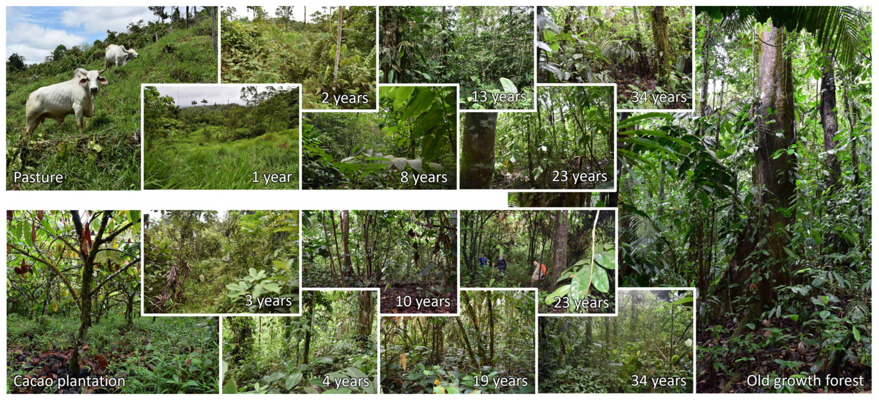
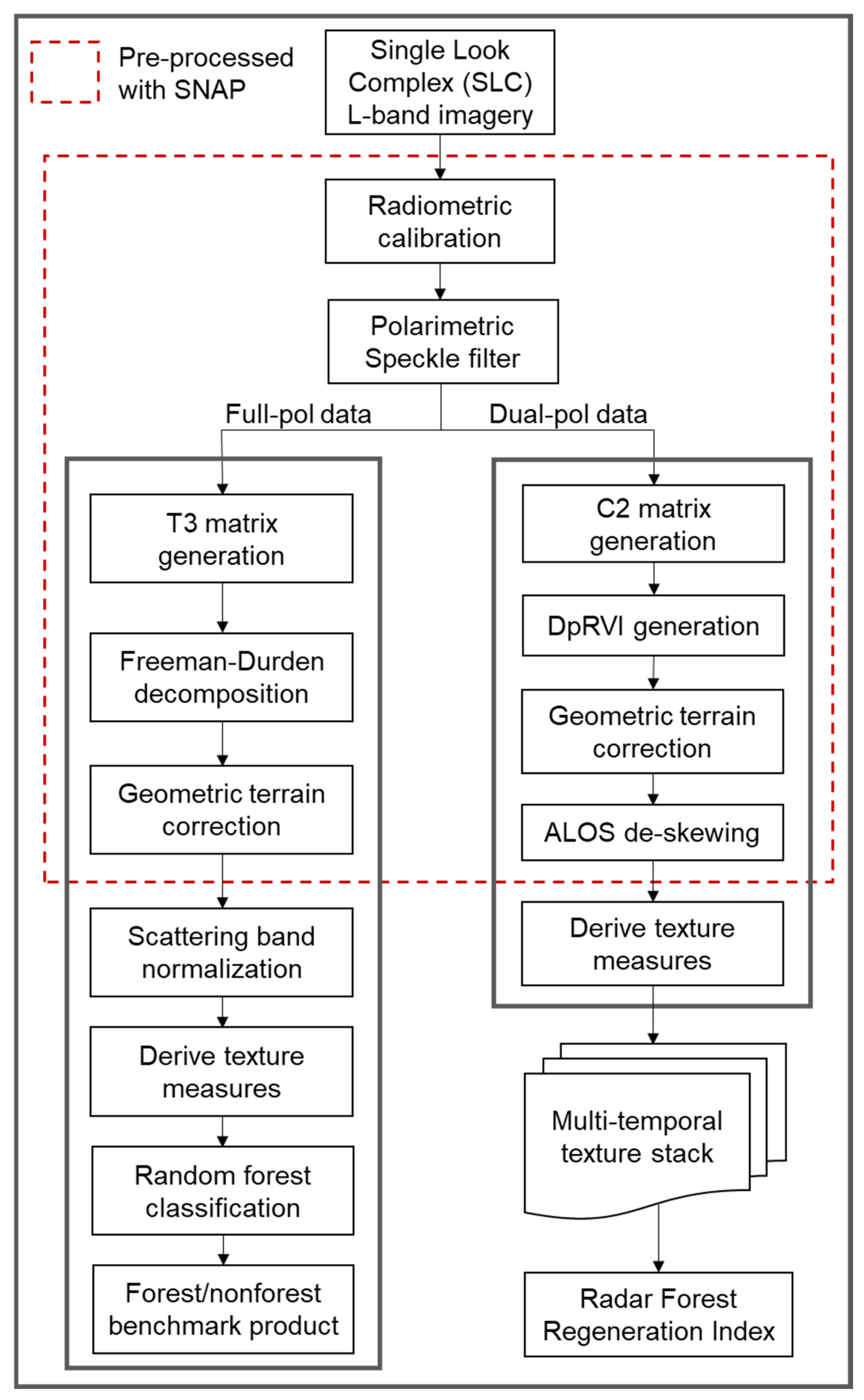
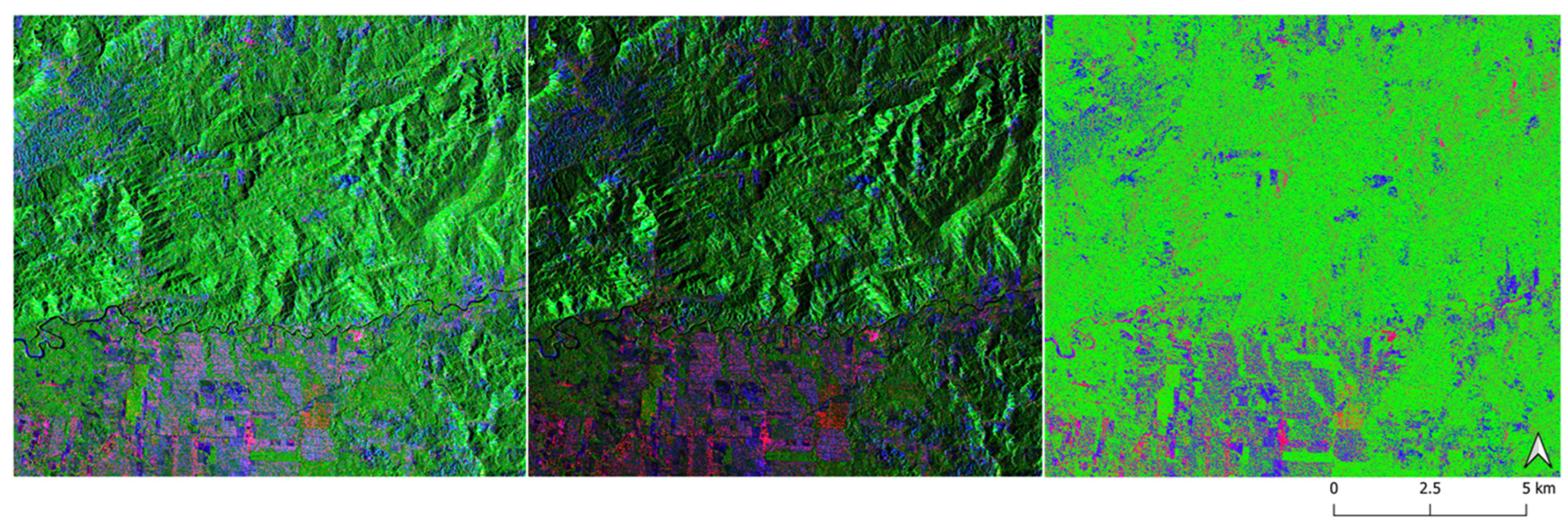
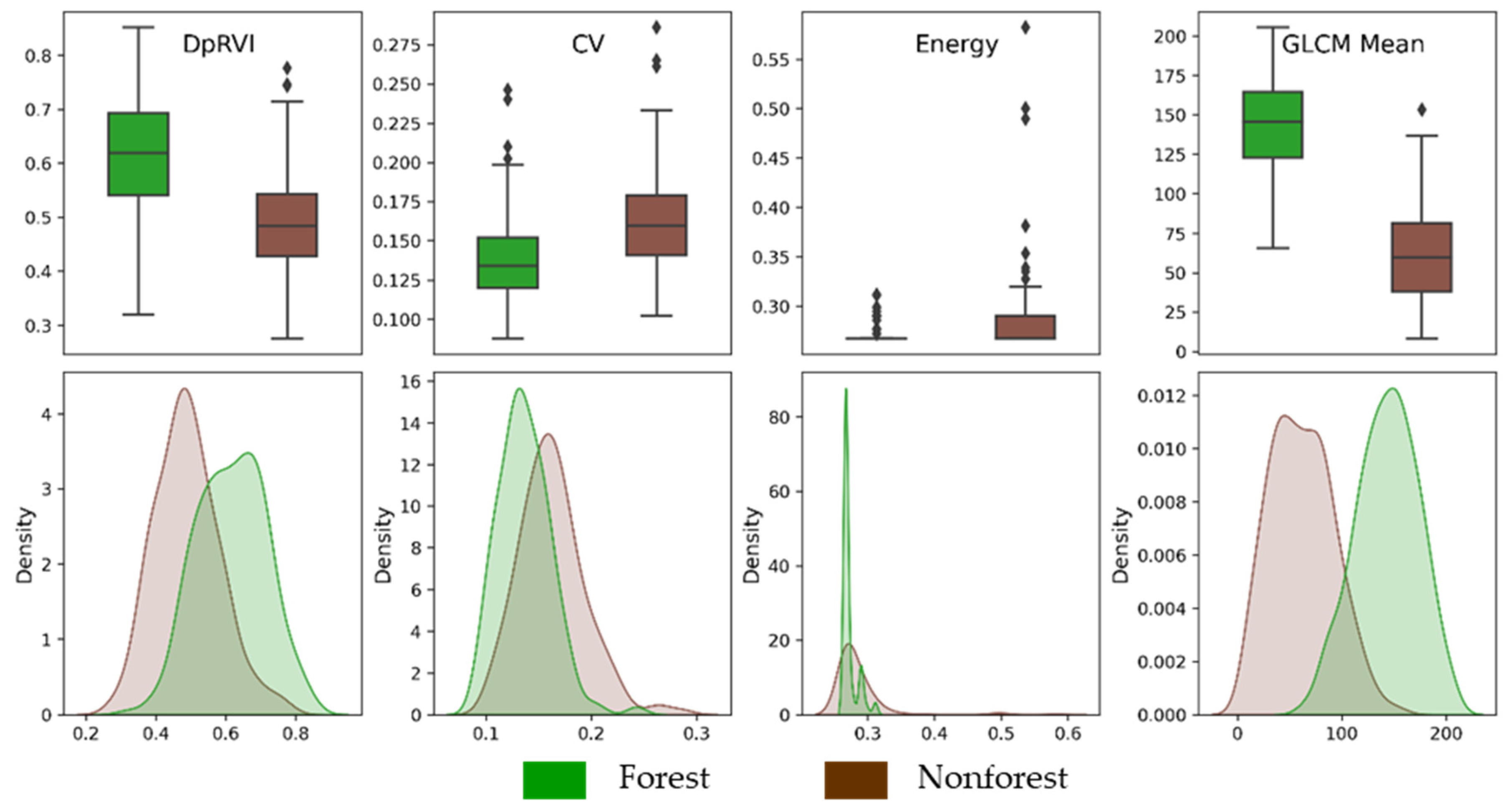
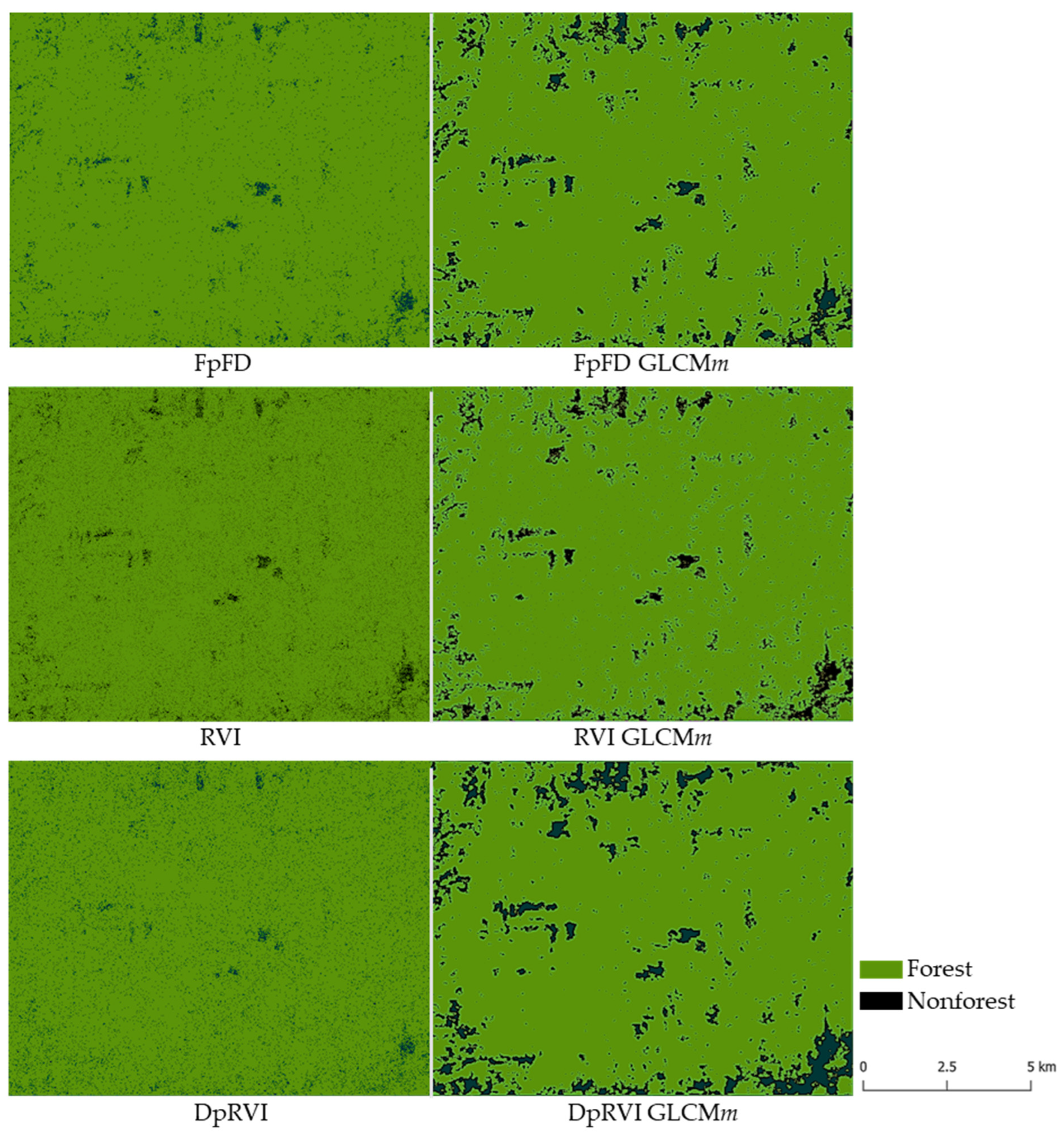
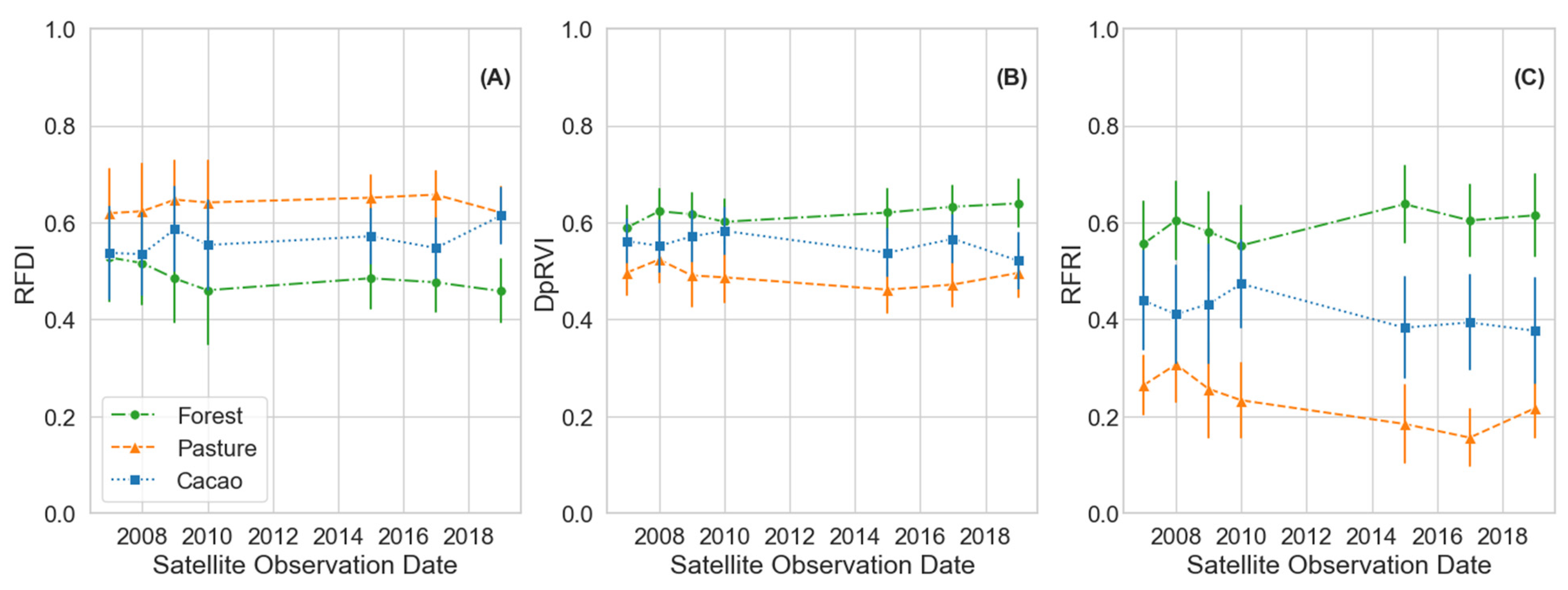
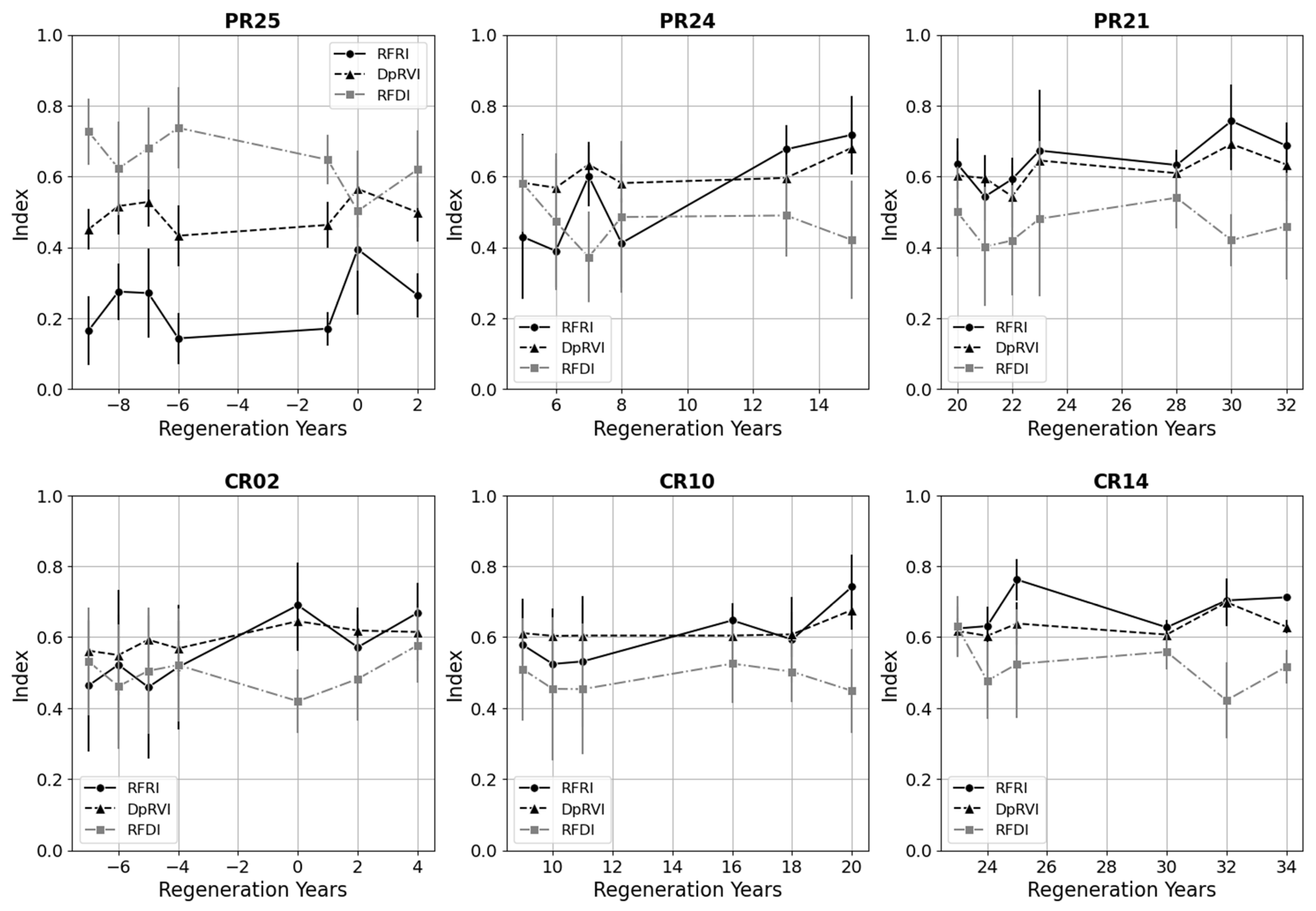
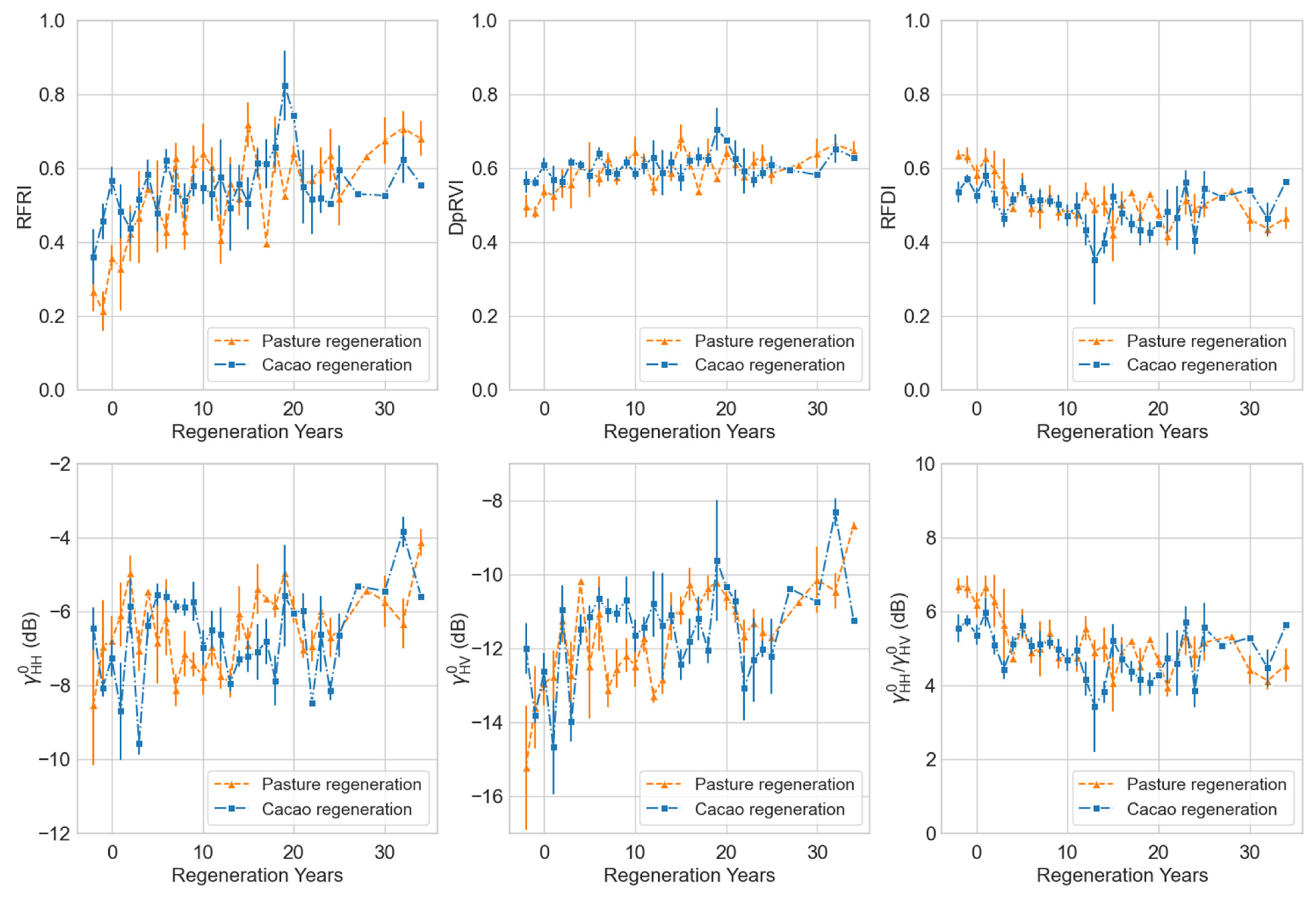

Disclaimer/Publisher’s Note: The statements, opinions and data contained in all publications are solely those of the individual author(s) and contributor(s) and not of MDPI and/or the editor(s). MDPI and/or the editor(s) disclaim responsibility for any injury to people or property resulting from any ideas, methods, instructions or products referred to in the content. |
© 2025 by the authors. Licensee MDPI, Basel, Switzerland. This article is an open access article distributed under the terms and conditions of the Creative Commons Attribution (CC BY) license (https://creativecommons.org/licenses/by/4.0/).