Ecological Network Construction and Optimization in the Southwest Alpine Canyon Area of China Based on Habitat Quality Assessment

Abstract

The Southwest Alpine Canyon Area (SACA) is a typical ecologically sensitive location in China; therefore, constructing and optimizing an ecological network for this area is essential to ensure the regional ecological security of its fragile ecosystems. This study employed the InVEST model to quantitatively assess the habitat quality of the SACA for the years 2000, 2010, and 2020. The ecological sources were determined based on the results of a habitat quality assessment and a Morphological Spatial Pattern Analysis (MSPA). Finally, ecological corridors, ecological pinch points, and ecological barrier points were identified using circuit theory. The results indicated that the SACA’s habitat quality was relatively good, but experienced slight degradation from 0.87 in 2000 to 0.84 in 2020. Anthropogenic activities have been identified as the primary contributor to habitat quality decline in the region. Geographically, the habitat quality is significantly poorer in the southeast and northwest of the SACA. A total of 319 ecological sources were identified, predominantly located in the southwest and northeast of the SACA, comprising 43.27% of the total area. Furthermore, 94 ecological corridors were delineated, covering an area of 74,015.61 km² and extending over 182.80 km in length in total. A total of 38 ecological pinch points and 39 ecological barrier points were distinguished, with a noticeable concentration in regions undergoing ecological degradation. Overall, while the ecological network structure in the SACA is complex and highly interconnected, it faces challenges relating to material cycling and ecological network circulation. Future ecological restoration and protection efforts should focus on areas along the border between the ecological maintenance area in southeastern Tibet (Region I) and the water conservation area in eastern Tibet–western Sichuan (Region II). Additionally, the establishment of ecological protection belts around potential ecological corridors is proposed to enhance ecosystem connectivity. These findings could provide a robust scientific foundation for territorial spatial planning, ecological preservation, and restoration in the SACA.

1. Introduction

Over the past few decades, socioeconomic development has intensified human pressures on global ecosystems [1,2], leading to widespread habitat fragmentation and loss. Alpine canyon areas are particularly vulnerable, being among the most sensitive regions to rapid shifts in socio-ecological dynamics [3]. Thus, mitigating the adverse impacts of anthropogenic activities on alpine canyon areas is of paramount importance. Ecological networks, representing the complex interactions between species and their environments, serve as essential frameworks for preserving biodiversity, sustaining ecosystem services, and enhancing ecological resilience [4,5]. Constructing and optimizing these networks is crucial for addressing the challenges associated with habitat fragmentation, human disturbances, and climate change, especially in alpine canyon regions.

The construction of ecological networks relies on diverse data sources, including environmental variables and interaction data. Advances in geographic information systems (GISs), remote sensing, graph theory, and landscape genetics have provided powerful tools for designing and optimizing ecological networks. Improvements in remote sensing technologies have enabled the use of high-resolution data, facilitating more accurate and comprehensive network models. The development of ecological networks generally involves extracting ecological sources, creating resistance surfaces, and identifying ecological corridors [6,7]. The optimization of ecological networks is achieved through spatial zoning and connectivity enhancements [8].

High-quality habitats, commonly referred to as core areas or ecological sources, are central to ecological networks. These areas provide the essential resources and conditions necessary for the survival and reproduction of species. Identifying and preserving ecological sources are critical for ensuring the effectiveness of these networks [9]. Opdam et al. [10] have emphasized that ecological sources must be substantial enough to support viable populations and demonstrate resilience to environmental changes. Early studies by Gurrutxaga et al. [11], Dong et al. [12], and Belote et al. [13] have identified protected areas and large forests as ecological sources; however, such a criterion is highly subjective. Habitat quality—defined as the capacity of the environment to provide conditions that are favorable for the persistence of individuals and populations [14]—is commonly used as a criterion for selecting ecological sources. Due to its simplicity and robustness, the InVEST model is considered to be one of the best-developed models for habitat quality assessments [15,16], and has been extensively utilized in various studies. For instance, Baral et al. [17] employed the InVEST model to investigate changes in biodiversity, while Liang et al. [18] used it to assess rhino habitat quality across regions in southern Zambia. Morphological Spatial Pattern Analysis (MSPA) has recently been introduced as a novel approach for the identification of ecological sources. The method employs a mathematical morphology approach to classify binary image pixels into seven mutually exclusive landscape types [19]. Given its minimal data requirements and user-friendly operation [20], the MSPA model has gained significant traction in research on the identification of ecological sources. However, relevant studies often rely on results from single-year analyses, which may lead to inaccurate ecological source identification. To date, few studies have examined long-term changes in habitat environmental quality [21]. To enhance the objectivity and reliability of ecological source selection, this research utilizes a three-year assessment of the Habitat Quality Index (HQI) alongside MSPA to identify ecological sources.

Ecological corridors are defined as linear habitats nested within a different matrix that connect two or more larger habitat blocks [22]. These corridors are linear features that link isolated habitats and are crucial for enhancing landscape connectivity. The resistance surface serves as the foundation for ecological corridor identification. Based on the constructed resistance surface, habitat patches with lower ecological resistance may connect to form ecological corridors [23]. Resistance coefficients are typically assigned based on land use types [24]. Once the resistance surface is constructed, ecological corridors can be identified based on the minimum cumulative resistance (MCR) model [25]. The MCR model calculates the minimal cumulative resistance distance between a source and a target to determine the best path for the migration and dispersal of species, thereby reducing external disturbances [26]. However, species migration paths can be diverse, and relying solely on the lowest-cost path can be overly simplistic [27]. Circuit theory, which simulates biological movement routes by quantifying multiple possible paths within the landscape, provides a more realistic representation of the movement of individual organisms [28]. Thus, in order to improve the spatial accuracy of ecological corridors, this research uses circuit theory to simulate and analyze the cumulative current value, thereby ascertaining the spatial location of ecological corridors. Moreover, the identification of ecological pinch points and barriers can further enhance the construction of a robust ecological network [29].

The construction and optimization of ecological networks have attracted increasing attention due to their significant potential for ecosystem management. Joel et al. identified seven large ecological networks in Uusimaa, Finland, using 59 high-quality layers of biotope and species distribution data [30]. Leoncini et al. analyzed ecological connectivity in the western Alps by applying electrical circuit theory to an expert-based resistance surface using the Circuitscape4.0.5 software [31]. Pineda-Zapata et al. identified high priority potential ecological corridors linking protected areas in Colombia [32]. Rosot et al. developed an ecological corridor network along Brazilian riparian zones to optimize landscape connectivity and species dispersal [33]. In the Zagros Mountains, Almasieh et al. systematically identified habitat patches and evaluated their connectivity patterns [34]. Field et al. employed least-cost path modeling in the Okanagan region to identify optimal wildlife movement routes [35]. Moreover, many existing studies have focused on constructing ecological networks based on specific target species [36]. While these approaches offer biological precision, they are typically suited for the conservation of specific species and require detailed ecological data, limiting their general applicability. In China, efforts to construct ecological networks have predominantly concentrated on urban landscape networks within the central and eastern regions [37,38]. For example, Xu et al. constructed the ecological network pattern of Suzhou to improve ecological quality [39], while Zeng et al. studied the ecological network of Zoigê County by identifying ecological sources based on the InVEST model [28]. However, the use of the InVEST model alone makes it difficult to capture spatial morphological attributes such as area and structural connectivity. Gu et al. directly used the remote sensing ecological index (RSEI) to map the ecological resistance surface and construct an ecological network in the Qinghai–Tibet area, although they did not identify ecological sources within the study area [40].

The Southwest Alpine Canyon Area (SACA), located in the Hengduan Mountains of Southwest China, is known for its towering peaks and steep valleys [41]. Approximately 65% of this region consists of mountains exceeding 3500 m in elevation. Due to its unique topography and complex climate, the SACA is widely recognized as one of China’s most ecologically fragile regions [42]. It not only boasts rich biodiversity and complex ecosystems, but also serves as a crucial habitat for numerous rare and endangered species. Moreover, with many significant rivers, such as the Mekong River, Salween River, and Jinsha River, originating here, the SACA is a vital water conservation zone that plays an irreplaceable role in securing water supplies for downstream regions. Existing research on the SACA has mainly focused on the soil erosion process [43], the driving mechanisms of vegetation change [44], vegetation restoration techniques [45], and climate change [46]. As one of the most complex terrains and biologically diverse ecological transition zones in China, the characteristics of the evolution of habitat quality in the SACA remain unclear; furthermore, an ecological network assessment method that matches the unique geographical characteristics of this area has not been previously established. Therefore, our study develops a generalizable framework for ecological network construction and optimization in the SACA that integrates habitat quality assessment (InVEST), Morphological Spatial Pattern Analysis (MSPA), the Least Cumulative Resistance (LCR) model, and circuit theory. This is the first implementation of such an integrated methodology in the SACA. This application not only addresses the gap in ecological network research within alpine canyon ecosystems, but also offers a replicable technical template for ecosystem management in comparable geomorphological regions worldwide.

Consequently, the main objectives of this study are as follows: (1) to quantitatively evaluate the habitat quality of the SACA using the InVEST model; (2) to identify ecological sources, corridors, pinch points, and barrier points based on multi-source geographic data, thereby constructing a robust ecological network; and (3) to propose optimization measures for the ecological network to enhance landscape connectivity and ecosystem resilience in the SACA. This study aims to provide a scientific basis for ecological restoration and conservation initiatives in the SACA.

2. Materials and Methods

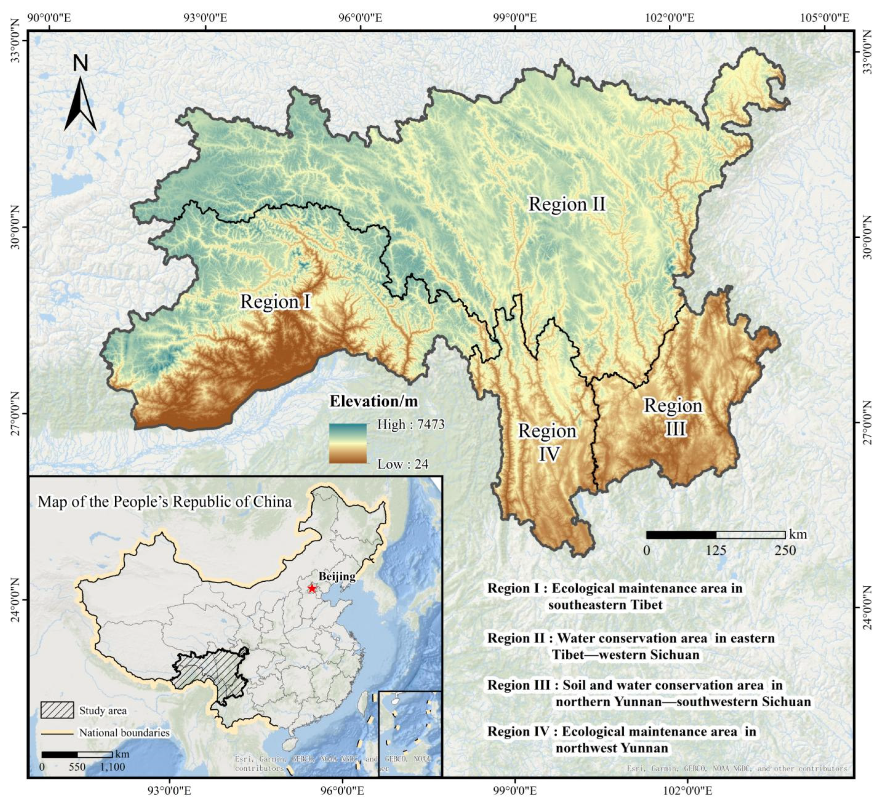
2.1. Study Area

The SACA is located at the intersection of Sichuan Province, Yunnan Province, and the Tibet Autonomous Region in China (Figure 1), covering an area of approximately 614,000 km². It is geographically situated between 24°58′7.47″~32°51′24.93″N and 91°23′48.24″~104°13′43.55″E. Elevations in this area vary from 24 m to 7473 m, resulting in a steep topography. The geomorphology is predominantly characterized by mountainous terrain and high plateaus, featuring seven parallel mountain ranges and six major rivers, commonly referred to as the “Seven Ranges and Six Rivers”. The SACA exhibits a distinct vertical climate zonation, with the average annual rainfall varying between 300 and 2300 mm and temperatures ranging from −3 to +22 °C. The rainfall distribution increases from north to south and from west to east. This complex and heterogeneous climate, along with the distinctive natural geography, has fostered a rich diversity of vegetation types. The predominant land use types in this area are woodlands and grasslands, accounting for 46% and 28% of the total area, respectively. Additionally, the SACA serves as a refuge for numerous uncommon and endangered species, and is recognized as a vital water source for the nation.

According to the “Soil and Water Conservation Regionalization Map of China” created by the Ministry of Water Resources of the People’s Republic of China [47], the SACA can be divided into four distinct areas: the ecological maintenance area in southeastern Tibet (Region I), the water conservation area in eastern Tibet–western Sichuan (Region II), the soil and water conservation area in northern Yunnan–southwestern Sichuan (Region III), and the ecological maintenance area in northwest Yunnan (Region IV).

2.2. Data Sources

This study utilized multiple geospatial datasets (

Table 1. Data sources and pre-processing.

Data Type	Source	Website	Type	Original Spatial Resolution	Time
Land use	the GlobeLand30 V2020 series provided by the Ministry of Natural Resources	https://www.ngcc.cn/xwzx/ywcg/202401/t20240103_1270.html (accessed on 28 February 2024)	Raster	30m	2000, 2010, 2020
NDVI	the 2022 MODIS image MOD13Q1 product from NASA	https://modis.gsfc.nasa.gov/ (accessed on 17 December 2023)	Raster	250m	2022
DEM	GDEMV3 provided by the Geospatial Data Cloud Platform	https://www.gscloud.cn/ (accessed on 5 December 2023)	Raster	30m	2022
Nature reserves	the China Nature Reserve Specimen Resource Sharing Platform	http://bhq.papc.cn/specimen.html (accessed on 29 April 2020)	Vector	-	2022
Road	the OpenStreetMap platform	https://openmaptiles.org/ (accessed on 27 January 2024)	Vector	-	2022

), including data on roads, nature reserves, the normalized difference vegetation index (NDVI), a digital elevation model (DEM), and land uses. The land use data were classified into six categories: farmland, woodland, grassland, water, artificial surfaces, and bare land. The accuracy of land use data provided by GlobeLand30 exceeds 80%, making it a widely used resource in many relevant studies [48,49,50,51,52,53,54]. Annual NDVI values were synthesized using the maximum value composite (MVC) method. Slope and elevation data were derived from the DEM. The nature reserve data, in Keyhole Markup Language Zipped (KMZ) format, were vectorized using ArcGIS 10.8. Railway and trunk road data were obtained from OpenStreetMap. All datasets were projected to WGS 1984 UTM Zone 47N and resampled to a spatial resolution of 250 m.

The spatial resolution was unified to 250 m for the following reasons: (1) to meet GuidosToolbox’s technical limitations for MSPA (maximum raster size of 10,000 × 10,000 pixels [55], approximately 95.4 MB uncompressed for 8-bit single-band data); (2) to optimize computational efficiency for InVEST model simulations without compromising the integrity of landscape pattern representation; and (3) to ensure spatial alignment among datasets for ecological resistance surface construction.

2.3. Methods

Figure 2 presents the framework of this study, which consists of seven steps for the construction and optimization of the ecological network. The first step is data collection. The second step is habitat quality assessment. The third step is to extract ecological sources by overlaying the habitat quality and MSPA results. Subsequently, an ecological resistance surface for the SACA is developed, incorporating seven resistance factors. In the fifth and sixth steps, key elements of the ecological network, such as ecological sources, corridors, pinch points, and barrier points, are identified. Finally, the seventh step entails the optimization of the ecological network and the formulation of specific recommendations for ecosystem management, based on the findings from the previous steps.

2.3.1. Assessment of Habitat Quality

The HQI serves as a key measure for evaluating how well various forms of land usage adapt to habitats, as well as indicating an ecosystem’s resilience to various threats. The SACA’s habitat quality was assessed using the InVEST model’s habitat quality module, which involved assessing the current state and degradation level of the ecosystem in terms of both its intrinsic characteristics and external threats. Numerous related studies have employed the high-precision outputs from the InVEST model [56,57,58], demonstrating its reliability and value as a reference tool in assessing key ecosystem services such as habitat quality. This study extracted habitat threat source data based on raster data of land use types in order to quantitatively assess the detrimental effects of threat sources on habitats. The formula is given below:

$$Q_{xj}=H_j(1-{\displaystyle \frac{D_{xj}^2}{D_{xj}^2+K^2}})$$

(1)

where Q_xj is the habitat quality index of grid cell x for land use and cover type j; H_j is the habitat appropriateness of land use and cover type j; D_xj is the degradation degree of the habitat of grid cell x for land use and cover type j; and K is the half-saturation constant, with a default value of 0.5. The following formula is used to determine D_xj:

$$D_{xj}=\sum _{r=1}^R\sum _{y=1}^{Y_r}\left({\displaystyle \frac{W_r}{{\sum }_{r=1}^R{W}_r}}\right)r_y\cdot i_{rxy}{\cdot \beta }_x{\cdot S}_{jr}$$

(2)

$$i_{rxy}=1-\left({\displaystyle \frac{d_{xy}}{d_{rmax}}}\right)(if linear)$$

(3)

$$i_{rxy}=\mathit{exp}({\displaystyle \frac{-2.99d_{xy}}{d_{rmax}}}) (if exponential)$$

(4)

where R denotes the number of stressors; y is all of the grid cells of stressor r; Y_r is the number of rasters of stressor r; W_r is the weight of stressor r; r_y is the value of stressor r of raster y; i_rxy is the stress level of stressor r_y from raster y on raster x; β_x is the accessibility of the stressor to raster x; S_jr is the sensitivity degree of habitat type j to stressor r, with the value range [0, 1]; d_xy is the distance in linear terms between raster x and raster y; and d_{r max} is the greatest distance under stress of stressor r.

Considering the unique geographical characteristics of the SACA, and based on the relevant literature [59,60,61,62,63] and InVEST modeling guidelines [15], this study took bare land, artificial surfaces, and farmland as threat factors (

Table 2. Habitat threat sources and their maximum impact distances, weights, and attenuation types.

Source of Threat	Maximum Distance/km	Weight	Decay
Farmland	5	0.6	Linear
Artificial surface	9	0.9	Exponential
Bare land	4	0.3	Linear

), which were assigned corresponding weights. Artificial surfaces are typically areas with the most intensive human activity and exert significant disturbance effects on ecosystems, leading to high ecological vulnerability. Therefore, a weight of 0.9 was assigned to reflect their considerable impact on habitat quality. Farmland is frequently subject to anthropogenic disturbances due to agricultural activities, such as mechanized operations and the application of fertilizers and pesticides, and was thus assigned a weight of 0.6. Bare land, characterized by low vegetation cover and weak ecosystem functioning, remains naturally exposed for long periods. Its relatively minor influence on surrounding environments is reflected by its lower weight of 0.3. Based on the actual conditions, the maximum impact distance and corresponding weights for each threat factor were determined, along with habitat suitability and the sensitivity of different habitat types to these threats (

Table 3. Parameters of habitats’ appropriateness and sensitivity to threat sources for different land uses.

Land Use Type	Habitat Appropriateness	Source of Threat
		Farmland	Artificial Surface	Bare Land
Farmland	0.4	0	0.5	0.3
Grassland	0.8	0.5	0.6	0.2
Bare land	0.1	0	0.1	0
Woodland	1	0.7	0.8	0.4
Water	0.9	0.6	0.7	0.3
Artificial surface	0	0	0	0

).

Finally, the results were categorized into five ranges in ArcGIS 10.8 using the natural breakpoints approach. The Natural Breaks (Jenks) method is a classification technique that identifies natural groupings by minimizing the variance within classes while maximizing the variance between classes.

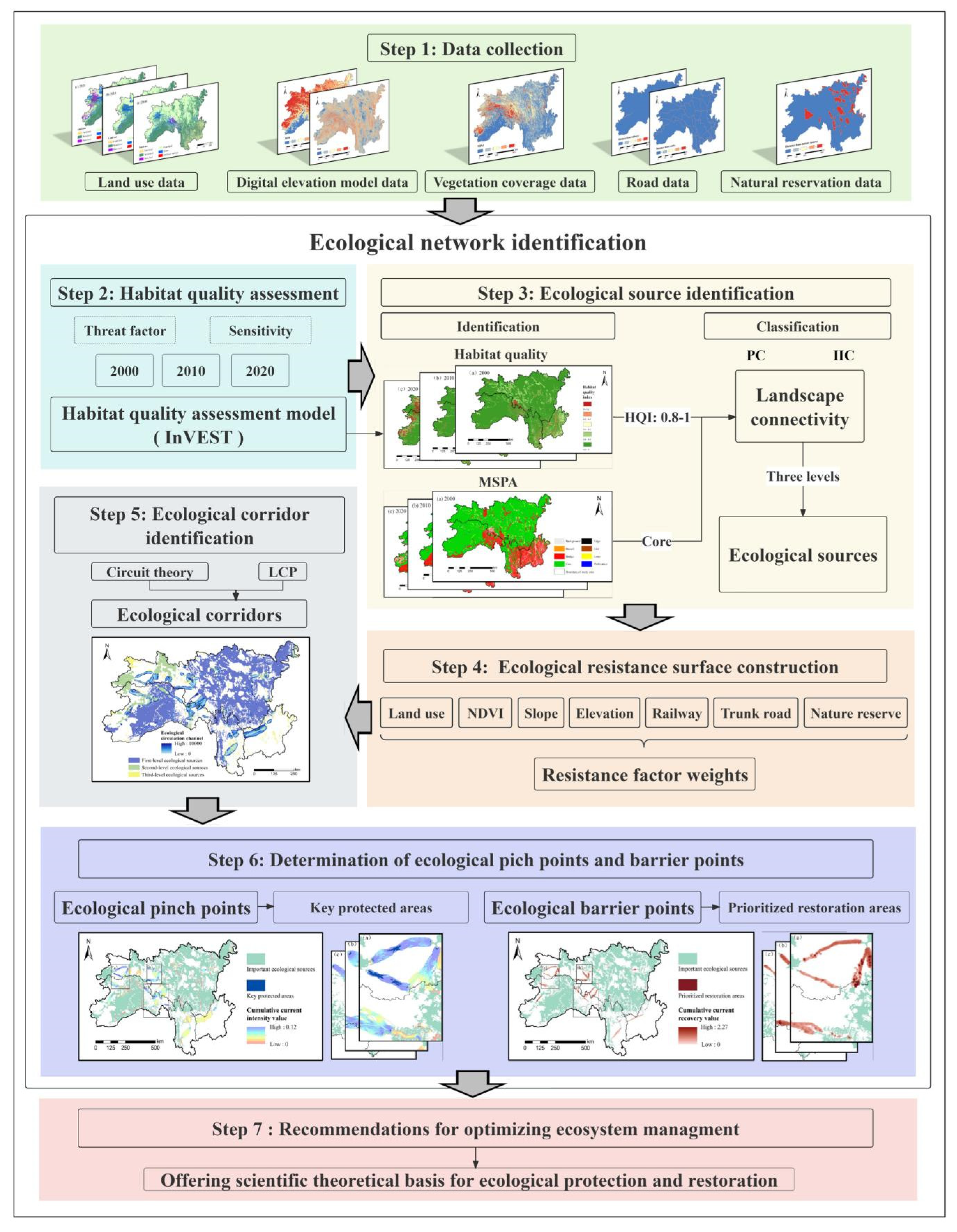
2.3.2. Construction of Ecological Network

• Identification of ecological source

MSPA is a mathematical morphology-based technique that classifies binary image pixels into seven exclusive landscape types: core, branch, bridge, edge, loop, islet, and perforation [64]. The “core” typically refers to large natural patches, such as forest reserves and habitats for animals. In the SACA, three land types known for their high biodiversity—namely, woodland, water, and grassland—were designated as foreground, while all other land types that do not contribute significantly to biodiversity were classified as background [65]. This classification emphasizes the importance of maintaining and conserving these high-biodiversity areas for ecological health. The MSPA was conducted using the Guidos Toolkit 3.0 software [66].

Ecological sources are crucial natural regions that provide essential ecosystem services and are often characterized by high habitat quality and strong landscape interconnectedness. In this study, areas with an HQI ranging from 0.8 to 1.0 and an MSPA classification of core were considered to be ecological sources.

Landscape interconnectivity serves as a critical indicator of the interaction degree between ecological patches within a region, which is essential for the preservation of biodiversity and ecological services [67,68]. Through an analysis of the Integral Index of Connectivity (IIC) and Possible Connectivity (PC), the importance rank and conservation order of ecological sources can be better determined [69,70]. In this context, setting reasonable distance thresholds is essential for accurate assessment [71]. In this study, the IIC and PC were computed using the Conefor 2.6 software, with the connection probability set at 0.5 and the connectivity threshold set at 3000 m. The calculation formula is as follows:

$$PC={\displaystyle \frac{{\sum }_{i=1}^n{\sum }_{j=1}^n{a}_i\cdot a_j\cdot p_{ij}^{*}}{A_L^2}}$$

(5)

$$IIC={\displaystyle \frac{{\sum }_{i=1}^n{\sum }_{j=1}^n\left[\right(a_i\cdot a_j)/(1+n{l}_{ij} )]}{A_L^2}}$$

(6)

where n represents the total quantity of patches, a_i and a_j are the areas of patch i and patch j, A_L represents the whole area of the landscape, P_ij^* represents the maximum possibility of diffusion between patch i and patch j, and nl_ij represents the number of connections in the shortest paths between patch i and patch j.

2.

Construction of ecological resistance surface

The ecological resistance surface is used to determine the migration routes of animals across areas with varying degrees of resistance. In this study, the Least Cumulative Resistance (LCR) model was employed to calculate the cumulative energy consumption of ecological flows, thus identifying the path with the least energy consumption and estimating the spatial resistance to organism movement. The SACA, distinguished by its rich biodiversity and numerous endangered species, encompasses several natural reserves. Additionally, the recent construction of the Sichuan–Tibet Railway has further impacted the environment in this region. Therefore, land use types, slope, elevation, NDVI, distance to natural reserves, distance to railways, and distance to trunk roads were selected as resistance factors to construct the ecological resistance surface. The weights of these factors were determined based on the relevant literature [72,73,74,75,76] (

Table 4. Resistance factors and their weights.

Resistance Factor	Resistance Value					Weights
	1	2	3	4	5
Land use type	Woodland	Water and grassland	Farmland	Bare land	Artificial surface	0.45
NDVI	≥0.84	0.70–0.84	0.51–0.70	0.26–0.51	≤0.26	0.05
Slope/(°)	≤13.25	13.25–23.44	23.44–32.96	32.96–43.15	≥43.15	0.09
Elevation/m	≤1776	1776–2864	2864–3792	3792–4568	≥4568	0.10
Distance from a nature reserve/km	≥2.00	1.00–2.00	0.50–1.00	0.30–0.50	≤0.30	0.07
Distance from a railway/km	≥2.00	1.50–2.00	1.00–1.50	0.50–1.00	≤0.50	0.13
Distance from a trunk road/km	≥1.20	0.80–1.20	0.60–0.80	0.30–0.60	≤0.30	0.11

).

By spatially superimposing the ecological resistance factors of each level indicator, a comprehensive ecological resistance surface for the SACA was developed using ArcGIS 10.8. The equation is shown below:

$$R_i=\sum _{i=1}^n{w}_i·f_j\left(i\right)$$

(7)

where R_i is the resistance value of the i-th raster cell on the ecological resistance surface; n is the total number of resistance-influencing factors considered; w_j is the weight assigned to the j-th factor, reflecting its relative importance in impeding species movement; and f_j(i) is the standardized resistance contribution of the j-th factor for cell i.

3.

Identification of ecological corridors

Ecological corridors form low-resistance paths connecting ecological sources for the migration of animals, ensuring the smooth flow of elements [77,78]. Utilizing circuit theory [7], this study used the Linkage Mapper module to input first- and second-level ecological sources and resistance surfaces to locate ecological corridors and potential corridors. This method can depict the optimal movement routes and alternative paths across heterogeneous landscapes, and subsequently obtain ecological corridors and their lengths and resistance values.

4.

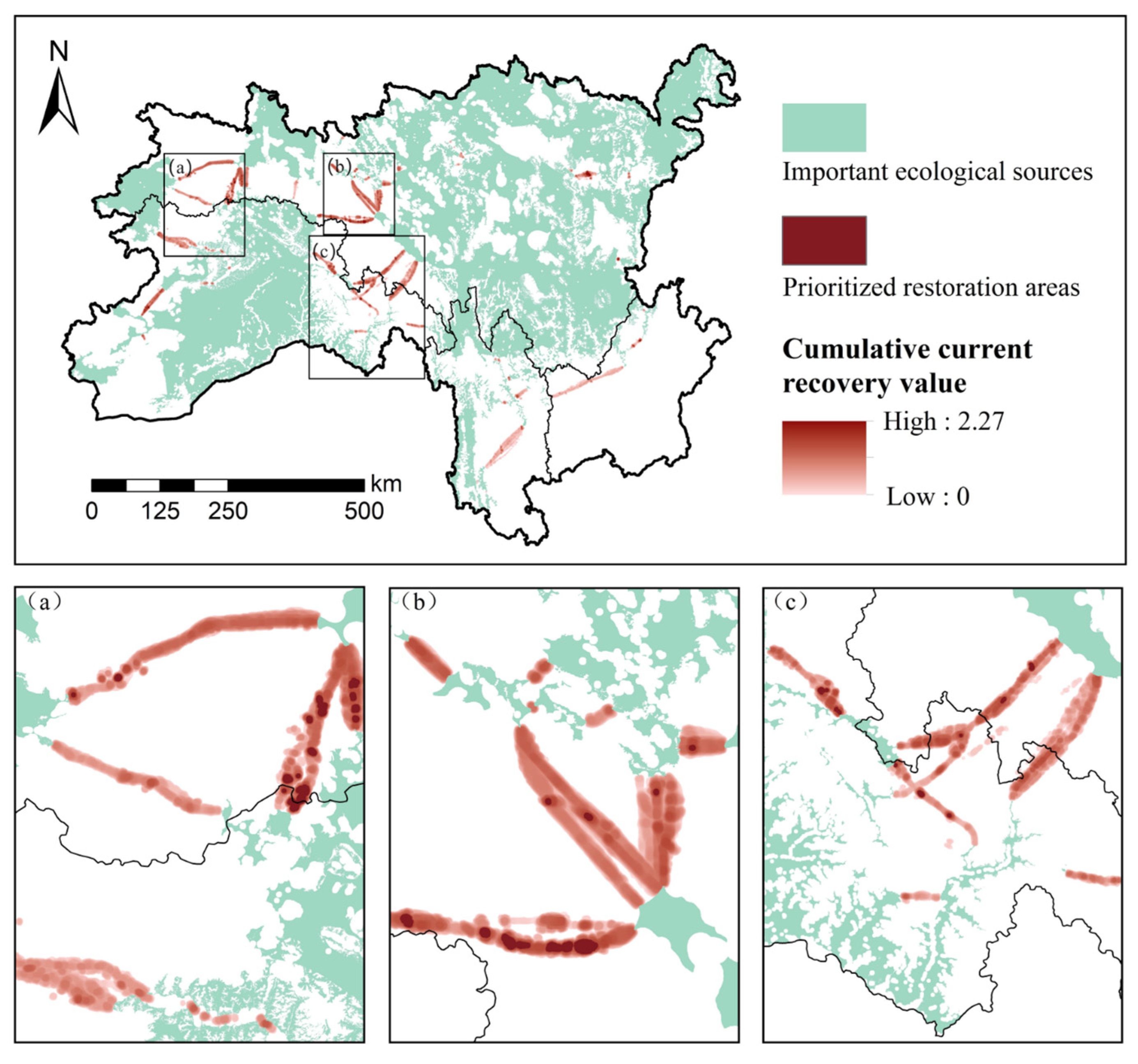
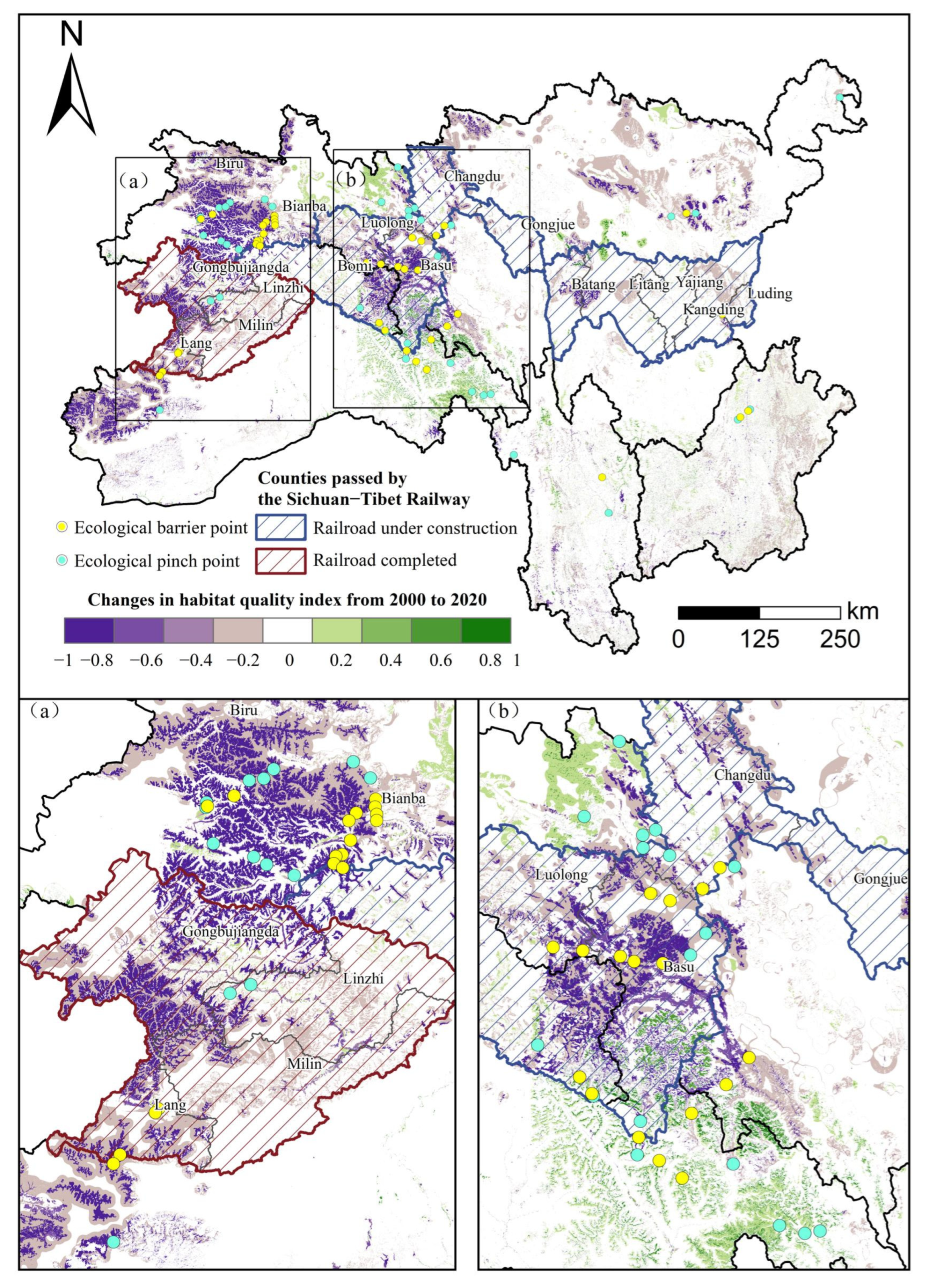
Determination of ecological pinch points and barrier points

Landscape features that are critical to the interconnectivity of ecological sources are referred to as ecological pinch points. These areas are necessary for animal activities, as they not only enhance habitat accessibility but also reduce ecological risk across the entire region. From the perspective of circuit theory, ecological pinch points hold particular significance due to their high current density and irreplaceable characteristics. In this study, ecological pinch points were effectively identified using the Pinch point Mapper tool within the Circuitscape software, along with iterative calculations employing an “all to one” model.

Conversely, ecological barrier points are locations where species encounter difficulties migrating between ecological sources. Eliminating these barriers can significantly improve the connectivity of ecological sources. The locations of ecological barrier points can be accurately determined by establishing a specific search radius based on circuit theory. The “Maximum” setting of the Circuitscape software’s Barrier Mapper tool was chosen for this study’s iterative computations to locate ecological barriers [79].

3. Results

3.1. Spatial and Temporal Characteristics of Habitat Quality

In the SACA, the HQI was 0.87 in 2000, 0.86 in 2010, and 0.84 in 2020. Despite the generally high habitat quality, a noticeable downward trend was evident. The extent of high-quality habitat (HQI 0.8–1.0) contracted markedly, while areas classified as low-quality habitat (HQI 0.0–0.2) expanded significantly, particularly over the period of 2010–2020 (Figure 3). To better understand the geographical distribution of habitat quality across the SACA, this study classified the HQI into five categories. Between 2000 and 2020, high-quality habitat areas declined by 12.51%, whereas low-quality habitat areas increased by 4.51% (Figure 4).

Spatially, the most significant declines in habitat quality during the 2000–2020 period were observed in the ecological maintenance area in southeastern Tibet (Region I) and the water conservation area in eastern Tibet–western Sichuan (Region II), where the HQI decreased from 0.90 to 0.86 and 0.86 to 0.82, respectively. Especially in the 2010–2020 period, extensive areas of low habitat quality appeared in these two areas. Moreover, the habitat quality of Region II exhibited considerable fragmentation, with habitat patches of varying quality interspersed, creating a complex mosaic pattern. In contrast, the habitat quality in northern Yunnan–southwestern Sichuan (Region III) and the ecological maintenance area in northwest Yunnan (Region IV) remained relatively stable during 2000–2020. The average HQI in Region IV was as high as 0.90, whereas Region III maintained a relatively lower level of approximately 0.82.

3.2. Identification and Distribution of Ecological Sources

3.2.1. Analysis of Morphological Spatial Patterns

Figure 5 presents the results of the MSPA for the SACA. A comparison with the habitat quality assessment revealed that areas with higher habitat quality were largely consistent with core areas, exhibiting a similar spatial distribution of landscape elements across the three time periods. However, from 2000 to 2020, the total area of core patches decreased by 13.64%. This reduction primarily occurred in the transitional zone between Region I and Region II, where core areas were predominantly converted into bridge and background types. The area of bridge elements increased by 4.19% during this period, primarily along the boundaries between core and background areas. By 2020, bridge elements accounted for 24.62% of the total study area. Other landscape types showed relatively low proportions and scattered distributions.

3.2.2. Spatial Distribution of Ecological Sources

Based on the habitat quality assessment and MSPA results, a threshold of 10 km² was determined, after multiple trials, to be the most suitable criterion, ensuring that the identified ecological sources correspond to realistically protectable areas. Cores with an HQI of 0.8–1 and an area larger than 10 km² across all three periods were classified as ecological sources. A total of 319 ecological sources covering 264,183.83 km² were identified, thus accounting for 89.90% of the total core area and 43.27% of the study area. As shown in Figure 6, woodland was the dominant component of these ecological sources, covering 147,896.98 km² (55.76% of the total ecological source area), followed by grassland, which constituted 35.63%. These findings highlight the critical role of woodland and grassland in maintaining ecological security in the SACA. Meanwhile, areas with a PC value ≥ 1 were designated as first-level ecological sources, those with values between 0.1 and 1 as second-level sources, and the remaining as third-level sources. Finally, there were 17 first-level, 28 second-level, and 273 third-level ecological sources, accounting for 34.66%, 5.68%, and 2.69% of the SACA, respectively. According to Figure 7, first-level and second-level ecological sources were mostly concentrated in Region I and Region II. In Region I, the sources were primarily concentrated in the central area, with fewer sources on the eastern and western sides. Region II contained the highest density of ecological sources within the entire study area. In Region III, the low habitat quality resulted in fewer and smaller ecological sources. Region IV presented a narrow, north–south-oriented band of ecological sources along its western edge, covering a small area.

3.3. Identification and Distribution of Ecological Corridors

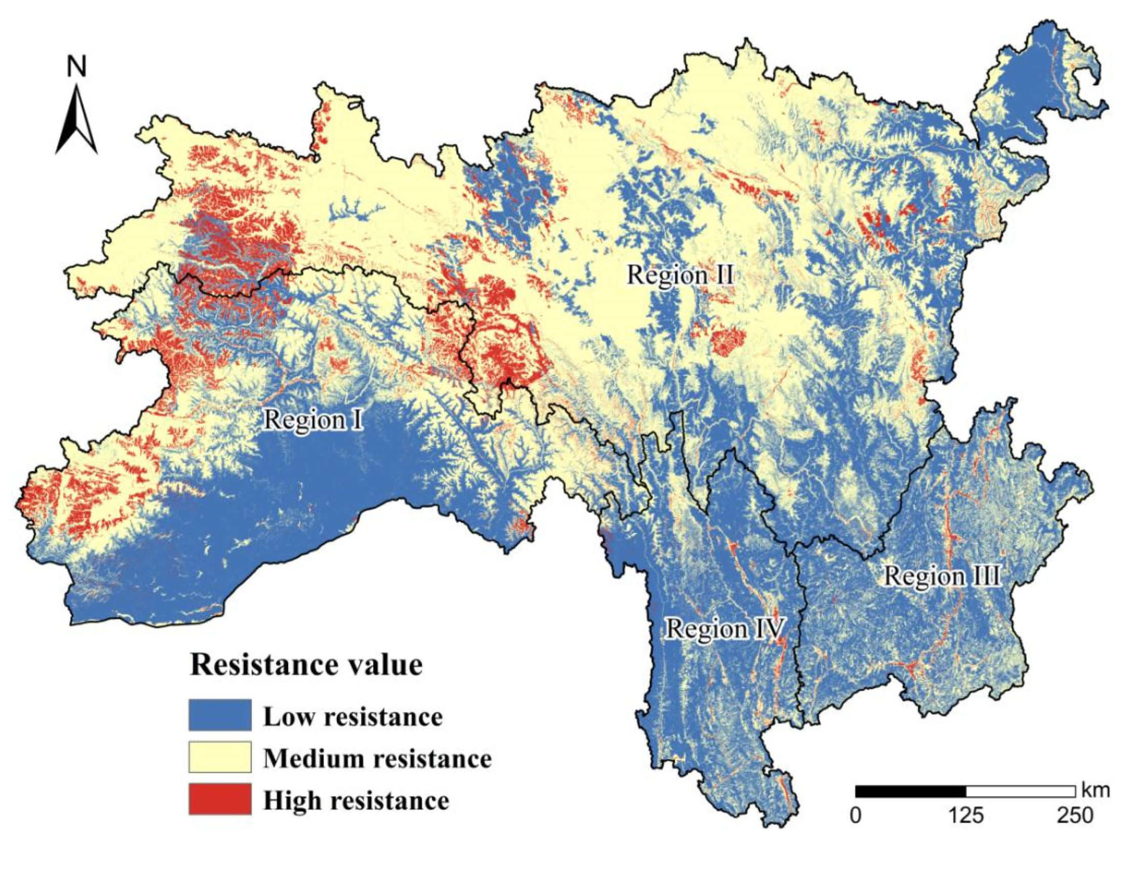
3.3.1. Analysis of Ecological Resistance Surface

The ecological resistance surface was constructed by assigning weight coefficients to each resistance factor based on its corresponding resistance value (Figure 8). To analyze the spatial distribution of the ecological resistance surface in the SACA, this research employed the Natural Breaks method in ArcGIS 10.8 to categorize the ecological resistance into three levels: low, medium, and high resistance.

The results revealed significant regional variations in the ecological resistance values. The northwestern part of the study area predominantly consisted of medium-resistance areas, while the southeastern part was primarily classified as low resistance. Low-resistance areas were mainly located at low elevations and characterized by high vegetation cover and good habitat quality, notably in Region III, Region IV, and Region I. In contrast, medium and high resistance were mostly observed in areas with rugged terrain and poor habitat quality, thus impeding animal migration.

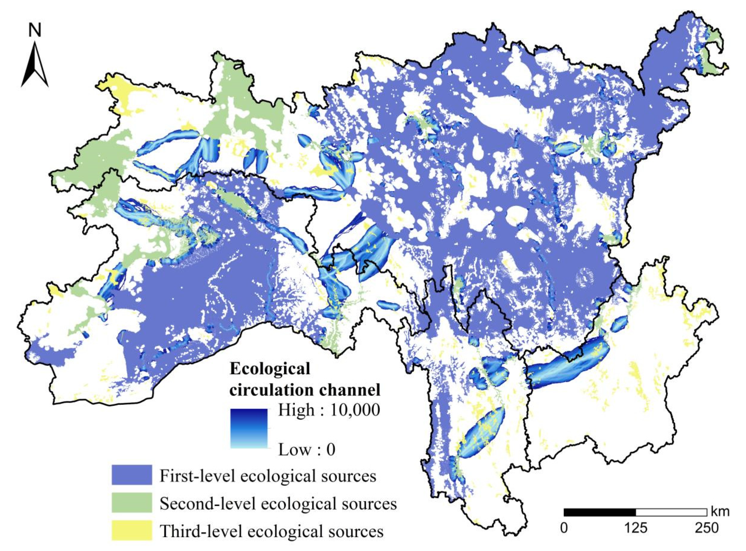
3.3.2. Spatial Distribution of Ecological Corridors

Based on the first-level and second-level ecological sources in the SACA, this study employed the ecological resistance surface (Figure 8) and circuit theory to generate 94 ecological corridors, encompassing a total area of 74,015.61 km² and a cumulative length of 182.80 km. Longer ecological corridors with higher levels of ecological resistance are more vulnerable to fragmentation. Consequently, the ecological corridors were categorized into two levels, based on their lengths and ecological resistance values. Among these, 16 first-level ecological corridors were shorter and exhibited lower resistance, while 78 second-level corridors were longer and more resistant. The primary components of these ecological corridors were woodland and grassland, covering areas of 37,815.30 km² and 2238.80 km², respectively, accounting for 51.09% and 30.45% of the entire corridor region (Figure 6).

As depicted in Figure 7, the ecological corridors in the SACA primarily serve to connect first-level ecological sources and exhibit an uneven spatial distribution. These corridors were mostly centered at the junction of Region I and Region II, where the level of interaction among ecological sources is high. In contrast, the southwestern region of the SACA possessed more favorable ecological conditions and higher habitat patch integrity, resulting in a reduced number of ecological corridors functioning as connectors in this area. In the northeastern part of the SACA, although there were numerous ecological sources, they were relatively scattered. Many of the nearby ecological sources were linked by short first-level ecological corridors, contributing to a more complex structure of the ecological network. Furthermore, most sources were connected by only one corridor, rendering them vulnerable to disturbances and reducing overall network connectivity.

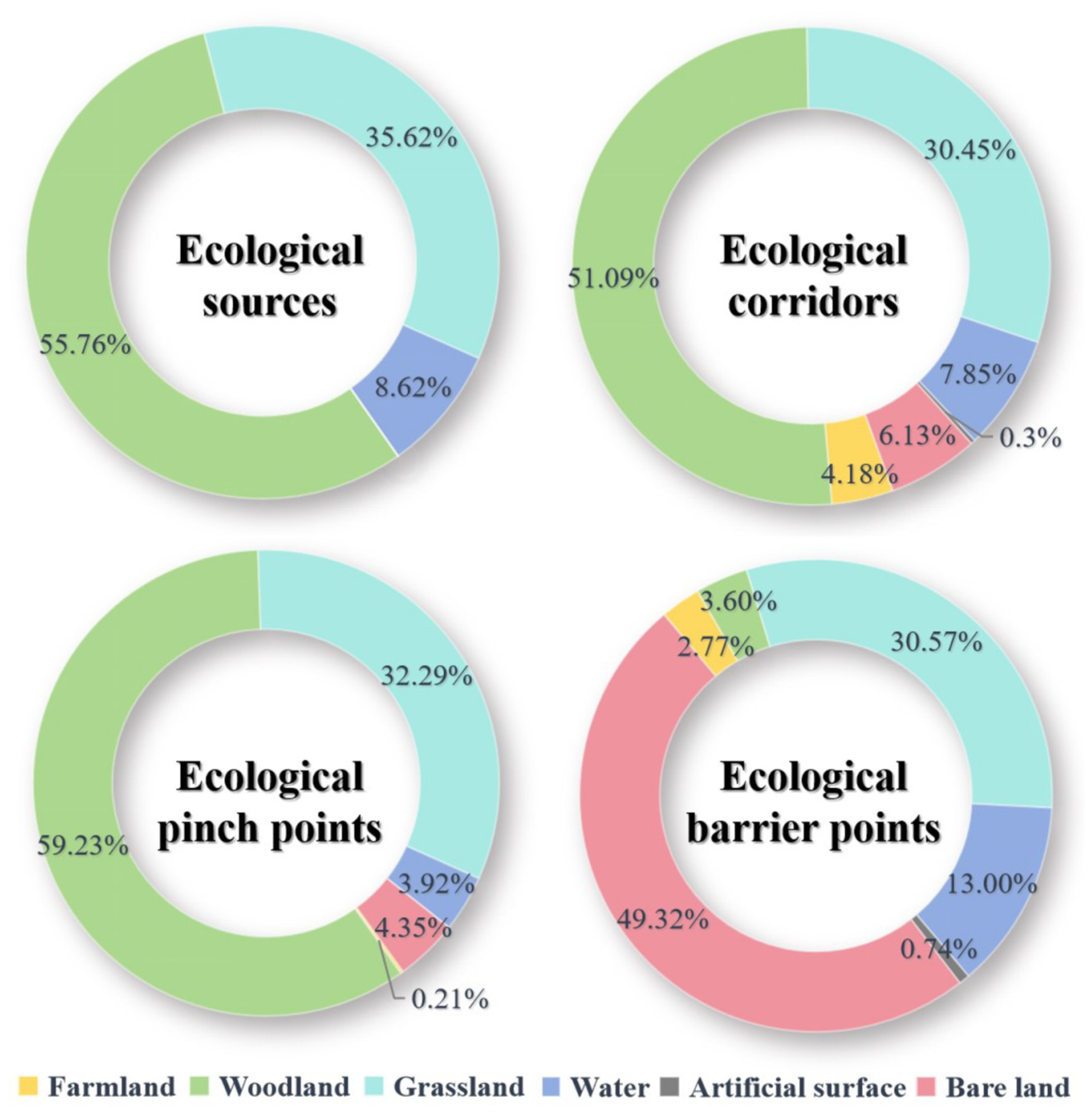
3.4. Spatial Characteristics of Critical Ecological Nodes

Ecological pinch points along the corridors primarily emerge in areas traversable by wildlife but are surrounded by landscapes of high resistance. These areas are highly susceptible to fragmentation and, thus, represent priority sites for conservation efforts. In the SACA, 38 pinch points covering a total area of 538.98 km² were found (Figure 9). The majority of these ecological pinch points were located within the second-level ecological corridors at the junction of Region I and Region II. The predominant land use types in these areas were woodland and grassland, which constitute 59.23% and 32.29% of the overall key protected area, respectively (Figure 6). Incorporating these ecological pinch points into the ecological network is essential for enhancing the connectivity of ecological corridors and ensuring the effective functioning of ecosystem services.

Ecological barrier points are key landscape elements that impede the distribution and migration of organisms. Restoring these areas is vital to improving ecosystem connectivity and function. According to the circuit theory analysis, 39 ecological barrier points in areas of high cumulative current recovery value were found, totaling an area of approximately 605.93 km² (Figure 10). The land use at ecological barrier points was predominantly bare land and grassland, accounting for 49.32% and 30.57% of the prioritized restoration areas, respectively (Figure 7). Most barrier points were concentrated near the junction of Regions I and II, underscoring connectivity issues in ecological corridors. These barrier points significantly hinder the connections among various ecological sources, emphasizing the urgent need for the implementation of ecological restoration projects.

4. Discussion

4.1. Spatiotemporal Patterns of Habitat Quality Change

As a representative ecologically fragile region in China, the SACA maintains a relatively high overall habitat quality, with an annual average of 0.86. However, this study revealed a decline in habitat quality from 2000 to 2020, accompanied by increasing habitat fragmentation. These habitat quality analysis results align with the findings of Lai, J. and Qi, S. [80] regarding the spatiotemporal distribution of FVC in the SACA. Similarly, the MSPA-identified bridge areas corresponded to regions showing a declining NDVI trend, as reported by Lai, J., Zhao, T., and Qi, S. [42], primarily located at the junction of Regions I and II. These issues require urgent and focused attention.

Land use change is a key determinant influencing habitat quality [81]. In the SACA, most natural ecological spaces are dominated by woodlands and grasslands, which together account for over 80% of the area. Consequently, the general habitat quality in the SACA is quite good. Nevertheless, from 2000 to 2020, reductions in woodland and grassland areas, accompanied by increases in bare land and cultivated land, have resulted in a decline in habitat quality. Notably, the habitat quality in Basu, Biru, and Bianba Counties (located in Region II and Region I) showed a significant decline from 2010 to 2020, along with increasing habitat fragmentation. Among these counties, Basu County experienced the most severe ecological degradation over this decade, with the HQI decreasing by 0.22. Gongbujiangda, Biru, and Bianba Counties showed declines of 0.21, 0.20, and 0.19, respectively. These regions have experienced significant degradation of land to bare land and artificial surfaces due to factors such as infrastructure construction and climate warming, ultimately leading to the deterioration of habitat quality. A study by Zhang et al. [82] indicated that, since the 21st century, glaciers and snow cover in the Tanggula Mountains have significantly retreated due to a marked increase in temperature, leading to notable negative impacts on the regional ecology. Pei et al. [83] found that ecological degradation on the Tibetan Plateau is closely associated with human activities, including the expansion of land for infrastructure construction.

The Sichuan–Tibet Railway extends from Chengdu City in Sichuan Province to Lhasa City in the Tibet Autonomous Region, covering nearly 2000 km, and commenced construction in December 2014. The Ya’an–Linzhi section has 26 stations, with 11 stations passing through Linzhi, Gongbujiangda, Milin, and Lang Counties in the ecological maintenance area in Region I, as well as Luding, Kangding, Yajiang, Litang, Batang, Gongjue, Changdu, Luolong, Basu, and Bomi Counties in Region II. As indicated in Figure 11 and

Table 5. Habitat quality index changes in counties along the Sichuan–Tibet Railway.

Research Division	Administrative Districts and Counties	Year
		2000	2010	2020	Variation
Region I	Linzhi	0.89	0.91	0.86	−0.03
	Gongbujiangda	0.86	0.88	0.67	−0.19
	Milin	0.90	0.89	0.84	−0.06
	Lang	0.82	0.81	0.67	−0.15
Region II	Luding	0.91	0.91	0.90	−0.01
	Kangding	0.90	0.89	0.88	−0.02
	Yajiang	0.91	0.91	0.91	−0.00
	Litang	0.86	0.86	0.84	−0.02
	Batang	0.88	0.88	0.83	−0.05
	Gongjue	0.84	0.84	0.83	−0.01
	Changdu	0.89	0.88	0.84	−0.05
	Luolong	0.83	0.82	0.75	−0.08
	Basu	0.74	0.80	0.58	−0.16
	Bomi	0.85	0.88	0.78	−0.07

, the HQI in the counties traversed by the railway showed varying degrees of decline, particularly in Gongbujiangda, Basu, and Lang Counties. The HQI in Gongbujiangda and Basu was 0.86 and 0.74, respectively, in 2000. Even though the quality of the environment had improved slightly in both areas by 2010, a significant decline was observed after 2010, with the HQI dropping to 0.67 in Gongbujiangda and 0.58 in Basu by 2020. The HQI in Lang continuously declined by 0.15 over the next 20 years. This suggests that the construction of the Sichuan–Tibet Railway has significantly harmed habitat quality in these locations. This is primarily due to extensive land excavation and vegetation clearance during railway construction, which has led to destruction of the original ecosystems and a significant decline in biodiversity [84]. Furthermore, the construction of the railway and other infrastructure has facilitated the expansion of construction land for building camps, material storage sites, and temporary roads. This study found that, from 2000 to 2020, the area of artificial surfaces in the region increased by 16.04%. Moreover, increased human activities and pollutant emissions during railway construction have exerted sustained pressure on the local environment, collectively contributing to the decline in habitat quality. These changes in land usage have altered the landscape patterns of local habitat patches [85,86], with newly emerging low-quality habitat patches showing significant fragmentation and a clustered distribution. Consistent with findings from relevant studies [87,88], the results of this study indicate that anthropogenic influences appear to be an increasingly prominent factor affecting habitat quality changes in the SACA.

Natural factors also play a significant role in shaping habitat quality and should not be underestimated. Studies have shown that global warming has caused the mean yearly temperature in the SACA to increase by 1.26 °C over the past 20 years, resulting in reduced snowfall and a higher frequency of natural disasters [89]. The ecological maintenance area in Region I and the western part of the water conservation area in Region II contain a substantial number of glaciers and permanent snow, accounting for 6.14% of the area. Due to global warming, these glaciers and snow have begun to melt, leading to reductions in glacier and permanent snow areas. Previously ice-covered areas have been exposed, forming bare land. This study revealed that bare land has increased by 36.75% in the SACA over the past 20 years; as this land use type is associated with poor soil and water retention capabilities, the habitat quality in the region has thereby reduced. In addition, a study by Jinlin et al. [81] indicated that climate change has significantly affected vegetation in the SACA region, exacerbating ecosystem vulnerability and leading to vegetation degradation and a decline in ecosystem service functions. According to Yue et al. [90], mean annual precipitation and mean annual temperature are the primary climatic factors influencing habitat quality. The rise in global temperatures driven by climate change has further intensified the vulnerability of ecosystems [91]. In particular, areas with insufficient vegetation cover, such as snow-covered and bare land, are more severely affected by the frequent occurrence of extreme weather events, resulting in a significant decline in habitat quality [83]. Therefore, further in-depth research on the ecological network’s response to climate change will help to provide more accurate scientific support for regional ecological conservation.

4.2. Spatial Heterogeneity of Ecological Networks

The findings of this study suggest that the ecological network in the SACA exhibits significant spatial heterogeneity. Most of the first-level ecological sources were found in Region I and Region II, with the water conservation area in Region II showing pronounced fragmentation of these sources. Due to the impacts of urbanization [92], fewer ecological sources were found to be distributed in Regions III and IV. Second-level ecological sources exhibited a scattered distribution pattern, frequently situated at the edges of first-level sources or along ecological corridors. This result corroborates the fragmented distribution pattern of habitat quality identified in 2020 (Figure 4c). Ecological corridors were found to primarily occur in lower-altitude regions, particularly valleys at the junction of Regions I and II. Compared to Regions I and II, the ecological corridors in Regions III and IV were relatively scarce and exhibited weaker connectivity. Notably, Region II demonstrated a denser and more uniformly connected ecological corridor network, exhibiting higher overall connectivity. Ecological pinch points and barrier points were predominantly located along corridors experiencing significant habitat quality degradation and high ecological fragmentation between 2000 and 2020 (Figure 11). These areas warrant prioritization in future conservation efforts and further support the accuracy of the identified ecological network.

To precisely pinpoint ecological sources and mitigate landscape fragmentation, this study thoroughly examined the patterns of the spatiotemporal evolution of habitat quality and the MSPA results. By analyzing habitat quality and the MSPA data from 2000, 2010, and 2020, the credibility of the identified ecological source areas was strengthened. In calculating landscape connectivity using the IIC and PC, the study also tested various distance thresholds (including 100, 300, 500, 800, 1000, 2000, and 3000 m) to ensure the rationality of the ecological source classification.

4.3. Recommendations for Optimizing Ecosystem Management

To improve ecosystem management in the SACA, this research pinpointed key protected areas (Figure 9) and prioritized restoration areas (Figure 10) by identifying ecological pinch points and barrier points. Considering these results, specific plans can be proposed for the preservation, optimization, and restoration of the environment in this area.

Firstly, the strict protection of existing natural sources is crucial. In the large primary ecological sources of the ecological maintenance area in Region I, the management and conservation of woodland and grassland resources should be strengthened. In Region II, extending ecological protection zones is essential to enhance connectivity between fragmented ecological sources, thus forming larger integrated primary ecological sources [93]. Meanwhile, although Regions III and IV were found to exhibit higher levels of urbanization, minimizing the loss of woodlands and grasslands in the urban peripheries is vital to facilitate the development of large contiguous ecological habitats. In this regard, incorporating ecological protection into government performance evaluations is recommended. For other land use types between fragmented ecological sources, targeted measures should be implemented, such as reforesting bare land and rehabilitating artificial surfaces to improve habitat quality and reduce fragmentation.

Secondly, the structure of ecological corridors should be optimized. Given the considerable length and high fragmentation risk of second-level ecological corridors, the association between ecological sources ought to be enhanced to ensure the successful migration of local threatened species [94]. Meanwhile, first-level ecological corridors ought to be further protected based on existing measures. According to the gravitational values between ecological nodes, this study identified 19 potential ecological corridors (Figure 12) with a total length of 2053.23 km. Among these, four potential ecological corridors are situated in the southern area of the ecological maintenance area in Region I, with a total length of 872.04 km. Another seven corridors are located at the junction of the water conservation area in Region II and the soil and water conservation area in Region III, totaling 664.89 km. These corridors could enhance ecosystem connectivity between the two regions and promote the migration and reproduction of species. Potential corridors in the western part of the ecological maintenance area in Region I and the northern part of the water conservation area in Region II can further strengthen the connections between ecological sources. In the future, ecological buffer zones can be established around potential ecological corridors, serving as a key ecological defense measure to preserve the natural equilibrium of the SACA.

Finally, ecological barriers and pinch points require special attention, particularly at the junction of Regions I and II. Special consideration should be given to corridors intersecting with the Sichuan–Tibet Railway construction area, emphasizing the need to balance economic development with effective measures to mitigate ecological barriers and pinch points. Pinch points, where ecological flows are most constrained, should be designated as priority conservation areas. Enhanced vegetation protection, including reforestation and the planting of native species, is essential to strengthen these areas, improve connectivity, and bolster the overall stability of the ecological network. Meanwhile, achieving these goals will require reasonable policy support, such as integrating conservation objectives into regional development plans, as well as the establishment of ecological compensation mechanisms to incentivize local stakeholders and ensure sustainable management. Barrier points, on the other hand, should be prioritized as key restoration areas. Large-scale construction and development activities must be strictly limited in ecologically fragile regions. Furthermore, efforts should be made to concentrate populations in urban centers or areas that are suitable for development. This approach will help to alleviate the pressure of human activities on natural vegetation. Specific measures include preventing overgrazing through better livestock management, conserving existing grassland vegetation, actively restoring degraded grasslands with native plant species, and reducing the proportion of bare land. Establishing monitoring systems to track the progress of these interventions can ensure their long-term effectiveness and provide data-driven insights for future conservation strategies.

The proposed strategies for ecosystem management in the SACA integrate spatial ecological network analysis with targeted conservation and restoration measures, offering several technical and practical advancements over traditional approaches: (1) Conventional conservation planning often relies on static protected area zoning (e.g., nature reserves) without fully considering landscape connectivity. Through the identification of ecological pinch points (bottlenecks in species movement) and barrier points (areas disrupting connectivity), this study applied LCR and circuit theory to optimize corridors dynamically. This ensures that conservation efforts are not just spatially explicit but also functionally connected, aligning with the principles of modern landscape ecology. (2) Restoration efforts often target already degraded areas without the pre-emptive identification of high-risk zones. Through circuit theory, this study proactively identified pinch and barrier points before degradation occurs. This allows for preventive measures, such as the establishment of ecological buffer zones and adaptive vegetation restoration tailored to the topography of alpine canyons. Compared to traditional methods, this study provides a more dynamic, connectivity-focused, and policy-enforceable framework for ecosystem management. Combining HQI, MSPA, LCR, and circuit theory, it offers a technically robust and practically actionable roadmap for balancing ecological integrity with regional development in the SACA. Future applications should test the proposed strategy in similar fragile ecosystems, in order to validate its scalability and generalizability.

It should be noted that the uniform 250 m resolution adopted in our study represents a deliberate trade-off between analytical precision and computational feasibility. While this facilitates cross-dataset comparison, it may attenuate fine-scale patterns, making our results most robust for landscape-scale interpretations. It could be valuable for subsequent research to examine resolution effects through hierarchical modeling approaches or by leveraging newly available high-resolution remote sensing products.

5. Conclusions

In order to explore and improve the quality of natural habitats in the SACA, this study quantitatively assessed habitat quality using the InVEST model. Subsequently, ecological sources were identified based on the outcomes of the habitat quality assessment and the MSPA. Finally, ecological corridors, ecological pinch points, and ecological barrier points were identified using circuit theory. Based on these analyses, we provided recommendations for optimization and management. The key conclusions are as follows:

The study found that the HQI of the SACA decreased from 0.87 in 2000 to 0.84 in 2020, indicating a high but declining trend in habitat quality. This decline was most pronounced in Region I and the water conservation area in Region II. A total of 319 ecological sources were found through the MSPA and habitat quality evaluation, which were mainly situated in Region I and the water conservation area in Region II. Among them, there were 17 first-level, 28 second-level, and 273 third-level ecological sources, occupying 34.66%, 5.68%, and 2.69% of the total area, respectively. Using circuit theory, 94 ecological corridors were identified within the SACA, covering a total area of 74,015.61 km² and a total length of 182.80 km, primarily distributed at the junction between the ecological maintenance area in Region I and the water conservation area in Region II. Furthermore, 38 ecological pinch points and 39 ecological barrier points were found, with 538.98 km² designated as key protected areas and 605.93 km² marked as prioritized restoration areas. The study also added 19 potential ecological corridors totaling 2053.23 km in length to the SACA, aiming to enhance the connection between the decentralized ecological sources in the four regions, thus improving the overall connectivity of the ecological network. Implementing ecological network optimization is a long-term and challenging task. In the future, focus should be placed on ecologically degraded areas at the intersection of the ecological maintenance area in Region I and the water conservation area in Region II, where pinch points and barrier points are clustered. Potential ecological corridors should serve as the foundation for the layout of ecological protection belts, and regional ecological security, restoration, and protection need to be integrated.

References

1. Díaz, S.; Settele, J.; Brondízio, E.S.; Ngo, H.T.; Agard, J.; Arneth, A.; Balvanera, P.; Brauman, K.A.; Butchart, S.H.; Chan, K.M.; et al. Pervasive human-driven decline of life on Earth points to the need for transformative change. Science 2019, 366, eaax3100. [Google Scholar] [CrossRef] [PubMed]
2. Liu, Y.; Feng, Y.; Zhao, Z.; Zhang, Q.; Su, S. Socioeconomic drivers of forest loss and fragmentation: A comparison between different land use planning schemes and policy implications. Land Use Policy 2016, 54, 58–68. [Google Scholar] [CrossRef]
3. Taillefumier, F.; Piégay, H. Contemporary land use changes in Prealpine Mediterranean Mountains: A multivariate GIS-based approach applied to two municipalities in the Southern French Prealps. Catena 2003, 51, 267–296. [Google Scholar] [CrossRef]
4. Yu, Q.; Yue, D.; Wang, Y.; Kai, S.; Fang, M.; Ma, H.; Zhang, Q.; Huang, Y. Optimization of ecological node layout and stability analysis of ecological network in desert oasis: A typical case study of ecological fragile zone located at Deng Kou County (Inner Mongolia). Ecol. Indic. 2018, 84, 304–318. [Google Scholar] [CrossRef]
5. Shen, Z.; Yin, H.; Kong, F.; Wu, W.; Sun, H.; Su, J.; Tian, S. Enhancing ecological network establishment with explicit species information and spatially coordinated optimization for supporting urban landscape planning and management. Landsc. Urban Plan. 2024, 248, 105079. [Google Scholar] [CrossRef]
6. Klar, N.; Herrmann, M.; Henning-Hahn, M.; Pott-Dörfer, B.; Hofer, H.; Kramer-Schadt, S. Between ecological theory and planning practice: (Re-) Connecting forest patches for the wildcat in Lower Saxony, Germany. Landsc. Urban Plan. 2012, 105, 376–384. [Google Scholar] [CrossRef]
7. Peng, J.; Yang, Y.; Liu, Y.; Hu, Y.; Du, Y.; Meersmans, J.; Qiu, S. Linking ecosystem services and circuit theory to identify ecological security patterns. Sci. Total Environ. 2018, 644, 781–790. [Google Scholar] [CrossRef]
8. Fortin, M.-J.; Dale, M.R.T.; Brimacombe, C. Network ecology in dynamic landscapes. Proc. R. Soc. B 2021, 288, 20201889. [Google Scholar] [CrossRef]
9. Chetkiewicz, C.-L.B.; St. Clair, C.C.; Boyce, M.S. Corridors for Conservation: Integrating Pattern and Process. Annu. Rev. Ecol. Evol. Syst. 2006, 37, 317–342. [Google Scholar] [CrossRef]
10. Opdam, P.; Steingröver, E.; van Rooij, S. Ecological networks: A spatial concept for multi-actor planning of sustainable landscapes. Landsc. Urban Plan. 2006, 75, 322–332. [Google Scholar] [CrossRef]
11. Gurrutxaga, M.; Lozano, P.J.; del Barrio, G. GIS-based approach for incorporating the connectivity of ecological networks into regional planning. J. Nat. Conserv. 2010, 18, 318–326. [Google Scholar] [CrossRef]
12. Dong, J.; Dai, W.; Shao, G.; Xu, J. Ecological network construction based on minimum cumulative resistance for the city of Nanjing, China. ISPRS Int. J. Geo-Inf. 2015, 4, 2045–2060. [Google Scholar] [CrossRef]
13. Belote, R.T.; Dietz, M.S.; McRae, B.H.; Theobald, D.M.; McClure, M.L.; Irwin, G.H.; McKinley, P.S.; Gage, J.A.; Aplet, G.H. Identifying corridors among large protected areas in the United States. PLoS ONE 2016, 11, e0154223. [Google Scholar] [CrossRef]
14. Hall, L.S.; Krausman, P.R.; Morrison, M.L. The habitat concept and a plea for standard terminology. Wildl. Soc. Bull. 1997, 25, 173–182. Available online: http://www.jstor.org/stable/3783301 (accessed on 15 January 2025).
15. Sharp, R.; Tallis, H.T.; Ricketts, T.; Guerry, A.D.; Wood, S.A.; Chaplin-Kramer, R.; Nelson, E.; Ennaanay, D.; Wolny, S.; Olwero, N.; et al. InVEST User’s Guide; The Natural Capital Project: Stanford, CA, USA, 2014; p. 306. [Google Scholar]
16. Terrado, M.; Sabater, S.; Chaplin-Kramer, B.; Mandle, L.; Ziv, G.; Acuña, V. Model development for the assessment of terrestrial and aquatic habitat quality in conservation planning. Sci. Total Environ. 2016, 540, 63–70. [Google Scholar] [CrossRef]
17. Baral, H.; Keenan, R.J.; Sharma, S.K.; Stork, N.E.; Kasel, S. Spatial assessment and mapping of biodiversity and conservation priorities in a heavily modified and fragmented production landscape in north-central Victoria, Australia. Ecol. Indic. 2014, 36, 552–562. [Google Scholar] [CrossRef]
18. Liang, D.; Reed, J.; Fakheran, S.; Moombe, K.; Siangulube, F.; Sunderland, T. Monitoring spatiotemporal changes in land use/land cover and its impacts on ecosystem services in southern zambia. Environ. Res. Commun. 2024, 6, 045004. [Google Scholar] [CrossRef]
19. Soille, P. Morphological Image Analysis: Principles and Applications; Springer: Berlin, Germany, 1999; pp. 170–171. [Google Scholar]
20. Chen, X.; Kang, B.; Li, M.; Du, Z.; Zhang, L.; Li, H. Identification of priority areas for territorial ecological conservation and restoration based on ecological networks: A case study of Tianjin City, China. Ecol. Indic. 2023, 146, 109809. [Google Scholar] [CrossRef]
21. Wei, L.; Zhou, L.; Sun, D.; Yuan, B.; Hu, F. Evaluating the impact of urban expansion on the habitat quality and constructing ecological security patterns: A case study of Jiziwan in the Yellow River Basin, China. Ecol. Indic. 2022, 145, 109544. [Google Scholar] [CrossRef]
22. Beier, P.; Noss, R.F. Do habitat corridors provide connectivity? Conserv. Biol. 1998, 12, 1241–1252. [Google Scholar] [CrossRef]
23. Wang, S.; Wu, M.; Hu, M.; Fan, C.; Wang, T.; Xia, B. Promoting landscape connectivity of highly urbanized area: An ecological network approach. Ecol. Indic. 2021, 125, 107487. [Google Scholar] [CrossRef]
24. Pickett, S.T.A.; Cadenasso, M.L.; Rosi-Marshall, E.J.; Belt, K.T.; Groffman, P.M.; Grove, J.M.; Irwin, E.G.; Kaushal, S.S.; LaDeau, S.L.; Nilon, C.H.; et al. Dynamic heterogeneity: A framework to promote ecological integration and hypothesis generation in urban systems. Urban Ecosyst. 2017, 20, 1–14. [Google Scholar] [CrossRef]
25. Yu, K. Security patterns and surface model in landscape ecological planning. Landsc. Urban Plan. 1996, 36, 1–17. [Google Scholar] [CrossRef]
26. Knaapen, J.P.; Scheffer, M.; Harms, B. Estimating habitat isolation in landscape planning. Landsc. Urban Plan. 1992, 23, 1–16. [Google Scholar] [CrossRef]
27. Dickson, B.G.; Albano, C.M.; Anantharaman, R.; Beier, P.; Fargione, J.; Graves, T.A.; Gray, M.E.; Hall, K.R.; Lawler, J.J.; Leonard, P.B.; et al. Circuit-theory applications to connectivity science and conservation. Conserv. Biol. 2018, 33, 239–249. [Google Scholar] [CrossRef]
28. Zeng, W.; He, Z.; Bai, W.; He, L.; Chen, X.; Chen, J. Identification of ecological security patterns of alpine wetland grasslands based on landscape ecological risks: A study in Zoigê County. Sci. Total Environ. 2024, 928, 172302. [Google Scholar] [CrossRef]
29. Saura, S.; Bodin, Ö.; Fortin, M.J. Editor’s choice: Stepping stones are crucial for species’ long-distance dispersal and range expansion through habitat networks. J. Appl. Ecol. 2014, 51, 171–182. [Google Scholar] [CrossRef]
30. Jalkanen, J.; Toivonen, T.; Moilanen, A. Identification of ecological networks for land-use planning with spatial conservation prioritization. Landsc. Ecol. 2020, 35, 353–371. [Google Scholar] [CrossRef]
31. Leoncini, F.; Semenzato, P.; Di Febbraro, M.; Loy, A.; Ferrari, C. Come back to stay: Landscape connectivity analysis for the Eurasian otter (Lutra lutra) in the western Alps. Biodivers. Conserv. 2023, 32, 653–669. [Google Scholar] [CrossRef]
32. Pineda-Zapata, S.; González-Ávila, S.; Armenteras, D.; González-Delgado, T.M.; Morán-Ordonez, A. Mapping the way: Identifying priority potential corridors for protected areas connectivity in Colombia. Perspect. Ecol. Conserv. 2024, 22, 156–166. [Google Scholar] [CrossRef]
33. Rosot, M.A.D.; Maran, J.C.; da Luz, N.B.; Garrastazú, M.C.; de Oliveira, Y.M.M.; Franciscon, L.; Clerici, N.; Vogt, P.; de Freitas, J.V. Riparian forest corridors: A prioritization analysis to the Landscape Sample Units of the Brazilian National Forest Inventory. Ecol. Indic. 2018, 93, 501–511. [Google Scholar] [CrossRef]
34. Almasieh, K.; Rouhi, H.; Kaboodvandpour, S. Habitat suitability and connectivity for the brown bear (Ursus arctos) along the Iran-Iraq border. Eur. J. Wildl. Res. 2019, 65, 57. [Google Scholar] [CrossRef]
35. Field, R.D.; Parrott, L. Mapping the functional connectivity of ecosystem services supply across a regional landscape. Elife 2022, 11, e69395. [Google Scholar] [CrossRef]
36. Xiao, S.; Wu, W.; Guo, J.; Ou, M.; Pueppke, S.G.; Ou, W.; Tao, Y. An evaluation framework for designing ecological security patterns and prioritizing ecological corridors: Application in Jiangsu Province, China. Landsc. Ecol. 2020, 35, 2517–2534. [Google Scholar] [CrossRef]
37. Qian, M.; Huang, Y.; Cao, Y.; Wu, J.; Xiong, Y. Ecological network construction and optimization in Guangzhou from the perspective of biodiversity conservation. J. Environ. Manag. 2023, 336, 117692. [Google Scholar] [CrossRef] [PubMed]
38. Nie, W.; Shi, Y.; Siaw, M.J.; Yang, F.; Wu, R.; Wu, X.; Zheng, X.; Bao, Z. Constructing and optimizing ecological network at county and town Scale: The case of Anji County, China. Ecol. Indic. 2021, 132, 108294. [Google Scholar] [CrossRef]
39. Xu, X.; Wang, S.; Rong, W. Construction of ecological network in Suzhou based on the PLUS and MSPA models. Ecol. Indic. 2023, 154, 110740. [Google Scholar] [CrossRef]
40. Gu, Z.; Gong, J.; Wang, Y. Construction and evaluation of ecological networks among natural protected areas based on “quality-structure–function”: A case study of the Qinghai-Tibet area. Ecol. Indic. 2023, 151, 110228. [Google Scholar] [CrossRef]
41. Zheng, D.; Zhang, Q.; Wu, S. Mountain Geoecology and Sustainable Development of the Tibetan Plateau; Springer Science & Business Media: Dordrecht, The Netherlands, 2000. [Google Scholar]
42. Lai, J.; Zhao, T.; Qi, S. Spatiotemporal variation in vegetation and its driving mechanisms in the Southwest Alpine Canyon Area of China. Forests 2023, 14, 2357. [Google Scholar] [CrossRef]
43. Zhou, Y.; Yi, Y.; Liu, H.; Tang, C.; Zhang, S. Spatiotemporal dynamic of soil erosion and the key factors impact processes over semi-arid catchments in Southwest China. Ecol. Eng. 2024, 201, 107217. [Google Scholar] [CrossRef]
44. Zhao, S.; Wu, X.; Zhou, J.; Pereira, P. Spatiotemporal tradeoffs and synergies in vegetation vitality and poverty transition in rocky desertification area. Sci. Total Environ. 2021, 752, 141770. [Google Scholar] [CrossRef] [PubMed]
45. Xiao, D.; He, X.; Zhang, W.; Hu, P.; Sun, M.; Wang, K. Microbiological mechanism underlying vegetation restoration across climatic gradients in a karst ecosystem. Land Degrad. Dev. 2022, 33, 3245–3259. [Google Scholar] [CrossRef]
46. Zhang, X.; Huang, K.; Cheng, J.; Cheddadi, R.; Wan, Q.; Chen, C.; Tang, Y.; Yue, Y.; Jia, X.; Zheng, Z. Vertical biome shifts and climate changes since the last glacial maximum in the southeastern margin of the Tibetan plateau, Southwest China. Quat. Sci. Rev. 2024, 324, 108441. [Google Scholar] [CrossRef]
47. Ministry of Water Resources of the People’s Republic of China. Soil and Water Conservation Regionalization Map of China; China Water & Power Press: Beijing, China, 2016; pp. 182–195, 987–992. [Google Scholar]
48. Jokar Arsanjani, J. Characterizing, monitoring, and simulating land cover dynamics using GlobeLand30: A case study from 2000 to 2030. J. Environ. Manag. 2018, 214, 66–75. [Google Scholar] [CrossRef]
49. Shafizadeh-Moghadam, H.; Minaei, M.; Feng, Y.; Pontius, R.G. GlobeLand30 maps show four times larger gross than net land change from 2000 to 2010 in Asia. Int. J. Appl. Earth Obs. Geoinf. 2019, 78, 240–248. [Google Scholar] [CrossRef]
50. Hu, Q.; Xiang, M.; Chen, D.; Zhou, J.; Wu, W.; Song, Q. Global cropland intensification surpassed expansion between 2000 and 2010: A spatio-temporal analysis based on GlobeLand30. Sci. Total Environ. 2020, 746, 141035. [Google Scholar] [CrossRef]
51. Jia, M.; Li, X.; Gong, Y.; Belabbes, S.; Dell’Oro, L. Estimating natural disaster loss using improved daily night-time light data. Int. J. Appl. Earth Obs. Geoinf. 2023, 120, 103359. [Google Scholar] [CrossRef]
52. Duan, Y.; Xiong, J.; Cheng, W.; Wang, N.; He, W.; He, Y.; Liu, J.; Yang, G.; Wang, J.; Yang, J. Assessment and spatiotemporal analysis of global flood vulnerability in 2005–2020. Int. J. Disaster Risk Reduct. 2022, 80, 103201. [Google Scholar] [CrossRef]
53. Arowolo, A.O.; Deng, X.; Olatunji, O.A.; Obayelu, A.E. Assessing changes in the value of ecosystem services in response to land-use/land-cover dynamics in Nigeria. Sci. Total Environ. 2018, 636, 597–609. [Google Scholar] [CrossRef]
54. Cao, Z.; Wu, M.; Wang, D.; Wan, B.; Jiang, H.; Tan, X.; Zhang, Q. Space-time cube uncovers spatiotemporal patterns of basin ecological quality and their relationship with water eutrophication. Sci. Total Environ. 2024, 916, 170195. [Google Scholar] [CrossRef]
55. European Commission, Directorate-General for Joint Research Centre (JRC), Bio-Economy Unit. MSPA Guide. August 2023. Available online: https://ies-ows.jrc.ec.europa.eu/gtb/GTB/MSPA_Guide.pdf (accessed on 18 May 2025).
56. Broquet, M.; Campos, F.S.; Cabral, P.; David, J. Habitat quality on the edge of anthropogenic pressures: Predicting the impact of land use changes in the Brazilian Upper Paraguay river basin. J. Clean. Prod. 2024, 459, 142546. [Google Scholar] [CrossRef]
57. Hu, W.; Li, G.; Gao, Z.; Jia, G.; Wang, Z.; Li, Y. Assessment of the impact of the Poplar Ecological Retreat Project on water conservation in the Dongting Lake wetland region using the InVEST model. Sci. Total Environ. 2020, 733, 139423. [Google Scholar] [CrossRef] [PubMed]
58. Yang, L.; Pan, S.; Chen, W.; Zeng, J.; Xu, H.; Gu, T. Spatially non-stationary response of habitat quality to land use activities in World’s protected areas over 20 years. J. Clean. Prod. 2023, 419, 138245. [Google Scholar] [CrossRef]
59. Wu, L.; Sun, C.; Fan, F. Estimating the characteristic spatiotemporal variation in habitat quality using the InVEST model–A case study from Guangdong–Hong Kong–Macao Greater Bay Area. Remote Sens. 2021, 13, 1008. [Google Scholar] [CrossRef]
60. Mengist, W.; Soromessa, T.; Feyisa, G.L. Landscape change effects on habitat quality in a forest biosphere reserve: Implications for the conservation of native habitats. J. Clean. Prod. 2021, 329, 129778. [Google Scholar] [CrossRef]
61. Wang, H.; Hu, Y.; Yan, H.; Liang, Y.; Guo, X.; Ye, J. Trade-off among grain production, animal husbandry production, and habitat quality based on future scenario simulations in Xilinhot. Sci. Total Environ. 2022, 817, 153015. [Google Scholar] [CrossRef]
62. Wei, Q.; Abudureheman, M.; Halike, A.; Yao, K.; Yao, L.; Tang, H.; Tuheti, B. Temporal and spatial variation analysis of habitat quality on the PLUS-InVEST model for Ebinur Lake Basin, China. Ecol. Indic. 2022, 145, 109632. [Google Scholar] [CrossRef]
63. Zhao, Y.; Qu, Z.; Zhang, Y.; Ao, Y.; Han, L.; Kang, S.; Sun, Y. Effects of human activity intensity on habitat quality based on nighttime light remote sensing: A case study of Northern Shaanxi, China. Sci. Total Environ. 2022, 851, 158037. [Google Scholar] [CrossRef]
64. Vogt, P.; Riitters, K.H.; Estreguil, C.; Kozak, J.; Wade, T.G.; Wickham, J.D. Mapping spatial patterns with morphological image processing. Landsc. Ecol. 2006, 22, 171–177. [Google Scholar] [CrossRef]
65. Ma, B.; Wu, C.; Jia, X.; Zhang, Y.; Zhou, Z. Predicting water quality using partial least squares regression of land use and morphology (Danjiangkou Reservoir, China). J. Hydrol. 2023, 624, 129828. [Google Scholar] [CrossRef]
66. Vogt, P.; Riitters, K. GuidosToolbox: Universal digital image object analysis. Eur. J. Remote Sens. 2017, 50, 352–361. [Google Scholar] [CrossRef]
67. Kim, J.; Song, Y. Integrating ecosystem services and ecological connectivity to prioritize spatial conservation on Jeju Island, South Korea. Landsc. Urban Plan. 2023, 239, 104865. [Google Scholar] [CrossRef]
68. Gomes, M.; Ralph, T.J.; Helander, C.; Humphries, M.S. Landscape connectivity dynamics of the transboundary Mara River catchment, East Africa, and implications for river and wetland response in a globally important conservation region. Catena 2023, 228, 107148. [Google Scholar] [CrossRef]
69. Wei, Q.; Halike, A.; Yao, K.; Chen, L.; Balati, M. Construction and optimization of ecological security pattern in Ebinur Lake Basin based on MSPA-MCR models. Ecol. Indic. 2022, 138, 108857. [Google Scholar] [CrossRef]
70. Saura, S.; Pascual-Hortal, L. A new habitat availability index to integrate connectivity in landscape conservation planning: Comparison with existing indices and application to a case study. Landsc. Urban Plan. 2007, 83, 91–103. [Google Scholar] [CrossRef]
71. Mitchell, M.G.E.; Bennett, E.M.; Gonzalez, A. Linking landscape connectivity and ecosystem service provision: Current knowledge and research gaps. Ecosystems 2013, 16, 894–908. [Google Scholar] [CrossRef]
72. Fan, J.; Wang, Q.; Ji, M.; Sun, Y.; Feng, Y.; Yang, F.; Zhang, Z. Ecological network construction and gradient zoning optimization strategy in urban-rural fringe: A case study of Licheng District, Jinan City, China. Ecol. Indic. 2023, 150, 110251. [Google Scholar] [CrossRef]
73. Liu, H.; Wang, Z.; Zhang, L.; Tang, F.; Wang, G.; Li, M. Construction of an ecological security network in the Fenhe River Basin and its temporal and spatial evolution characteristics. J. Clean. Prod. 2023, 417, 137961. [Google Scholar] [CrossRef]
74. Mu, H.; Li, X.; Ma, H.; Du, X.; Huang, J.; Su, W.; Yu, Z.; Xu, C.; Liu, H.; Yin, D.; et al. Evaluation of the policy-driven ecological network in the Three-North Shelterbelt region of China. Landsc. Urban Plan. 2022, 218, 104305. [Google Scholar] [CrossRef]
75. Yuan, Y.; Wang, J.; Qiao, N.; Huang, Y.; Bai, Z. Identifying ecological strategic points based on multi-functional ecological networks: A case study of Changzhi City, China. Appl. Geogr. 2023, 157, 103002. [Google Scholar] [CrossRef]
76. Zhang, D.; Ren, H.; Sun, P.; Jing, P.; Guo, B. Construction of multi-level ecological security network in fragmented nature landscape using the three-dimensional framework of ecological adaptability. Ecol. Indic. 2023, 157, 111229. [Google Scholar] [CrossRef]
77. An, Y.; Liu, S.; Sun, Y.; Shi, F.; Liu, Y.; Beazley, R. Determining the importance of core areas in the alpine shrub-meadow gradient zone of the Qinghai-Tibet Plateau. Ecol. Model. 2021, 440, 109392. [Google Scholar] [CrossRef]
78. McRae, B.H.; Dickson, B.G.; Keitt, T.H.; Shah, V.B. Using circuit theory to model connectivity in ecology, evolution, and conservation. Ecology 2008, 89, 2712–2724. [Google Scholar] [CrossRef]
79. Li, X.; Li, X.; Lyu, X.; Dang, D.; Wang, K.; Zhang, C.; Cao, W. Linking ecological and social systems to promote regional security management: A perspective of ecosystem services supply-flow-demand. Ecol. Indic. 2023, 156, 111124. [Google Scholar] [CrossRef]
80. Lai, J.; Qi, S. Coupled effects of climate change and human activities on vegetation dynamics in the Southwestern Alpine Canyon Region of China. J. Mt. Sci. 2024, 21, 3234–3248. [Google Scholar] [CrossRef]
81. Janus, J.; Bozek, P. Land abandonment in Poland after the collapse of socialism: Over a quarter of a century of increasing tree cover on agricultural land. Ecol. Eng. 2019, 138, 106–117. [Google Scholar] [CrossRef]
82. Zhang, C.; Ran, W.; Fang, S.; Hu, S.; Beckmann, M.; Volk, M. Divergent glacier area and elevation changes across the Tibetan Plateau in the early 21st century. Anthropocene 2023, 44, 100419. [Google Scholar] [CrossRef]
83. Pei, X.; Zhao, X.; Liu, J.; Liu, W.; Zhang, H.; Jiao, J. Habitat degradation changes and disturbance factors in the Tibetan Plateau in the 21st century. Environ. Res. 2024, 260, 119616. [Google Scholar] [CrossRef]
84. Zhang, J.; Hu, R.; Cheng, X.; Christos, V.; Philbin, S.P.; Zhao, R.; Zhao, X. Assessing the landscape ecological risk of road construction: The case of the Phnom Penh-Sihanoukville Expressway in Cambodia. Ecol. Indic. 2023, 154, 110582. [Google Scholar] [CrossRef]
85. Lord, J.M.; Norton, D.A. Scale and the spatial concept of fragmentation. Conserv. Biol. 1990, 4, 197–202. [Google Scholar] [CrossRef]
86. Luo, Y.; Wu, J.; Wang, X.; Zhao, Y.; Feng, Z. Understanding ecological groups under landscape fragmentation based on network theory. Landsc. Urban Plan. 2021, 210, 104066. [Google Scholar] [CrossRef]
87. Li, T.; Bao, R.; Li, L.; Tang, M.; Deng, H. Temporal and spatial changes of habitat quality and their potential driving factors in southwest China. Land 2023, 12, 346. [Google Scholar] [CrossRef]
88. Bian, C.; Yang, L.; Zhao, X.; Yao, X.; Xiao, L. The impact of human activity expansion on habitat quality in the Yangtze River Basin. Land 2024, 13, 908. [Google Scholar] [CrossRef]
89. Li, J.; Hu, D.; Wang, Y.; Chu, J.; Yin, H.; Ma, M. Study of identification and simulation of ecological zoning through integration of landscape ecological risk and ecosystem service value. Sustain. Cities Soc. 2024, 107, 105442. [Google Scholar] [CrossRef]
90. Yue, Z.; Xiao, C.; Feng, Z.; Wang, Y.; Yan, H. Accelerating decline of habitat quality in Chinese border areas. Resour. Conserv. Recycl. 2024, 206, 107665. [Google Scholar] [CrossRef]
91. Zhu, Y.; Jia, P.; Liu, Y. Spatiotemporal evolution effects of habitat quality with the conservation policies in the Upper Yangtze River, China. Sci. Rep. 2025, 15, 5972. [Google Scholar] [CrossRef] [PubMed]
92. Wang, Y.; Dai, E.; Yin, L.; Ma, L. Land use/land cover change and the effects on ecosystem services in the Hengduan Mountain region, China. Ecosyst. Serv. 2018, 34, 55–67. [Google Scholar] [CrossRef]
93. Clauze, C.; Godet, C.; Tarabon, S.; Eggert, C.; Vuidel, G.; Bailleul, M.; Miaud, C. From single to multiple habitat connectivity: The key role of composite ecological networks for amphibian conservation and habitat restoration. Biol. Conserv. 2024, 289, 110418. [Google Scholar] [CrossRef]
94. Yang, J.; Deng, W.; Zhang, G.; Cui, X. Linking endangered species protection to construct and optimize ecological security patterns in the national ecological civilization construction demonstration zone: A case study of Yichang, China. Ecol. Indic. 2024, 158, 111579. [Google Scholar] [CrossRef]
Figure 1. Overview of the study area.
Remotesensing 17 01913 g001
Figure 2. Methodological framework.
Remotesensing 17 01913 g002
Figure 3. Change in habitat quality rating, 2000–2020. The picture shows the grade changes in habitat quality in each area from 2000 to 2010 and from 2010 to 2020, respectively.
Remotesensing 17 01913 g003
Figure 4. Spatial distribution of habitat quality for the SACA in 2000 (a), 2010 (b), and 2020 (c).
Remotesensing 17 01913 g004
Figure 5. MSPA results for the SACA in 2000 (a), 2010 (b), and 2020 (c). The enlarged picture shows the most dramatic changes in landscape elements in the past three years.
Remotesensing 17 01913 g005
Figure 6. Ecological network elements as a percentage of land use. The elements of ecological networks include ecological sources, ecological corridors, ecological pinch points, and ecological barrier points.
Remotesensing 17 01913 g006
Figure 7. Schematic diagram of the ecological network in the SACA. The picture shows the spatial distribution of three levels of ecological sources and ecological corridors with width.
Remotesensing 17 01913 g007
Figure 8. Resistance surface construction in SACA.
Remotesensing 17 01913 g008
Figure 9. Spatial distribution of ecological pinch points in the SACA. The areas with a concentrated distribution of ecological pinch points are enlarged and displayed (ac).
Remotesensing 17 01913 g009
Figure 10. Spatial distribution of ecological barrier points in the SACA. The areas with a concentrated distribution of ecological barrier points are enlarged and displayed (ac).
Remotesensing 17 01913 g010
Figure 11. Spatial variation in habitat quality index in the SACA from 2000 to 2020. The enlarged picture shows the area with serious habitat quality degradation (a,b).
Remotesensing 17 01913 g011
Figure 12. Ecological network space optimization of the SACA.
Remotesensing 17 01913 g012