ICESat-2 Performance for Terrain and Canopy Height Retrieval in Complex Mountainous Environments

Abstract

Accurate estimation of forest canopy height and understory terrain in mountainous regions is crucial for carbon stock assessment under the Paris Agreement but remains challenging. This study aimed to evaluate ICESat-2’s performance in these complex environments. To achieve this, ICESat-2 ATL03 Version 6 photon data were processed using a novel adaptive DBSCAN algorithm (BDT-ADBSCAN) in Pu’er City, China, a biodiversity hotspot, and results were validated against airborne LiDAR. ICESat-2 achieved high terrain retrieval accuracy (R² = 1.00, RMSE = 0.91 m), primarily affected by slope, while canopy height retrieval was less accurate (R² = 0.53, RMSE = 6.45 m) with systematic underestimation, mainly influenced by canopy height itself. Nighttime strong-beam acquisitions substantially improved accuracies for both products. This research demonstrates ICESat-2’s viability for high-resolution digital terrain modeling and provides quality control thresholds for forest structure estimation in challenging regions, addressing validation gaps in Asian biodiversity hotspots and supporting carbon monitoring for UN Sustainable Development Goals.

1. Introduction

Forest carbon stocks account for approximately 45% of the global terrestrial carbon pool [1], and their dynamics play a pivotal role in regulating the global carbon balance [2]. With the growing momentum of global climate action—particularly following the implementation of the Paris Agreement and the 2030 Agenda for Sustainable Development—accurate assessment of forest carbon stocks has become a critical priority in national policy making [3]. Among forest structural attributes, canopy height is a key parameter for estimating forest biomass and carbon stocks [4]. Likewise, precise measurement of understory terrain, which underpins various forest mapping applications and the construction of large-scale Digital Terrain Models (DTMs), is essential for forest ecosystem research [5].

However, accurate estimation of both canopy height and understory terrain remains challenging, particularly in regions characterized by complex topography. Field surveys and airborne laser scanning (ALS) are constrained by high costs and limited spatial coverage [6]. While traditional optical remote sensing is limited in its ability to penetrate dense forest canopies [7], synthetic aperture radar (SAR) has shown greater potential due to its capability to acquire structural information beneath vegetation layers and under various weather conditions [8]. Nevertheless, SAR data often require complex preprocessing and model-based inversion approaches, and are prone to geometric distortions such as foreshortening, layover, and shadowing in rugged mountainous terrain [9,10]. Although spaceborne LiDAR has demonstrated promising potential [11], its performance in terrain with slopes exceeding 20° is still not fully understood [12,13,14].

Among spaceborne LiDAR systems, NASA’s Global Ecosystem Dynamics Investigation (GEDI) and the Ice, Cloud, and Land Elevation Satellite-2 (ICESat-2) represent two of the most advanced platforms for vegetation and terrain structure retrieval [15]. GEDI, onboard the International Space Station, provides high-resolution waveform data suitable for detailed canopy and ground profile reconstruction, but its coverage is restricted to latitudes between ~51.6°N and ~51.6°S, with significant spatial discontinuities between tracks [16,17]. In contrast, ICESat-2 provides near-global coverage up to ±88° latitude and features a high along-track photon sampling density (~0.7 m), making it more suitable for consistent, broad-scale assessments of forest structure in high-latitude or topographically complex regions [18,19].

Despite these technical advancements, global validation studies have revealed significant regional and ecological biases in ICESat-2 data. For instance, research in Finland has reported root mean square error (RMSE) values of less than 1 m for terrain height and approximately 3 m for canopy height in flat, coniferous-dominated landscapes [16,17]. In contrast, studies conducted in North America, characterized by rugged terrain and diverse forest types, have shown higher RMSE values (~2 m for terrain, ~7 m for canopy height) and mean absolute errors (MAE) of 1.2 m and 3.5 m, respectively [18,19]. These findings suggest that while ICESat-2 holds promise for terrain and canopy height estimation, its accuracy is highly dependent on regional conditions. Notably, approximately 90% of current validation sites are concentrated in temperate coniferous forests of Europe and North America.

In contrast, Asian monsoon mountainous regions—particularly southwestern China, one of the world’s 34 biodiversity hotspots—have yet to undergo systematic validation. This region is characterized by extreme topographic relief (relative elevation differences >3000 m), diverse vegetation types (ranging from tropical rainforests to alpine meadows), and strong vertical climatic gradients (annual mean temperature lapse rate ~0.6 °C/100 m). Moreover, validation datasets are often based on earlier ALS surveys [20,21], which may introduce systematic biases due to spatiotemporal discrepancies [22]. Many existing studies have relied on early versions of ICESat-2 data (ATL03 V2–V5), in which photon classification algorithms were not fully optimized for high-slope (>35°) and high-canopy-cover (>80%) conditions, thereby limiting noise filtering efficiency. Such geographical and methodological biases significantly constrain the application of ICESat-2 for monitoring critical carbon sink areas in Asian mountainous regions under the Paris Agreement framework.

To address these research gaps, this study integrates ATL03 Version 6 photon-level data with a novel adaptive density-based spatial clustering of applications with noise (DBSCAN) algorithm enhanced by extended Bayesian decision theory (BDT-ADBSCAN). Taking Pu’er City in Yunnan Province—a representative mountainous area in southwestern China—as the study site, we systematically evaluate the performance and uncertainty of ICESat-2 terrain and canopy height products under extreme topographic conditions. The specific objectives are (1) to quantitatively assess the accuracy of ICESat-2 terrain and canopy height products using high-precision LiCHy validation data; (2) to analyze the effects of acquisition time, beam strength, and Relative Height metrics on measurement accuracy; and (3) to investigate the relationships between environmental variables (slope, canopy height, canopy cover, leaf area index, and vegetation type) and height estimation errors. This study aims to provide a scientific basis for applying ICESat-2 in Asia’s complex mountainous regions, establish data quality control thresholds tailored for these environments, and support the development of higher-level products (specifically ATL18 gridded ground height, canopy height, and canopy cover estimates).

2. Materials and Methods

2.1. Study Area

This study focuses on Pu’er City in southwestern Yunnan Province, China (Figure 1) (99°53′–102°53′E, 22°49′–24°50′N). This region is situated within the southern section of the Hengduan Mountains and the core area of the Ailao Mountains, forming part of the topographic transition zone from the Qinghai-Tibet Plateau to the Indochinese Peninsula. Cenozoic tectonic movements remain active in the region, with deeply incised valleys such as the Lancang River and Babian River alternating with steep ridges, collectively forming typical stepped fault-block mountain landforms (Figure 1c). The elevation gradient ranges from 315 m in the Lancang River valley to 3344 m at the main peak of the Wuliang Mountains, creating a relative elevation difference exceeding 3000 m, with local slopes generally exceeding 35° (maximum up to 68°), and an average terrain roughness of 8.83. The climate exhibits three-dimensional subtropical monsoon characteristics with pronounced vertical differentiation: wet and hot valley seasonal rainforests below 800 m elevation, semi-humid evergreen broad-leaved forests from 800–1800 m, and gradual transitions to mid-mountain humid evergreen broad-leaved forests and moss dwarf forests above 1800 m. The predominant vegetation types include Simao pine (Pinus kesiya var. yunnanensis) secondary forest, monsoon evergreen broad-leaved forest, and mountain moss forest, with canopy height vertical differentiation reaching 45 m and a leaf area index (LAI) gradient ranging from 2.1 to 6.8. The dominant forest types within the validation zones are evergreen or semi-evergreen species, effectively minimizing the influence of seasonal leaf phenology on canopy structure and LiDAR-derived measurements during the data acquisition periods. Three-dimensional airborne LiDAR point cloud analysis (Figure 1c) reveals that the average terrain roughness of the study area is 2.3 times the average value (5.62) of forests at the same latitude in southwestern China, with a mean cosine of laser pulse incidence angle (cosθ) of only 0.47 (flat terrain equivalent to 1), wherein this terrain complexity significantly extends photon penetration paths for ICESat-2 [23]. The composite landforms of “V-shaped” canyons and steep slopes (>45° comprising 37% of the area), combined with multi-layered heterogeneous canopy structures, induce multiple scattering effects of laser signals and ground echo peak displacement (measured maximum offset of 8.3 m), thereby establishing a natural experimental field for validating spaceborne LiDAR performance under extreme terrain conditions.

2.2. Study Data

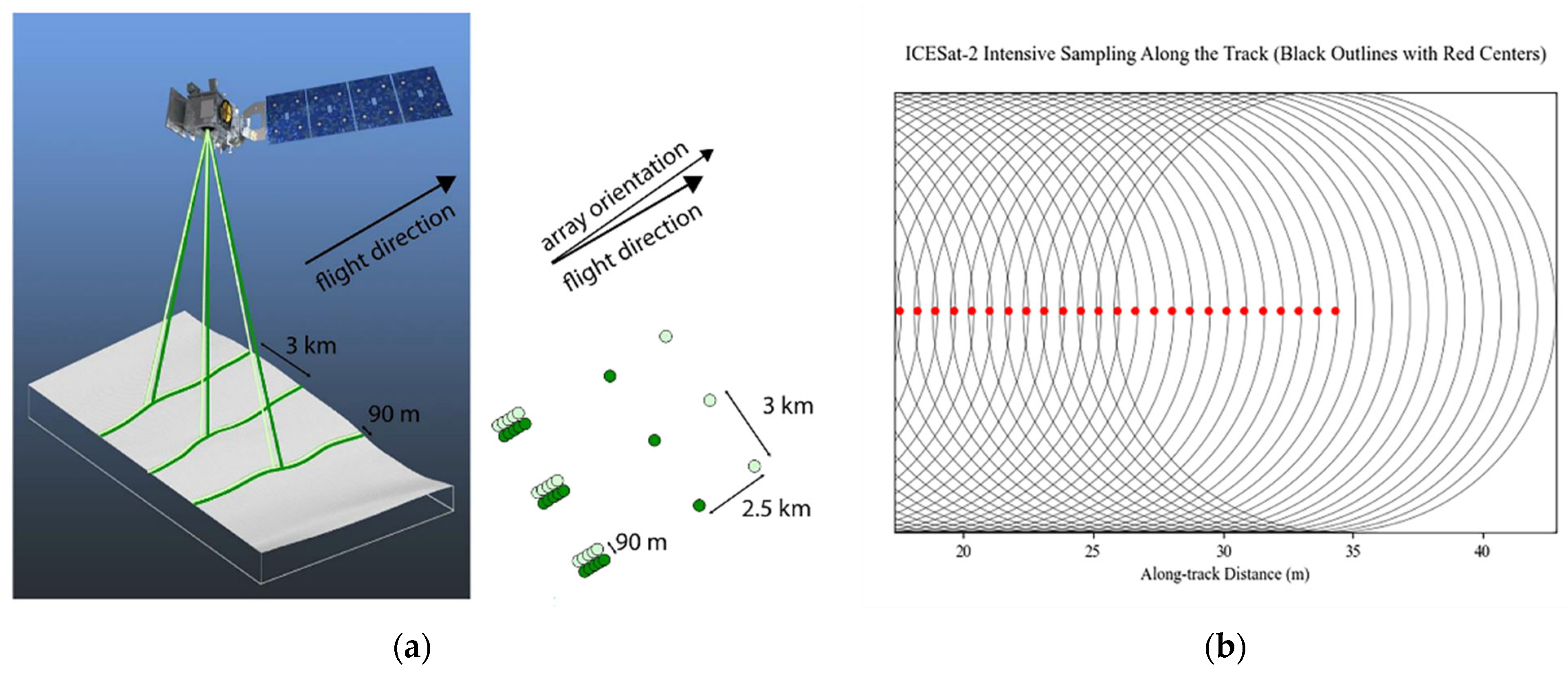
2.2.1. ICESat-2 Data

This study utilized the ATL03 Version 6 dataset, which offers substantial improvements over earlier versions (V3–V5) through enhanced photon classification algorithms and improved geolocation accuracy, achieving a vertical accuracy of ±3.5 cm under clear-sky conditions. To ensure phenological consistency with the LiCHy airborne LiDAR data, ICESat-2 observations collected between April 2021 and December 2023 were extracted. Temporal matching was conducted based on the seasonal acquisition window of the LiCHy data, spanning from spring leaf-out to autumn leaf-fall. It is noteworthy that from April 4 to April 12, 2022, ATLAS ceased data acquisition due to a spacecraft attitude control anomaly that triggered safe mode, as reported in the NASA operational status report (2022–0412). Consequently, ICESat-2 observations are unavailable for this period.

The ground configuration of the ATLAS six-beam system is illustrated in Figure 2a. Each strong–weak beam pair is spaced 2.5 km apart along-track and 3 km apart cross-track, with an individual beam footprint diameter of 17 m (Figure 2b). This configuration enables three-dimensional characterization of complex terrain by combining high-frequency sampling (0.7 m per point) with multi-angle coverage, achieving planar positioning accuracy of <6.5 m [24]. The key system parameters are summarized in

Table 1. ICESat-2 technical parameters overview.

Category	Parameter	Indicator/Value	Remarks
Satellite Basic Information	Launch Date	15 September 2018
	Operating Agency	NASA
	Design Life	3 years	Still operational as of 2024
	Orbit Type	Near-polar sun-synchronous
	Orbit Altitude	~496 km
	Orbit Inclination	92°
	Revisit Period	91 days
Payload (ATLAS)	Laser Wavelength	532 nm (green light)
	Laser Pulse Frequency	10 kHz	10,000 laser pulses per second
	Number of Beams	6 beams	3 beam pairs, each with a strong and weak beam
	Beam Pair Spacing (Across-track)	~3.3 km
	Beam Spacing Within Pair	~90 m
	Vertical Accuracy	<10 cm	Depends on terrain and system calibration
	Footprint Size (Ground)	~17 m	Diameter of each laser spot
Data Product Parameters	Along-track Resolution	~0.7 m	At single photon level
	Vertical Resolution	Sub-meter (<1 m)
	Data Coverage	Global	Emphasis on polar regions, oceans, and land
	Data Update Frequency	Every 3 months	Updated global coverage of major areas
Key Performance Indicators	Terrain Elevation Measurement Accuracy	Ice Surface: <4 cm; Land Surface: <5 cm; Sea Surface: <2 cm	Depends on surface type and atmospheric conditions
	Vegetation Canopy Penetration	Yes
	Data Product Format	HDF5	Includes latitude, longitude, elevation, timestamp, etc.

, including laser energy, pulse repetition frequency, and related specifications. Notably, the strong-to-weak beam energy ratio of 4:1 provides the physical foundation for discriminating vegetation signals (to which the weak beams are more sensitive) from ground signals (better captured by the strong beams) [25].

2.2.2. LiCHy Airborne LiDAR Data

High-precision airborne Light Detection and Ranging (LiDAR) data, acquired by the LiCHy (LiDAR-CCD-Hyperspectral) integrated airborne remote sensing observation system of the Chinese Academy of Forestry between December 2022 and January 2023, served as the benchmark dataset for this study. These data provided a reliable reference for validating the spaceborne LiDAR-derived Digital Elevation Model (DEM) and Canopy Height Model (CHM). The LiCHy system was equipped with a RIEGL LMS-Q680i LiDAR sensor, operating at a 1550 nm (near-infrared) wavelength. Data were efficiently collected from a flight altitude of 851 m, utilizing a ±30° field-of-view scanning mechanism and a 200 kHz pulse repetition frequency. This configuration yielded a point cloud density of 2 points/m² per single flight strip, which increased to an average of 5 points/m² following multi-strip mosaicking; maximum local densities exceeded 10 points/m², thus meeting the criteria for sub-meter terrain modeling.

Comprehensive data processing was performed using the LiDAR360 software (version 8.0.0.1) platform, incorporating rigorous quality control steps such as point cloud registration and noise removal. Terrain extraction was accomplished using the Iterative Progressive TIN Densification (IPTD) algorithm, chosen for its efficacy in accurately delineating terrain features from discrete return data (LAS 1.2 format). The IPTD algorithm constructs a DEM by iteratively densifying a Triangulated Irregular Network (TIN) seeded with the lowest elevation points, complemented by a highest-point grid interpolation method for surface generation. The resultant 1 m resolution DEM, CHM, and Digital Surface Model (DSM) products were georeferenced to the Universal Transverse Mercator (UTM) coordinate system, with elevations referenced to the World Geodetic System 1984 (WGS84) ellipsoid. Cross-validation against ground control points confirmed the high quality of these airborne LiDAR products, with a planar positioning root mean square error (RMSE) of <0.15 m and an elevation accuracy better than 0.1 m, thereby satisfying the requirements for high-precision reference data.

2.2.3. Auxiliary Data

To quantitatively evaluate the influence of key environmental factors—namely slope, canopy cover, and land cover type—on the accuracy of ICESat-2-derived surface terrain and canopy height estimates, this study integrated several auxiliary datasets. Slope and canopy cover metrics were directly derived from the high-resolution DEM and CHM products generated from the LiCHy airborne LiDAR data. Information pertaining to land cover type and Leaf Area Index (LAI) was extracted from Sentinel-2 multispectral imagery. These images, characterized by a 10 m spatial resolution, were radiometrically calibrated and atmospherically corrected prior to analysis. From the Sentinel-2 data, the Normalized Difference Vegetation Index (NDVI) was calculated, and LAI was subsequently estimated using a pixel dichotomy model. Following this, a knowledge-based classification approach was employed to delineate detailed vegetation cover types within the study area, which included forests (further categorized into coniferous, broad-leaved, and mixed sub-types), shrublands, and grasslands. Characteristically, the study area is dominated by coniferous and broad-leaved forests, exhibiting an average tree height of 18.01 m, a mean terrain slope of 28.99°, an average vegetation coverage of 68.74%, and a mean LAI of 3.73.

2.3. ATL03 Data Processing

The processing of ICESat-2 ATL03 data commenced with a critical point cloud denoising step, wherein photon-level classification was performed to differentiate between signal and noise photons. Generally, point cloud classification methodologies can be categorized as either supervised or unsupervised [26]. Supervised techniques, such as Support Vector Machines (SVM), Random Forests, and deep learning models, necessitate extensive labeled training datasets. However, the complex and often unpredictable noise distribution inherent in ICESat-2 data, coupled with the scarcity of readily available labeled data for such applications, renders unsupervised classification methods more practical and commonly adopted.

Density-Based Spatial Clustering of Applications with Noise (DBSCAN) is a widely used unsupervised clustering algorithm. In this study, considering the distinct spatial distribution of signal and noise photons and the non-uniform noise patterns present in ICESat-2 data over complex terrain, an adaptive DBSCAN algorithm enhanced by extended Bayesian decision theory (BDT-ADBSCAN), as proposed by Mei et al. [27], was applied. This algorithm was selected for its demonstrated ability to address heterogeneous noise characteristics and varying photon densities, particularly in complex environments, without requiring extensive manual parameter tuning as in standard DBSCAN. A major advantage of BDT-ADBSCAN lies in its capacity to dynamically adjust the critical parameters—ε (epsilon, search radius) and MinPts (minimum number of points)—based on local data density. These adjustments are guided by Bayesian decision theory, which estimates the posterior probabilities of photons belonging to signal or noise clusters. This approach enables the algorithm to determine optimal ε and MinPts values adaptively for each region, thereby eliminating the need for global threshold settings and enhancing adaptability to variable photon distributions.

This level of adaptability is essential for robust separation of signal from complex and non-uniform noise in ICESat-2 data, particularly in areas characterized by steep topographic gradients and diverse vegetation structures. The implementation followed the methodology described by Mei et al. [27]. Within the three LiCHy airborne LiDAR validation areas, covering a total of 17.41 km², the initial average density of ICESat-2 ATL03 photons was approximately 18,924 points/km². After the application of the BDT-ADBSCAN classification algorithm to distinguish signal photons from noise, the average density of retained signal photons for subsequent analysis was approximately 1907 points/km².

From the classified signal photons, Relative Height (RH) metrics, representing height percentiles of LiDAR energy return above the estimated ground (e.g., RH90, RH100), were derived to characterize canopy vertical structure and aid in canopy height estimation.

Subsequent to photon classification, identified signal photons were utilized for the derivation of canopy height. The accurate determination of canopy height is contingent upon the effective alignment of sampling window dimensions with the local canopy scale [28,29]. To overcome the limitations associated with conventional fixed-window approaches, this study implemented an adaptive search strategy for the optimal selection of terrain reference points. This strategy dynamically optimizes the search for ground returns corresponding to each canopy photon, rather than relying on fixed-length segmentation. Specifically, for each potential canopy photon, the algorithm initiated a search for terrain reference points within an initial radius of 50 m, progressively expanding this radius up to a maximum of 200 m, until a minimum of three suitable terrain points (nearby_ground ≥ 3) were identified. To refine the accuracy of the local terrain elevation estimate, a distance-weighting scheme was applied to these identified terrain reference points, assigning greater influence to closer points. Further quality control measures were instituted: (i) a minimum of three valid terrain reference points were required for the estimation of terrain elevation beneath each canopy photon; (ii) a standard DBSCAN algorithm (ε = 5 m, MinPts = 2) was subsequently used to filter out anomalous terrain points from the selected local set; and (iii) the interquartile range (IQR) method (1.5 × IQR criterion) was applied to detect and remove outlier canopy height values. For computational efficiency, the final terrain elevation at each point was calculated using a distance-weighted averaging approach within an enlarged smoothing window to mitigate residual noise effects. A detailed flowchart illustrating the complete ATL03 data processing workflow is presented in Figure 3.

2.4. Accuracy Assessment

To assess the accuracy of ICESat-2 terrain and canopy height measurements, this study employed statistical metrics calculated using reference values derived from LiCHy DEM and CHM products. The metrics utilized include (1) bias, (2) mean absolute error (MAE), (3) coefficient of determination (R²), (4) root mean square error (RMSE), and (5) percentage root mean square error (%RMSE).

$$Bias={\displaystyle \frac{1}{n}}\sum _{i=1}^n\left(x_i-y_i\right)$$

(1)

$$MAE={\displaystyle \frac{1}{n}}\sum _{i=1}^n\left|x_i-y_i\right|$$

(2)

$$R^2=1-{\displaystyle \frac{\sum _{i=1}^n{\left(x_i-y_i\right)}^2}{\sum _{i=1}^n{\left(x_i-\overline{y}\right)}^2}}$$

(3)

$$RMSE=\sqrt{{\displaystyle \frac{1}{n}}\sum _{i=1}^n{\left(x_i-y_i\right)}^2}$$

(4)

$$\mathrm{\%}\mathrm{R}\mathrm{M}\mathrm{S}\mathrm{E}={\displaystyle \frac{RMSE}{\overline{y}}}\times 100\%$$

(5)

In the equation, $x_i$ represents the terrain or canopy height observations obtained by ICESat-2, $y_i$ represents the reference elevation or canopy height data generated by the LiCHy airborne LiDAR system, $n$ represents the total number of samples, and $\overline{y}$ represents the average value of the reference elevation or canopy height.

3. Results

3.1. Assessment of Photon Classification Performance

The precise classification of photon data is a fundamental prerequisite for the accurate derivation of understory terrain and canopy height metrics from ICESat-2/ATLAS data, as it directly influences the fidelity of subsequent retrievals. In complex forested terrains, both photon penetration through the canopy and the subsequent classification of returns present considerable challenges. As illustrated in Figure 4a, a significant portion of emitted photons are scattered at the canopy top or within the canopy volume. This scattering results in a sparser distribution of photons reaching the ground, which complicates understory terrain measurement [30] and reflects the substantial interference imposed by complex forest structures on laser photon penetration. Notwithstanding these difficulties, the employed BDT-ADBSCAN algorithm demonstrated effective identification of ground photons, yielding a terrain profile generally consistent with that derived from the LiCHy DEM. This consistency substantiates the potential of ICESat-2 for ground detection even under such challenging terrain conditions.

A comparative analysis of the photon distributions shown in Figure 4b (strong beam) and Figure 4c (weak beam) clearly highlights the modulating effect of beam energy on penetration capability. The strong beam, characterized by a transmit energy approximately four times greater than that of the weak beam (details in Table 1), exhibited markedly enhanced ground detection performance. For instance, in a cliff area with a 42° slope (depicted in Figure 4a), ground photons acquired by the strong beam demonstrated a tendency to cluster along the slope-normal direction, indicative of improved signal stability and penetration depth. Furthermore, the higher photon flux associated with the strong beam facilitated deeper penetration through multiple canopy layers, a phenomenon evidenced by the vertically extended distribution of photon returns in Figure 4b. Conversely, photons from the weak beam were predominantly intercepted by the upper canopy strata, with most signal returns concentrated 2–4 m below the canopy top (Figure 4c). This resulted in a higher omission rate for ground photons and, consequently, a reduction in the completeness of the retrieved terrain surface.

Further examination of Figure 4c reveals instances where multiple classified photon types (including those identified as ground photons (red dots) and vegetation photons (green dots)) are located significantly below the reference DTM profile. Such occurrences lead to substantial underestimation of both terrain elevation and, consequently, canopy height. This observation points to considerable classification uncertainty and a degradation in accuracy when processing weak-beam data, particularly under steep terrain conditions. In environments characterized by complex forest architecture and high canopy density, strong-beam data consistently provided a more comprehensive characterization of both forest and underlying terrain structures. Specifically, in regions with tall canopies, strong beams were able to penetrate multiple canopy layers more effectively, thereby acquiring a greater number of ground photons and enhancing the capability for precise retrieval of both forest structural attributes and terrain elevation.

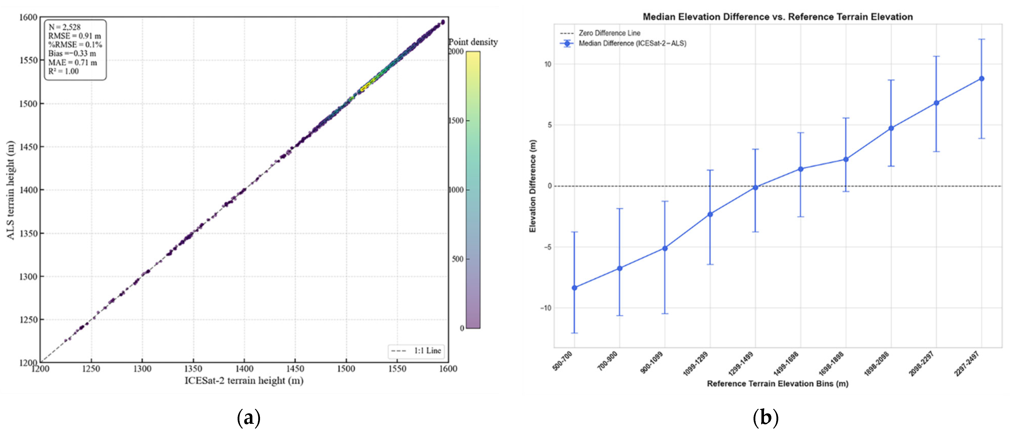
3.2. Terrain Height Validation

The performance of ICESat-2 in retrieving terrain height under complex terrain and diverse vegetation conditions was rigorously validated using high-precision reference elevation data derived from the LiCHy airborne LiDAR system. Within the study area (Figure 1), terrain heights were extracted from the ICESat-2/ATL03 product. These estimates were then compared against the reference terrain data derived from the LiCHy system. A total of 2528 ATL03 terrain height samples were selected for this validation, and standard statistical metrics were computed to quantify performance (Figure 5).

The validation results revealed a high degree of consistency between ICESat-2-derived terrain heights and the LiCHy DEM. The scatter plot (Figure 5a) depicted a strong linear relationship, closely aligning with the 1:1 line, with data points evenly distributed along this diagonal. An exceptionally high coefficient of determination (R²) of 1.00 was achieved, underscoring the excellent capability of ICESat-2 for terrain measurement in this study area. Specifically, the comparison yielded a mean absolute error (MAE) of 0.71 m and a root mean square error (RMSE) of 0.91 m. Figure 5b shows that ICESat-2 tends to underestimate terrain elevation in lower elevation regions (below 1400 m), with a median difference reaching nearly −10 m. In contrast, at higher elevations (above 1800 m), ICESat-2 slightly overestimates elevation. Overall, the estimates exhibit a systematic elevation-dependent bias but maintain a consistent agreement with the reference ALS data.

It is important to note that the overall RMSE of 0.91 m (Figure 5a) represents the performance of the aggregated dataset following the complete processing workflow. In contrast,

Table 2. Terrain height accuracy across ICESat-2 data types.

Scenario	Bias/m	MAE/m	RMSE/m
Strong	−0.53	2.03	3.34
Weak	0.19	4.54	7.20
Day	−0.12	2.40	4.03
Night	−0.82	2.07	3.39
Strong and day	0.03	2.65	4.92
Weak and night	−1.97	3.93	7.34
Weak and day	5.29	8.04	10.54
Strong and night	−0.74	2.33	4.18

presents a detailed breakdown of accuracy metrics for specific subsets based on original beam strength and acquisition time.

The effects of beam strength (strong vs. weak) and data acquisition time (day vs. night) on terrain height accuracy were examined under eight distinct scenarios, with detailed metrics summarized in Table 2. Beam strength was identified as the primary factor affecting accuracy. As shown in Table 2, strong beams yielded significantly higher accuracy than weak beams, with RMSE and MAE reduced by 53.6% and 55.3%, respectively. This substantial improvement is mainly attributed to the higher photon flux of strong beams, which enhances their ability to penetrate vegetation and detect ground returns.

The effect of observation time (day vs. night) on accuracy was found to be beam-strength dependent (Table 2). Strong beams exhibited relatively stable performance across both day and night conditions, with nighttime acquisitions improving RMSE by 15.0% compared to daytime. In contrast, weak beams were more sensitive to observation time, showing a 30.4% reduction in RMSE at night. These findings suggest that weak beams are more susceptible to solar background noise during daytime acquisitions.

Further investigation into systematic biases revealed distinct differences across the data acquisition scenarios (Table 2). While strong beams generally showed a slight underestimation (Bias = −0.53 m) and weak beams a slight overestimation (Bias = 0.19 m), the “Weak and day” scenario exhibited the most pronounced positive bias (+5.29 m) and the highest RMSE (10.54 m). This notably poorer performance is attributed to the compounded effect of low signal energy from weak beams and high solar background noise during daytime, which severely degrades the Signal-to-Noise Ratio (SNR). Such conditions significantly increase the difficulty of accurately classifying ground photons, often leading to the misidentification of low canopy returns as terrain. In contrast, nighttime strong-beam (MAE = 2.33 m) and daytime strong-beam (MAE = 2.65 m) scenarios yielded the highest accuracy, underscoring the robustness of strong beams. The stark difference in performance, with the “Weak and day” MAE (8.04 m) being approximately 3.5 times higher than the best-performing scenario, highlights the critical impact of observation conditions on ICESat-2 terrain height accuracy.

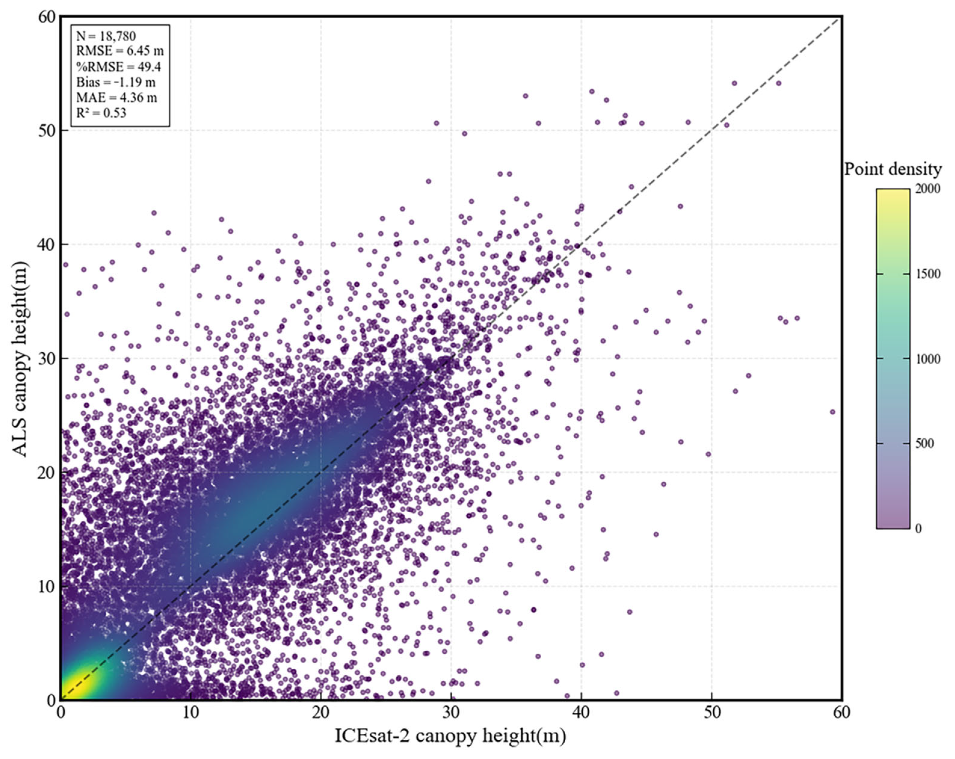
3.3. Canopy Height Validation

Comparative analysis of ICESat-2 canopy height with airborne laser scanning (ALS) reference data (Figure 6) indicates a moderate correlation between the two (R² = 0.53). The scatter distribution shows a significant systematic bias, with ICESat-2 measurements generally lower than the reference line, with an overall bias of −1.19 m. Statistical indicators show that this dataset (N = 18,780) has an RMSE of 6.45 m, a relative error of 49.4%, and an MAE of 4.36 m, indicating substantial uncertainty in ICESat-2 canopy height estimation. Particularly in high canopy regions (>30 m), data points exhibit increased dispersion, suggesting that measurement accuracy decreases as canopy height increases.

Accuracy analysis across different data types, with detailed metrics presented in

Table 3. Accuracy of ICESat-2-derived maximum canopy height across different data types.

Scenario	Bias/m	MAE/m	R2	RMSE/m	%RMSE
Strong	−1.22	4.19	0.57	6.2	47.7%
Weak	−1.02	5.27	0.33	7.70	58.5%
Day	−1.72	4.84	0.40	6.98	54.9%
Night	−0.66	3.84	0.53	5.82	44.0%
Strong and day	−1.62	4.81	0.42	6.95	53.5%
Weak and night	−0.23	5.31	0.30	7.85	56.5%
Weak and day	−2.23	5.20	0.29	8.37	63.0%
Strong and night	−0.62	3.59	0.56	5.41	41.7%

, revealed significant effects of beam strength and observation time on canopy height estimation. Specifically, strong-beam data (RMSE = 6.20 m) exhibited higher accuracy than weak-beam data (RMSE = 7.70 m), while nighttime acquisitions (RMSE = 5.82 m) outperformed those collected during the day (RMSE = 6.98 m), with a lower overall bias (Table 3). The highest accuracy was achieved under nighttime strong-beam conditions (RMSE = 5.41 m, MAE = 3.59 m), whereas the poorest performance occurred with daytime weak-beam data (RMSE = 8.37 m). These findings highlight the pivotal roles of beam energy and background noise in influencing the accuracy of ICESat-2 canopy height retrievals. Strong beams, with higher photon flux, enhance the detection of forest vertical structure, while nighttime conditions reduce solar background interference, thereby improving signal quality. The consistent underestimation observed across all scenarios (Table 3) likely reflects the intrinsic limitations of ICESat-2 in penetrating dense forest canopies, especially in structurally complex, tall-vegetation regions.

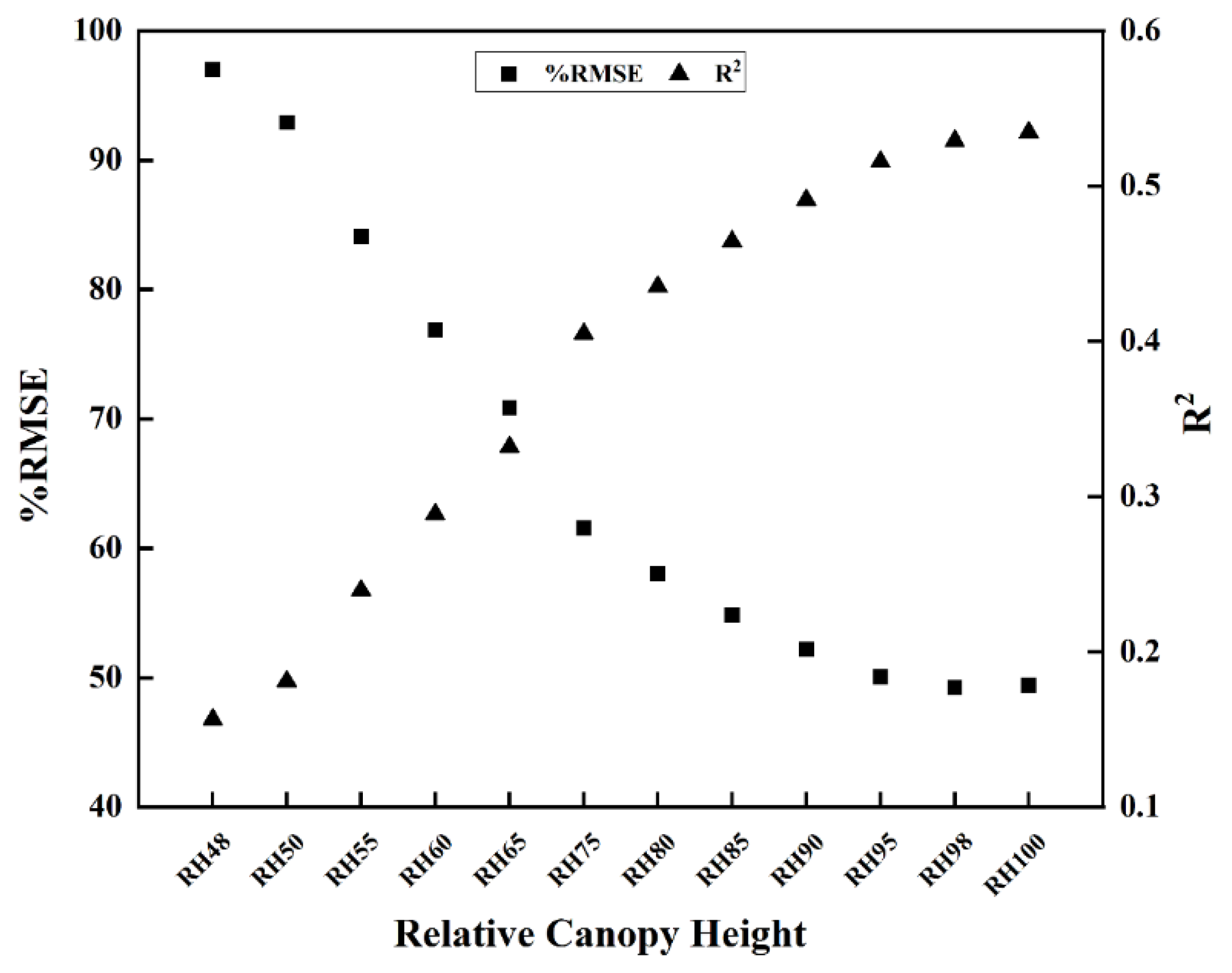
3.4. Influence of Relative Height Metrics on Canopy Height Accuracy

Figure 7 presents the influence of RH on forest canopy height estimation accuracy. Results indicate that %RMSE and R² exhibit opposite trends with changes in RH values. The %RMSE shows a significant decreasing trend as RH values increase, dropping from 97% at RH48 to 49% at RH100. This decreasing trend is particularly pronounced in the RH48-RH75 range and becomes more gradual after RH75, with %RMSE stabilizing at approximately 50% in the RH90–RH100 range. Conversely, R² steadily increases with rising RH values, from 0.15 at RH48 to 0.53 at RH100, with an accelerated growth rate particularly in the RH75–RH90 range, after which it plateaus. At RH90, as %RMSE decreases to approximately 50%, R² reaches 0.51, indicating that this percentile likely represents a critical characteristic of forest canopy structure in the study area. Based on these findings, selecting high-percentile metrics within the RH90–RH100 range has significant implications for improving forest canopy height estimation accuracy.

4. Discussion

4.1. Uncertainty Analysis of Terrain and Canopy Height Estimations

This study investigates key factors influencing the accuracy of ICESat-2 terrain and canopy height retrievals using data from Figure 5 and Figure 6. The analysis employed the Huber loss function [31,32], a robust metric that integrates characteristics of both mean square error (MSE) and mean absolute error (MAE). This function mitigates the impact of extreme outliers prevalent in complex forest canopies while retaining sensitivity to systematic estimation biases. As a normalized metric independent of sample size, the Huber loss value facilitates direct comparisons of accuracy across diverse datasets. The investigated factors include slope, vegetation cover type (e.g., deciduous vs. coniferous), topographic complexity, environmental characteristics, and ICESat-2 laser measurement beam types (e.g., strong vs. weak). Results demonstrate that uncertainties in terrain and canopy height retrievals exhibit distinct patterns.

For terrain height retrieval (Figure 8a), among terrain and environmental characteristic variables (Class I) in the study area, slope exhibited the highest Huber loss value (approximately 0.6 m), indicating that slope is the main factor affecting accuracy in terrain height retrieval. This finding aligns with Tang et al. [33] and He et al. [34], who also identified slope as a key terrain parameter constraining terrain height measurement accuracy. In comparison, the impacts of vegetation coverage and terrain ruggedness were relatively minor, with Huber loss values below 0.4 m. Among ICESat-2 laser measurement beam types (Class II), weak beams showed significantly higher uncertainty than other beam types, with loss values reaching 1.6 m, which may be attributed to signal scattering characteristics of weak beams under complex terrain conditions [17].

For canopy height retrieval (Figure 8b), overall Huber loss values were significantly higher than those for terrain height retrieval. Among Class I factors, canopy height showed the most significant impact, with a Huber loss value reaching 4.2 m, reflecting that the structural complexity of tall vegetation itself is the main source of measurement uncertainty. The impact of other terrain and environmental characteristic factors was relatively small, with Huber loss values generally fluctuating between 3–4 m. Among Class II factors, weak beams similarly exhibited the highest uncertainty (4.5 m), consistent with the trend observed in terrain height retrieval results. This result indicates that although laser beam type affects measurement accuracy, the characteristics of the canopy itself (especially canopy height) are the key factors determining estimation accuracy. Li et al. [35] and Liu et al. [18] also emphasized this finding; through analysis of ICESat-2 data across various vegetation types, they discovered a significant positive correlation between canopy height, vertical structural complexity, and estimation errors, indicating that tall, structurally complex canopies intrinsically present fundamental challenges to precise estimation.

4.2. Analysis of Factors Affecting Terrain Elevation Retrieval Accuracy

This study reveals the mechanism of environmental factors influencing LiDAR elevation measurement accuracy through analyzing the distribution characteristics of terrain height residuals (Figure 9) and root mean square errors (Figure 10). Results indicate that terrain relief is the most significant factor affecting elevation measurement accuracy, followed by vegetation structural characteristics. Unlike previous studies [36,37] that adopted slope filtering thresholds (>10°), this study retains full slope data (0–90°). Although this strategy increases the overall RMSE by approximately 18.6%, it effectively avoids the assessment bias caused by terrain filtering in traditional methods, systematically revealing the true performance boundaries of spaceborne photon LiDAR in complex terrain areas and providing key benchmark references for elevation inversion in extreme terrains such as mountains and canyons.

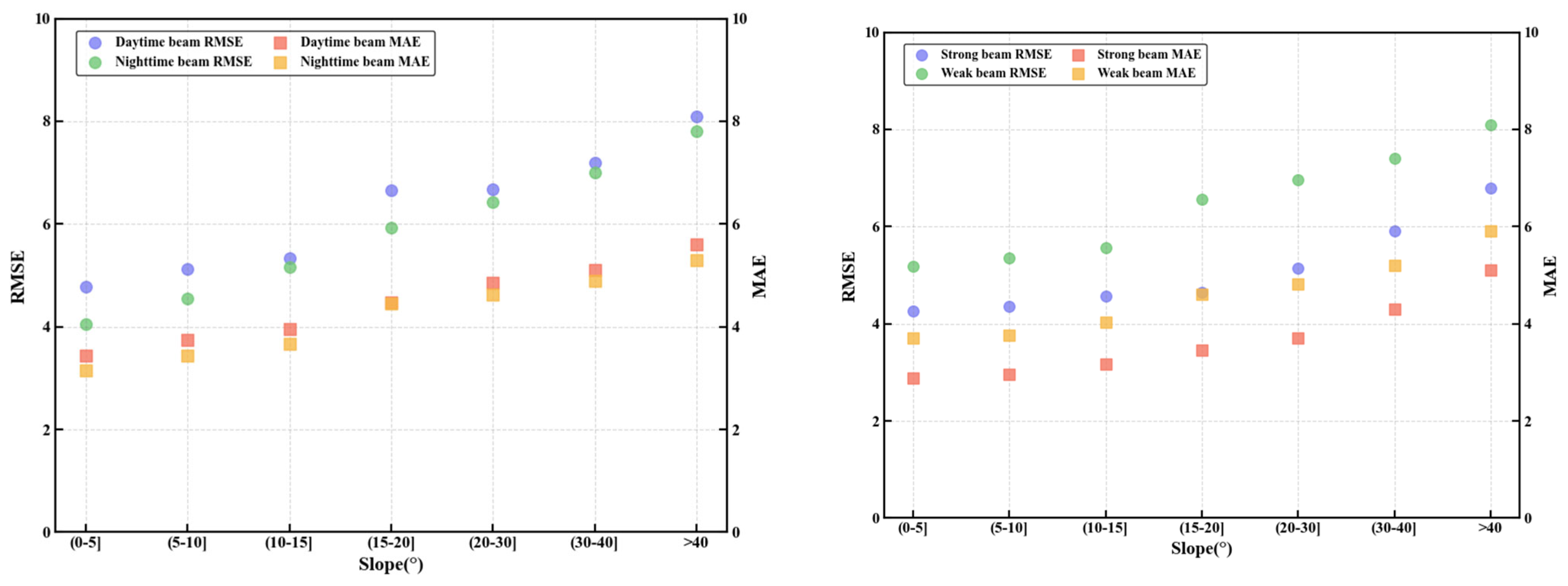
4.2.1. Analysis of Terrain Slope Effects

The distribution of residuals shown in the box plot (Figure 9) demonstrates that in areas with slopes exceeding 20°, the range of residual distribution expands significantly, which is consistent with findings by Liu et al. [18]. This is primarily because steep terrain increases the projected area of laser signals on the ground while simultaneously enhancing multiple scattering effects due to complex topography, both collectively reducing the accuracy of terrain feature extraction. Notably, nighttime observation accuracy in flat areas significantly outperforms daytime measurements, which is related to the interference of solar background radiation on signal-to-noise ratio. Daytime sunlight increases background noise, reducing the capability to detect weak signals, whereas lower background noise at night helps improve the sensitivity of signal detection thresholds [38]. Magruder and Brunt [39] indicate that both point cloud density and accuracy of nighttime observations are superior to daytime observations, especially in flat areas.

4.2.2. Analysis of Canopy Height Effects

Canopy height exhibits a clear threshold effect on ICESat-2 terrain elevation measurement accuracy (third row of Figure 10), with error rates increasing dramatically when canopy heights exceed 20 m. This threshold phenomenon may be related to multiple scattering and energy attenuation of laser signals caused by increased complexity of vegetation vertical structure. Tall forest canopies not only increase the signal transmission path but also increase the probability of laser energy being intercepted by vegetation components, reducing the proportion of effective signals reaching the ground [16,17,40].

The performance difference between ICESat-2’s strong beam (high energy density) and weak beam (low energy density) is significant: the strong beam outperforms the weak beam at various canopy heights due to its higher energy and stronger vegetation penetration capability. This indicates that laser pulse energy is a key factor determining the vegetation penetration capability of signals [41], with higher energy density enabling strong beams to maintain higher ground return signal strength in complex vegetation environments. This conclusion is also verified in the photon classification results of ICESat-2 strong and weak beams in Figure 4, where strong beams maintain a higher proportion of ground return signals after penetrating vegetation.

4.2.3. Analysis of Vegetation Coverage and Density Effects

Land cover classification and LAI analysis further confirm the relationship between vegetation complexity and measurement errors. In areas with simple vegetation structure (such as grasslands and shrublands), the RMSE values of daytime observations are below 1.5 m, while in complex vegetation areas (such as forests), RMSE values reach 3–4 m. This difference can be attributed to differences in vertical structure and changes in optical properties of different vegetation types, with multi-layered canopy structures of forests increasing the complexity of laser signal scattering paths [42].

Vegetation density and measurement accuracy exhibit a non-linear relationship: daytime and nighttime observation RMSE values in areas without vegetation are 0.8 m and 1.2 m, respectively. Within the vegetation coverage range of 20–80%, both daytime and nighttime observation RMSE are maintained at approximately 2.5 m, indicating that observation time has limited impact on measurement accuracy under moderate vegetation conditions. This non-linear relationship reflects the complex modulation effect of vegetation on laser signals, with low-density vegetation mainly weakening signals through scattering, while high-density vegetation may completely block some signals from reaching the ground. LAI analysis shows that RMSE values increase with increasing LAI, and within the lower LAI range (2–3), this relationship is relatively gradual, indicating that within a certain threshold, laser systems can still effectively compensate for signal attenuation caused by vegetation.

4.2.4. Analysis of Day and Night Observation Differences

The accuracy advantage of ICESat-2 nighttime observations mainly stems from reduced solar background radiation and decreased atmospheric turbulence; this advantage is particularly significant in flat terrain and low vegetation areas. In flat terrain, due to simple topography, laser signals experience less interference, and measurement accuracy is further optimized under nighttime conditions. In low vegetation areas, since there is less obstruction of signals by vegetation, the signal-to-noise ratio improves at night, further reducing errors.

Regarding solar background radiation, daytime sunlight increases background noise, reduces signal-to-noise ratio, and impairs weak signal detection capability; at night, background noise is significantly lower, facilitating improved detection of weak signals. Atmospheric scattering and solar radiation have been confirmed as the main sources of background noise in ICESat-2 data; therefore, algorithmic removal of background noise is a key step in data preprocessing [43]. Additionally, the atmosphere is more stable at night with reduced turbulence, which may decrease laser beam scattering and diffusion in the atmosphere, enhancing signal transmission efficiency. As Moudrý et al. [44] pointed out, nighttime atmospheric conditions are more conducive to laser signal transmission. Although changes in vegetation physiological activity may have a slight impact, considering that ICESat-2 uses green light (532 nm), its effect may be limited.

4.3. Analysis of Factors Affecting Canopy Height Retrieval Accuracy

4.3.1. Analysis of Terrain Slope Effects

This study systematically reveals the influence of terrain and vegetation parameters on ICESat-2 canopy height inversion errors through box plots in Figure 11 and scatter distributions in Figure 12. As slope increases, the dispersion degree of error distribution significantly increases, with the median showing an upward trend, particularly when the slope exceeds 30°, where the error dispersion becomes more pronounced (Figure 11a). Scatter plot analysis confirms this trend and reveals that the error growth rate and data dispersion of weak beams are both higher than those of strong beams (first row of Figure 12).

This phenomenon stems from the synergistic effects of geometric distortion and signal attenuation on inversion errors due to terrain slope. When slopes exceed the critical threshold of 30°, the geometric projection area of laser footprints expands, resulting in decreased surface energy density according to the Lambertian scattering model [45]. Simultaneously, micro-topographic shadowing effects caused by terrain undulations are significantly intensified. Theoretical models suggest that weak beams, due to their narrow pulse width (1.5 ns), are more sensitive to pulse broadening caused by terrain, with their signal-to-noise ratio decreasing exponentially with increasing slope (SNR ∝ cos²θ), resulting in greater error dispersion increases for weak beams compared to strong beams. This phenomenon aligns closely with the cosine-squared dependence of echo energy on incidence angle θ in the LiDAR equation [46], revealing the fundamental physical need to consider beam property differences during terrain correction processes.

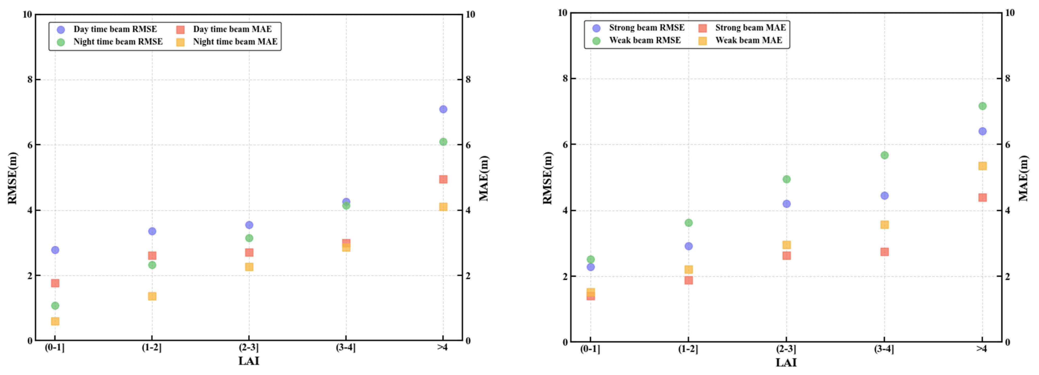
4.3.2. Analysis of Vegetation Coverage and Leaf Area Index Effects

Vegetation coverage and LAI demonstrate common non-linear effects on ICESat-2 measurement performance (Figure 11b,e), reflecting the impact of vegetation structural complexity on laser signal propagation. This influence exhibits distinct bistable characteristics. In moderate vegetation density ranges (coverage 20–60%, LAI 2–3), photon penetration probability and canopy stratification structure achieve dynamic equilibrium, with system errors converging to a theoretical optimal range of ±1.5 m (consistent with the Poisson penetration model [47]).

However, under extreme conditions of low coverage (0–20%) and low LAI (0–1) or high coverage (80–100%) and high LAI (greater than 4), residual fluctuations increase significantly. Photon transport mechanisms undergo phase transitions under low/high-density extreme conditions: low-density areas experience waveform mixing due to multiple surface reflections; high-density areas suffer ground signal loss due to photon attenuation effects according to the Beer–Lambert law [48,49]. Scatter analysis further reveals significant differences in this non-linear effect between strong and weak beams, with weak beams exhibiting significantly increased error variability in areas of high vegetation coverage and high LAI. This is likely because high-density vegetation increases laser signal scattering and absorption, creating complex echo patterns that increase the difficulty of distinguishing between ground and canopy top returns.

4.3.3. Analysis of Canopy Height Effects

The effect of canopy height on retrieval accuracy is particularly pronounced. The box plot in Figure 11c indicates that as canopy height increases, residuals not only show an overall upward trend but are also accompanied by significant positive bias; specifically, when canopy height increases from 0–5 m to >30 m, the average positive bias increases from 2.1 m to 7.8 m, while the maximum residual value rises from 5.4 m to 30.5 m. The scatter plot in Figure 12 further quantitatively confirms this trend, showing that RMSE reaches 8.6 m under high canopy (>30 m) conditions, while it is only 4.8 m under low canopy (0–5 m) conditions.

This height-dependent bias is consistent with findings from Pang et al. [50] and Liu et al. [18]; however, the bias observed in this study for high canopies (>30 m) is more pronounced, possibly due to higher vertical structural complexity within the study area. When canopy height exceeds 30 m, the probability of multiple scattering and delayed return of laser photons within the vegetation layer increases significantly, causing delayed arrival times for some ground photons, resulting in positive bias in height measurements. This phenomenon differs from the ‘backward shift’ in waveform LiDAR, but manifests as a trailing effect in the spatial distribution of photons, thereby producing systematic height overestimation.

Comparisons under day/night and strong/weak-beam conditions (Figure 12) show significant differences: the RMSE of nighttime measurements is on average 0.6 m lower than daytime measurements, which may be attributed to more stable atmospheric conditions at night and reduced background noise. Strong beams show lower MAE than weak beams across all height categories (average reduction of 18.3%); however, in high canopies (>30 m), this advantage diminishes to only 9.7%, indicating the dominant effect of laser energy attenuation under high canopies.

4.3.4. Analysis of Vegetation Type Effects

Different vegetation types exhibit significant and systematic differences in ICESat-2 canopy height retrieval accuracy. The box plot in Figure 11d clearly illustrates the trend in residual distribution from low vegetation (shrubs, grasslands) to complex forest structures (mixed forests, coniferous forests, broadleaf forests, and tropical rainforests). Quantitative analysis indicates that the standard deviations of residuals for grassland and shrub areas are 1.8 m and 2.2 m, respectively, while those for mixed forests, coniferous forests, broadleaf forests, and tropical rainforests reach 5.1 m, 5.3 m, 5.4 m, and 6.7 m, respectively, demonstrating a positive correlation between structural complexity and measurement uncertainty.

The scatter plot in Figure 12 further reveals the differential effects of vegetation types under various observational conditions. Tropical rainforest areas exhibit the highest RMSE values (reaching 9.7 m under weak-beam conditions), while grassland areas show the lowest RMSE (only 2.3 m for nighttime measurements). Notably, although coniferous and broadleaf forests in the study area have similar average heights (23.7 m and 24.2 m, respectively), the MAE value for coniferous forests (4.0 m) is significantly lower than for broadleaf forests. This difference is attributed to the conical structure of coniferous forests forming relatively regular “collimated transmission channels”, enabling more photons to directly reach the ground and return. In contrast, the irregular leaf arrangement in broadleaf forests leads to enhanced isotropic scattering, reducing the detection probability of ground photons [51,52], particularly under weak-beam conditions. The impact of these structural differences on photon transport has been predicted in theoretical models [53], and this study provides empirical support based on field-measured data.

4.4. Multi-Scale Collaborative Optimization Framework

For interactions between terrain slope and canopy vertical structure, constructing a terrain–vegetation joint correction model is recommended in areas with slopes exceeding 25°, integrating Lambertian scattering energy compensation and three-dimensional photon transport simulation. Specifically, by dynamically adjusting the energy weight of weak beams based on the cosine square of the incidence angle (cos²θ), Sentinel-1 DEM data can be introduced to interpret micro-terrain occlusion features, combined with Monte Carlo methods to quantify photon delay distribution caused by multiple scattering.

In high canopy (>30 m) regions, nighttime strong-beam data should serve as the benchmark dataset, supplemented by GEDI waveform features (e.g., RH98) to constrain photon classification thresholds, thereby reducing systematic overestimation errors in canopy height inversion. Vegetation-specific processing requires establishing correspondence between structural complexity and beam parameters. For coniferous forests, standardized photon penetration channel models can be developed based on their collimated transmission characteristics, while broadleaf forests require canopy top echo correction modules utilizing the Anisotropic Scattering Index (ASI).

For structurally complex vegetation such as tropical rainforests, integrating Sentinel-2 red-edge bands with LAI time-series data is recommended to dynamically correct Beer–Lambert attenuation coefficients through leaf optical property inversion. This approach, coupled with Transformer-based deep learning models, effectively separates mixed echo signals. In high coverage areas (>80%), ground signal loss can be mitigated through joint constraint mechanisms incorporating both photon flight time and spatial distribution parameters.

Observation mode optimization is equally important. For terrain and canopy height inversions, nighttime strong-beam data should be prioritized. In complex areas with slopes exceeding 30° and canopy heights above 30 m, spatiotemporal collaborative observations between ICESat-2 and airborne LiDAR are recommended, using stratified control point registration to suppress systematic errors. Additionally, joint error models incorporating terrain slope and canopy height parameters can quantify error accumulation effects under complex terrain conditions.

5. Conclusions

Based on the latest version of ICESat-2 ATL03 data combined with high-precision LiCHy airborne LiDAR products, this study performed systematic validation and uncertainty analysis of terrain and canopy height retrieval performance under complex terrain and diverse vegetation conditions. The main conclusions are as follows:

(1) ICESat-2 demonstrates excellent terrain elevation retrieval capability under complex terrain conditions (R² = 1.00, RMSE = 0.91 m).

(2) Strong beams maintain higher accuracy and stability across all time periods, while weak beams are significantly affected by solar background noise during daytime observations, resulting in substantially increased errors.

(3) Terrain slope is the primary source of error in terrain height retrieval accuracy, with RMSE exhibiting a linear increasing trend with slope, confirming it as the key topographic parameter constraining measurement accuracy.

(4) For forest canopy height estimation, ICESat-2 demonstrates moderate accuracy (R² = 0.53, RMSE = 6.45 m) with systematic underestimation (mean bias = −1.19 m), with strong beams and nighttime data yielding relatively higher precision.

(5) Higher Relative Height (RH) values effectively enhance the reliability of canopy height estimation, with %RMSE decreasing and R² values increasing with higher RH metrics.

(6) Canopy height itself is the critical factor affecting estimation accuracy (Huber loss value 4.2 m), with measurement errors increasing with canopy height.

(7) Canopy height measurement performance is non-linearly regulated by vegetation coverage and LAI, with optimal performance under moderate vegetation density and significantly increased errors under extreme density conditions.

(8) Vegetation type significantly influences height retrieval accuracy, with stable errors in grassland and shrub areas contrasting with significantly increased variability in forest areas.

(9) Weak beams exhibit particular vulnerability under complex environmental conditions, indicating limited application potential in challenging terrain and vegetation scenarios.

Although this study comprehensively evaluated the performance of ICESat-2 under complex terrain and vegetation conditions, several limitations exist: the validation dataset primarily focuses on the Yunnan mountainous forest area (19.6 km²), and applicability to ecosystems such as tropical rainforests and boreal taiga forests requires further verification; a 1–2 year temporal difference between LiCHy and ICESat-2 data may introduce errors due to phenological changes; and the interference of atmospheric turbulence and cloud scattering on photon positioning has not been quantified.

Given the extended orbital lifetime of the ATLAS system (exceeding design lifetime by 200%), future research recommendations include expanding validation to characteristic regions such as the Qinghai-Tibet Plateau and Amazon Basin; integrating GEDI and Sentinel-1 data to develop multi-scale inversion models; creating deep learning-based canopy-terrain photon separation algorithms to enhance performance in high-density vegetation areas; and establishing an Asian mountainous forest long-term observation network that coordinates satellite-airborne-ground multi-source data, promoting the paradigm shift of LiDAR remote sensing from “static inversion” to “process coupling”, providing technical support for earth system science and carbon neutrality goals.

References

1. Fuller, M.R.; Ganjam, M.; Baker, J.S.; Abt, R.C. Advancing Forest Carbon Projections Requires Improved Convergence between Ecological and Economic Models. Carbon Balance Manag. 2025, 20, 2. [Google Scholar] [CrossRef] [PubMed]
2. Canadell, J.G.; Raupach, M.R. Managing Forests for Climate Change Mitigation. Science 2008, 320, 1456–1457. [Google Scholar] [CrossRef] [PubMed]
3. Xu, W.; Cheng, Y.; Luo, M.; Mai, X.; Wang, W.; Zhang, W.; Wang, Y. Progress and Limitations in Forest Carbon Stock Estimation Using Remote Sensing Technologies: A Comprehensive Review. Forests 2025, 16, 449. [Google Scholar] [CrossRef]
4. Yang, J.; Swenson, N.G. Height and Crown Allometries and Their Relationship with Functional Traits: An Example from a Subtropical Wet Forest. Ecol. Evol. 2023, 13, e9804. [Google Scholar] [CrossRef]
5. Huang, J.; Yu, Y. Understory Terrain Estimation by Synergizing Ice, Cloud, and Land Elevation Satellite-2 and Multi-Source Remote Sensing Data. Remote Sens. 2024, 16, 4770. [Google Scholar] [CrossRef]
6. Hudak, A.T.; Lefsky, M.A.; Cohen, W.B.; Berterretche, M. Integration of Lidar and Landsat ETM+ Data for Estimating and Mapping Forest Canopy Height. Remote Sens. Environ. 2002, 82, 397–416. [Google Scholar] [CrossRef]
7. Gómez, C.; White, J.C.; Wulder, M.A. Optical Remotely Sensed Time Series Data for Land Cover Classification: A Review. ISPRS J. Photogramm. Remote Sens. 2016, 116, 55–72. [Google Scholar] [CrossRef]
8. Ho Tong Minh, D.; Le Toan, T.; Rocca, F.; Tebaldini, S.; Villard, L.; Réjou-Méchain, M.; Phillips, O.L.; Feldpausch, T.R.; Dubois-Fernandez, P.; Scipal, K.; et al. SAR Tomography for the Retrieval of Forest Biomass and Height: Cross-Validation at Two Tropical Forest Sites in French Guiana. Remote Sens. Environ. 2016, 175, 138–147. [Google Scholar] [CrossRef]
9. Becker, A.; Russo, S.; Puliti, S.; Lang, N.; Schindler, K.; Wegner, J.D. Country-Wide Retrieval of Forest Structure from Optical and SAR Satellite Imagery with Deep Ensembles. ISPRS J. Photogramm. Remote Sens. 2023, 195, 269–286. [Google Scholar] [CrossRef]
10. Chen, X.; Sun, Q.; Hu, J. Generation of Complete SAR Geometric Distortion Maps Based on DEM and Neighbor Gradient Algorithm. Appl. Sci. 2018, 8, 2206. [Google Scholar] [CrossRef]
11. Mo, L.; Zohner, C.M.; Reich, P.B.; Liang, J.; De Miguel, S.; Nabuurs, G.-J.; Renner, S.S.; Van Den Hoogen, J.; Araza, A.; Herold, M.; et al. Integrated Global Assessment of the Natural Forest Carbon Potential. Nature 2023, 624, 92–101. [Google Scholar] [CrossRef] [PubMed]
12. Kutchartt, E.; Pedron, M.; Pirotti, F. Assessment of Canopy and Ground Height Accuracy from Gedi Lidar over Steep Mountain Areas. ISPRS Ann. Photogramm. Remote Sens. Spat. Inf. Sci. 2022, V-3–2022, 431–438. [Google Scholar] [CrossRef]
13. Campbell, M.J.; Eastburn, J.F.; Dennison, P.E.; Vogeler, J.C.; Stovall, A.E.L. Evaluating the Performance of Airborne and Spaceborne Lidar for Mapping Biomass in the United States’ Largest Dry Woodland Ecosystem. Remote Sens. Environ. 2024, 308, 114196. [Google Scholar] [CrossRef]
14. Fayad, I.; Baghdadi, N.; Alcarde Alvares, C.; Stape, J.L.; Bailly, J.S.; Scolforo, H.F.; Cegatta, I.R.; Zribi, M.; Le Maire, G. Terrain Slope Effect on Forest Height and Wood Volume Estimation from GEDI Data. Remote Sens. 2021, 13, 2136. [Google Scholar] [CrossRef]
15. Pronk, M.; Eleveld, M.; Ledoux, H. Assessing Vertical Accuracy and Spatial Coverage of ICESat-2 and GEDI Spaceborne Lidar for Creating Global Terrain Models. Remote Sens. 2024, 16, 2259. [Google Scholar] [CrossRef]
16. Neuenschwander, A.L.; Magruder, L.A. Canopy and Terrain Height Retrievals with Icesat-2: A First Look. Remote Sens. 2019, 11, 1721. [Google Scholar] [CrossRef]
17. Neuenschwander, A.; Guenther, E.; White, J.C.; Duncanson, L.; Montesano, P. Validation of ICESat-2 Terrain and Canopy Heights in Boreal Forests. Remote Sens. Environ. 2020, 251, 112110. [Google Scholar] [CrossRef]
18. Liu, A.; Cheng, X.; Chen, Z. Performance Evaluation of GEDI and ICESat-2 Laser Altimeter Data for Terrain and Canopy Height Retrievals. Remote Sens. Environ. 2021, 264, 112571. [Google Scholar] [CrossRef]
19. Malambo, L.; Popescu, S.C. Assessing the Agreement of ICESat-2 Terrain and Canopy Height with Airborne Lidar over US Ecozones. Remote Sens. Environ. 2021, 266, 112711. [Google Scholar] [CrossRef]
20. Wang, C.; Zhu, X.; Nie, S.; Xi, X.; Li, D.; Zheng, W.; Chen, S. Ground Elevation Accuracy Verification of ICESat-2 Data: A Case Study in Alaska, USA. Opt. Express 2019, 27, 38168–38179. [Google Scholar] [CrossRef]
21. Xing, Y.; Huang, J.; Gruen, A.; Qin, L. Assessing the Performance of ICESat-2/ATLAS Multi-Channel Photon Data for Estimating Ground Topography in Forested Terrain. Remote Sens. 2020, 12, 2084. [Google Scholar] [CrossRef]
22. Wang, T.; Xu, W.; Bao, A.; Yuan, Y.; Zheng, G.; Naibi, S.; Huang, X.; Wang, Z.; Zheng, X.; Bao, J.; et al. Mapping of Forest Structural Parameters in Tianshan Mountain Using Bayesian-Random Forest Model, Synthetic Aperture Radar Sentinel-1A, and Sentinel-2 Imagery. Remote Sens. 2024, 16, 1268. [Google Scholar] [CrossRef]
23. Urbazaev, M.; Hess, L.L.; Hancock, S.; Sato, L.Y.; Ometto, J.P.; Thiel, C.; Dubois, C.; Heckel, K.; Urban, M.; Adam, M.; et al. Assessment of Terrain Elevation Estimates from Icesat-2 and Gedi Spaceborne Lidar Missions across Different Land Cover and Forest Types. Sci. Remote Sens. 2022, 6, 100067. [Google Scholar] [CrossRef]
24. Magruder, L.; Brunt, K.; Alonzo, M. Early ICESat-2 on-Orbit Geolocation Validation Using Ground-Based Corner Cube Retro-Reflectors. Remote Sens. 2020, 12, 3653. [Google Scholar] [CrossRef]
25. Zhu, X.; Ren, Z.; Nie, S.; Bao, G.; Ha, G.; Bai, M.; Liang, P. DEM Generation from GF-7 Satellite Stereo Imagery Assisted by Space-Borne LiDAR and Its Application to Active Tectonics. Remote Sens. 2023, 15, 1480. [Google Scholar] [CrossRef]
26. Zhou, L.; Sun, G.; Li, Y.; Li, W.; Su, Z. Point Cloud Denoising Review: From Classical to Deep Learning-Based Approaches. Graph. Models 2022, 121, 101140. [Google Scholar] [CrossRef]
27. Mei, H.; Mao, L.; Zhang, Y.; Chen, M. Bdt-Adbscan: Adaptive Density-Based Spatial Clustering of Applications with Noise Based on Bayesian Decision Theory for Identifying Clusters with Multi-Densities. In Proceedings of the 2022 IEEE 10th Joint International Information Technology and Artificial Intelligence Conference (ITAIC), Chongqing, China, 17–19 June 2022; pp. 1510–1516. [Google Scholar]
28. Huang, X.; Cheng, F.; Wang, J.; Duan, P.; Wang, J. Forest Canopy Height Extraction Method Based on ICESat-2/ATLAS Data. IEEE Trans. Geosci. Remote Sens. 2023, 61, 1–14. [Google Scholar] [CrossRef]
29. Wu, Z.; Shi, F. Mapping Forest Canopy Height at Large Scales Using ICESat-2 and Landsat: An Ecological Zoning Random Forest Approach. IEEE Trans. Geosci. Remote Sens. 2023, 61, 1–16. [Google Scholar] [CrossRef]
30. Bourgine, B.; Baghdadi, N.; Hosford, S.; Daniels, P. Generation of a Ground-Level DEM in a Dense Equatorial Forest Zone by Merging Airborne Laser Data and a Top-of-Canopy DEM. Can. J. Remote Sens. 2004, 30, 913–926. [Google Scholar] [CrossRef]
31. Balasundaram, S.; Prasad, S.C. Robust Twin Support Vector Regression Based on Huber Loss Function. Neural Comput. Appl. 2020, 32, 11285–11309. [Google Scholar] [CrossRef]
32. Gupta, D.; Hazarika, B.B.; Berlin, M. Robust Regularized Extreme Learning Machine with Asymmetric Huber Loss Function. Neural Comput. Appl. 2020, 32, 12971–12998. [Google Scholar] [CrossRef]
33. Tang, J.; Xing, Y.; Wang, J.; Yang, H.; Wang, D.; Li, Y.; Zhang, A. A Multilevel Autoadaptive Denoising Algorithm Based on Forested Terrain Slope for ICESat-2 Photon-Counting Data. IEEE J. Sel. Top. Appl. Earth Obs. Remote Sens. 2024, 17, 16831–16846. [Google Scholar] [CrossRef]
34. He, L.; Pang, Y.; Zhang, Z.; Liang, X.; Chen, B. ICESat-2 Data Classification and Estimation of Terrain Height and Canopy Height. Int. J. Appl. Earth Obs. Geoinf. 2023, 118, 103233. [Google Scholar] [CrossRef]
35. Li, Y.; Gao, S.; Fu, H.; Zhu, J.; Hu, Q.; Zeng, D.; Wei, Y. Error Analysis and Accuracy Improvement in Forest Canopy Height Estimation Based on Gedi L2a Product: A Case Study in the United States. Forests 2024, 15, 1536. [Google Scholar] [CrossRef]
36. Sithole, G.; Vosselman, G. Experimental Comparison of Filter Algorithms for Bare-Earth Extraction from Airborne Laser Scanning Point Clouds. ISPRS J. Photogramm. Remote Sens. 2004, 59, 85–101. [Google Scholar] [CrossRef]
37. Meng, X.; Currit, N.; Zhao, K. Ground Filtering Algorithms for Airborne Lidar Data: A Review of Critical Issues. Remote Sens. 2010, 2, 833–860. [Google Scholar] [CrossRef]
38. Zhu, X.; Nie, S.; Wang, C.; Xi, X. The Performance of Icesat-2′s Strong and Weak Beams in Estimating Ground Elevation and Forest Height. In Proceedings of the IGARSS 2020—2020 IEEE International Geoscience and Remote Sensing Symposium, Waikoloa, HI, USA, 26 September–2 October 2020; pp. 6073–6076. [Google Scholar]
39. Magruder, L.A.; Brunt, K.M. Performance Analysis of Airborne Photon- Counting Lidar Data in Preparation for the Icesat-2 Mission. IEEE Trans. Geosci. Remote Sens. 2018, 56, 2911–2918. [Google Scholar] [CrossRef]
40. Anderson, K.; Hancock, S.; Disney, M.; Gaston, K.J. Is Waveform Worth It? A Comparison of Li DAR Approaches for Vegetation and Landscape Characterization. Remote Sens. Ecol. Conserv. 2016, 2, 5–15. [Google Scholar] [CrossRef]
41. Zhang, Z.; Ding, J.; Zhu, C.; Wang, J.; Ma, G.; Ge, X.; Li, Z.; Han, L. Strategies for the Efficient Estimation of Soil Organic Matter in Salt-Affected Soils through Vis-NIR Spectroscopy: Optimal Band Combination Algorithm and Spectral Degradation. Geoderma 2021, 382, 114729. [Google Scholar] [CrossRef]
42. Neuenschwander, A.; Magruder, L. The Potential Impact of Vertical Sampling Uncertainty on ICESat-2/ATLAS Terrain and Canopy Height Retrievals for Multiple Ecosystems. Remote Sens. 2016, 8, 1039. [Google Scholar] [CrossRef]
43. Liu, J.; Liu, J.; Xie, H.; Ye, D.; Li, P. A Multi-Level Auto-Adaptive Noise-Filtering Algorithm for Land Icesat-2 Photon-Counting Data. Remote Sens. 2023, 15, 5176. [Google Scholar] [CrossRef]
44. Moudrý, V.; Gdulová, K.; Gábor, L.; Šárovcová, E.; Barták, V.; Leroy, F.; Špatenková, O.; Rocchini, D.; Prošek, J. Effects of Environmental Conditions on ICESat-2 Terrain and Canopy Heights Retrievals in Central European Mountains. Remote Sens. Environ. 2022, 279, 113112. [Google Scholar] [CrossRef]
45. Carrea, D.; Abellan, A.; Humair, F.; Matasci, B.; Derron, M.-H.; Jaboyedoff, M. Correction of Terrestrial Lidar Intensity Channel Using Oren–Nayar Reflectance Model: An Application to Lithological Differentiation. ISPRS J. Photogramm. Remote Sens. 2016, 113, 17–29. [Google Scholar] [CrossRef]
46. Habib, A.F.; Kersting, A.P.; Shaker, A.; Yan, W.-Y. Geometric Calibration and Radiometric Correction of Lidar Data and Their Impact on the Quality of Derived Products. Sensors 2011, 11, 9069–9097. [Google Scholar] [CrossRef]
47. Roy, G.; Tremblay, G. Polarimetric Multiple Scattering LiDAR Model Based on Poisson Distribution. Appl. Opt. 2022, 61, 5507. [Google Scholar] [CrossRef]
48. Knapp, N.; Fischer, R.; Huth, A. Linking Lidar and Forest Modeling to Assess Biomass Estimation across Scales and Disturbance States. Remote Sens. Environ. 2018, 205, 199–209. [Google Scholar] [CrossRef]
49. Qu, Y.; Shaker, A.; Korhonen, L.; Silva, C.A.; Jia, K.; Tian, L.; Song, J. Direct Estimation of Forest Leaf Area Index Based on Spectrally Corrected Airborne Lidar Pulse Penetration Ratio. Remote Sens. 2020, 12, 217. [Google Scholar] [CrossRef]
50. Pang, S.; Li, G.; Jiang, X.; Chen, Y.; Lu, Y.; Lu, D. Retrieval of Forest Canopy Height in a Mountainous Region with ICESat-2 ATLAS. For. Ecosyst. 2022, 9, 100046. [Google Scholar] [CrossRef]
51. Zhang, Z.; Cao, L.; She, G. Estimating Forest Structural Parameters Using Canopy Metrics Derived from Airborne Lidar Data in Subtropical Forests. Remote Sens. 2017, 9, 940. [Google Scholar] [CrossRef]
52. Zhong, H.; Zhang, Z.; Liu, H.; Wu, J.; Lin, W. Individual Tree Species Identification for Complex Coniferous and Broad-Leaved Mixed Forests Based on Deep Learning Combined with Uav Lidar Data and Rgb Images. Forests 2024, 15, 293. [Google Scholar] [CrossRef]
53. Swatantran, A.; Tang, H.; Barrett, T.; DeCola, P.; Dubayah, R. Rapid, High-Resolution Forest Structure and Terrain Mapping over Large Areas Using Single Photon Lidar. Sci. Rep. 2016, 6, 28277. [Google Scholar] [CrossRef]
Figure 1. Overview of the study area: (a) location within China, (b) position within Yunnan Province, (c) ICESat-2 laser footprints and airborne LiDAR data coverage in the Pu’er study area. In panel (c), green points represent ICESat-2 laser footprints (signal photons after filtering), red points represent airborne LiDAR sampling point locations, and the grayscale background displays the digital elevation model (DEM) generated from airborne LiDAR data.
Remotesensing 17 01897 g001
Figure 2. Geometric layout of ICESat-2 ATLAS instrument ground footprints and along-track sampling schematic. (a) Schematic diagram of ICESat-2 multi-beam laser altimetry principle (https://nsidc.org/data/ATL03, accessed on 27 January 2025). (b) Schematic of ICESat-2 along-track footprints and center point distribution.
Remotesensing 17 01897 g002
Figure 3. Adaptive canopy height calculation process for ICESat-2/ATL03 data.
Remotesensing 17 01897 g003
Figure 4. Comparison between ICESat-2 photon classification results and LiCHy reference data under complex terrain conditions. (a) Distribution of photons under complex terrain: red dots represent ground photons, green dots represent vegetation photons, blue dots represent canopy top photons, gray lines represent the DSM derived from LiCHy airborne LiDAR data, and black lines represent the DTM derived from LiCHy airborne LiDAR data; (b) classification results of strong-beam photon signals under steep slope terrain; (c) classification results of weak-beam photon signals under steep slope terrain.
Remotesensing 17 01897 g004aRemotesensing 17 01897 g004b
Figure 5. Accuracy assessment of ICESat-2 terrain elevations using airborne LiDAR data: (a) scatterplot of ICESat-2 versus ALS terrain heights, illustrating overall correlation and point density; (b) median elevation differences (ICESat-2—ALS) across ALS terrain elevation bins, with interquartile range (IQR) error bars.
Remotesensing 17 01897 g005
Figure 6. Accuracy assessment of ICESat-2-derived maximum canopy height based on airborne LiDAR data. The ICESat-2 maximum canopy height (x-axis) is defined as the elevation difference between the highest classified signal photon and the locally refined terrain surface.
Remotesensing 17 01897 g006
Figure 7. Influence of relative canopy height variations on canopy height estimation accuracy (%RMSE and R2).
Remotesensing 17 01897 g007
Figure 8. Huber loss-based accuracy assessment of ICESat-2 (a) terrain elevation and (b) canopy height retrievals. Group I includes terrain and environmental variables, with ‘Canopy Height’ derived from the LiCHy CHM. Group II denotes laser beam types.
Remotesensing 17 01897 g008
Figure 9. ICESat-2 terrain elevation residuals (relative to LiCHy LiDAR data) with varying environmental factors: (a) slope, (b) vegetation cover percentage, (c) canopy height, (d) vegetation cover type, and (e) LAI.
Remotesensing 17 01897 g009
Figure 10. Variations in the RMSE of ICESat-2 terrain height inversion under different environmental factors and beam types.
Remotesensing 17 01897 g010
Figure 11. ICESat-2 canopy height residuals (relative to LiCHy LiDAR data) with varying environmental factors: (a) slope, (b) vegetation cover percentage, (c) canopy height, (d) vegetation cover type, and (e) LAI.
Remotesensing 17 01897 g011aRemotesensing 17 01897 g011b
Figure 12. Characteristics of error variations in ICESat-2 beams across different observation periods (daytime/nighttime) and energy levels: analysis based on parameters including terrain slope, vegetation coverage, canopy height, vegetation type, and LAI.
Remotesensing 17 01897 g012aRemotesensing 17 01897 g012bRemotesensing 17 01897 g012c