Cascade Learning Early Classification: A Novel Cascade Learning Classification Framework for Early-Season Crop Classification

Abstract

Accurate early-season crop classification is critical for food security, agricultural applications and policymaking. However, when classification is performed earlier, the available time-series data gradually become scarce. Existing methods mainly focus on enhancing the model’s ability to extract features from limited data to address this challenge, but the extracted critical phenological information remains insufficient. This study proposes a Cascade Learning Early Classification (CLEC) framework, which consists of two components: data preprocessing and a cascade learning model. Data preprocessing generates high-quality time-series data from the optical, radar and thermodynamic data in the early stages of crop growth. The cascade learning model integrates a prediction task and a classification task, which are interconnected through the cascade learning mechanism. First, the prediction task is performed to supplement more time-series data of the growing stage. Then, crop classification is carried out. Meanwhile, the cascade learning mechanism is used to iteratively optimize the prediction and classification results. To validate the effectiveness of CLEC, we conducted early-season classification experiments on soybean, corn and rice in Northeast China. The experimental results show that CLEC significantly improves crop classification accuracy compared to the five state-of-the-art models in the early stages of crop growth. Furthermore, under the premise of obtaining reliable results, CLEC advances the earliest identifiable timing, moving from the flowing to the third true leaf stage for soybean and from the flooding to the sowing stage for rice. Although the earliest identifiable timing for corn remains unchanged, its classification accuracy improved. Overall, CLEC offers new ideas for solving early-season classification challenges.

1. Introduction

Timely crop classification enables accurate assessment of crop distribution and area, which is critical for yield forecasting and food security assessment [1,2]. However, most studies on crop classification rely on full-year time-series data. This post-season classification, rather than early-season classification, has lower timeliness and cannot provide decision makers with timely data support [3]. In contrast, early-season classification refers to crop classification based on the acquisition of time-series data in the early-to-mid stages of crop growth [4]. The early acquisition of crop planting information is of great value for agriculture-related applications and government decision making. It not only provides reliable spatial information for risk management and crop insurance, but also enables precise intervention and effective management during the early stage of crop growth [5,6,7].

Currently, early-season crop classification methods can be divided into two categories: machine-learning-based methods and deep-learning-based methods. Machine-learning-based methods, which operate without human intervention during training, automatically learn the differences exhibited by various crops in time-series data. This enables these methods to uncover underlying patterns in the data, thereby enhancing the accuracy of crop classification [8,9]. Therefore, machine learning clustering algorithms, such as Random Forest (RF) and Support Vector Machine (SVM), have been utilized in early-season crop classification [10,11,12]. RF has been used in several studies, which ultimately deduced the identifiable timing for rice, corn and soybean [13,14]. Some previous studies have used different clustering algorithms, such as gaussian mixture model [15] and multivariate spatiotemporal clustering [16], to extract the feature information from vegetation index curves and aggregate remote sensing spectral data. These machine-learning-based methods achieved satisfactory overall accuracy in the mid-stages of crop growth. However, these machine-learning-based methods struggle to effectively model the complex nonlinear relationships of temporal dependencies [17]. Consequently, this leads to the inability to achieve accurate classification earlier in the season.

Compared to machine-learning-based methods, deep-learning-based methods are more adept at handling time-series data with complex temporal dependencies and nonlinear relationships. This advantage is primarily attributed to their ability to automatically extract complex features and perform multi-layer nonlinear transformations, enabling effective temporal feature extraction [18]. Therefore, some studies have begun adopting Transformer, Convolutional Neural Networks (CNNs) and Recurrent Neural Networks (RNNs) for early-season crop classification [19,20,21]. Specifically, Transformer-based methods use multi-head attention mechanisms and encoder–decoder structures to extract global information from time-series data [22,23]. In contrast to Transformer, Long Short-Term Memory (LSTM) uses gating mechanisms to represent temporal dependencies over different time spans in recursive connections [24]. For instance, Xu et al. [25] proposed an attention-based bidirectional LSTM for the classification of corn and soybean, which enhanced the ability to capture temporal features. Furthermore, ELECT was proposed to balance the classification of earliness and accuracy [26]. Mask-PSTIN was proposed to effectively aggregate time-series data by combining temporal random masking with pixel set spatial information [27]. These two innovative LSTM-based models, ELECT and Mask-PSTIN, offer new perspectives for early-season crop classification. Nevertheless, these methods focus on extracting global features from time-series data while neglecting local features.

Additionally, several studies have leveraged the local receptive fields and multiple convolution kernels of CNNs to extract local features from time-series data [28,29]. Both 1D-CNN [30] and 3D-CNN [31] have been used to extract local features from time-series data, performing classification for cotton and wheat. To integrate the advantages of LSTM and CNN, Yang et al. [32] proposed the EMET framework that combined the Super-Resolution Convolutional Neural Network (SRCNN) and LSTM to jointly extract global and local features from time-series data.

Nowadays, deep-learning-based methods improve feature extraction and fusion ability by using attention mechanisms, gating mechanisms or convolution operations [27,33]. These enhancements enable the extraction of more critical information, leading to better classification results compared to machine-learning-based methods. However, as classification is performed earlier, time-series data gradually become scarce. This limits the extraction of sufficient critical phenological information using these methods, leading to a decline in classification accuracy. When addressing this limitation, most studies focus on further improving the methods’ ability to extract features from the limited data. Nevertheless, the extracted information remains insufficient. To our knowledge, no approach has tackled this limitation from another perspective: completing the data to create a full-year time series before classification by leveraging accurate predictions.

In this study, we propose a novel idea. Specifically, crop classification is decomposed into two tasks: prediction and classification, which are interconnected through the cascade learning mechanism [34]. In the prediction task, early-season data are utilized to predict future data. Then, the predicted and early-season data are concatenated to provide full-year time-series data for classification, thereby enabling the extraction of more critical phenological information. Meanwhile, the classification results are used to reverse-optimize the accuracy of the prediction task through the cascade learning mechanism.

Based on this idea, we design a Cascade Learning Early Classification (CLEC) framework. CLEC is composed of data preprocessing and a cascade learning model. Data preprocessing produces high-quality time-series data by integrating optical, radar and thermodynamic data. The cascade learning model performs both the prediction task and the classification task.

The main contributions of this study are as follows:

• A Cascade Learning Early Classification framework is proposed. Through data preprocessing and the cascade learning model, the framework fundamentally addresses the issue of insufficient extraction of critical phenological information, thereby improving classification accuracy.
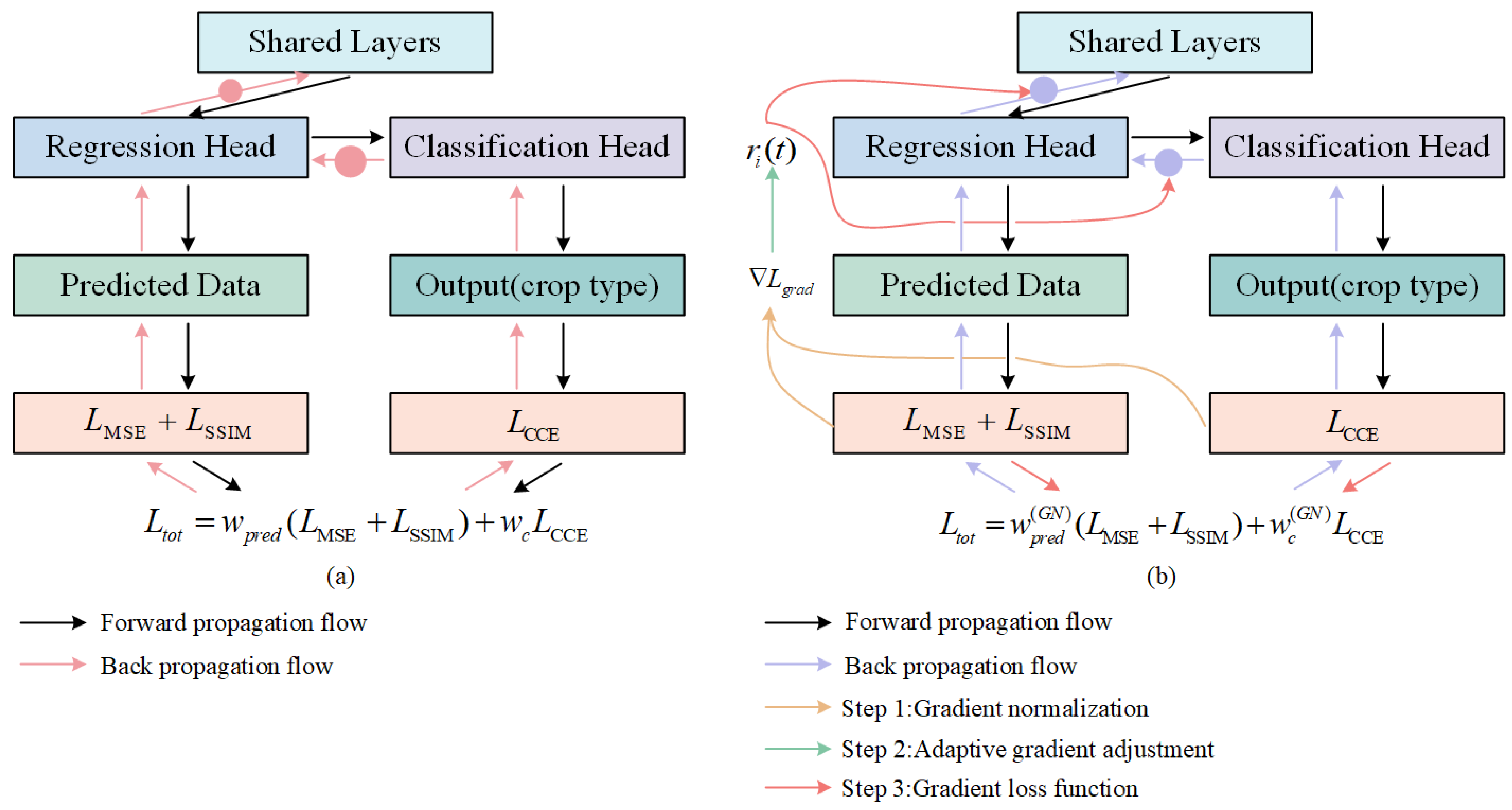
• A cascade learning model is designed, and we enhance the model’s ability to handle time-series data by leveraging Attention encoder–decoder LSTM (AtEDLSTM) to capture global features and a 1D Convolutional Neural Network (1D-CNN) to capture local features. Furthermore, the GradNorm loss weighting method is introduced to balance the learning process of each task to prevent any single task from dominating the optimization process.
• In experiments for early-season classification of soybean, corn and rice in Northeast China, the proposed CLEC framework demonstrates superior classification accuracy and advances the earliest identifiable timing by 10–30 days compared to five state-of-the-art models.

2. Study Area and Data

2.1. Study Area

As shown in Figure 1, the study area of this study is located in the northeastern region of China, covering Heilongjiang Province, Jilin Province and Liaoning Province (39°N–54°N, 115°E–135°E). The region covers a total area of about 0.78 million square kilometers. The northeastern region features diverse topography, including important mountains and plains. The topography gradually rises from west to east, resulting in unique climatic and ecological characteristics.

The region features a temperate monsoon climate with four distinct seasons. Winters are cold and long, while summers are short, warm and humid. The average annual temperature ranges from −5 °C to 10 °C, with precipitation primarily concentrated in the summer. The climatic conditions in this region have a significant impact on crop growth, particularly due to the short growing season, which leads to a more concentrated growth process. The main crops include corn, soybean and rice, which dominate local agricultural production in this region.

The sowing and harvesting calendar of the three main crops in Northeast China is shown in Figure 2 [35], which divides the entire growth stage into three periods: early (DOY: 110–180), mid (DOY: 190–240) and late (DOY: 250–280) [13].

2.2. Data Collection

2.2.1. Satellite Data

This study uses multi-source satellite imagery collected from multiple satellite platforms, including Landsat-7/8, Sentinel-1, Sentinel-2 and MODIS LST. These data provide optical, radar and thermodynamic data for early-season crop classification, covering the data with different temporal and spatial resolutions and offering high timeliness and accuracy [36].

Specifically, Landsat-7/8 and Sentinel-2 serve as optical data sources, effectively monitoring crop growth through multiple bands [37]. Various vegetation indices (VIs) were derived from top-of-atmosphere (TOA) reflectance. Although the temporal sensitivity of TOA reflectance to atmospheric composition imposes limitations on their application, it remains effective at capturing spectral differences between crop types, which are essential for accurate crop classification [38,39]. Furthermore, Sentinel-1 synthetic aperture radar (SAR) data were fused in this study. With its high spatial and temporal resolution, Sentinel-1 demonstrates significant advantages in crop classification and growth monitoring over large agricultural areas [40]. During the early stages of crop classification, optical and radar data complement each other. By integrating these two data sources, we can conduct more comprehensive and accurate crop identification under various weather and environmental conditions [41]. As shown in

Table 1. Characteristics of Landsat 7 and Landsat 8 imagery data.

Bands	Wavelength (μm)		Resolution (m)
	Landsat 7	Landsat 8
Blue	0.45–0.52	0.45–0.51	30
Green	0.52–0.60	0.53–0.59	30
Red	0.63–0.69	0.64–0.67	30
NIR	0.77–0.90	0.85–0.88	30
SWIR1	1.55–1.75	1.57–1.65	30

and

Table 2. Characteristics of Sentinel-2 imagery data.

Bands	Wavelength (μm)		Resolution (m)
	Sentinel-2A	Sentinel-2B
Blue	0.49	0.49	10
Green	0.56	0.56	10
Red	0.66	0.67	10
NIR	0.84	0.83	10
SWIR1	1.61	1.61	20

, for data selection, this study used five fundamental bands from optical data: blue, green, red, near-infrared and shortwave infrared. Additionally, the VV and VH polarization bands from radar data were also included. Surface temperature data from MODIS LST imagery products were used in this study to provide strong support for thermodynamic analyses of crop growth processes [42]. By integrating data from Landsat, Sentinel-2, Sentinel-1 and MODIS LST, multi-source satellite imagery was constructed to characterize crop growth dynamics more accurately.

2.2.2. Field Survey Data

The field survey data for this study were collected from each sample using GIS devices, which recorded the spatial location and land cover type. To ensure the accuracy of the data, all samples were visually verified using high-resolution imagery from Google Earth Engine, eliminating obviously erroneous samples. Samples representing multiple land cover types were collected, covering areas such as rice, corn, soybean, wheat, grasslands, wetlands, forests, water bodies and built-up areas. Of these, a total of 17,870 samples were collected, and the sample distribution is shown in Figure 3. In the experiment, the sample data were divided into three sets, training, validation and testing, in an 8:1:1 ratio.

2.3. Spectrum Data Processing

The fundamental spectral bands were used to compute various spectral indices, including the Normalized Difference Vegetation Index (NDVI), Enhanced Vegetation Index (EVI), Green Canopy Vegetation Index (GCVI), Land Surface Water Index (LSWI) and Radar Vegetation Index (RVI).

NDVI usually reflects the vegetation growth status [43], the vegetation cover, which is expressed by (1):

$$\mathrm{N}\mathrm{D}\mathrm{V}\mathrm{I}={\displaystyle \frac{\mathrm{N}\mathrm{I}\mathrm{R}-\mathrm{R}\mathrm{e}\mathrm{d}}{\mathrm{N}\mathrm{I}\mathrm{R}+\mathrm{R}\mathrm{e}\mathrm{d}}}$$

(1)

where Red is the TOA reflectance value in the red band and NIR is the TOA reflectance value in the near-infrared band.

EVI is usually related to vegetation condition, canopy structure [44], which is expressed by (2):

$$\mathrm{E}\mathrm{V}\mathrm{I}=2.5\times {\displaystyle \frac{\mathrm{N}\mathrm{I}\mathrm{R}-\mathrm{R}\mathrm{e}\mathrm{d}}{\mathrm{N}\mathrm{I}\mathrm{R}+6\times \mathrm{R}\mathrm{e}\mathrm{d}-7.5\times \mathrm{B}\mathrm{l}\mathrm{u}\mathrm{e}+1}}$$

(2)

where Blue is the TOA reflectance value for the blue band.

GCVI usually reflects the green leaf condition of the vegetation, the chlorophyll content [45], which is expressed by (3):

$$\mathrm{G}\mathrm{C}\mathrm{V}\mathrm{I}={\displaystyle \frac{\mathrm{N}\mathrm{I}\mathrm{R}}{\mathrm{G}\mathrm{r}\mathrm{e}\mathrm{e}\mathrm{n}}}-1$$

(3)

where Green is the TOA reflectance value in the green band.

LSWI usually reflects the moisture status of vegetation and soil [46], which is expressed by (4):

$$\mathrm{L}\mathrm{S}\mathrm{W}\mathrm{I}={\displaystyle \frac{\mathrm{N}\mathrm{I}\mathrm{R}-\mathrm{S}\mathrm{W}\mathrm{I}\mathrm{R}}{\mathrm{N}\mathrm{I}\mathrm{R}+\mathrm{S}\mathrm{W}\mathrm{I}\mathrm{R}}}$$

(4)

where SWIR is the TOA reflectance in the shortwave infrared band, and in the case of multispectral imagery (MSI) data, the reflectance in the SWIR1 band.

RVI provides further information on the health of the vegetation [47], which is expressed by (5):

$$\mathrm{R}\mathrm{V}\mathrm{I}={\displaystyle \frac{\mathrm{N}\mathrm{I}\mathrm{R}}{\mathrm{R}\mathrm{e}\mathrm{d}}}$$

(5)

3. Methodology

3.1. The Overview of the CLEC Framework

As shown in Figure 4, CLEC consists of two main components: data preprocessing and a cascade learning model.

Specifically, this study uses time-series data collected from multiple satellite platforms. First, different data sources undergo preprocessing independently, including denoising with the Refined LEE filter, quality filtering, cloud and snow masking and spectral band normalization. Field survey is conducted to collect ground truth data for calibration and validation. Next, VV, VH and LST are obtained, along with five base bands and various vegetation indices. Ten-day time-series data are constructed by synthesizing the maximum value of GCVI every ten days to retain key growth information. Finally, linear interpolation is applied to ensure data consistency and completeness. After preprocessing, the data are inputted into the cascade learning model.

The cascade learning model includes two different types of deep learning modules: AtEDLSTM and 1D-CNN. AtEDLSTM is used to predict data. The predicted data are then concatenated with early-season time-series data to form full-year time-series data before being inputted into the 1D-CNN. The 1D-CNN extracts sufficient features for crop classification based on the full-year time-series data, thus improving classification accuracy. Meanwhile, the classification and prediction results are optimized jointly through the prediction and classification loss functions, thereby enhancing the performance of the cascade learning model.

3.2. Cascade Learning Model

As shown in Figure 4, the cascade learning model consists of a data prediction module and a crop classification module. Specifically, AtEDLSTM effectively models the complex temporal relationships in the time-series data globally. Meanwhile, 1D-CNN extracts local features from the time-series data for crop classification. By integrating these two different modules, the cascade learning model can better capture both global and local features in the time-series data, resulting in improved classification performance.

3.2.1. AtEDLSTM

Existing prediction models typically rely on hidden-state recurrent propagation or global self-attention mechanisms, which struggle to effectively globally model time-series data when available data are scarce. AtEDLSTM is built upon LSTM and incorporates an encoder–decoder structure combined with an additive attention mechanism. This design overcomes the limitation of conventional LSTM models that rely solely on the final hidden state to enable a more comprehensive representation of temporal dynamics. Meanwhile, in contrast to Transformer-based methods, it achieves effective performance without requiring large-scale training data. AtEDLSTM progressively decodes future data and dynamically focuses on relevant input features.

In addition, AtEDLSTM is fundamentally different from traditional spatiotemporal data fusion models [48,49]. Spatiotemporal fusion methods are typically applied in preprocessing to generate satellite imagery with both high temporal and high spatial resolution. Although these methods can effectively gap-fill the available observations, they are restricted to interpolation within the observed period. In contrast, AtEDLSTM utilizes preprocessed existing observational data to predict future data in order to supplement critical phenological information of crops.

As shown in Figure 5b, in AtEDLSTM, the forgetting gate $f_t$ decides to discard historical information, which can be expressed by (6):

$$f_t=\sigma \left(W_f\cdot \left[h_{t-1},x_t\right]+b_f\right)$$

(6)

where $f_t$ is the output of the forgetting gate. $\sigma$ is the sigmoid activation function. $h_{t-1}$ is the hidden state of the previous moment. $x_t$ is the input of the current moment. ${W_f, b}_{f }$ are the learnable parameters of the model.

The input gate $i_t$ controls the input of new information, which can be expressed by (7):

$$i_t=\sigma \left(W_i\cdot \left[h_{t-1},x_t\right]+b_i\right)$$

(7)

where $i_t$ is the output of the input gate. ${W_i, b}_i$ are the learnable parameters of the model.

The candidate cell state ${\tilde{C}}_t$ updates the cell state $C_t$, which can be expressed by (8) and (9):

$$\widetilde{C_t}=\tanh \left(W_c\cdot \left[h_{t-1},x_t\right]+b_c\right)$$

(8)

$$C_t=f_t\cdot C_{t-1}+i_t\cdot {\tilde{C}}_t$$

(9)

where ${\tilde{C}}_t$ is the value of the candidate memory unit. $C_t$ is the state of the memory unit at the current moment. $C_{t-1}$ is the state of the memory unit at the previous moment. $f_t\cdot C_{t-1}$ is the memory of the forgetting part. $i_t\cdot {\tilde{C}}_t$ is the updating of the input part. $W_c, b_c$ are the learnable parameters of the model.

The output gate $o_t$ decides which information to pass to the current hidden state $h_t$, which can be expressed by (10) and (11):

$$h_t=o_t\cdot \tanh \left(C_t\right)$$

(10)

$$o_t=\sigma \left(W_o\cdot \left[h_{t-1},x_t\right]+b_o\right)$$

(11)

where $h_t$ is the hidden state at the current moment. $o_t$ is the output of the output gate. $W_o,{ b}_{o }$ are the learnable parameters of the model.

Additive attention: The additive attention mechanism reflects the importance of time-series data from various periods by dynamically assigning weights to different time steps [50]. Furthermore, the additive attention mechanism uses activation functions to handle these nonlinear and complex time-series data features to enhance the model’s expressive capability.

The decoder’s hidden state and the encoder’s output sequence are transformed into three components: query, key and value. The query and key are then used to compute the attention weights, which correspond to the importance of each hidden feature at different time steps to the final output. The attention weights are then used to weight the values in the time-series data, with these weights obtained from the output of the attention layer (Figure 5a). The way the additive attention mechanism works can be expressed by (12):

$$Attention\left(Q,K,V\right)=\mathrm{S}\mathrm{o}\mathrm{f}\mathrm{t}\mathrm{m}\mathrm{a}\mathrm{x}\left(W_a\cdot \tanh \left(W_{q}Q+W_{k}K\right)\right)\cdot V$$

(12)

where Q, K and V denote query, key and value, respectively. $W_Q,{ W}_K \mathrm{a}\mathrm{n}\mathrm{d} W_v$ are learnable parameters.

LSTM-based encoder–decoder: The encoder–decoder structure can capture the complex mapping relationship between the input and output through the intermediate hidden states. This enables it to effectively handle complex nonlinear time-series data. Therefore, this study constructs an encoder–decoder structure based on LSTM (Figure 5a).

The encoder understands the initial input through different LSTM cells and summarizes important information to provide input for the subsequent network layers. As shown in Figure 5a, the decoder receives two key inputs in each round of processing. The first is the encoded representation $H_{enc}$ of the entire input sequence obtained by the attention mechanism, which focuses on the information most relevant to the current prediction. The second is the predicted value from the previous time step, which helps to establish a sequential understanding of the time-series data.

3.2.2. D-CNN

As shown in Figure 6, 1D-CNN consists of three Conv1d convolution blocks. Time-series data $X\in R^{B\times D\times T}$ (where $B$ is the batch size, $T$ is the length of the input sequence and $D$ is the dimensionality of the input features) are inputted into the Conv1d convolutional blocks. Each convolutional block contains a Conv1d layer and a ReLU activation layer, which can be expressed by (13) and (14):

$$Z_l=\mathrm{C}\mathrm{o}\mathrm{n}\mathrm{v}1\mathrm{d}\left(X_{l-1},W_l\right)+b_l$$

(13)

$$A_l=\mathrm{R}\mathrm{e}\mathrm{L}\mathrm{U}\left(Z_l\right)$$

(14)

where ${ Z}_l$ is the output of the convolution operation. $X_{l-1}$ is the output of layer $l-1$ (for the first layer, the input is the original data, represented by $X$). $W_l$ is the convolution kernel of the $l$-th layer. $b_{l }$ is the bias term, and $A_l$ is the output of the ReLU layer. The kernel sizes differ across the layers, with values of 128, 64 and 32, respectively.

After the convolution operation in the second and third layers, we apply the Maxpool layer to reduce the size of the feature map. The Maxpool layer uses a 2 × 2 pooling window to down sample features at each time step, thus reducing the computation and retaining the most important features. For the Maxpool operation at the $l$-th layer, the pooling can be expressed by (15):

$$P_l=\mathrm{M}\mathrm{a}\mathrm{x}\mathrm{p}\mathrm{o}\mathrm{o}\mathrm{l}\left(A_l\right)$$

(15)

Through three layers of convolution and pooling operations, the model progressively extracts hierarchical features from the data. As the network depth increases, it captures increasingly complex patterns.

3.3. Loss Function

3.3.1. Prediction and Classification Loss Functions

Prediction loss function: This study combines Mean Squared Error (MSE) with the Structural Similarity Index (SSIM), which can be expressed by (16). SSIM evaluates the structural similarity between the predicted and actual time-series data [51]. When combined with Mean Squared Error (MSE), it can reduce overall error while precisely capturing key change points.

$$L_{pred}=\mathrm{M}\mathrm{S}\mathrm{E}\left(h\left(x\right),y\right)+\left(1-\mathrm{S}\mathrm{S}\mathrm{I}\mathrm{M}\left(h\left(x\right),y\right)\right)$$

(16)

where $h\left(x\right)$ represents the predicted time-series data from the prediction task. $y$ represents the real data.

Classification loss function: this study uses Categorical Cross-Entropy (CCE), which can be expressed by (17):

$$L_c=\mathrm{C}\mathrm{C}\mathrm{E}\left(\widehat{z},z\right)$$

(17)

where $\widehat{z }$ is the actual crop labels. $z$ represents the classification results from the classification task.

3.3.2. Multi-Task Loss Weighting Approach

The traditional multi-task loss weighting method assigns weights to different task loss functions by manually setting weighting coefficients $w_i$, which can be expressed by (18). However, due to the different learning rates of different tasks, certain tasks may dominate the back propagation. This may lead to over-optimization of certain objectives, neglecting the learning of other objectives (Figure 7a). To address this issue, we use the GradNorm [52], which dynamically adjusts the loss weights of different tasks to maintain balanced training of the model (Figure 7b).

$$L=\sum _i{w}_i{L}_i$$

(18)

As shown in Figure 7b, its main steps include the following three parts:

Step 1: Gradient normalization. GradNorm normalizes the gradients of different tasks to a common scale by calculating the gradient $L_2$norm for each task.

For the task $i$ gradient norm, it can be calculated as follows:

$$G_W^{\left(i\right)}\left(t\right)={‖{\nabla }_w{W}_i\left(t\right)L_i\left(t\right)‖}_2$$

(19)

where ${ G}_W^{\left(i\right)}\left(t\right)$ is the gradient paradigm of the $i$-th task at the $t$-th epoch. ${\nabla }_w$ is the derivation of the model parameter $W$. $W_i\left(t\right)$ is the weight of task $i$. $L_i\left(t\right)$ is the loss of the $i$-th task at the $t$-th epoch.

Then, the average gradient parameter of all tasks is calculated as the benchmark of the shared scale:

$${\overline{G}}_W\left(t\right)=E_{task}\left[G_W^{\left(i\right)}\left(t\right)\right]$$

(20)

where ${\overline{G}}_W\left(t\right)$ is the average gradient paradigm of all tasks. $E_{task}$ is the average value of this metric for each task.

Step 2: Adaptive gradient adjustment. By adjusting the magnitude of back propagation gradient for each task, the training rates of the tasks are balanced relative to each other.

The training rate of each task can be calculated as follows:

$${\tilde{L}}_i={\displaystyle \frac{L_i\left(t\right)}{L_i\left(0\right)}},r_i\left(t\right)={\displaystyle \frac{{\tilde{L}}_i\left(t\right)}{E_{task}\left[{\tilde{L}}_i\left(t\right)\right]}}$$

(21)

where ${\widetilde{ L}}_i\left(t\right)$ is the ratio of the loss of task $i$at the$t$-th epoch to the initial loss. $L_i\left(0\right)$ is the loss value of the task at the initial moment. ${ r}_i\left(t\right)$ is the relative training rate of the task.

The target gradient parameter for task $i$ can be defined as follows:

$$G_W^{\left(i\right)}\left(t\right)\mapsto {\overline{G}}_W\left(t\right)\times {\left[r_i\left(t\right)\right]}^a$$

(22)

where ${ \left[r_i\left(t\right)\right]}^a$ is used to dynamically adjust the target gradient of the task $i$. $a$ is the super parameter, indicating the adjustment strength of the task learning speed; the larger $a$ is, the greater the adjustment strength.

Step 3: Gradient loss function. To implement gradient adjustment, GradNorm introduces a gradient loss function $L_{grad}$. As shown in (23), the gradient loss is calculated using $L_1$ norm, evaluating the loss between the output and target values for each task. Finally, the losses from all tasks are summed to obtain the total gradient loss.

$$L_{grad}\left(t;w_i\left(t\right)\right)=\sum _i{\left|G_W^{\left(i\right)}\left(t\right)-{\overline{G}}_W\left(t\right)\times {\left[r_i\left(t\right)\right]}^a\right|}_1$$

(23)

4. Experiment and Analysis

4.1. Evaluation Metrics

In this section, comparative experiments and ablation studies are conducted. We selected the F1-score and Kappa as the overall performance metric for all models. The F1-score reflects the balance between precision and recall for specific categories of the method. Kappa reflects the actual classification consistency of the method.

The F1-score can be calculated as in (24)–(26):

$$\mathrm{P}\mathrm{r}\mathrm{e}\mathrm{c}\mathrm{i}\mathrm{s}\mathrm{i}\mathrm{o}\mathrm{n}={\displaystyle \frac{TP}{TP+FP}}$$

(24)

$$\mathrm{R}\mathrm{e}\mathrm{c}\mathrm{a}\mathrm{l}\mathrm{l}={\displaystyle \frac{TP}{TP+FN}}$$

(25)

$$\mathrm{F}1-\mathrm{s}\mathrm{c}\mathrm{o}\mathrm{r}\mathrm{e}={\displaystyle \frac{2\times \mathrm{P}\mathrm{r}\mathrm{e}\mathrm{c}\mathrm{i}\mathrm{s}\mathrm{i}\mathrm{o}\mathrm{n}\times \mathrm{R}\mathrm{e}\mathrm{c}\mathrm{a}\mathrm{l}\mathrm{l}}{\mathrm{P}\mathrm{r}\mathrm{e}\mathrm{c}\mathrm{i}\mathrm{s}\mathrm{i}\mathrm{o}\mathrm{n}+\mathrm{R}\mathrm{e}\mathrm{c}\mathrm{a}\mathrm{l}\mathrm{l}}}$$

(26)

where $TP$, $TN$, $FP$ and $FN$ represent the number of true positives, true negatives, false positives and false negatives, respectively.

Kappa can be calculated as in (27)–(29):

$$P_o={\displaystyle \frac{1}{N}}\sum _{i=1}^K{n}_i^{corr}$$

(27)

$$P_e={\displaystyle \frac{1}{N^2}}\sum _{i=1}^K{n}_i^{pred}{n}_i^{true}$$

(28)

$$\mathrm{K}\mathrm{a}\mathrm{p}\mathrm{p}\mathrm{a}={\displaystyle \frac{P_o-P_e}{1-P_e}}$$

(29)

where $P_o$ represents the correctness of the observation, calculated by summing the number of correctly categorized samples in each category $n_i^{corr}$and dividing by the total number of samples $N$. $P_e$ represents the expected correctness in the stochastic case, calculated by summing the product of the number of samples in each category for the predicted values${ n}_i^{pred}$ and true values $n_i^{true}$and dividing by the square of the total number of samples.

4.2. Comparison Experiment

4.2.1. Experimental Design

To demonstrate the superiority of the developed CLEC in early-season crop classification, we constructed rice and non-rice classification, corn and non-corn classification and soybean and non-soybean classification for comparative evaluation.

In the comparative evaluation, we selected the four different state-of-the-art (SOTA) models (RF, SVM, DeepCropMapping and Transformer) to compare with CLEC. RF was configured with 500 trees, and its maximum feature count was set to the square root of the input features. SVM employed an RBF kernel with a regularization parameter C of 3. To ensure experimental consistency, both DeepCropMapping (DCM) and Transformer adopted the same classification loss function, learning rate and optimizer as those utilized in the deep learning component of the CLEC framework.

4.2.2. Comparison with Other Methods

As shown in

Table 3. Comparison of performance of CLEC with methods for early-season classification of soybean.

Method	Day of Year
	140	150	160	170	180	190	200	210	220	230
Transformer	0.445	0.484	0.515	0.540	0.622	0.703	0.808	0.852	0.861	0.842
DCM	0.472	0.461	0.498	0.519	0.587	0.717	0.821	0.856	0.865	0.854
RF	0.470	0.473	0.512	0.539	0.589	0.695	0.765	0.824	0.850	0.847
SVM	0.000	0.004	0.032	0.063	0.142	0.317	0.594	0.741	0.798	0.792
CLEC	0.516	0.551	0.580	0.576	0.657	0.755	0.819	0.845	0.866	0.853

, during the crop growth stage from soybean sowing to the pod-setting stage (DOY: 140–230), CLEC performs most prominently from the sowing to the third true leaf stage (DOY: 140–190). CLEC’s Kappa at each time point is significantly higher than that of the other methods. Compared to RF, Transformer and DCM, CLEC achieves an average improvement of 6.0%, 5.4% and 6.4%, respectively. Over time, DCM achieves the best results at some of the mid-term time points (DOY: 200–230), while CLEC slightly outperforms DCM at some of the time points. In the overall classification performance during the early growth stage of soybean, CLEC shows good classification performance.

As shown in

Table 4. Comparison of performance of CLEC with methods for early-season classification of corn.

Method	Day of Year
	140	150	160	170	180	190	200	210	220	230
Transformer	0.487	0.486	0.514	0.525	0.607	0.684	0.774	0.811	0.822	0.817
DCM	0.492	0.500	0.528	0.542	0.579	0.675	0.764	0.809	0.808	0.833
RF	0.457	0.479	0.478	0.473	0.533	0.664	0.756	0.792	0.813	0.824
SVM	0.096	0.138	0.126	0.153	0.233	0.482	0.629	0.694	0.723	0.747
CLEC	0.540	0.556	0.552	0.577	0.633	0.717	0.780	0.819	0.843	0.864

, during the growth phase of corn from sowing to the heading stage (DOY: 140–230), CLEC achieves the highest classification Kappa at each time point, outperforming all other methods. Specifically, CLEC performs best from the sowing to the stem elongation stage (DOY: 140–190), with an average improvement of 8.2%, 4.5% and 4.3% compared to RF, Transformer and DCM, respectively. CLEC outperforms the suboptimal comparator by 0.6% to 3.1% at various times in the corn mid-growth season (DOY: 200–230).

As shown in

Table 5. Comparison of performance of CLEC with methods for early-season classification of rice.

Method	Day of Year
	80	90	100	110	120	130	140	150	160	170
Transformer	0.393	0.562	0.631	0.717	0.768	0.836	0.912	0.939	0.933	0.934
DCM	0.498	0.578	0.584	0.666	0.734	0.830	0.924	0.937	0.944	0.944
RF	0.386	0.424	0.455	0.576	0.690	0.787	0.892	0.921	0.933	0.933
SVM	0.000	0.000	0.000	0.000	0.384	0.666	0.865	0.921	0.919	0.926
CLEC	0.577	0.634	0.650	0.746	0.770	0.871	0.925	0.940	0.947	0.947

, during the growth phase of rice from 30 days before sowing to the tillering stage (DOY: 80–170), CLEC achieves the highest Kappa at each time point, outperforming all other methods. Specifically, CLEC performs best in the stage from 30 days before sowing to the seeding/flooding stage (DOY: 80–130), with an average improvement of 15.5%, 5.7% and 6% compared to RF, Transformer and DCM, respectively. In the transplanting-to-tillering stage of rice growth (DOY: 140–170), CLEC outperforms the next-best comparison models with a slight advantage at various time points.

As shown in Table 3, Table 4 and Table 5, in the comparative experiments, when the crops enter the mid-growth stage (e.g., corn and soybean: DOY: 200–230), the crop phenological information gradually increases. With the accumulation of information, CLEC and baseline models have acquired sufficient crop growth features. The classification models are able to better identify the phenological differences between the crops, and thus the classification accuracy tends to saturate.

However, when the classification time is earlier, CLEC significantly outperforms the other baseline models at classification. This is mainly attributed to CLEC solving the problem of insufficient extraction of critical phenological information through the cascade learning mechanism, leading to a significant improvement in classification accuracy compared to the baseline models.

4.2.3. Earliest Identifiable Timing

In Figure 8, with the increase in temporal information throughout the crop growth process, the variation in F1-score for crop classification at different time points using different methods is shown. The earliest identifiable timing (F1-score > 0.8) is marked with purple, orange, blue, red and green shading. Figure 9 shows the comparison of the crop classification results at the earliest identifiable timing between deep-learning-based methods across subregions.

As shown in Figure 8a,b,e,f, the earliest identifiable timing for CLEC in soybean and rice occurs at DOY 190 and DOY 120, respectively, which is 10 days earlier than Transformer, DCM and RF (i.e., DOY 200 and DOY 130), and 30 days and 20 days earlier than SVM (i.e., DOY 220 and DOY 140, respectively). Figure 8c,d show that for corn, CLEC, RF, Transformer and DCM reach the earliest identifiable timing simultaneously, but the F1-score of CLEC is slightly higher than that of the other three models. Compared to SVM, CLEC reaches the earliest identifiable timing 30 days earlier. As shown in Figure 9, CLEC exhibited the best agreement with the actual cropland boundaries and produced less misclassification noise for soybean and corn in the subregion. In contrast, both DCM and Transformer show minor misclassifications. For rice, as some fields had already entered the flooding stage, making them relatively easier to distinguish, all three models perform comparably within the subregion.

These excellent results indicate that CLEC, with its cascade learning mechanism, is able to extract more critical phenological information, thus demonstrating a significant advantage in early-season crop classification.

4.3. Ablation Experiments in CLEC

To evaluate the effectiveness of the cascade learning mechanism, the encoder–decoder structure, the attention mechanism and the loss function, we conducted ablation experiments on CLEC. A 1D-CNN was used as a baseline model to evaluate the effectiveness of cascade learning. We compared CLEC with CLEC_NoAtED to verify the effectiveness of the encoder–decoder structure and the attention mechanism. Additionally, we compared CLEC with CLEC_NoGrad to demonstrate the effectiveness of GradNorm in the model.

As shown in

Table 6. Comparison of ablation experiment performance of CLEC for early-season classification of soybean.

Method	Attention	Loss Function				Day of Year
		CCE	MSE	SSIM	Grad	140	150	160	170	180	190	200	210	220	230
1DCNN		√				0.469	0.505	0.546	0.525	0.593	0.692	0.807	0.835	0.852	0.851
CLEC_NoAtED		√	√			0.502	0.526	0.559	0.566	0.641	0.742	0.805	0.850	0.861	0.852
CLEC_NoGrad	√	√	√	√		0.507	0.565	0.540	0.583	0.653	0.750	0.807	0.851	0.873	0.852
CLEC	√	√	√	√	√	0.516	0.551	0.580	0.576	0.657	0.755	0.819	0.845	0.866	0.853

,

Table 7. Comparison of ablation experiment performance of CLEC for early-season classification of corn.

Method	Attention	Loss Function				Day of Year
		CCE	MSE	SSIM	Grad	140	150	160	170	180	190	200	210	220	230
1DCNN		√				0.442	0.471	0.499	0.498	0.537	0.682	0.776	0.804	0.817	0.840
CLEC_NoAtED		√	√			0.526	0.537	0.570	0.572	0.622	0.702	0.793	0.818	0.820	0.842
CLEC_NoGrad	√	√	√	√		0.536	0.558	0.562	0.609	0.643	0.699	0.793	0.815	0.834	0.844
CLEC	√	√	√	√	√	0.540	0.556	0.552	0.577	0.633	0.717	0.780	0.819	0.843	0.864

and

Table 8. Comparison of ablation experiment performance of CLEC for early-season classification of rice.

Method	Attention	Loss Function				Day of Year
		CCE	MSE	SSIM	Grad	80	90	100	110	120	130	140	150	160	170
1DCNN		√				0.375	0.489	0.559	0.668	0.709	0.814	0.907	0.932	0.934	0.931
CLEC_NoAtED		√	√			0.535	0.602	0.672	0.706	0.756	0.856	0.924	0.944	0.944	0.951
CLEC_NoGrad	√	√	√	√		0.526	0.606	0.665	0.689	0.763	0.864	0.922	0.934	0.944	0.955
CLEC	√	√	√	√	√	0.577	0.634	0.650	0.746	0.770	0.871	0.925	0.940	0.947	0.947

, compared to the baseline model 1D-CNN, the three frameworks using cascade learning all demonstrate better classification performance, proving the effectiveness of cascade learning. At most time points, CLEC outperforms CLEC_NoAtED. Specifically, CLEC achieved the best Kappa at various time points for soybean, corn and rice classifications, with average improvements of 1.1%, 0.8% and 1.2%, respectively. Although CLEC slightly underperforms compared to CLEC_NoGrad at certain time points for corn classification, CLEC generally performs better than CLEC_NoGrad in soybean and rice classifications and achieves the best Kappa classification results.

The experimental results demonstrate that each module exhibits a certain degree of effectiveness. By integrating the advantages of each module, CLEC achieves superior performance in early-season crop classification.

5. Discussion

5.1. Relationship Between Classification Performance and Phenological Stages

This study proposes CLEC for early-season crop classification, which includes the cascade learning model that simultaneously performs data prediction and crop classification tasks, aiming to address the issue of extracting insufficient critical phenological information. The experimental results show that compared to baseline models, CLEC demonstrates superior classification accuracy and earlier identification capability.

Existing methods have primarily focused on improving feature extraction and fusion capabilities. Xu et al. [25] proposed DeepCropMapping (DCM), which utilizes the AtBiLSTM module to perform crop classification. Weilandt et al. [23] employed a temporal attention encoder to enhance data feature extraction. These methods utilize limited early data for classification without supplementing future crop growth information. As a result, when available data are scarce, these methods struggle to capture sufficient critical phenological information. In contrast, CLEC incorporates an additional prediction module, which is based on LSTM. This module is used to supplement the classification module with more data. Moreover, CLEC leverages the cascade learning mechanism to iteratively optimize both prediction and classification results.

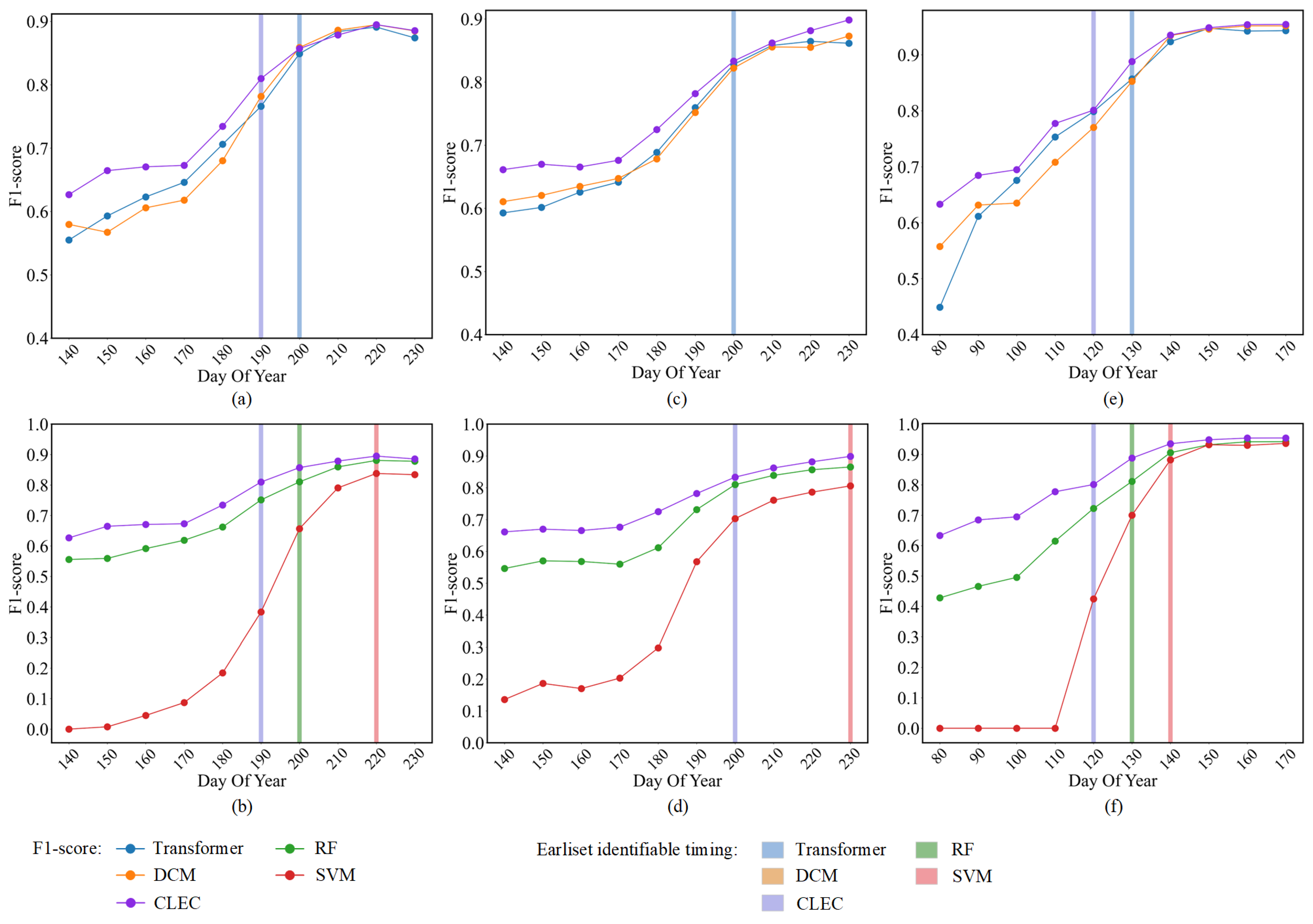
In the early stages of crop growth (DOY 110–180), CLEC achieved F1-scores of 62.7–71.4% for soybean, 66.1–72.5% for corn and 63.3–95.5% for rice. Specifically, rice reached its earliest identifiable timing at the beginning of the flooding stage (DOY 120). This is primarily due to the relatively high LSWI values of rice during the flooding/transplanting stage (DOY 120–150), which serve as a key feature for distinguishing rice from corn and soybean. Therefore, this phenological characteristic plays a crucial role in rice classification. Meanwhile, although the classification accuracy of soybean and corn has not yet reached the earliest identifiable timing (F1-score > 0.8), it still significantly outperforms other models in the comparative experiments.

In the mid-growth stage of crops (DOY 190–240), soybean and corn enter a vigorous growth stage, with gradually increasing vegetation cover. In this stage, vegetation indices play a crucial role in crop identification, with soybean reaching its earliest identifiable timing at the third true leaf stage (DOY 190) and corn at the stem elongation stage (DOY 200).

As crops enter the mid-to-late growth stages, the time-series data accumulate sufficient critical phenological information, leading to a gradual saturation of classification accuracy. At this stage, further increasing the time-series length results in only a slow improvement in accuracy.

The above conclusion is generally consistent with other studies [13,53,54]. Regarding the earliest identifiable timing of crops, the results obtained by CLEC are reliable and achieve an earlier identification compared to other studies.

5.2. Explanation of the CLEC Advantages in the Early-Season Crop Classification

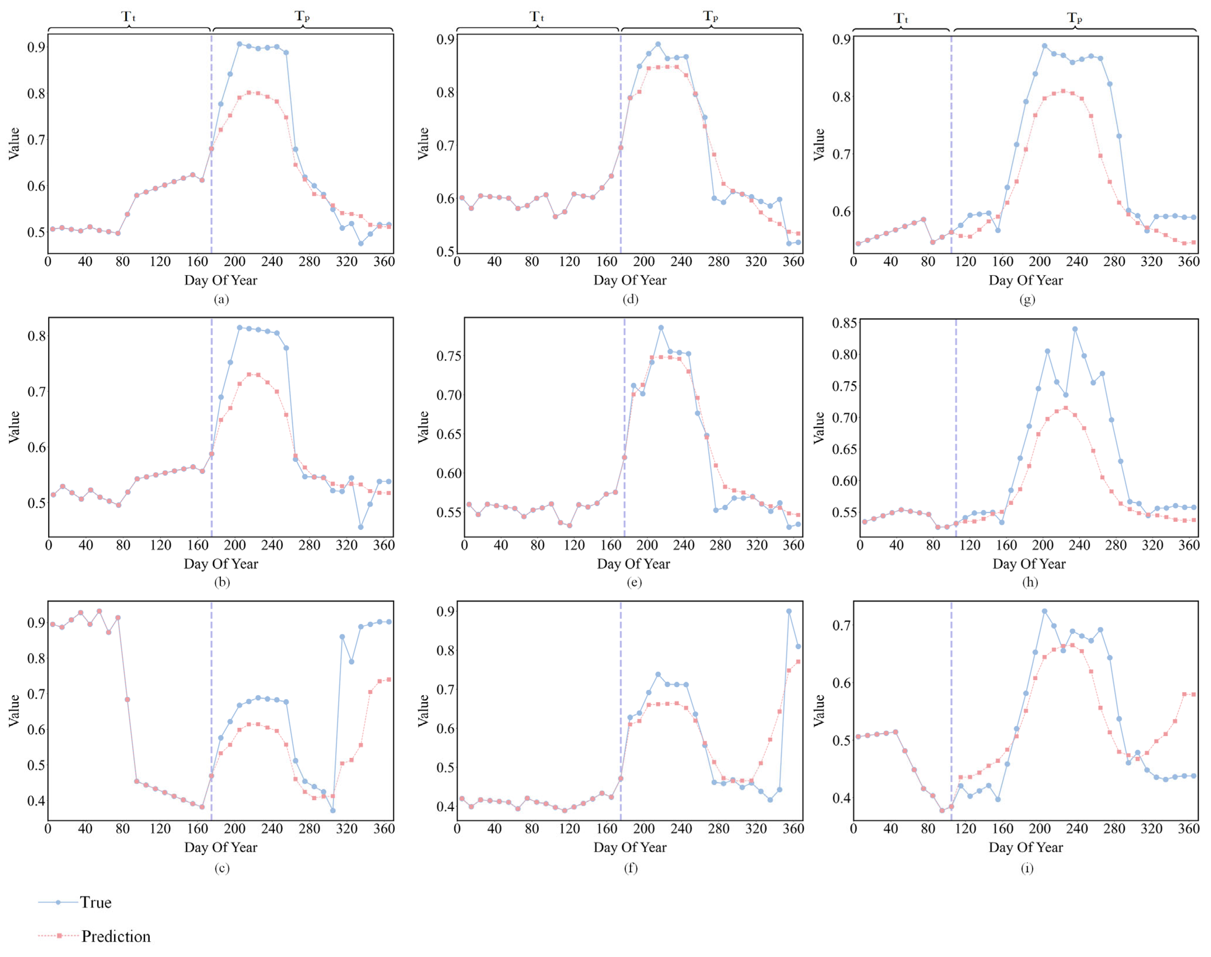
To further analyze the advantages of CLEC in early-season crop classification, we compared the trend variations between the generated data and the real to validate the accuracy of the predictions by AtEDLSTM. We selected three indices, EVI, NDVI and LSWI. EVI reflects changes during periods of high biomass [55], and NDVI is sensitive to changes in green leaf area and biomass [56]. LSWI is very sensitive to changes in leaf and soil moisture and plays a key role in the identification of rice, corn and soybean [57]. Figure 10 shows the comparative results of these three indices.

At DOY 110, rice enters the sowing stage but has not yet entered the flooding/transplanting stage (DOY 120–150), at which point the difference in LSWI between rice and corn and soybean is not significant (Figure 10c,f,i). When this critical phenological information is lacking, the classification model struggles to effectively capture the phenological feature differences between rice and other crops during their growth stage. To address this problem, CLEC uses AtEDLSTM to supplement the time-series data. AtEDLSTM is capable of generating the trend variations of LSWI for rice in the flooding/transplanting stage (DOY 120–150) (Figure 10i). This provides critical phenological information for the 1D-CNN, thereby effectively distinguishing rice from corn and soybean.

At DOY 180, corn enters the stem elongation stage with rapidly elongating stems, while soybean is in the third true leaf stage, when the spectral difference between the two is not significant. As shown in Figure 10a–f, AtEDLSTM is able to predict the key feature variation trends for both crops during the peak growth stage (DOY 200–240), providing more critical information.

However, from the observation of Figure 10, we can see that there is still room for improvement in the prediction performance of AtEDLSTM in CLEC. Currently, it can only predict the general trend of the feature curve (baseline). The learning and prediction of periodic patterns (peaks and valleys) that fluctuate around the baseline due to phenological events (such as planting, heading and harvest) are still not ideal and require further optimization. These localized fluctuations often correspond to critical phenological information and are essential for distinguishing crop types. Under non-standard growing conditions such as drought or late sowing, crop growth trajectories often deviate significantly from typical patterns. Due to the inherently small inter-species differences, particularly between soybean and corn, which exhibit highly similar spectral and phenological curves, these crops are more prone to misclassification. Identifying crops under such non-standard conditions presents two major challenges:

First, compared with historical years, the feature values at the same growth stage under non-standard conditions may fluctuate to some extent. For example, during droughts, the NDVI curve tends to be systematically lower. At the same time, the temporal distribution of growth stages on the calendar may shift, resulting in earlier or later development, or in stretching or compression of the phenological phases. These factors can lead to a significant increase in the prediction error of AtEDLSTM.

Second, since AtEDLSTM has difficulty capturing and predicting finer-grained fluctuations caused by phenological events, 1D-CNN must rely primarily on the overall trend of the feature curves. Under non-standard conditions, this overall trend is already subject to considerable uncertainty. Moreover, the lack of effective modeling of key variation points such as peaks and troughs further limits the model’s capacity to learn from detailed features. This limitation prevents 1D-CNN from leveraging prominent local features for correction, ultimately resulting in a decrease in classification accuracy.

These errors propagate progressively through the cascade learning pipeline, leading to a further decline in overall classification performance.

5.3. The Impact of Prediction Data Length and Prediction Mode on Classification Accuracy

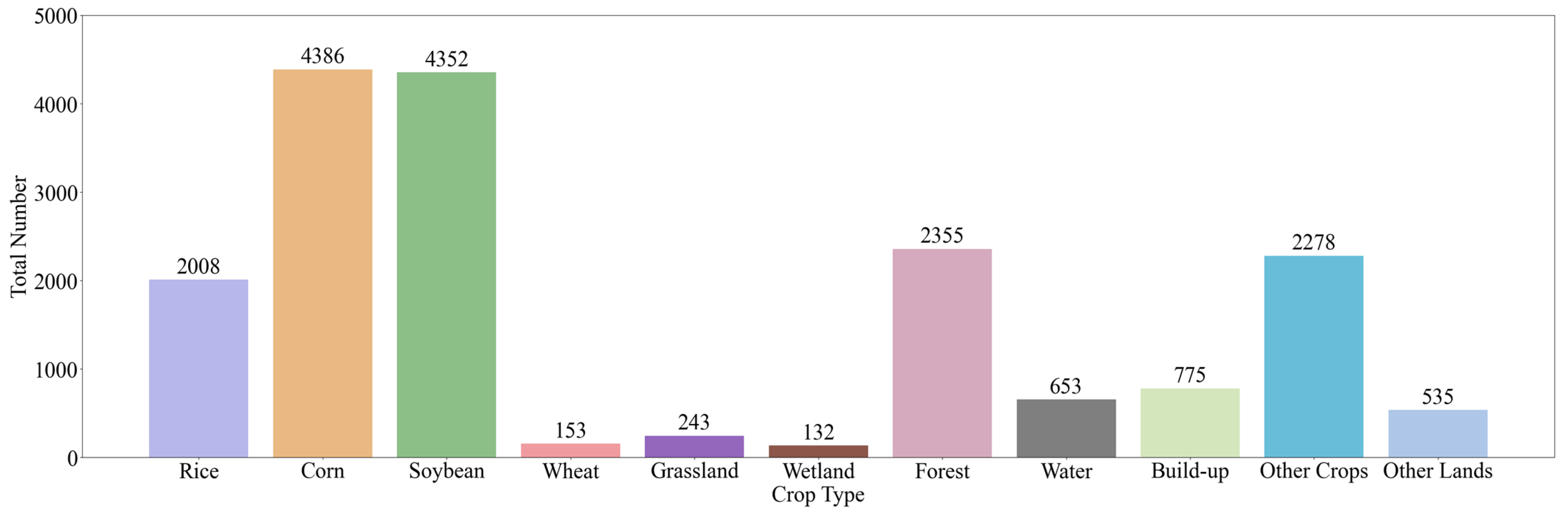
In the cascade learning model, the predicted data are concatenated with early-season time-series data to form the full-year time series. However, as shown in Figure 2, most crops reach their harvest stage between late September and early October (DOY 270–280). In the post-harvest stage (DOY 290–370), fluctuations in time-series data are primarily driven by non-crop growth factors. Therefore, predicting data at this stage may not improve early-season crop classification accuracy and could even negatively impact the classification results.

To investigate the effect of predicted data length on early-season crop classification accuracy in the cascade learning model, we conducted an experiment. For soybean, we used early-season data from the first 190 days of the year (DOY: 0–190) as input in the model for further prediction. For corn, we used data from the first 200 days (DOY: 0–200), and for rice, the first 120 days (DOY: 0–120). These time points represent the earliest identifiable timing for each crop, ensuring that the model captures sufficient phenological information for reliable classification. By adjusting the length of the predicted data, we constructed varying time-series datasets to assess the impact of data length on classification accuracy.

As shown in

Table 9. The classification accuracy of crops with different predicted data lengths.

Predicted Data Length	DOY	Soybean		Predicted Data Length	DOY	Corn		Predicted Data Length	DOY	Rice
		Kappa	F1-Score			Kappa	F1-Score			Kappa	F1-Score
60	250	0.758	0.810	50	250	0.773	0.828	130	250	0.768	0.797
70	260	0.733	0.789	60	260	0.790	0.840	140	260	0.745	0.778
80	270	0.736	0.791	70	270	0.787	0.839	150	270	0.757	0.790
90	280	0.736	0.792	80	280	0.797	0.846	160	280	0.762	0.794
100	290	0.732	0.791	90	290	0.780	0.833	170	290	0.750	0.784
110	300	0.738	0.789	100	300	0.793	0.842	180	300	0.746	0.783
120	310	0.739	0.795	110	310	0.777	0.832	190	310	0.762	0.792
130	320	0.742	0.800	120	320	0.785	0.835	200	320	0.749	0.779
140	330	0.743	0.798	130	330	0.791	0.841	210	330	0.762	0.794
150	340	0.737	0.790	140	340	0.787	0.838	220	340	0.767	0.799
160	350	0.756	0.808	150	350	0.781	0.833	230	350	0.760	0.791
170	360	0.748	0.801	160	360	0.782	0.836	240	360	0.754	0.786
180	370	0.755	0.808	170	370	0.780	0.833	250	370	0.770	0.801

, soybean achieves its highest accuracy with a predicted data length of 60 days (predicted to DOY 250), yielding a 0.3% increase in Kappa and a 0.2% increase in F1-score compared to the full-year data, which are completed through prediction based on early-season data. Corn reaches its optimal accuracy at 80 days (predicted to DOY 280), with the Kappa improving by 1.7% and the F1-score increasing by 1.3% in the same comparison. Although the highest classification accuracy for rice is achieved at the final time point (DOY 370), the second-best accuracy is obtained with a predicted data length of 130 days (predicted to DOY 250), which is only 0.2% lower in Kappa and 0.4% lower in F1-score compared to the optimal values. This, however, results in substantial savings in both time and computational costs.

In summary, the length of the predicted data has a certain impact on the performance of CLEC in early-season crop classification. When the predicted data length is excessively long, the prediction performance may degrade because the model could introduce additional noise, leading to a certain impact on classification accuracy. In contrast, when the predicted data length is too short, the cascade learning model may fail to capture sufficient critical phenological information, which can significantly affect classification accuracy. Therefore, future research could further explore the optimal predicted data length for different crops to enhance the classification performance of CLEC.

In addition to investigating the effect of different prediction lengths, we further explored how different prediction modes (representing different prediction errors) affect the classification performance. Specifically, we evaluated three variants: (1) CLEC, our cascade learning framework, in which the prediction and classification modules are jointly optimized; (2) CLEC_V2, in which the prediction and classification modules are trained separately as two independent models, without cascade learning; and (3) CLEC_V3, our cascade learning framework which derives classification results based on the best prediction error of the AtEDLSTM output.

As shown in Figure 11, CLEC outperforms both CLEC_V2 and CLEC_V3 in early-season crop classification accuracy. Notably, although other modes utilize the prediction module that minimizes prediction error, their classification performance remains suboptimal. This indicates that minimizing prediction errors alone does not necessarily lead to optimal classification performance. These results emphasize the critical role of cascade learning in aligning prediction outputs with classification. The cascade learning mechanism enables the prediction module to predict more discriminative features, even when the predicted data are not perfectly accurate.

5.4. Applicability of CLEC Across Agro-Climatic Zones

To further investigate the performance of CLEC in early-season classification across different climatic zones, we conducted experiments. We employed the dataset from the area near Hollfeld in Bavaria, Germany, which is the dataset used in Rußwurm et al.’s research [26]. The region has a temperate continental climate with distinct seasonal variations. The dataset includes a full-year time series of Sentinel-2 imagery, which contains between 71 (every 5 days) and 147 (every 2.5 days) observations. The dataset consists of seven common crop types: meadow, summer barley, corn, winter wheat, winter barley, clover and triticale. The dataset was split into training, validation and test sets, with a ratio of 8:1:1.

We conducted comparative experiments between CLEC and the baselines used in Section 4.2 and Section 4.3. As shown in Figure 12, CLEC significantly outperformed the other methods during the DOY 100–130 period, which is notably early in the crop growth stage. This highlights the practical value of the CLEC in enabling early and reliable crop classification, potentially offering considerable economic and societal benefits.

When more phenological information was accumulated (DOY 130–200), the classification advantage of CLEC diminished. After the earliest identifiable timing, its accuracy was comparable to or slightly inferior to that of DCM. This may be attributed to the reduced marginal benefit of the prediction module at later growth stages. Additionally, the classification performance in this stage may be affected by differences in region-specific feature patterns, which challenge the model’s generalization across different datasets. During this period, the classification accuracy of all models tended to saturate, which is consistent with the experimental results in Section 4.2.

Overall, CLEC still demonstrates a clear advantage in early-season classification, while also exhibiting promising cross-regional transferability in early-season crop identification.

5.5. Limitations and Future Work

Our experiments show that, in the early-to-mid stages of crop growth, CLEC achieves better classification results, demonstrating a certain advantage. However, there are still some limitations that need to be improved in future studies. As shown in Table 3, Table 4 and Table 5 and Figure 8 and Figure 12, CLEC outperforms the baseline methods when the available data are scarce. However, after reaching the earliest identifiable timing, the framework achieves only marginal improvements over the best-performing baselines or performs comparably.

Additionally, we evaluated the computational complexity of CLEC. As shown in

Table 10. A comparison of the computational complexity analysis of the CLEC with methods.

Method	Param Count (M)	Avg Epoch Training Time (s)
Transformer	10.52	2.41
DCM	8.47	1.83
CNN	0.04	0.62
CLEC_NoGrad	2.38	10.42
CLEC	2.38	20.53

, although CLEC consumes less memory than DCM and Transformer, it requires the longest training time among all methods. CLEC exhibits limitations in computational efficiency due to its more complex structure in the classification process. As shown in Table 10, the use of GradNorm for dynamic multi-task loss balancing significantly contributes to the increased training time of CLEC. This is primarily due to the additional computational steps introduced by GradNorm in each training iteration. These steps include multiple backward passes to compute gradient norms, dynamic adjustment of task loss weights and extra gradient tracking via hooks. These operations result in approximately double the training time compared to a variant without GradNorm (CLEC_NoGrad). When time complexity is not a major constraint, CLEC can effectively achieve high performance in early-season crop classification. Future work could investigate more efficient multi-task optimization strategies to enhance scalability and deployment feasibility.

Future work can be developed in the following two aspects. On the one hand, the cascade learning model of CLEC consists of two independent cascading output backbone modules, which possess strong transferability and allow flexible replacement of certain parts within the model. Based on this characteristic, future work could attempt to replace the models for the prediction and classification tasks with other models, optimizing the performance of both tasks and thus enhancing the overall performance of CLEC. On the other hand, further exploration of adaptive loss weighting methods could be pursued to better achieve the mutual optimization between the two tasks, thereby improving the overall performance and stability of CLEC.

6. Conclusions

This study proposes the Cascade Learning Early Classification (CLEC) framework with data preprocessing and a cascade learning model. It aims to address the issue of insufficient phenological features in the very early stages of crop classification. In the data preprocessing stage, we generated high-quality time-series data by integrating optical, radar and thermodynamic data. Meanwhile, we designed a cascade learning model that simultaneously performs prediction and classification tasks to address the issue of insufficient feature extraction. Both the prediction and classification results were jointly optimized through the cascade learning mechanism. Specifically, the cascade learning model was composed of two components: the AtEDLSTM for capturing global temporal dependencies, and the 1D-CNN for extracting local features from time-series data. Additionally, the GradNorm loss weighting method was introduced to dynamically adjust the contribution of each task during training.

To validate the effectiveness of the proposed CLEC framework, we conducted experiments in Northeast China. The experimental results show that CLEC exhibits significant superiority over the baseline 1D-CNN model in early-season crop classification, with the classification Kappa increasing by an average of 3.4–6.9%. CLEC achieved the highest Kappa values in the early growth stage for soybean, corn and rice, significantly improving the classification accuracy compared to four other models. CLEC was able to achieve the earliest identifiable timing for the crops 10 to 30 days earlier than RF, Transformer, DCM and SVM. Additionally, we also conducted ablation experiments on CLEC, and the results demonstrate the effectiveness of each module.

We further explored the relationship between classification accuracy and the phenological stages of crop growth, as well as the advantages of CLEC in early-season classification. This further demonstrates the reliability of our results, which outperform other studies. Additionally, we investigated the impact of varying predicted data lengths in the cascade learning model on classification accuracy, providing a potential direction for future research. Overall, this study provides new ideas for solving the problem of early-season crop classification and demonstrates the great potential of cascade learning in this area.

References

1. Kebede, E.A.; Abou Ali, H.; Clavelle, T.; Froehlich, H.E.; Gephart, J.A.; Hartman, S.; Herrero, M.; Kerner, H.; Mehta, P.; Nakalembe, C.; et al. Assessing and Addressing the Global State of Food Production Data Scarcity. Nat. Rev. Earth Environ. 2024, 5, 295–311. [Google Scholar] [CrossRef]
2. Cai, Y.; Guan, K.; Peng, J.; Wang, S.; Seifert, C.; Wardlow, B.; Li, Z. A High-Performance and in-Season Classification System of Field-Level Crop Types Using Time-Series Landsat Data and a Machine Learning Approach. Remote Sens. Environ. 2018, 210, 35–47. [Google Scholar] [CrossRef]
3. Lei, L.; Wang, X.; Zhang, L.; Hu, X.; Zhong, Y. CROPUP: Historical Products Are All You Need? An End-to-End Cross-Year Crop Map Updating Framework without the Need for in Situ Samples. Remote Sens. Environ. 2024, 315, 114430. [Google Scholar] [CrossRef]
4. Yang, Z.; Diao, C.; Gao, F. Towards Scalable Within-Season Crop Mapping with Phenology Normalization and Deep Learning. IEEE J. Sel. Top. Appl. Earth Obs. Remote Sens. 2023, 16, 1390–1402. [Google Scholar] [CrossRef]
5. Mohammadi, S.; Belgiu, M.; Stein, A. A Source-Free Unsupervised Domain Adaptation Method for Cross-Regional and Cross-Time Crop Mapping from Satellite Image Time Series. Remote Sens. Environ. 2024, 314, 114385. [Google Scholar] [CrossRef]
6. Benami, E.; Jin, Z.; Carter, M.R.; Ghosh, A.; Hijmans, R.J.; Hobbs, A.; Kenduiywo, B.; Lobell, D.B. Uniting Remote Sensing, Crop Modelling and Economics for Agricultural Risk Management. Nat. Rev. Earth Environ. 2021, 2, 140–159. [Google Scholar] [CrossRef]
7. Xia, T.; He, Z.; Cai, Z.; Wang, C.; Wang, W.; Wang, J.; Hu, Q.; Song, Q. Exploring the Potential of Chinese GF-6 Images for Crop Mapping in Regions with Complex Agricultural Landscapes. Int. J. Appl. Earth Obs. Geoinf. 2022, 107, 102702. [Google Scholar] [CrossRef]
8. Cai, Z.; Xu, B.; Yu, Q.; Zhang, X.; Yang, J.; Wei, H.; Li, S.; Song, Q.; Xiong, H.; Wu, H.; et al. A Cost-Effective and Robust Mapping Method for Diverse Crop Types Using Weakly Supervised Semantic Segmentation with Sparse Point Samples. ISPRS J. Photogramm. Remote Sens. 2024, 218, 260–276. [Google Scholar] [CrossRef]
9. Wen, C.; Lu, M.; Bi, Y.; Xia, L.; Sun, J.; Shi, Y.; Wei, Y.; Wu, W. Customized Crop Feature Construction Using Genetic Programming for Early- and in-Season Crop Mapping. Comput. Electron. Agric. 2025, 231, 109949. [Google Scholar] [CrossRef]
10. Li, H.; Di, L.; Zhang, C.; Lin, L.; Guo, L.; Yu, E.G.; Yang, Z. Automated In-Season Crop-Type Data Layer Mapping Without Ground Truth for the Conterminous United States Based on Multisource Satellite Imagery. IEEE Trans. Geosci. Remote Sens. 2024, 62, 4403214. [Google Scholar] [CrossRef]
11. Guo, Y.; Xia, H.; Zhao, X.; Qiao, L.; Du, Q.; Qin, Y. Early-Season Mapping of Winter Wheat and Garlic in Huaihe Basin Using Sentinel-1/2 and Landsat-7/8 Imagery. IEEE J. Sel. Top. Appl. Earth Obs. Remote Sens. 2023, 16, 8809–8817. [Google Scholar] [CrossRef]
12. Fernandes Filho, A.S.; Fonseca, L.M.G.; Bendini, H.d.N. Mapping Irrigated Rice in Brazil Using Sentinel-2 Spectral–Temporal Metrics and Random Forest Algorithm. Remote Sens. 2024, 16, 2900. [Google Scholar] [CrossRef]
13. Wei, M.; Wang, H.; Zhang, Y.; Li, Q.; Du, X.; Shi, G.; Ren, Y. Investigating the Potential of Sentinel-2 MSI in Early Crop Identification in Northeast China. Remote Sens. 2022, 14, 1928. [Google Scholar] [CrossRef]
14. Lin, C.; Zhong, L.; Song, X.-P.; Dong, J.; Lobell, D.B.; Jin, Z. Early- and in-Season Crop Type Mapping without Current-Year Ground Truth: Generating Labels from Historical Information via a Topology-Based Approach. Remote Sens. Environ. 2022, 274, 112994. [Google Scholar] [CrossRef]
15. Skakun, S.; Franch, B.; Vermote, E.; Roger, J.-C.; Becker-Reshef, I.; Justice, C.; Kussul, N. Early Season Large-Area Winter Crop Mapping Using MODIS NDVI Data, Growing Degree Days Information and a Gaussian Mixture Model. Remote Sens. Environ. 2017, 195, 244–258. [Google Scholar] [CrossRef]
16. Konduri, V.S.; Kumar, J.; Hargrove, W.W.; Hoffman, F.M.; Ganguly, A.R. Mapping Crops within the Growing Season across the United States. Remote Sens. Environ. 2020, 251, 112048. [Google Scholar] [CrossRef]
17. Wang, Y.; Feng, L.; Sun, W.; Wang, L.; Yang, G.; Chen, B. A Lightweight CNN-Transformer Network for Pixel-Based Crop Mapping Using Time-Series Sentinel-2 Imagery. Comput. Electron. Agric. 2024, 226, 109370. [Google Scholar] [CrossRef]
18. LeCun, Y.; Bengio, Y.; Hinton, G. Deep Learning. Nature 2015, 521, 436–444. [Google Scholar] [CrossRef]
19. Fontanelli, G.; Lapini, A.; Santurri, L.; Pettinato, S.; Santi, E.; Ramat, G.; Pilia, S.; Baroni, F.; Tapete, D.; Cigna, F.; et al. Early-Season Crop Mapping on an Agricultural Area in Italy Using X -Band Dual-Polarization SAR Satellite Data and Convolutional Neural Networks. IEEE J. Sel. Top. Appl. Earth Obs. Remote Sens. 2022, 15, 6789–6803. [Google Scholar] [CrossRef]
20. Wang, Q.; Yang, B.; Li, L.; Liang, H.; Zhu, X.; Cao, R. Within-Season Crop Identification by the Fusion of Spectral Time-Series Data and Historical Crop Planting Data. Remote Sens. 2023, 15, 5043. [Google Scholar] [CrossRef]
21. Fei, C.; Li, Y.; McNairn, H.; Lampropoulos, G. Early-Season Crop Classification Utilizing Time Series Based Deep Learning with Multi-Sensor Remote Sensing Data. In Proceedings of the IGARSS 2024—2024 IEEE International Geoscience and Remote Sensing Symposium, Athens, Greece, 7–12 July 2024; pp. 4132–4135. [Google Scholar]
22. Wang, H.; Chang, W.; Yao, Y.; Yao, Z.; Zhao, Y.; Li, S.; Liu, Z.; Zhang, X. Cropformer: A New Generalized Deep Learning Classification Approach for Multi-Scenario Crop Classification. Front. Plant Sci. 2023, 14, 1130659. [Google Scholar] [CrossRef] [PubMed]
23. Weilandt, F.; Behling, R.; Goncalves, R.; Madadi, A.; Richter, L.; Sanona, T.; Spengler, D.; Welsch, J. Early Crop Classification via Multi-Modal Satellite Data Fusion and Temporal Attention. Remote Sens. 2023, 15, 799. [Google Scholar] [CrossRef]
24. Hochreiter, S.; Schmidhuber, J. Long Short-Term Memory. Neural Comput. 1997, 9, 1735–1780. [Google Scholar] [CrossRef] [PubMed]
25. Xu, J.; Zhu, Y.; Zhong, R.; Lin, Z.; Xu, J.; Jiang, H.; Huang, J.; Li, H.; Lin, T. DeepCropMapping: A Multi-Temporal Deep Learning Approach with Improved Spatial Generalizability for Dynamic Corn and Soybean Mapping. Remote Sens. Environ. 2020, 247, 111946. [Google Scholar] [CrossRef]
26. Rußwurm, M.; Courty, N.; Emonet, R.; Lefèvre, S.; Tuia, D.; Tavenard, R. End-to-End Learned Early Classification of Time Series for in-Season Crop Type Mapping. ISPRS J. Photogramm. Remote Sens. 2023, 196, 445–456. [Google Scholar] [CrossRef]
27. Zhang, X.; Cai, Z.; Hu, Q.; Yang, J.; Wei, H.; You, L.; Xu, B. Improving Crop Type Mapping by Integrating LSTM with Temporal Random Masking and Pixel-Set Spatial Information. ISPRS J. Photogramm. Remote Sens. 2024, 218, 87–101. [Google Scholar] [CrossRef]
28. Yaramasu, R.; Bandaru, V.; Pnvr, K. Pre-Season Crop Type Mapping Using Deep Neural Networks. Comput. Electron. Agric. 2020, 176, 105664. [Google Scholar] [CrossRef]
29. Zhou, X.; Wang, J.; Shan, B.; He, Y. Early-Season Crop Classification Based on Local Window Attention Transformer with Time-Series RCM and Sentinel-1. Remote Sens. 2024, 16, 1376. [Google Scholar] [CrossRef]
30. Mao, M.; Zhao, H.; Tang, G.; Ren, J. In-Season Crop Type Detection by Combing Sentinel-1A and Sentinel-2 Imagery Based on the CNN Model. Agronomy 2023, 13, 1723. [Google Scholar] [CrossRef]
31. Mirzaei, S.; Pascucci, S.; Carfora, M.F.; Casa, R.; Rossi, F.; Santini, F.; Palombo, A.; Laneve, G.; Pignatti, S. Early-Season Crop Mapping by PRISMA Images Using Machine/Deep Learning Approaches: Italy and Iran Test Cases. Remote Sens. 2024, 16, 2431. [Google Scholar] [CrossRef]
32. Yang, Z.; Diao, C.; Gao, F.; Li, B. EMET: An Emergence-Based Thermal Phenological Framework for near Real-Time Crop Type Mapping. ISPRS J. Photogramm. Remote Sens. 2024, 215, 271–291. [Google Scholar] [CrossRef]
33. Tang, P.; Chanussot, J.; Guo, S.; Zhang, W.; Qie, L.; Zhang, P.; Fang, H.; Du, P. Deep Learning with Multi-Scale Temporal Hybrid Structure for Robust Crop Mapping. ISPRS J. Photogramm. Remote Sens. 2024, 209, 117–132. [Google Scholar] [CrossRef]
34. Marquez, E.S.; Hare, J.S.; Niranjan, M. Deep Cascade Learning. IEEE Trans. Neural Netw. Learn. Syst. 2018, 29, 5475–5485. [Google Scholar] [CrossRef]
35. Yin, L.; You, N.; Zhang, G.; Huang, J.; Dong, J. Optimizing Feature Selection of Individual Crop Types for Improved Crop Mapping. Remote Sens. 2020, 12, 162. [Google Scholar] [CrossRef]
36. Xu, Y.; Ebrahimy, H.; Zhang, Z. Bayesian Joint Adaptation Network for Crop Mapping in the Absence of Mapping Year Ground-Truth Samples. IEEE Trans. Geosci. Remote Sens. 2024, 62, 4412220. [Google Scholar] [CrossRef]
37. Cué La Rosa, L.E.; Oliveira, D.A.B.; Ghamisi, P. Learning Crop-Type Mapping From Regional Label Proportions in Large-Scale SAR and Optical Imagery. IEEE Trans. Geosci. Remote Sens. 2023, 61, 4409615. [Google Scholar] [CrossRef]
38. Wang, J.; Xiao, X.; Liu, L.; Wu, X.; Qin, Y.; Steiner, J.L.; Dong, J. Mapping Sugarcane Plantation Dynamics in Guangxi, China, by Time Series Sentinel-1, Sentinel-2 and Landsat Images. Remote Sens. Environ. 2020, 247, 111951. [Google Scholar] [CrossRef]
39. Huang, Y.; Qiu, B.; Chen, C.; Zhu, X.; Wu, W.; Jiang, F.; Lin, D.; Peng, Y. Automated Soybean Mapping Based on Canopy Water Content and Chlorophyll Content Using Sentinel-2 Images. Int. J. Appl. Earth Obs. Geoinf. 2022, 109, 102801. [Google Scholar] [CrossRef]
40. Xie, Y.; Xu, L.; Zhang, H.; Song, M.; Ge, J.; Wu, F. Tropical Rice Mapping Using Time-Series SAR Images and ESF-Seg Model in Hainan, China, from 2019 to 2023. Remote Sens. 2025, 17, 209. [Google Scholar] [CrossRef]
41. Lei, L.; Wang, X.; Hu, X.; Zhang, L.; Zhong, Y. PhenoCropNet: A Phenology-Aware-Based SAR Crop Mapping Network for Cloudy and Rainy Areas. IEEE Trans. Geosci. Remote Sens. 2024, 62, 5649813. [Google Scholar] [CrossRef]
42. Coll, C.; García-Santos, V.; Niclòs, R.; Caselles, V. Test of the MODIS Land Surface Temperature and Emissivity Separation Algorithm with Ground Measurements Over a Rice Paddy. IEEE Trans. Geosci. Remote Sens. 2016, 54, 3061–3069. [Google Scholar] [CrossRef]
43. Zhong, L.; Gong, P.; Biging, G.S. Efficient Corn and Soybean Mapping with Temporal Extendability: A Multi-Year Experiment Using Landsat Imagery. Remote Sens. Environ. 2014, 140, 1–13. [Google Scholar] [CrossRef]
44. Xiao, X.; Boles, S.; Liu, J.; Zhuang, D.; Frolking, S.; Li, C.; Salas, W.; Moore, B. Mapping Paddy Rice Agriculture in Southern China Using Multi-Temporal MODIS Images. Remote Sens. Environ. 2005, 95, 480–492. [Google Scholar] [CrossRef]
45. Gitelson, A.A.; Viña, A.; Arkebauer, T.J.; Rundquist, D.C.; Keydan, G.; Leavitt, B. Remote Estimation of Leaf Area Index and Green Leaf Biomass in Maize Canopies. Geophys. Res. Lett. 2003, 30, 1248. [Google Scholar] [CrossRef]
46. Xiao, X.; Boles, S.; Liu, J.; Zhuang, D.; Liu, M. Characterization of Forest Types in Northeastern China, Using Multi-Temporal SPOT-4 VEGETATION Sensor Data. Remote Sens. Environ. 2002, 82, 335–348. [Google Scholar] [CrossRef]
47. Kim, Y.; van Zyl, J.J. A Time-Series Approach to Estimate Soil Moisture Using Polarimetric Radar Data. IEEE Trans. Geosci. Remote Sens. 2009, 47, 2519–2527. [Google Scholar] [CrossRef]
48. Gao, F.; Masek, J.; Schwaller, M.; Hall, F. On the Blending of the Landsat and MODIS Surface Reflectance: Predicting Daily Landsat Surface Reflectance. IEEE Trans. Geosci. Remote Sens. 2006, 44, 2207–2218. [Google Scholar] [CrossRef]
49. Moreno-Martínez, Á.; Izquierdo-Verdiguier, E.; Maneta, M.P.; Camps-Valls, G.; Robinson, N.; Muñoz-Marí, J.; Sedano, F.; Clinton, N.; Running, S.W. Multispectral High Resolution Sensor Fusion for Smoothing and Gap-Filling in the Cloud. Remote Sens. Environ. 2020, 247, 111901. [Google Scholar] [CrossRef]
50. Bahdanau, D.; Cho, K.; Bengio, Y. Neural Machine Translation by Jointly Learning to Align and Translate. arXiv 2016, arXiv:1409.0473. [Google Scholar]
51. Bakurov, I.; Buzzelli, M.; Schettini, R.; Castelli, M.; Vanneschi, L. Structural Similarity Index (SSIM) Revisited: A Data-Driven Approach. Expert Syst. Appl. 2022, 189, 116087. [Google Scholar] [CrossRef]
52. Chen, Z.; Badrinarayanan, V.; Lee, C.-Y.; Rabinovich, A. GradNorm: Gradient Normalization for Adaptive Loss Balancing in Deep Multitask Networks. arXiv 2018, arXiv:1711.02257. [Google Scholar]
53. Sheng, L.; Lv, Y.; Ren, Z.; Zhou, H.; Deng, X. Detection of the Optimal Temporal Windows for Mapping Paddy Rice Under a Double-Cropping System Using Sentinel-2 Imagery. Remote Sens. 2025, 17, 57. [Google Scholar] [CrossRef]
54. You, N.; Dong, J. Examining Earliest Identifiable Timing of Crops Using All Available Sentinel 1/2 Imagery and Google Earth Engine. ISPRS J. Photogramm. Remote Sens. 2020, 161, 109–123. [Google Scholar] [CrossRef]
55. Senaras, C.; Grady, M.; Rana, A.S.; Nieto, L.; Ciampitti, I.; Holden, P.; Davis, T.; Wania, A. Detection of Maize Crop Phenology Using Planet Fusion. Remote Sens. 2024, 16, 2730. [Google Scholar] [CrossRef]
56. de Santana, C.T.C.; Sanches, I.D.; Caldas, M.M.; Adami, M. A Method for Estimating Soybean Sowing, Beginning Seed, and Harvesting Dates in Brazil Using NDVI-MODIS Data. Remote Sens. 2024, 16, 2520. [Google Scholar] [CrossRef]
57. You, N.; Dong, J.; Huang, J.; Du, G.; Zhang, G.; He, Y.; Yang, T.; Di, Y.; Xiao, X. The 10-m Crop Type Maps in Northeast China during 2017–2019. Sci. Data 2021, 8, 41. [Google Scholar] [CrossRef]
Figure 1. Study area location and distribution of ground truth samples.
Remotesensing 17 01783 g001
Figure 2. Different phenological stages of crops.
Remotesensing 17 01783 g002
Figure 3. Number of each land cover type in the experimental sample.
Remotesensing 17 01783 g003
Figure 4. The overall flowchart of the CLEC framework.
Remotesensing 17 01783 g004
Figure 5. The prediction module. (a) The structure of the AtEDLSTM. (b) The structure of LSTM cell.
Remotesensing 17 01783 g005
Figure 6. The structure of the 1D-CNN.
Remotesensing 17 01783 g006
Figure 7. The diagram of gradient normalization. (a) Multi-task cascade learning imbalance training. (b) Multi-task cascade learning training after using GradNorm.
Remotesensing 17 01783 g007
Figure 8. The earliest identifiable timing (i.e., F1-score > 0.80) for the target crop types using different models is represented by different colored shaded regions. Comparison of F1-score of different models for (a,b) Soybean; (c,d) Corn; (e,f) Rice.
Remotesensing 17 01783 g008
Figure 9. Crop classification maps at the earliest identifiable timing, derived using CLEC, DCM and Transformer, in a subregion of the study area.
Remotesensing 17 01783 g009
Figure 10. Comparison of predicted and true values of different spectral indices. (a) Soybean–NDVI; (b) Soybean–EVI; (c) Soybean–LSWI; (d) Corn–NDVI; (e) Corn–EVI; (f) Corn–LSWI; (g) Rice–NDVI; (h) Rice–EVI; (i) Rice–LSWI. Vertical dashed lines indicate the separation from early season data to predicted data.
Remotesensing 17 01783 g010
Figure 11. Comparison of classification Kappa of different prediction modes for (a) Soybean; (b) Corn; (c) Rice.
Remotesensing 17 01783 g011
Figure 12. A comparison of the performance of the CLEC with methods for early-season classification in Bavaria, Germany. (a) Comparison of deep learning-based models; (b) Comparison of machine learning-based models.
Remotesensing 17 01783 g012