Generalized Ambiguity Function for Bistatic FDA Radar Joint Velocity, Range, and Angle Parameters

Abstract

The bistatic frequency diverse array (FDA) radar system is designed to exploit the beam autoscanning of FDA radar, providing a novel solution to address spatial synchronization challenges in bistatic radar architecture, unleashing bistatic radar’s advantage in low-observable target detection, main-lobe jamming (MLJ) suppression, etc. To lay the theoretical foundation for subsequent research on bistatic FDA radar systems, this study develops a generalized ambiguity function (GAF) framework, jointly characterizing target velocity, range, and angular parameters, which can provide a reference for transmitted signal optimization and bistatic geometric configuration design. This paper derives the mathematical model of the bistatic FDA radar system’s GAF and validates that its structure not only depends on the transmitted signal but also exhibits strong geometric dependency, where baseline length and target position jointly reshape the bistatic triangle through numerical simulations.

1. Introduction

Bistatic radar was the first radar system to emerge [1]. Bistatic radar employs two sites that are separated by a considerable distance. A transmitter is placed at one site, and the associated receiver is placed at the second site [2]. It has three main characteristics, namely, spatial separation of transmitter and receiver, non-backscattered echo reception, and triangulation-based target localization, which determines its greater advantages and potentials in practical applications [3]. Bistatic radar systems significantly improve detection capabilities against low-observable targets. The radar cross-section (RCS) of low-observable targets can be effectively reduced by several orders of magnitude within a conical sector of ±30° azimuthal angles relative to the nose axis through the application of radar-absorbent materials (RAMs) and other techniques [4]. However, low-observable targets’ side scattering areas do not decrease but rather increase at certain angles. Bistatic radars can take advantage of these side scatters, which is very beneficial for detecting low-observable targets. The receiver station of bistatic radar maintains electromagnetic silence while detecting targets via scattered echoes from the transmitter’s illumination signals. This mode of operation of bistatic radar enables it to combat interference more effectively than traditional monostatic radar. At the same time, the receiver’s passive reception mechanism effectively conceals the receiver’s position from hostile detection systems, which can greatly enhance the radar system’s survivability [5]. However, the implementation of bistatic radar systems introduces intrinsic complexity due to some special problems, such as time, phase, and space synchronization [6]. While nanosecond-order-of-magnitude temporal and phase synchronization challenges can be effectively addressed through Global Navigation Satellite Systems (GNSSs) such as Global Positioning System (GPS) and Beidou Navigation Satellite Systems (BDSs) [7,8], spatial synchronization remains a persistent challenge in bistatic radar operations. Spatial synchronization of bistatic radar is defined as enabling spatial overlap of the transmitting and receiving beams, which is the detection range in principle [2]. Geudtner D et al. of the European Space Agency analyzed the effect of spatial synchronization errors on a bistatic radar system, noting that bistatic system spatial synchronization errors result in a degradation of the echo signal-to-noise ratio (SNR), a shift in Doppler band emission, and a reduction in the gain of the antenna’s directional map [9]. A method called pulse chasing is known to increase the spatial synchronization and search efficiency [1,2,10,11,12]. This method scans the receive beam at high speed to track in response to the propagation of the transmitted pulses. With the advances in phased-array (PA) digital beamforming (DBF) combined with digital signal processing, ref. [13] proposed multibeam pulse chasing, a beam scanning technique using multiple receive beams based on DBF, to address the shortcomings of SNR degradation with a single wide beam. Ref. [14] elaborated multibeam pulse chasing for cooperative, ground-based bistatic radar using digital phased arrays. Four operating mechanisms for pulse chasing have been identified in this literature, including pulse chasing using a single, wide beam with time-varying scanning angle; multiple, simultaneous digital beamformers at the receiver; multibeam with time-varying scanning angle to cover the pulse only; and multibeam with digitally switching covering only the pulse. In addition, the geometrically dependent number of digital beams and the beam switching rate of the receiver needed for pulse chasing, as well as the pulse repetition frequency (PRF) for the bistatic configuration based on the desired detection range, were derived in detail. However, improving the spatial synchronization and target search efficiency is still a major issue in the field of bistatic radar research, and better solutions are still to be found.

Frequency diverse array (FDA) radar is generated by introducing an additional frequency shift across array elements [15], which has distinctive characteristics compared with traditional PA radar. The frequency shift makes the array’s beampattern change as a function of the range, angle, and time [16,17,18]. By leveraging the inherent time-modulated beam steering capability and intra-pulse electronic scanning characteristic of FDA radar, we propose employing FDA as the transmitter in bistatic configurations to offer a new approach for spatial synchronization. Building upon this rationale, we propose a novel bistatic FDA radar architecture that synergistically integrates the structural merits of bistatic configurations with the unique beam steering characteristics of FDA radar. To date, research on bistatic FDA radar systems remains scarce, and this paper investigates bistatic FDA radar systems through the lens of ambiguity function (AF) analysis. As a fundamental mathematical tool in radar signal design and performance evaluation, the AF quantifies the joint resolution characteristics of radar waveforms in the time-delay and Doppler shift domains, which was first proposed by Woodward [19]. Notwithstanding, the conventional AF remains confined to the single-input single-output (SISO) case, failing to accommodate the multi-input multioutput (MIMO) radar systems. In response to this issue, Ref. [20] extended the ideas of ambiguity function to MIMO radar systems, which simultaneously indicated the effects of array geometry and transmitted waveforms on resolution performance. Subsequently, the shape of the ambiguity function was optimized in [21,22]. The FDA radar ambiguity function characteristics were derived and analyzed the earliest in a general way by Wang et al. [23], answering the question of what estimation performance can be achieved for FDA radar and how to optimally design the FDA parameters for specific applications. Gui et al. [24] studied the generalized ambiguity function (GAF) of FDA radar and analyzed the characteristics of each dimension of the generalized ambiguity function, inspired by the GAF of MIMO radar [20]. In contrast to monostatic radar systems, bistatic radar has a different geometric configuration. Tsao et al. proposed a new framework for the AF of a bistatic radar system and elaborated the effects of geometry configurations on the structure of AF in [25]. Ref. [26] interpreted the effects of geometry configurations of a bistatic triangle on the ambiguity properties of bistatic MIMO radar.

Considering that if the FDA radar with beam scanning characteristics is employed as the transmitter of the bistatic radar, combined with the receive beamforming techniques at the bistatic radar receiver, it can provide a novel solution to solve the spatial synchronization problem of the dual-base radar. Based on this, we propose the bistatic FDA radar system and carry out relevant research. The GAF framework of a bistatic FDA radar system is established in this work, which synthesizes the GAF theory of FDA radar with the bistatic radar ambiguity function formalism. We derive the mathematical model of the bistatic FDA radar system’s GAF and further validate that both the transmitted signal and bistatic geometric configurations indeed have an impact on it through numerical simulations.

The rest of this paper is organized as follows: Section 2 describes the geometry of a bistatic radar system using the North coordinate system and exposits the effects of bistatic radar geometry on time delay and Doppler shift. Section 3 provides the signal model of bistatic FDA radar and, based on this, derives its generalized ambiguity function. Next, the numerical simulations and analysis are presented in Section 4, followed by the conclusions drawn in Section 5.

2. Bistatic Radar System

The following section gives a brief review of the bistatic radar system, encompassing how the North-referenced coordinate system depicts the bistatic radar geometry and what effects the bistatic radar geometry exerts on time delay and Doppler shift.

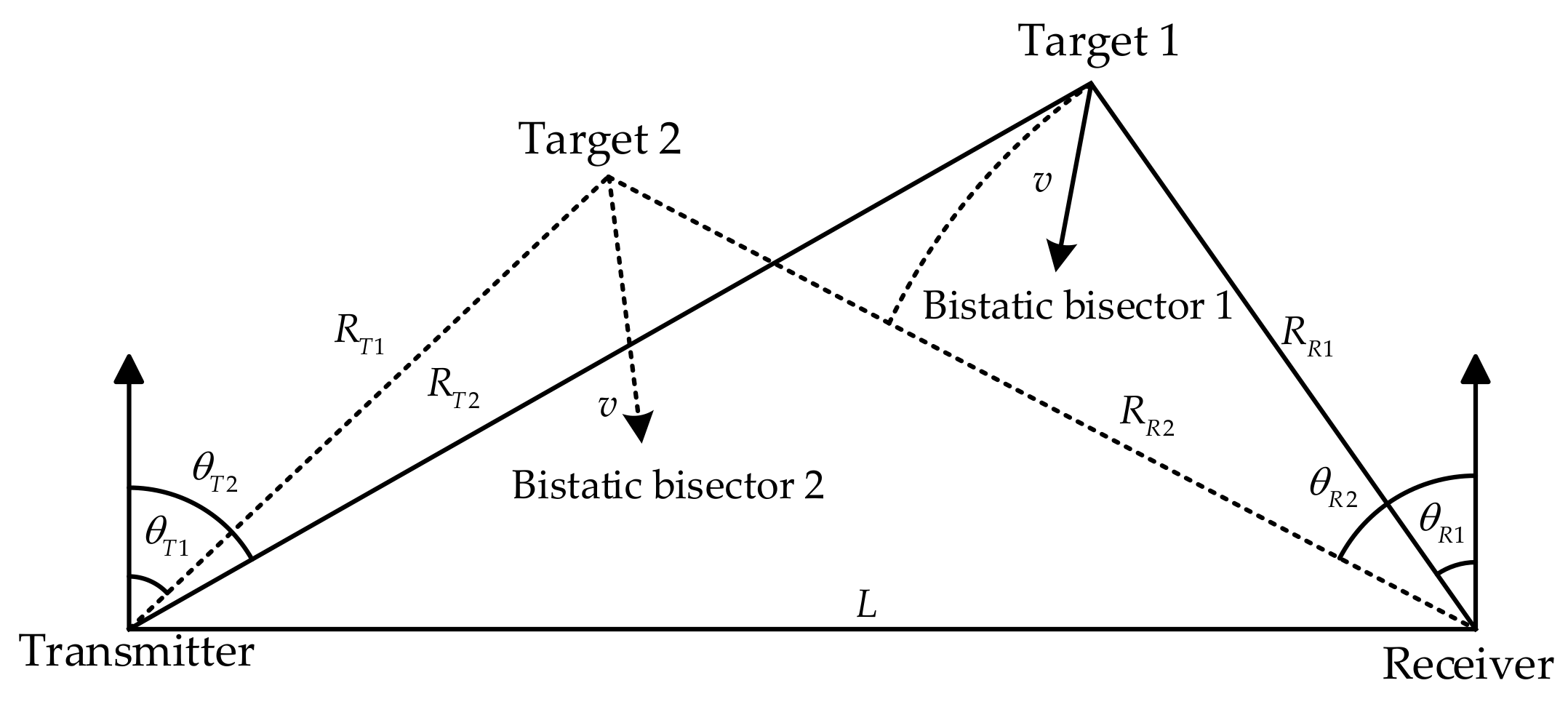
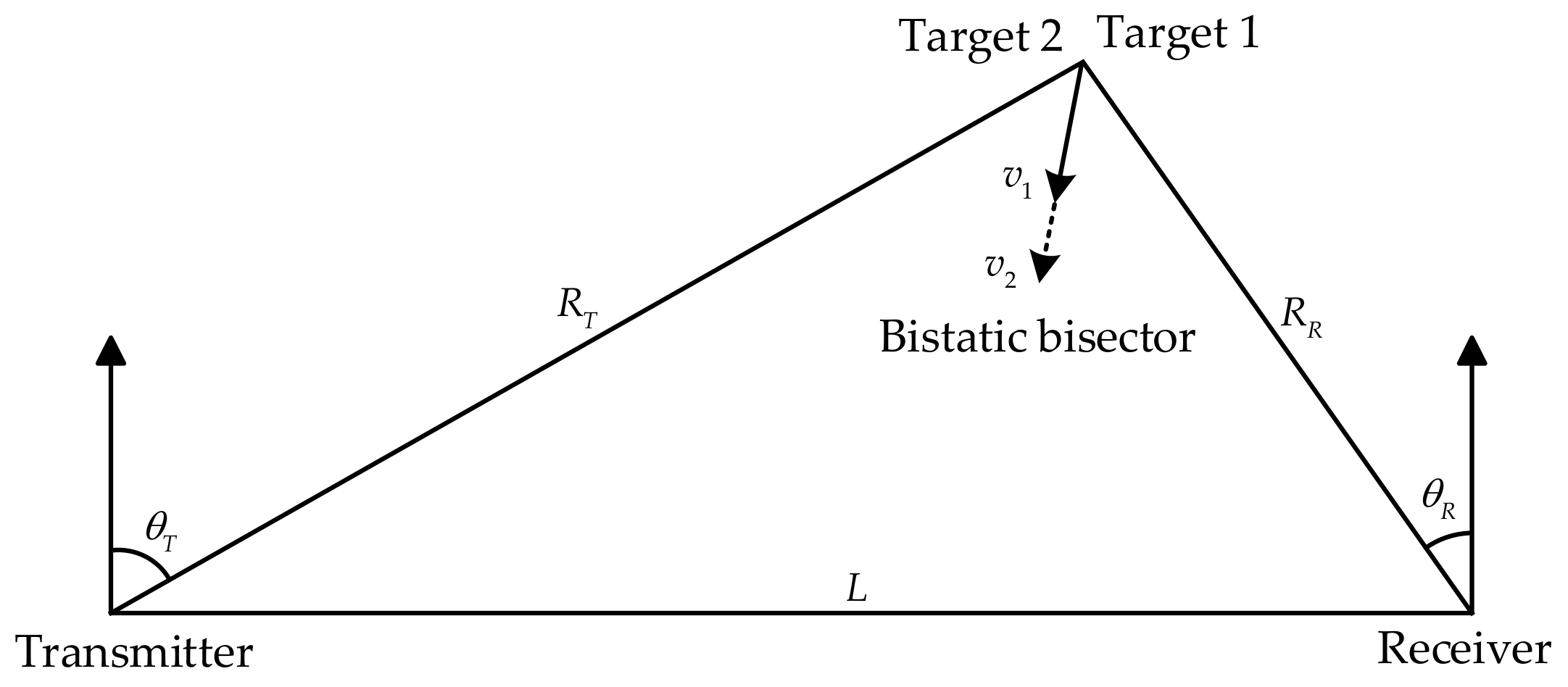
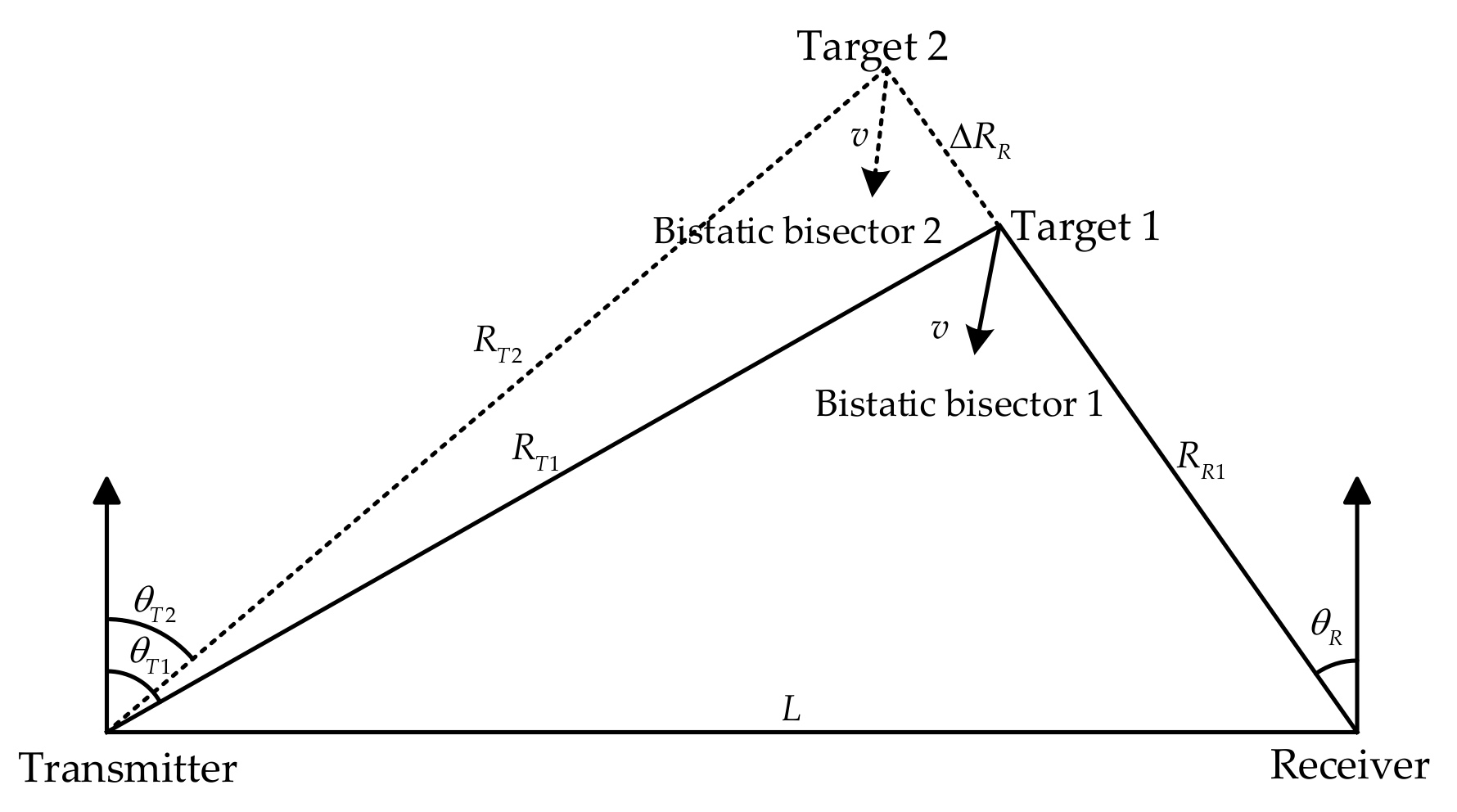
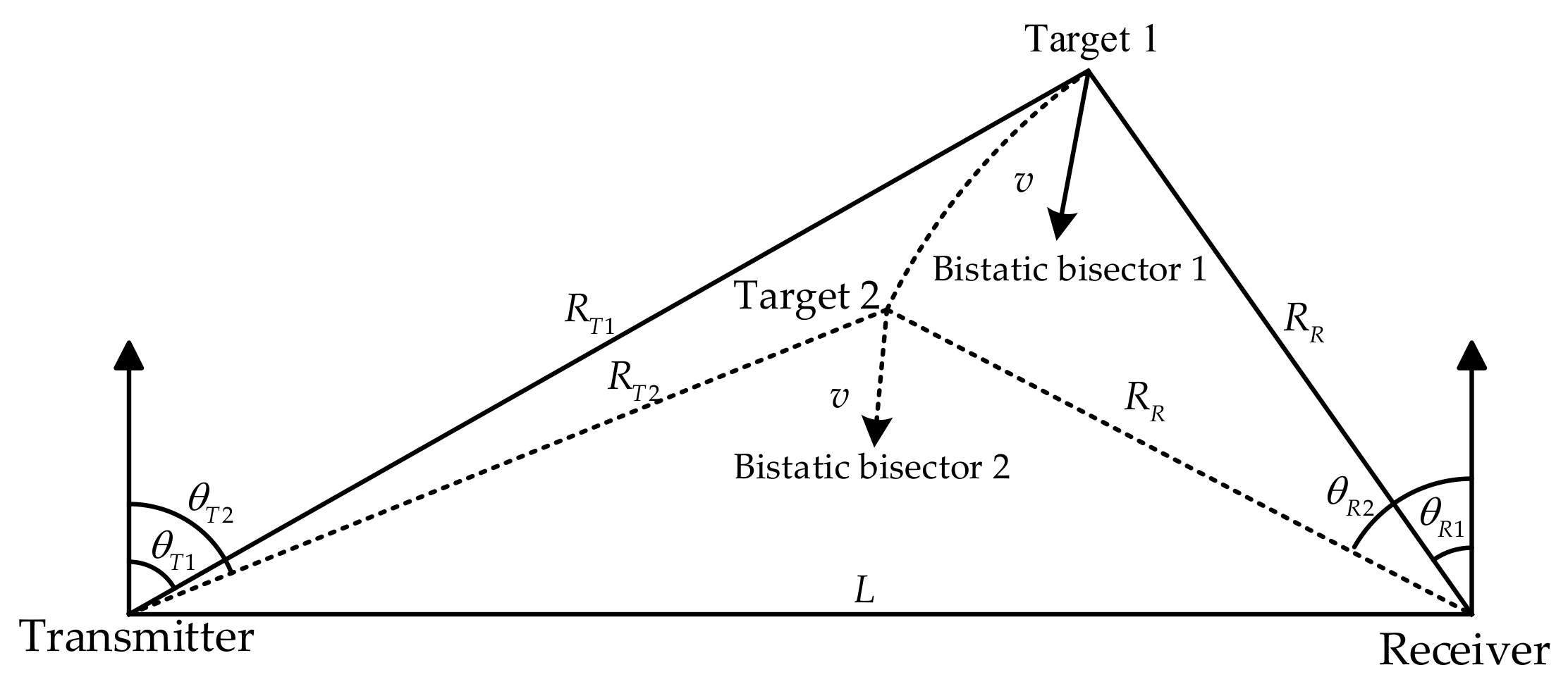
2.1. North-Referenced Coordinate System and Geometry of the Bistatic Radar

The geometric relationship in the bistatic radar is explained in this subsection. In the bistatic radar structure, the transmitter, receiver, and target form a plane triangle. By situating the bistatic radar geometric relationships within the North-referenced coordinate system [1], which is a 2D coordinate system, they become more understandable and transparent.

Figure 1 shows the bistatic radar within the coordinate system and its parameters. The upward direction in the picture corresponds to the north direction, which is the same as the map. Connecting the transmitter and the receiver is the bistatic baseline, whose length is $L$. The bistatic radar will reduce to the monostatic radar case when $L=0$. The look angle for the transmitter to target is called ${\theta }_T$, and ${\theta }_R$ for the receiver. They are limited to the range $\left[-\pi /2,3\pi /2\right]$ and are measured positive clockwise from the north of the coordinate system. The distance from the target to the transmitter and receiver is $R_T$ and $R_R$, respectively. The signal travels from the transmitter to the receiver via target reflection, with a total path length of $D$, and $D=R_T+R_R$. The bistatic angle $\beta$ is the angle in the bistatic triangle at the target, which is also at the apex, so that $\beta ={\theta }_T-{\theta }_R$. $\beta$ is in the interval $\left[0,\pi \right]$ when the target is to the north of the baseline and is negative and in the interval $\left[-\pi ,0\right]$ when the target is to the south of the baseline. The line bisects the bistatic angel $\beta$ is called the bistatic bisector. We are aware that the bistatic radar geometry can be fully defined using any three of the six parameters, $R_T$, $R_R$, ${\theta }_T$, ${\theta }_R$, $L$, $\beta$. When applied to the bistatic triangle, assume that $R_R$, ${\theta }_R$, and $L$ are known, and according to the law of cosines, $R_T$, ${\theta }_T$, $\beta$, and $D$ can be displayed as

$$R_T=\sqrt{{R_R}^2+L^2+2R_{R}L\sin {\theta }_R},$$

(1)

$${\theta }_T=\left\{\begin{array}{ll}{\sin }^{-1}{\displaystyle \frac{R_R\sin {\theta }_R+L}{\sqrt{{R_R}^2+L^2+2R_{R}L\sin {\theta }_R}}},& -\pi /2\le {\theta }_T\le \pi /2\hfill \\ \pi -{\sin }^{-1}{\displaystyle \frac{R_R\sin {\theta }_R+L}{\sqrt{{R_R}^2+L^2+2R_{R}L\sin {\theta }_R}}},& \pi /2\le {\theta }_T\le 3\pi /2\hfill \end{array}\right.,$$

(2)

$$\beta ={\theta }_T-{\theta }_R,$$

(3)

$$D=R_R+\sqrt{{R_R}^2+L^2+2R_{R}L\sin {\theta }_R}.$$

(4)

Similar results are obtained when $R_T$, ${\theta }_T$, and $L$ are known, and $R_R$, ${\theta }_R$, $\beta$, and $D$ can also be obtained using the cosine theorem.

$$R_R=\sqrt{{R_T}^2+L^2-2R_{T}L\sin {\theta }_T},$$

(5)

$${\theta }_R=\left\{\begin{array}{ll}{\sin }^{-1}{\displaystyle \frac{R_T\sin {\theta }_T+L}{\sqrt{{R_T}^2+L^2-2R_{T}L\sin {\theta }_T}}},& -\pi /2\le {\theta }_R\le \pi /2\hfill \\ \pi -{\sin }^{-1}{\displaystyle \frac{R_T\sin {\theta }_T+L}{\sqrt{{R_T}^2+L^2-2R_{T}L\sin {\theta }_T}}},& \pi /2\le {\theta }_R\le 3\pi /2\hfill \end{array}\right.,$$

(6)

$$\beta ={\theta }_T-{\theta }_R,$$

(7)

$$D=R_T+\sqrt{{R_T}^2+L^2-2R_{T}L\sin {\theta }_T}.$$

(8)

Figure 1. Bistatic radar geometry.

Figure 1. Bistatic radar geometry.

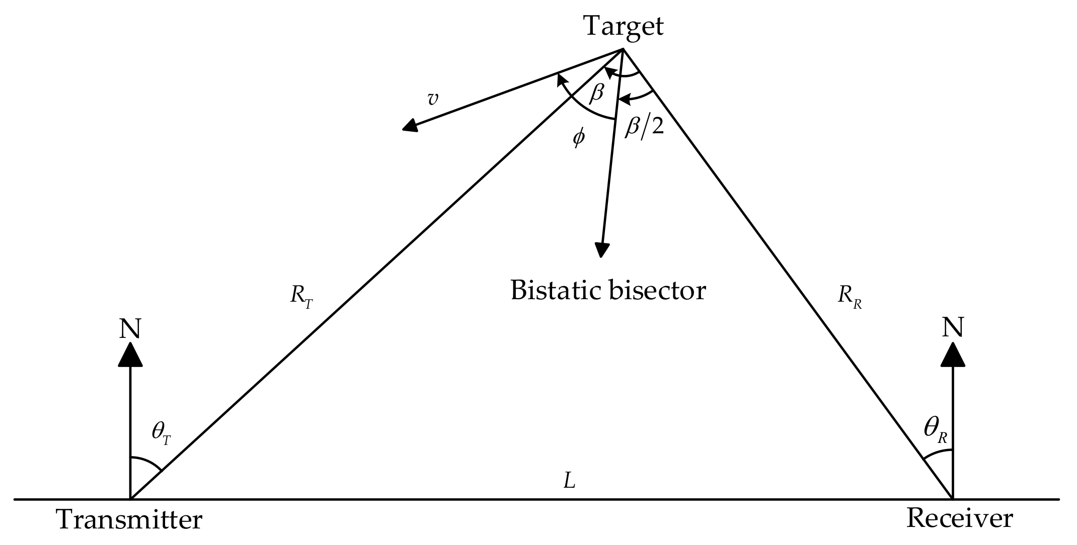
2.2. Effects of Bistatic Radar Geometry on the Time Delay and Doppler Shift

In this subsection, we figure out the manifestation of time delay and Doppler shift in the bistatic radar. Prior to the investigation, we clarify that all of the subsequent research items are slowly fluctuating point targets. A target can be considered as a slowly fluctuating point target under the following conditions:

• Slowly fluctuating target: If a target’s RCS remains relatively stable, exhibiting full pulse-to-pulse correlation within a scan period, and the amplitude distribution follows the Swerling III (chi square distribution) model (when the target is a primary scatterer), it can be considered as a slowly fluctuating target;
• Point target: Assume that there is a target in the propagation direction of an electromagnetic pulse which has scatterers distributed over the range interval $\left(R_1,R_2\right)$. Let $t_i$ represent the moment at which the pulse’s leading edge enters range $R_i$, where $i=1,2$. The moment the leading edge of the pulse emerges at the transmitting antenna is assumed to be the time origin. If $T$ denotes the duration of the transmitted pulse, the target can be treated as a point target as long as $t_2-t_1\ll T$.

Then, we assume a slowly fluctuating point target with the velocity $v$. The angle formed by velocity $v$ and bistatic bisector, determined from the bisector in a positive clockwise direction, is $\varphi$, which is shown in Figure 1. It is worth considering the time delay and Doppler shift of the target in the bistatic radar, which will become more complex than the monostatic radar due to the geometric factors caused by the separation of transmitter and receiver. Primarily, we must define the reference point because the radar’s transmitter and receiver are not in the same location. The relative position (time delay) and velocity (Doppler shift) of the target need to be determined with respect to this reference point, which can be the transmitter site, receiver site, or any other point in the plane. In view of this, we are interested in analyzing the corresponding variation in the receiver response with regard to the relative location, velocity, and angle, so the receiver site is the most suitable reference point for the investigation. In this case, $R_R$, ${\theta }_R$, and $L$ are used as the position parameters. Of course, similar conclusions can be drawn by selecting other reference points.

Based on the above, we conducted research on the time delay and Doppler shift issues of the bistatic radar, selecting the receiver site as the reference point. First, we consider the time delay. From (4), the total time delay $\tau \left(R_R,{\theta }_R,L\right)$ from the transmitter through the target to the receiver can obviously be given by

$$\tau \left(R_R,{\theta }_R,L\right)={\displaystyle \frac{R_R+\sqrt{{R_R}^2+L^2+2R_{R}L\sin {\theta }_R}}{c}},$$

(9)

where $c$ is the wave propagation speed. Evidently, (9) reduces to the monostatic radar case when $L=0$.

Next, we turn our attention to the Doppler shift. For simplicity’s sake, we suppose that the target is north of the baseline and that the transmitter and receiver are both stationary. By symmetry, the same result can be generated for the case in which the target is south of the baseline. It is clear that

$${\displaystyle \frac{d}{dt}}{R}_T=v\cos \left(\varphi -\beta /2\right),$$

(10)

$${\displaystyle \frac{d}{dt}}{R}_R=v\cos \left(\varphi +\beta /2\right),$$

(11)

$${\displaystyle \frac{d}{dt}}D=2v\cos \varphi \cos \left(\beta /2\right).$$

(12)

The factor $\cos \left(\beta /2\right)$ indicates that the resulting range rate is lower in the bistatic radar than in the monostatic case, and (12) reduces to the monostatic radar case when $\beta =0$. Further calculation leads to

$$\cos \left(\beta /2\right)=\sqrt{{\displaystyle \frac{1+\cos \beta }{2}}},$$

(13)

$$\cos \beta ={\displaystyle \frac{{R_T}^2+{R_R}^2-L^2}{2R_T{R}_R}}.$$

(14)

Substituting (4), (13), (14) into (12), we can obtain

$${\displaystyle \frac{d}{dt}}D=2v\cos \varphi \sqrt{{\displaystyle \frac{1}{2}}+{\displaystyle \frac{R_R+L\sin {\theta }_R}{2\sqrt{{R_R}^2+L^2+2R_{R}L\sin {\theta }_R}}}}.$$

(15)

After that, the Doppler shift $f_d$ along the bisector for a specific target velocity component becomes

$$f_d=2{\displaystyle \frac{f}{c}}v\cos \varphi \sqrt{{\displaystyle \frac{1}{2}}+{\displaystyle \frac{R_R+L\sin {\theta }_R}{2\sqrt{{R_R}^2+L^2+2R_{R}L\sin {\theta }_R}}}},$$

(16)

where $f$ is the carrier frequency. If the transmitter site is selected to be the reference point, we can obtain a similar conclusion

$$f_d=2{\displaystyle \frac{f}{c}}v\cos \varphi \sqrt{{\displaystyle \frac{1}{2}}+{\displaystyle \frac{R_T-L\sin {\theta }_T}{2\sqrt{{R_R}^2+L^2-2R_{T}L\sin {\theta }_T}}}}.$$

(17)

It is evident that (16) and (17) reduce to the monostatic radar case when $L=0$.

So far, the analysis has explained the geometry of the bistatic radar and demonstrated how time delay and Doppler shift occur in bistatic radars by taking into account the bistatic triangle and goal velocity when adding geometry components. In the next section, we consider bistatic FDA radar’s signal model and GAF.

3. Generalized Ambiguity Function of Bistatic FDA Radar

The GAF of the bistatic FDA radar is derived in this section. Firstly, we present the signal model of the bistatic FDA radar, and secondly, the bistatic FDA radar’s GAF is obtained on this basis.

3.1. Signal Model of Bistatic FDA Radar

In this subsection, we explore the signal model of bistatic FDA radar. The bistatic FDA radar transmitter is modeled as a uniform linear array (ULA) composed of $M$ identical radiating elements with a fixed interelement spacing $d_T$, as illustrated in Figure 2a. The radiated frequency of such FDA from the $(m+1)\mathrm{th}$ element is

$$f_m=f_0+\Delta f_m,m=0,1,\dots ,M-1,$$

(18)

where $f_0$ and $\Delta f$ represent carrier frequency and frequency offset, respectively. Then, the radio signal emitted from the $(m+1)\mathrm{th}$ element can be expressed as

$${\phi }_m\left(t\right)=w_{m}s\left(t\right)e^{j2\pi f_{m}t}.$$

(19)

Here, $w_m$ denotes the $(m+1)\mathrm{th}$ complex weight, and $s\left(t\right)$ represents the baseband waveform characterized by a duration $T_d$ and bandwidth $B_s$. Without loss of generality, $s\left(t\right)$ is assumed to have unitary energy, i.e., ${\displaystyle {\int }_0^{T_d}s\left(t\right)s^{*}\left(t\right)}dt=1$, where ${\left(\cdot \right)}^{*}$ denotes the complex conjugate. Let $s_m\left(t\right)=w_{m}s\left(t\right)$ denote the baseband signal for the $(m+1)\mathrm{th}$ element, (19) can be reformulated as

$${\phi }_m\left(t\right)=s_m\left(t\right)e^{j2\pi f_{m}t}.$$

(20)

The bistatic FDA radar receiver adopts an array structure analogous to the transmitter, comprising $N$ identical radiating elements with a fixed interelement spacing $d_R$, as depicted in Figure 2b.

Figure 2. Array structure: (a) Illustration of bistatic FDA radar transmitter. (b) Illustration of bistatic FDA radar receiver.

Figure 2. Array structure: (a) Illustration of bistatic FDA radar transmitter. (b) Illustration of bistatic FDA radar receiver.

Now, assume a slowly fluctuating point target with the velocity $v$ in the bistatic FDA radar space, which is assumed to satisfy the far-field condition for both the transmitter and receiver. Consequently, the transmission angle from the target to all transmitting elements is denoted as ${\theta }_T$, while the reception angle from the target to all receiving elements is denoted as ${\theta }_R$. Let $R_T$ and $R_R$ denote the distances from the target to the transmitter and receiver, respectively. From this perspective, the geometric configuration of the transmitter, receiver, and target is depicted in Figure 1. Given that the ambiguity function focuses on the received signal, the geometric relationships are therefore established with the receiver as the reference point. Hence, the time delay and Doppler shift are consistent with (9) and (16), respectively. Based on Equation (20), the expression for the echo signal received by the $(n+1)\mathrm{th}$ receiving element of the FDA transmitter is derived

$$\begin{array}{ll}{y}_n\left(t,\mathrm{\Theta }\right)& ={\displaystyle \sum _{m=0}^{M-1}{\phi }_m\left(t-{\tau }_{m,n}\left(\mathrm{\Theta }\right)\right)}\hfill \\ & \approx s\left(t-{\tau }_D\right){\displaystyle \sum _{m=0}^{M-1}{w}_m{e}^{j2\pi \left(f_0+\Delta f_m\right)\left[t-{\tau }_R+{\tau }_m\left({\theta }_T\right)+{\tau }_n\left({\theta }_R\right)\right]}}{e}^{j2\pi f_{d}t}\hfill \end{array},$$

(21)

$${\tau }_D={\displaystyle \frac{R_R+R_T}{c}},$$

(22)

$${\tau }_m\left({\theta }_T\right)=-{\displaystyle \frac{m{d}_T\sin {\theta }_T}{c}},$$

(23)

$${\tau }_n\left({\theta }_R\right)=-{\displaystyle \frac{n{d}_R\sin {\theta }_R}{c}}.$$

(24)

where $\mathrm{\Theta }\triangleq \left\{R_T,R_R,{\theta }_T,{\theta }_R,f_d\right\}$ is the target parameter set of interest.

3.2. Generalized Ambiguity Function of Bistatic FDA Radar

In conventional radar systems, the ambiguity function is mathematically defined as the cross-correlation between the radar waveform $s\left(t\right)$ and its time-delayed $\Delta \tau$ and frequency-shifted $\Delta f_d$ version, that is

$${\chi }_{ss}\left(\Delta \tau ,\Delta f_d\right)\triangleq {\displaystyle {\int }_{-\infty }^{\infty }s\left(t\right)s^{*}\left(t-\Delta \tau \right)e^{-j2\pi \Delta f_{d}t}dt}.$$

(25)

While the conventional ambiguity function is restricted to evaluating the range–Doppler resolution of traditional SISO radars. The GAF for bistatic FDA radar should encompass target range, angle, and velocity parameters, which can be defined as

$${\chi }_{\mathrm{FDA}}\left({\mathrm{\Theta }}_1,{\mathrm{\Theta }}_2\right)={\displaystyle \sum _{n=0}^{N-1}{\displaystyle {\int }_{-\infty }^{\infty }{y}_n\left(t,{\mathrm{\Theta }}_1\right)y_n^{*}\left(t,{\mathrm{\Theta }}_2\right)}}dt,$$

(26)

where ${\mathrm{\Theta }}_1\triangleq \left\{R_{T1},R_{R1},{\theta }_{T1},{\theta }_{R1},f_{d1}\right\}$, ${\mathrm{\Theta }}_2\triangleq \left\{R_{T2},R_{R2},{\theta }_{T2},{\theta }_{R2},f_{d2}\right\}$ is the parameter of two targets, respectively. Substituting Equation (21) into Equation (26) yields

$$\begin{array}{ll}{\chi }_{\mathrm{FDA}}\left({\mathrm{\Theta }}_1,{\mathrm{\Theta }}_2\right)& =e^{-j2\pi f_0\left({\tau }_{D1}-{\tau }_{D2}\right)}{\displaystyle \sum _{n=0}^{N-1}{e}^{j2\pi f_0\left[{\tau }_n\left({\theta }_{R1}\right)-{\tau }_n\left({\theta }_{R2}\right)\right]}}\hfill \\ & {\displaystyle {\int }_{-\infty }^{\infty }s\left(t-{\tau }_{D1}\right)}{s}^{*}\left(t-{\tau }_{D2}\right)e^{j2\pi \left(f_{d1}-f_{d2}\right)t}\hfill \\ & {\displaystyle \sum _{m=0}^{M-1}{\displaystyle \sum _{m^{\prime }=0}^{M-1}{w}_m{w}_{m^{\prime }}^{*}{e}^{j2\pi f_0\left[{\tau }_m\left({\theta }_{T1}\right)-{\tau }_{n^{\prime }}\left({\theta }_{T2}\right)\right]}}}{e}^{-j2\pi \left[\Delta f_m{\tau }_{R1}-\Delta f_{m^{\prime }}{\tau }_{R2}\right]}{e}^{j2\pi \left(\Delta f_m-\Delta f_{m^{\prime }}\right)t}dt\hfill \end{array},$$

(27)

where ${\tau }_D$, $f_d$ have been given previously. Set $\Delta \tau \triangleq {\tau }_{D1}-{\tau }_{D2}$, $\Delta f_d\triangleq f_{d2}-f_{d1}$, $\tau =t-{\tau }_{D1}$, and drop the irrelevant terms to obtain

$$\begin{array}{ll}{\chi }_{\mathrm{FDA}}& ={\displaystyle \sum _{n=0}^{N-1}{e}^{j2\pi f_0\left[{\tau }_n\left({\theta }_{R1}\right)-{\tau }_n\left({\theta }_{R2}\right)\right]}}\hfill \\ & {\displaystyle \hspace{1em}{\int }_{-\infty }^{\infty }s\left(\tau \right)s^{*}\left(t-\Delta \tau \right)e^{j2\pi \Delta f_d\left(\tau +{\tau }_{D1}\right)}}\\ & \hspace{1em}{\displaystyle \sum _{m=0}^{M-1}{\displaystyle \sum _{m^{\prime }=0}^{M-1}{w}_m{w}_{m^{\prime }}^{*}{e}^{j2\pi f_0\left[{\tau }_m\left({\theta }_{T1}\right)-{\tau }_{n^{\prime }}\left({\theta }_{T2}\right)\right]}{e}^{j2\pi \Delta f_{m^{\prime }}\left({\tau }_{D2}-t\right)}{e}^{j2\pi \Delta f_m\left(t-{\tau }_{D1}\right)}d\tau }}\\ & ={\displaystyle \sum _{n=0}^{N-1}{e}^{j2\pi f_0\left[{\tau }_n\left({\theta }_{R1}\right)-{\tau }_n\left({\theta }_{R2}\right)\right]}}\hfill \\ & \hspace{1em}{\displaystyle \sum _{m=0}^{M-1}{\displaystyle \sum _{m^{\prime }=0}^{M-1}{w}_m{w}_{m^{\prime }}^{*}{e}^{j2\pi f_0\left[{\tau }_m\left({\theta }_{T1}\right)-{\tau }_{n^{\prime }}\left({\theta }_{T2}\right)\right]}}}{e}^{j2\pi \Delta f_{m^{\prime }}\Delta \tau }\hfill \\ & \hspace{1em}{\displaystyle {\int }_{-\infty }^{\infty }s\left(\tau \right)s^{*}\left(\tau -\Delta \tau \right)e^{j2\pi \left(\Delta f_d+\Delta f_m-\Delta f_{m^{\prime }}\right)\tau }d\tau }\hfill \end{array}$$

(28)

Expressed in matrix and vector form:

$${\chi }_{\mathrm{FDA}}\left({\mathrm{\Theta }}_1,{\mathrm{\Theta }}_2\right)=a_r^H\left({\theta }_{R1}\right)a_r\left({\theta }_{R2}\right){\left[a_t\left({\theta }_{T2}\right)\odot g^{*}\left(\Delta \tau \right)\right]}^H\chi a_t\left({\theta }_{T1}\right),$$

(29)

$$a_R\left({\theta }_R\right)={\left[1,e^{j2\pi f_{0}d\sin {\theta }_R/c},\cdots ,e^{j2\pi f_0\left(N-1\right)d\sin {\theta }_R/c}\right]}^T,$$

(30)

$$a_T\left({\theta }_T\right)={\left[1,e^{j2\pi f_{0}d\sin {\theta }_T/c},\cdots ,e^{j2\pi f_0\left(M-1\right)d\sin {\theta }_R/c}\right]}^T,$$

(31)

$$g\left(\Delta \tau \right)={\left[1,e^{j2\pi \Delta f_1\Delta \tau },\cdots ,e^{j2\pi \Delta f_{M-1}\Delta \tau }\right]}^T,$$

(32)

$$\chi =\left[\begin{array}{ccc}{\chi }_s\left(\Delta \tau ,\Delta f_d\right)& \dots & {\chi }_s\left(\Delta \tau ,\Delta f_d-\Delta f_{M-1}\right)\\ ⋮& \ddots & ⋮\\ {\chi }_s\left(\Delta \tau ,\Delta f_d+\Delta f_{M-1}\right)& \dots & {\chi }_s\left(\Delta \tau ,\Delta f_d+\Delta f_{M-1}-\Delta f_{M-1}\right)\end{array}\right],$$

(33)

where $\chi \in {ℂ}^{M\times M}$ is the conventional ambiguity function of the transmitted baseband signal. When $R_{T1}=R_{T2}$, $R_{R1}=R_{R2}$, ${\theta }_{T1}={\theta }_{T2}$, ${\theta }_{R1}={\theta }_{R2}$, and $L=0$, Equation (29) reduces to the conventional ambiguity function of monostatic FDA radar.

Analysis of the GAF model for bistatic FDA radar reveals that, beyond the common waveform parameters shared with monostatic FDA systems (baseband waveform and frequency offsets), the bistatic FDA radar’s GAF inherently incorporates geometric dependencies through time delay and Doppler shift. This geometric information includes the baseline length of the bistatic radar, the reception distance, and angle (with the receiver site as the reference point). This establishes a dual influence mechanism where both FDA transmitted signal properties and bistatic geometry jointly govern GAF performance, constituting a defining feature of bistatic radar system. Subsequent numerical simulations will systematically investigate what effect they have on GAF.

3.3. Computational Complexity Analysis and Practical Application Limitations of Bistatic FDA Radar’s GAF

Once the bistatic FDA radar configuration is determined, parameters including the number of transmit/receive array elements, baseband waveform of the FDA array’s transmitted signal, and bistatic baseline length become fixed. Under these circumstances, we analyze the Big O notation computational complexity when applying Equations (29)–(33) to compute the GAF of bistatic FDA radar in this subsection:

• $a_r^H\left({\theta }_{R1}\right)a_r\left({\theta }_{R2}\right)$ represents a Hermitian inner product of two N-dimensional vectors. Each element-wise multiplication and summation contributes $\mathcal{O}\left(N\right)$ complexity.
• The Hadamard product $a_t\left({\theta }_{T2}\right)\odot g^{*}\left(\Delta \tau \right)$ involves element-wise multiplication of two M-dimensional vectors, resulting in $\mathcal{O}\left(M\right)$ complexity.
• ${\left[a_t\left({\theta }_{T2}\right)\odot g^{*}\left(\Delta \tau \right)\right]}^H\chi a_t\left({\theta }_{T1}\right)$, with $\chi$ is an M × M matrix, the operation combines a 1 × M vector, an M × M matrix, and an M × 1 vector. Matrix–vector multiplication for an M × M matrix and M–vector dominates with $\mathcal{O}\left(M^2\right)$ complexity.

Summing these contributions, the total complexity is $\mathcal{O}(M^2+M+N)$. By the principle of dominant-term analysis in computational complexity (where higher-order terms govern asymptotic behavior), $M^2$ grows significantly faster than $M$. Thus, the complexity simplifies to $\mathcal{O}(M^2+N)$, as the $M^2$ term overshadows the $M$ term, leaving $\mathcal{O}(M^2+N)$ as the complexity expression. This demonstrates that the computational complexity of the bistatic FDA radar GAF is determined by the quantities of transmitting (M) and receiving (N) array elements.

In practical implementations, radar systems often employ substantial quantities of transmit/receive array elements and adopt complex geometries such as conformal or planar arrays rather than conventional ULA. Thus, the computational complexity of calculating the GAF for bistatic radar may remain relatively high in practical applications, which is one of the potential limitations of this algorithm.

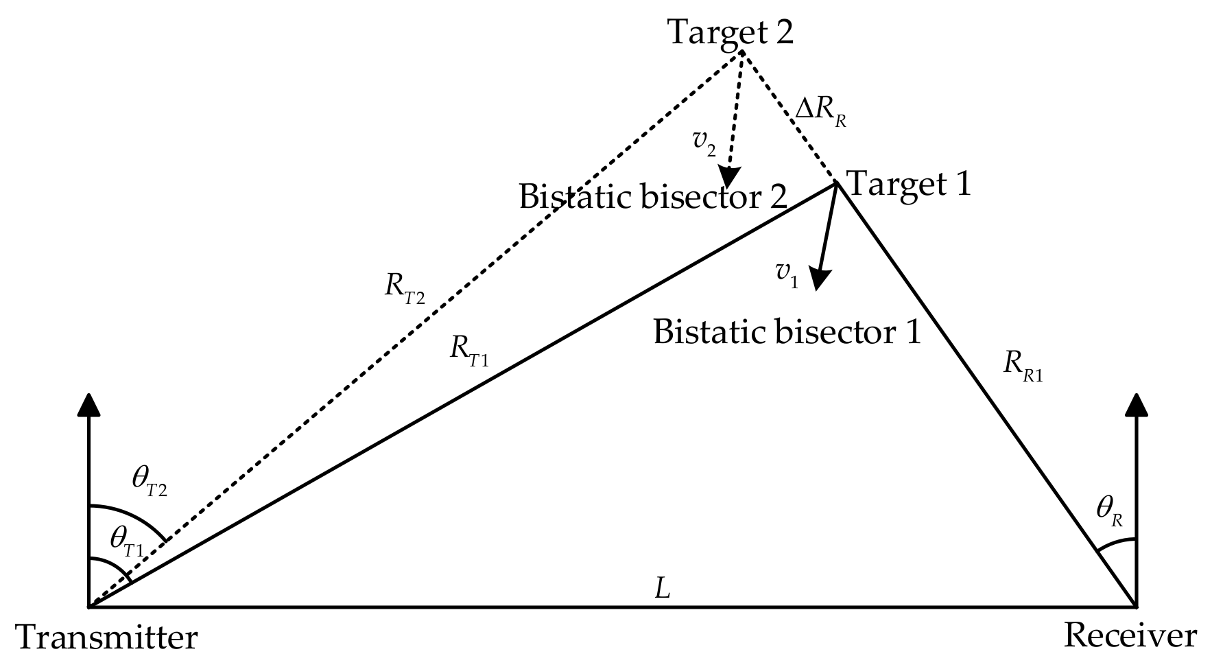
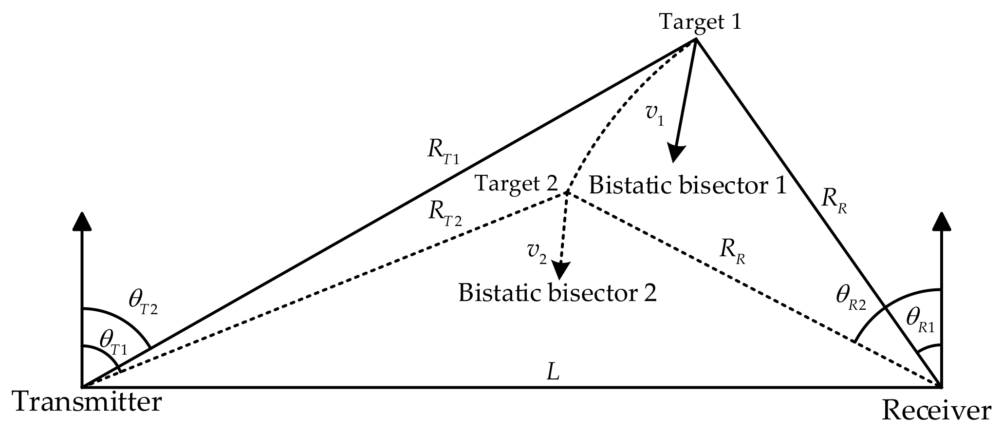
4. Numerical Simulations and Analysis

This section employs numerical simulations to investigate the GAF of bistatic FDA radar. Firstly, Subsection 4.1 and Subsection 4.2 analyze the effects of transmitted signal properties and bistatic geometries on the bistatic FDA radar GAF. Secondly, Subsection 4.3 compares the GAFs of bistatic and monostatic FDA radars (monostatic as baseline algorithm), revealing the key differences between them.

As previously established, the GAF analysis focuses on targets’ range, velocity, and angle resolution specifically at the receiver of the bistatic radar system. Consequently, the receiver site is selected as the reference point in this study, with parameters $R_R$, ${\theta }_R$ and $L$ constituting the primary variables under investigation. Without loss of generality, the target velocity is assumed to align with the bistatic bisector ($\varphi =0,\cos \varphi =1$). This strategic simplification streamlines the analytical process while preserving the fundamental properties of the bistatic FDA radar’s GAF.

We implement a uniform linear FDA array composed of $M$ identical radiating elements with inter-element spacing $d_T=\lambda /2$ at the bistatic radar transmitter (similarly, the receiver is modeled as a ULA with $N$ identical radiating elements and fixed interelement spacing $d_R=\lambda /2$), which is shown in Figure 2, for this study.

In addition, it is imperative to formalize the simulation framework in this study. First, we define the parameters:

• The bistatic baseline length $L$;
• Reception distance $R_{R1}$, reception angle, ${\theta }_{R1}$ and velocity $v_1$ of Target 1, which is regarded as the reference target, and the direction of velocity parameter $v_1$ is along the bistatic bisector;
• Parameters $\left(R_{R2},{\theta }_{R2},v_2\right)$ of Target 2, with the differential parameters relative to Target 1 are defined as $\Delta R_R=R_{R2}-R_{R1}$, $\Delta {\theta }_R={\theta }_{R2}-{\theta }_{R1}$, $\Delta v=v_2-v_1$.

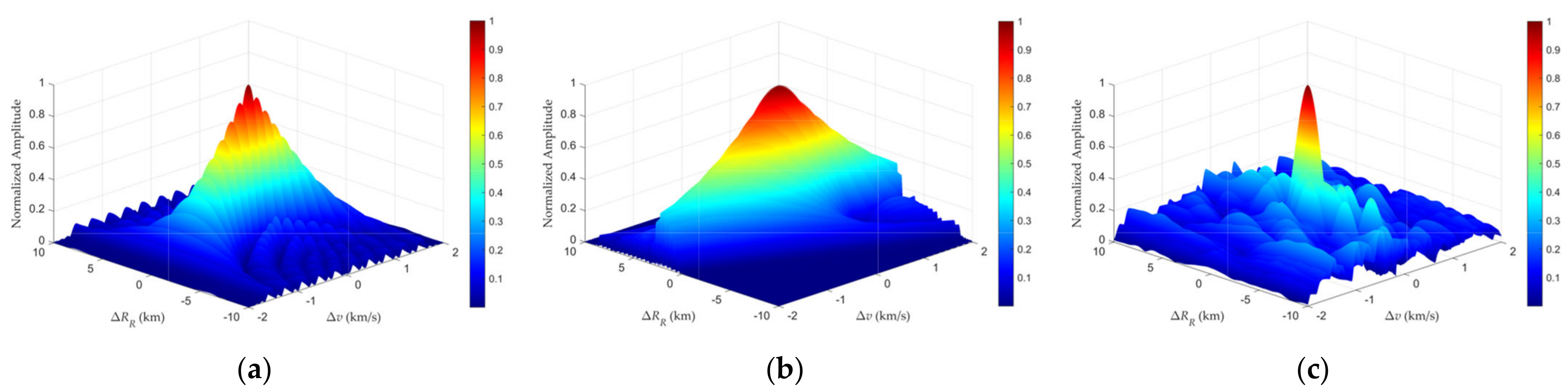
4.1. Influence of Transmitted Signal

We first investigate the influence of FDA transmitted signal parameters on the GAF of bistatic FDA radar through a systematic comparative framework. Two representative baseband waveforms were designed for analysis:

• Single-tone waveform $s_{\mathrm{ST}}\left(t\right)=1/\sqrt{T_d}\mathrm{rect}\left(t/T_d\right)$;
• Linear-frequency-modulated (LFM) waveform $s_{\mathrm{LFM}}=1/\sqrt{T_d}\mathrm{rect}\left(t/T_d\right)e^{j\pi \mu t^2}$,

where $\mathrm{rect}\left(\cdot \right)$ and $\mu =B_s/T_d$ represent the rectangular window function and chirp rate, respectively. The corresponding ambiguity functions can be expressed as

$${\chi }_{\mathrm{ST}}\left(\Delta \tau ,\Delta f_d\right)=\left(1-{\displaystyle \frac{\left|\Delta \tau \right|}{T_d}}\right){\displaystyle \frac{\sin \left[\pi \Delta f_d\left(T_d-\left|\Delta \tau \right|\right)\right]}{\pi \Delta f_d\left(T_d-\left|\Delta \tau \right|\right)}},\left|\Delta \tau \right|\le T_d,$$

(34)

$${\chi }_{\mathrm{LFM}}=\left(1-{\displaystyle \frac{\left|\Delta \tau \right|}{T_d}}\right){\displaystyle \frac{\sin \left[\pi T_d\left(\mu \Delta \tau -\Delta f_d\right)\left(1-\frac{\left|\Delta \tau \right|}{T_d}\right)\right]}{\pi T_d\left(\mu \Delta \tau -\Delta f_d\right)\left(1-\frac{\left|\Delta \tau \right|}{T_d}\right)}}.$$

(35)

For frequency offsets, two allocation schemes were implemented across FDA elements:

• Linear frequency offset $\Delta f_m=m\Delta f,m=0,1,\cdots ,M-1$;
• Random frequency offset $\Delta f_m=\delta \Delta f,\delta \sim \mathrm{N}\left(0,1\right)$.

Table 1. Values of the simulation parameters.

Parameter	$\mathit{M}$	$\mathit{N}$	${\mathit{f}}_{\mathbf{0}}$ (GHz)	$\mathbf{\Delta }\mathit{f}$ (kHz)	$\mathit{\mu }$ (MHz/s)
Value	12	10	10	10	500
Parameter	$T_d$(ms)	$v_1$(m/s)	$L$	$R_{R1}$	${\theta }_{R1}$(deg.)
Value	0.2	500	500	300	−30

summarizes the critical simulation parameters.

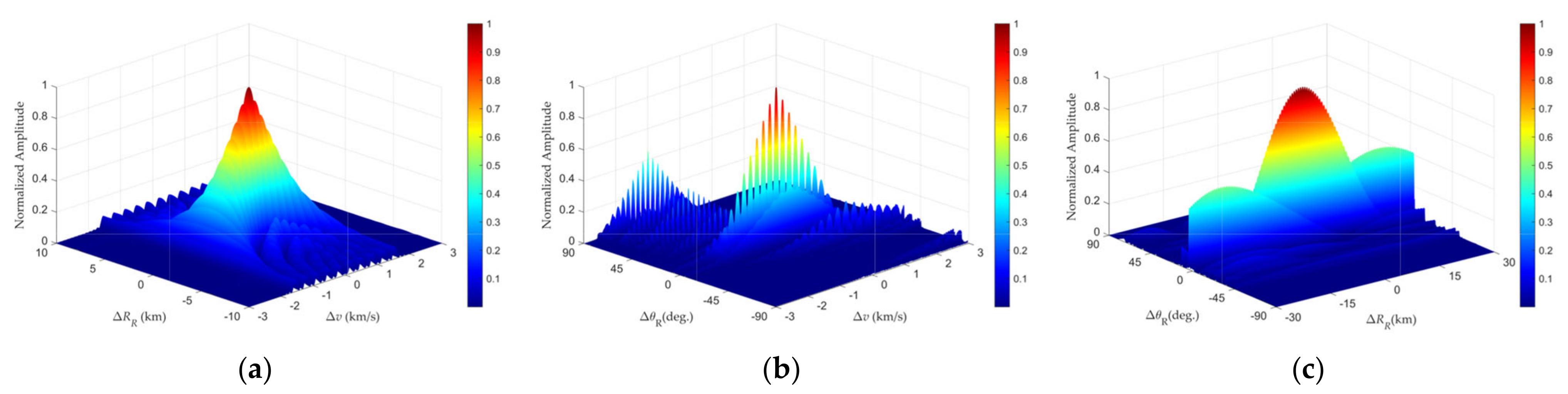
4.1.1. Range–Velocity GAF

Under this condition, letting Targets 1 and 2 share the same reception angle ${\theta }_{R2}={\theta }_{R1}={\theta }_R$, the reception distance difference between them is defined as $\Delta R_R=R_{R2}-R_{R1}$, while their velocity difference is given by $\Delta v=v_2-v_1$, which is shown in Figure 3. The spatial separation and velocity disparity between the two targets induce differential time delays ($\Delta \tau$) in echo signals and discernible Doppler shifts ($\Delta f_d$) in the received waveforms. $\Delta \tau$, $f_{d1}$, $f_{d2}$ and the range–velocity GAF of the bistatic FDA radar can consequently be expressed as

$$\Delta \tau ={\displaystyle \frac{\left(R_{R2}+R_{T2}\right)-\left(R_{R1}+R_{T1}\right)}{c}},$$

(36)

$$f_{d1}=2{\displaystyle \frac{f}{c}}{v}_1\sqrt{{\displaystyle \frac{1}{2}}+{\displaystyle \frac{R_{R1}+L\sin {\theta }_R}{2\sqrt{R_{R1}^2+L^2+2R_{R1}L\sin {\theta }_R}}}},$$

(37)

$$f_{d2}=2{\displaystyle \frac{f}{c}}{v}_2\sqrt{{\displaystyle \frac{1}{2}}+{\displaystyle \frac{R_{R2}+L\sin {\theta }_R}{2\sqrt{R_{R2}^2+L^2+2R_{R2}L\sin {\theta }_R}}}},$$

(38)

$${\chi }_{\Delta R_R-\Delta v}\left({\mathrm{\Theta }}_1,{\mathrm{\Theta }}_2\right)=a_r^H\left({\theta }_R\right)a_r\left({\theta }_R\right){\left[a_t\left({\theta }_{T1}\right)\odot g^{*}\left(\Delta \tau \right)\right]}^H\chi a_t\left({\theta }_{T2}\right),$$

(39)

where $a_r\left(\theta \right)$, $a_t\left(\theta \right)$, $\chi$ have been given previously.

As evidenced by Figure 4, both baseband waveform selection and frequency offset schemes modulate the velocity–range GAF morphology. Under linear uniform frequency offset conditions, both single-tone and LFM baseband waveforms exhibit pronounced velocity ambiguity artifacts and periodic spikes in the velocity dimension. This phenomenon will have a more evident and intuitive presentation in subsequent velocity GAF analyses, which is similar to that observed in monostatic FDA radar. Therefore, we can consider that ambiguity and periodic spikes are not related to the bistatic geometric configurations but are caused by the frequency offset in the transmitted signal of the FDA radar. Notably, the LFM waveform additionally demonstrates discernible side lobe broadening in the range dimension. Strikingly, employing random frequency offsets effectively mitigates these artifacts, eliciting a distinctive spike-shaped ambiguity function with suppressed side lobe.

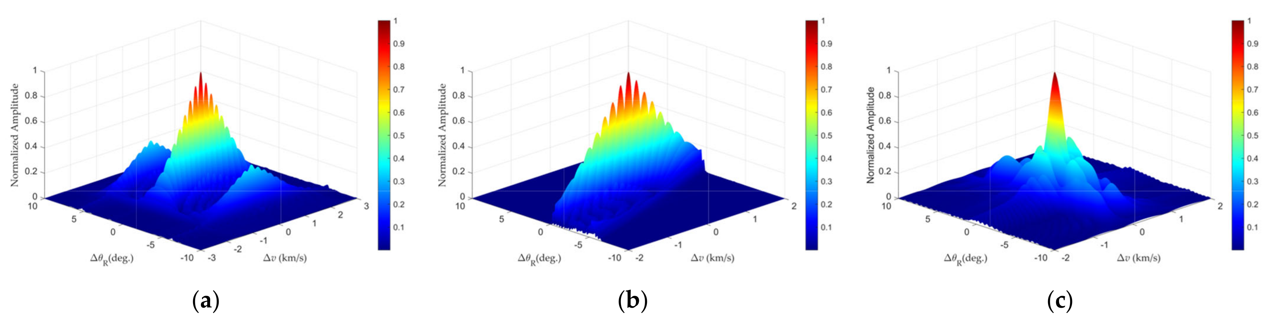
4.1.2. Angle–Velocity GAF

In this subsubsection, both Targets 1 and 2 are assigned identical reception distance $R_{R2}=R_{R1}=R_R$, while exhibiting a velocity difference of $\Delta v=v_2-v_1$ and a reception angle difference of $\Delta {\theta }_R={\theta }_{R2}-{\theta }_{R1}$, as is shown in Figure 5. The structural changes in the bistatic triangle also bring $\Delta \tau$ and $\Delta f_d$. $\Delta \tau$, $f_{d1}$, $f_{d2}$ and the angle–velocity GAF of the bistatic FDA radar can consequently be expressed as

$$\Delta \tau ={\displaystyle \frac{\left(R_R+R_{T2}\right)-\left(R_R+R_{T1}\right)}{c}},$$

(40)

$$f_{d1}=2{\displaystyle \frac{f}{c}}{v}_1\sqrt{{\displaystyle \frac{1}{2}}+{\displaystyle \frac{R_R+L\sin {\theta }_{R1}}{2\sqrt{R_R^2+L^2+2R_{R}L\sin {\theta }_{R1}}}}},$$

(41)

$$f_{d2}=2{\displaystyle \frac{f}{c}}{v}_2\sqrt{{\displaystyle \frac{1}{2}}+{\displaystyle \frac{R_R+L\sin {\theta }_{R2}}{2\sqrt{R_R^2+L^2+2R_{R}L\sin {\theta }_{R2}}}}},$$

(42)

$${\chi }_{\Delta {\theta }_R-\Delta v}\left({\mathrm{\Theta }}_1,{\mathrm{\Theta }}_2\right)=a_r^H\left({\theta }_{R2}\right)a_r\left({\theta }_{R1}\right){\left[a_t\left({\theta }_{T1}\right)\odot g^{*}\left(\Delta \tau \right)\right]}^H\chi a_t\left({\theta }_{T2}\right).$$

(43)

The angle–velocity GAF exhibits markedly distinct characteristics under different baseband waveform designs and frequency offset schemes, as demonstrated in Figure 6. The periodic peak characteristics of the velocity dimension under single-tone and LFM baseband waveforms with linear frequency offset persist, and the single-tone baseband is more pronounced in Figure 6. LFM waveforms with linear frequency offset achieve complete side lobe suppression in the angular domain at the expense of moderate main lobe broadening. Random frequency offset scheme generates near-ideal spike-type ambiguity functions, primarily eliminating velocity ambiguity.

4.1.3. Angle–Range GAF

Here, we consider Targets 1 and 2 to have equal velocity $v_1=v_2=v$, accompanied by a reception distance difference $\Delta R_R=R_{R2}-R_{R1}$ and a reception angle difference of $\Delta {\theta }_R={\theta }_{R2}-{\theta }_{R1}$ in reception, which is shown in Figure 7. $\Delta \tau$, $f_{d1}$, $f_{d2}$ and the angle–range GAF of the bistatic FDA radar can be expressed as

$$\Delta \tau ={\displaystyle \frac{\left(R_{R2}+R_{T2}\right)-\left(R_{R1}+R_{T1}\right)}{c}},$$

(44)

$$f_{d1}=2{\displaystyle \frac{f}{c}}v\sqrt{{\displaystyle \frac{1}{2}}+{\displaystyle \frac{R_{R1}+L\sin {\theta }_{R1}}{2\sqrt{R_{R1}^2+L^2+2R_{R1}L\sin {\theta }_{R1}}}}},$$

(45)

$$f_{d2}=2{\displaystyle \frac{f}{c}}v\sqrt{{\displaystyle \frac{1}{2}}+{\displaystyle \frac{R_{R2}+L\sin {\theta }_{R2}}{2\sqrt{R_{R2}^2+L^2+2R_{R2}L\sin {\theta }_{R2}}}}},$$

(46)

$${\chi }_{\Delta {\theta }_R-\Delta R_R}\left({\mathrm{\Theta }}_1,{\mathrm{\Theta }}_2\right)=a_r^H\left({\theta }_{R2}\right)a_r\left({\theta }_{R1}\right){\left[a_t\left({\theta }_{T1}\right)\odot g^{*}\left(\Delta \tau \right)\right]}^H\chi a_t\left({\theta }_{T2}\right),$$

(47)

Figure 8 illustrates the 3D and 2D representations of range–angle GAF under various baseband waveform and frequency offsets configurations. These factors affect the GAF’s shape, yet both the main or side lobes exhibit some trailing due to the range–angle coupling of FDA radar. For the single-tone waveform with linear frequency offset, this trailing is evident in both the main and side lobes. In the LFM baseband with linear frequency offset, the GAF suppresses side lobes, creating a main lobe with significant trailing. Random frequency offset reduces trailing and suppresses side lobes more than single-tone waveform with linear frequency offset does, but it does not produce the sharp main lobe seen in range–velocity and angle–velocity GAFs.

4.2. Influence of Bistatic Geometric Configurations

This part systematically investigates the impact of bistatic radar geometric configurations on the GAF. Prior to initiating numerical simulations, the experimental parameters are systematically established.

Table 2. Values of the invariant parameters.

Parameter	$\mathit{M}$	$\mathit{N}$	${\mathit{f}}_0$ (GHz)	$\mathbf{∆}\mathit{f}$ (kHz)	${\mathit{T}}_{\mathit{d}}$ (ms)	${\mathit{v}}_1$ (m/s)
Value	12	10	10	10	0.2	500

enumerates the invariant parameters used throughout the experiment.

Table 3. Values of the variable parameters.

	$\mathit{L}$ (km)	${\mathit{R}}_{\mathit{R}1}$ (km)	${\mathit{\theta }}_{\mathit{R}1}$ (deg.)
Case 1	100	300	−30
Case 2	500	300	−30
Case 3	1500	300	−30
Case 4	500	80	−30
Case 5	500	300	−30
Case 6	500	1300	−30
Case 7	500	300	−30
Case 8	500	300	0
Case 9	500	300	60

details the variable parameters modified to generate distinct bistatic geometric configurations, which systematically vary three bistatic parameters:

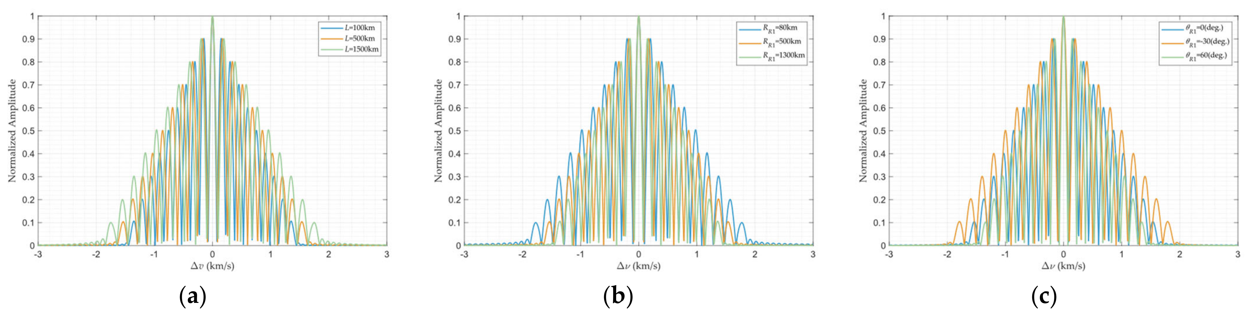
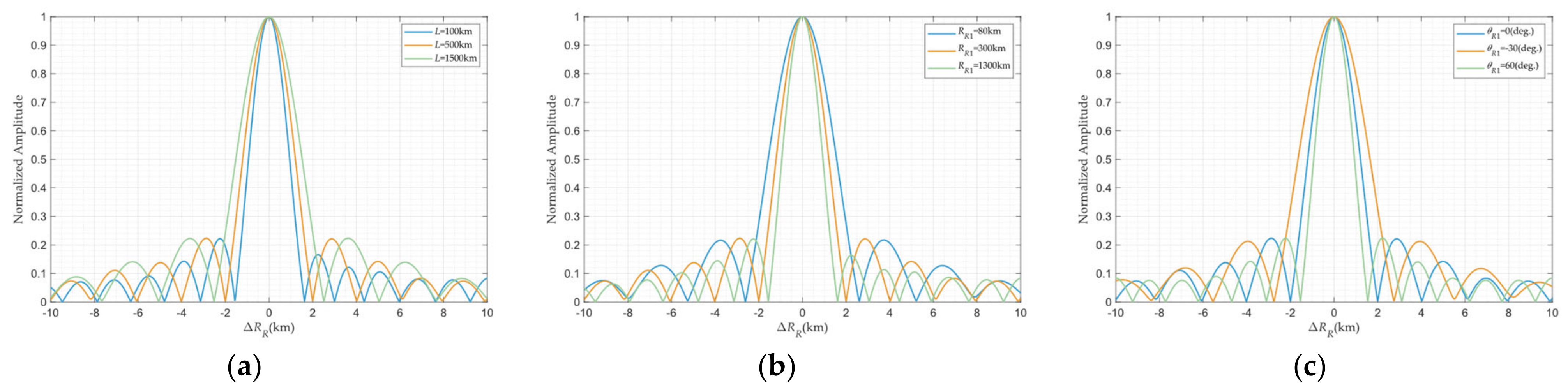
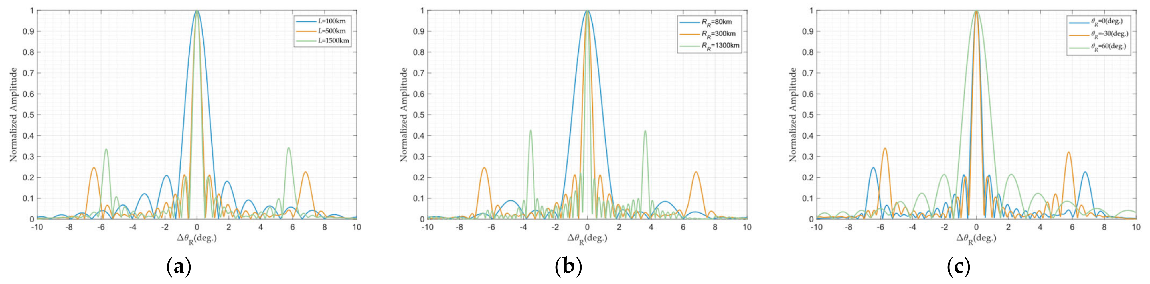
• Cases 1–3 modify baseline length $L$;
• Cases 4–6 adjust target–receiver range $R_{R1}$;
• Cases 7–9 alter reception angle ${\theta }_{R1}$.

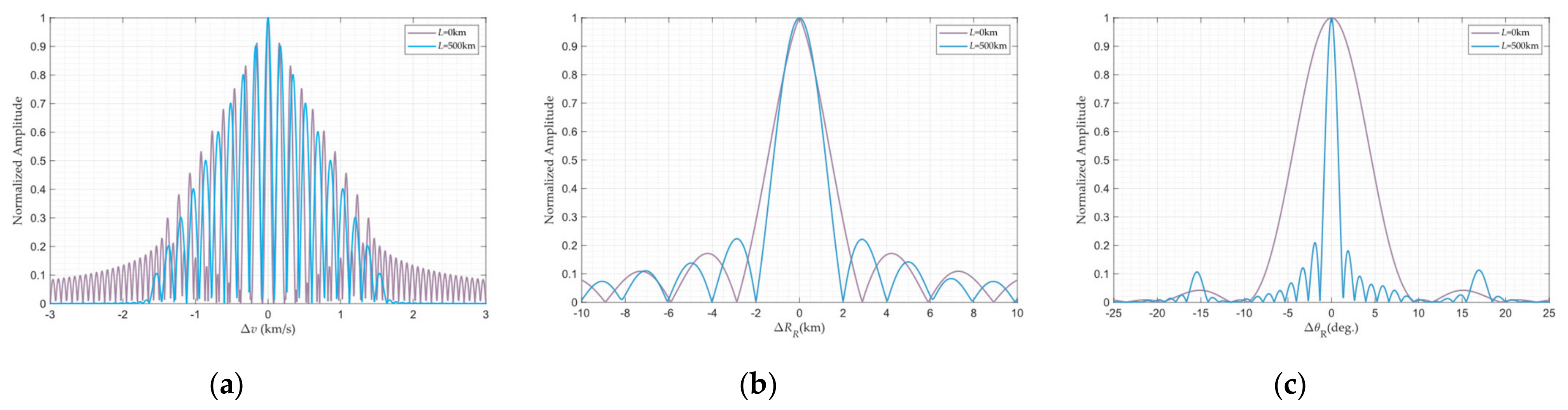
4.2.1. Velocity GAF

For this analysis, Targets 1 and 2 are modeled with the same reception distance $R_{R2}=R_{R1}=R_R$ and the same reception angle ${\theta }_{R2}={\theta }_{R1}={\theta }_R$, while their velocities differ by a distance of $\Delta v=v_2-v_1$. We analyze their dependence on diverse bistatic triangle geometries. In this geometric configuration (as shown in Figure 9), where two targets are spatially collocated, their illumination vectors become identical in both transmit and receive channels, inducing indistinguishable time-delay signatures ($\Delta \tau =0$). The Doppler shifts of the two targets and the velocity GAF are presented as follows:

$$f_{d1}=2{\displaystyle \frac{f}{c}}{v}_1\sqrt{{\displaystyle \frac{1}{2}}+{\displaystyle \frac{R_R+L\sin {\theta }_R}{2\sqrt{{R_R}^2+L^2+2R_{R}L\sin {\theta }_R}}}},$$

(48)

$$f_{d2}=2{\displaystyle \frac{f}{c}}{v}_2\sqrt{{\displaystyle \frac{1}{2}}+{\displaystyle \frac{R_R+L\sin {\theta }_R}{2\sqrt{{R_R}^2+L^2+2R_{R}L\sin {\theta }_R}}}},$$

(49)

$${\chi }_{\Delta v}\left({\mathrm{\Theta }}_1,{\mathrm{\Theta }}_2\right)=a_r^H\left({\theta }_R\right)a_r\left({\theta }_R\right)a_t^H\left({\theta }_T\right)\chi a_t\left({\theta }_T\right).$$

(50)

We sequentially vary parameters $L$, $R_{R1}$, and ${\theta }_{R1}$ (Case 1–Case 9 in Table 2) in controlled numerical simulations to investigate their individual impacts on the ambiguity function of bistatic FDA radar systems. Figure 10 displays the corresponding ambiguity functions under different bistatic configurations. It can be illustrated more clearly that all cases reach their peaks ambiguity at $\Delta v=0$ and exhibit severe velocity ambiguity and periodic spikes. This phenomenon is attributed to the fundamental characteristic of FDA’s multifrequency transmission, similar to that observed in monostatic FDA radar, rather than bistatic geometry. Concerning the impact of the geometric properties, parametric variations minimally affect main lobe properties but induce side lobe broadening: excessive baseline length $L$, short target–receiver distances $R_{R1}$, and reception angle ${\theta }_{R1}$ demonstrably degrade velocity resolution performance.

4.2.2. Range GAF

In the given configuration, Targets 1 and 2 maintain identical velocities $v_1=v_2=v$ and reception angle ${\theta }_{R2}={\theta }_{R1}={\theta }_R$ with a differential reception range of $\Delta R_R=R_{R2}-R_{R1}$ (as is shown in Figure 11). Under this configuration, Target 1 and Target 2 share identical reception angles and velocities. The differential target–receiver distance between them not only induces time-delay disparity ($\Delta \tau$) in echo signals but also creates geometric discrepancies in their bistatic triangle configurations, thereby generating transmission angles and Doppler shifts discrepancies. $\Delta \tau$, $f_{d1}$, $f_{d2}$, and the range GAF of the bistatic FDA radar can consequently be expressed as

$$\Delta \tau ={\displaystyle \frac{\left(R_{R2}+R_{T2}\right)-\left(R_{R1}+R_{T1}\right)}{c}},$$

(51)

$$f_{d1}=2{\displaystyle \frac{f}{c}}v\sqrt{{\displaystyle \frac{1}{2}}+{\displaystyle \frac{R_{R1}+L\sin {\theta }_R}{2\sqrt{R_{R1}^2+L^2+2R_{R1}L\sin {\theta }_R}}}},$$

(52)

$$f_{d2}=2{\displaystyle \frac{f}{c}}v\sqrt{{\displaystyle \frac{1}{2}}+{\displaystyle \frac{R_{R2}+L\sin {\theta }_R}{2\sqrt{R_{R2}^2+L^2+2R_{R2}L\sin {\theta }_R}}}},$$

(53)

$${\chi }_{\Delta R_R}\left({\mathrm{\Theta }}_1,{\mathrm{\Theta }}_2\right)=a_r^H\left({\theta }_R\right)a_r\left({\theta }_R\right){\left[a_t\left({\theta }_{T1}\right)\odot g^{*}\left(\Delta \tau \right)\right]}^H\chi a_t\left({\theta }_{T2}\right).$$

(54)

Numerical simulations encompassing Cases 1–9 in Table 2 yield the range ambiguity functions depicted in Figure 12. These results demonstrate that under all bistatic configurations, the ambiguity function peaks at $\Delta R_R=0$ and exhibits approximately identical main lobe structure, which is physically consistent. In contrast to velocity ambiguity functions, the bistatic FDA radar demonstrates superior inherent range resolution through the complete absence of range ambiguities and periodic side lobes, while parametrically inducing main lobe broadening—observed when extending baseline length $L$, reducing either target–receiver distance $R_{R1}$ or reception angle ${\theta }_{R1}$, accompanied by corresponding distortions in ambiguity function characteristics.

4.2.3. Angle GAF

Under these specified conditions, both targets possess velocity $v_1=v_2=v$ and reception distance $R_{R1}=R_{R2}=R_R$, coupled with an angular separation $\Delta {\theta }_R={\theta }_{R2}-{\theta }_{R1}$ in their received signals (as is shown in Figure 13). Under invariant receiver–target distances and velocities, we investigate the angular ambiguity function by systematically varying reception angles. Analogous to the range parameter study in previous sections, angular disparity between Targets 1 and 2 induces structural variations in the bistatic triangle, resulting in distinct transmission angles, temporal delay discrepancies, and Doppler shifts between the two targets. The corresponding expression of $\Delta \tau$, $f_{d1}$, $f_{d2}$, and ambiguity function is formulated as

$$\Delta \tau ={\displaystyle \frac{\left(R_R+R_{T2}\right)-\left(R_R+R_{T1}\right)}{c}},$$

(55)

$$f_{d1}=2{\displaystyle \frac{f}{c}}v\sqrt{{\displaystyle \frac{1}{2}}+{\displaystyle \frac{R_R+L\sin {\theta }_{R1}}{2\sqrt{R_R^2+L^2+2R_{R}L\sin {\theta }_{R1}}}}},$$

(56)

$$f_{d2}=2{\displaystyle \frac{f}{c}}v\sqrt{{\displaystyle \frac{1}{2}}+{\displaystyle \frac{R_R+L\sin {\theta }_{R2}}{2\sqrt{R_R^2+L^2+2R_{R}L\sin {\theta }_{R2}}}}},$$

(57)

$${\chi }_{\Delta {\theta }_R}\left({\mathrm{\Theta }}_1,{\mathrm{\Theta }}_2\right)=a_r^H\left({\theta }_{R2}\right)a_r\left({\theta }_{R2}\right){\left[a_t\left({\theta }_{T1}\right)\odot g^{*}\left(\Delta \tau \right)\right]}^H\chi a_t\left({\theta }_{T2}\right).$$

(58)

Numerical simulations employing the parametric configurations in Table 2 yield the angular ambiguity functions illustrated in Figure 14. Angular ambiguity functions exhibit similar morphological characteristics to their range–domain counterparts, attaining peak values at $\Delta {\theta }_R=0$ without discernible periodic artifacts or angular ambiguities. Notably, however, the angular ambiguity function demonstrates distinct characteristics: A narrower main lobe accompanied by side lobes, whose spatial and amplitude relationships follow an inverse proportionality with the main lobe width. Specifically, (I) a narrower main lobe correlates with side lobes positioned closer to the main lobe and exhibiting higher amplitudes, while (II) a broader main lobe results in side lobes displaced farther from the main lobe with diminished amplitudes or complete suppression. Variations in the bistatic triangular geometry simultaneously modulate both the main lobe width and side lobe characteristics. Increases in baseline length $L$ and target–receiver distances $R_R$, combined with smaller reception angles ${\theta }_R$, produce a narrower main lobe accompanied by elevated side lobe amplitudes concentrated near the main lobe. Conversely, reductions in $L$, $R_R$ or increases in ${\theta }_R$ broaden the main lobe while displacing side lobes outward with progressively decreasing amplitudes until their eventual extinction. Furthermore, the analysis reveals a critical threshold behavior: when the main lobe narrows beyond a specific width, geometric modifications exhibit diminishing returns on main lobe compression, indicating a saturation effect in angular resolution enhancement.

The above numerical simulations in Subsection 4.1 and Subsection 4.2 show that both the FDA radar’s transmitted signal and the bistatic radar’s geometric structure affect the GAF of bistatic FDA radar. Different baseband waveforms and frequency offsets of the transmitted signal significantly change the GAF’s shape. Using random frequency offsets can eliminate the synchronous linear growth of inter-element spacing and frequency offset, yielding a more ideal spiky ambiguity function. Once the transmitted signal’s baseband waveform and frequency offset are fixed, the GAF’s basic shape is set. Changes in the bistatic baseline length and target position only modify the GAF based on this basic shape, such as broadening or narrowing the main lobe and increasing or eliminating side lobes, but do not fundamentally improve the GAF. Therefore, in the design of bistatic FDA radar, the design of the baseband waveform and the selection of the frequency offset should be emphasized, while also considering the bistatic geometric configuration to achieve the best results.

Furthermore, the numerical simulations in Subsection 4.2 demonstrate the robustness of the GAF computation methodology for bistatic FDA radar in practical implementations. While actual bistatic radar deployments inevitably introduce baseline length errors and target parameter measurement inaccuracies—both contributing to minor structural deviations—the experimental results reveal that kilometer-level variations in baseline length or target positioning are required to induce changes in GAF. Practical deployment errors and target localization uncertainties orders of magnitude below this threshold. Consequently, the proposed method maintains precise characterization of bistatic FDA radar GAF and resolution performance despite these error sources, confirming its computational robustness.

4.3. Differences from Monostatic FDA Radar GAF

This subsection comparatively examines the distinctions between bistatic and monostatic FDA radar GAF. The monostatic configuration, characterized by collocated transmitter and receiver placement, eliminates bistatic geometric relationships. Consequently, targets exhibit identical transmit/receive angles, and their Doppler shifts are also no longer affected by the bistatic baseline and the position of the targets.

With Target 1’s reception angle set to 0° and all other parameters maintained consistent with the preceding simulation configuration, the GAF profiles for monostatic and bistatic FDA radar ($L=500\mathrm{km}$) at the same area are illustrated in Figure 15 and Figure 16, respectively. Figure 17 further provides comparative GAF profiles between monostatic and bistatic configurations across velocity, range, and angle dimensions. At the same time, the observed distinction between monostatic and bistatic FDA radar GAFs is also a reflection of the differences between the algorithm proposed in this paper and the baseline algorithm.

The simulation results reveal that while the GAF profiles of monostatic and bistatic FDA radar exhibit overall shape similarity, distinct disparities persist. In the angle–range GAF profiles, monostatic configuration demonstrates superior symmetry, whereas the bistatic system preserves strict symmetry only within the main lobe and first side lobe regions (refer to Figure 14 and Figure 17c), with a notable side lobe emerging at 90°—indicating symmetry breakdown when targets align with the bistatic baseline. Similarly, in the angle–rang GAF profiles, monostatic FDA radar clearly manifests the characteristic range–angle coupling of FDA waveforms with a distinct sharp peak. Bistatic FDA radars, though retaining partial coupling features (see Figure 8), exhibit weakened coupling effects due to geometric decoupling inherent in bistatic configurations.

Figure 17 provides enhanced visualization of three-dimensional GAF comparisons between monostatic and bistatic FDA radar. The two systems demonstrate marginal discrepancies in the range dimension, with the bistatic configuration exhibiting a slightly narrower main lobe. In the velocity dimension, while both systems maintain congruent global profiles, the bistatic GAF achieves nullification at a reduced threshold compared with its monostatic counterpart. Most notably within the angular dimension, the bistatic GAF exhibits a tangibly narrower main lobe, with consequentially superior angular resolution performance, attributable to spatial diversity gain inherent in bistatic geometries.

5. Conclusions

This paper explores the GAF of bistatic FDA radar. Based on conventional radar ambiguity functions and monostatic FDA radar’s GAF, a framework for bistatic FDA radar’s GAF is established, with its mathematical model derived in detail. The GAF incorporates time delay and Doppler shift, which include bistatic radar’s geometric factors, indicating the impact of bistatic radar geometry. Numerical simulations are then conducted to analyze the effects of the transmitted signal’s baseband waveform, frequency shift of FDA radar, and bistatic radar’s triangular geometry (determined by baseline length and target position) on the GAF. Results show that in bistatic FDA radar, the transmitted signal waveform design, frequency offset selection, and bistatic radar’s geometric configuration all influence the GAF, thereby affecting the radar’s velocity, range, and angle resolution. This study lays a foundation for future research and design of bistatic FDA radar systems.

Building upon the theoretical framework established in this work, our subsequent research endeavors will focus on advancing bistatic FDA radar architectures. This includes subarray solution for GAF computational complexity in real-world deployment scenarios of bistatic FDA radar, receiver structure design [27], receiver–transmitter optimization [28], and target parameter estimation and localization technology [29,30]. Furthermore, we intend to expand our research scope to encompass emerging domains such as dynamic resource allocation in dual-function radar and communication (DFRC) networks [31] and joint radar and communication (JRC) systems [32,33], direction-of-arrival (DOA) estimation and 2D direction finding [34], cognitive-MIMO-radar-related research [35], and so on.

References

- Jackson, M. The geometry of bistatic radar systems. IEE Proc. F (Commun. Radar Signal Process.) 1986, 133, 604–612. [Google Scholar] [CrossRef]
- Willis, N.J. Bistatic Radar; SciTech Publishing: Raleigh, NC, USA, 2005; Volume 2. [Google Scholar]
- Cherniakov, M. Bistatic Radar: Emerging Technology; John Wiley & Sons: Hoboken, NJ, USA, 2008. [Google Scholar]
- Wang, Y.; Luo, H.; Shao, Y.; Wang, H.; Liu, T.; Wang, Z.; Liu, K.Y.; Su, X.; Xu, H.X. Detection and Anti-Detection with Microwave-Infrared Compatible Camouflage Using Asymmetric Composite Metasurface. Adv. Sci. 2024, 11, 2410364. [Google Scholar] [CrossRef] [PubMed]
- Willis, N.J.; Griffiths, H.D. Advances in Bistatic Radar; SciTech Publishing: Raleigh, NC, USA, 2007; Volume 2. [Google Scholar]
- Kesheng, L. An analysis of some problems of bistatic and multistatic radars. In Proceedings of the 2003 Proceedings of the International Conference on Radar (IEEE Cat. No. 03EX695), Adelaide, Australia, 3–5 September 2003; pp. 429–432. [Google Scholar]
- Yulin, H.; Jianyu, Y.; Jintao, X. Synchronization technology of bistatic radar system. In Proceedings of the 2006 International Conference on Communications, Circuits and Systems, Guilin, China, 25–28 June 2006; pp. 2219–2221. [Google Scholar]
- Fang, P.; Jizhang, Z.; Yufeng, C. A Method of Time and Frequency Synchronizati on Based on Beidou Satellite for Bistatic Radar. J. Proj. Rocket. Missiles Guid. 2007, 27, 18–20. [Google Scholar]
- Geudtner, D.; Zink, M.; Gierull, C.; Shaffer, S. Interferometric alignment of the X-SAR antenna system on the space shuttle radar topography mission. IEEE Trans. Geosci. Remote Sens. 2002, 40, 995–1006. [Google Scholar] [CrossRef]
- Hanle, E. Survey of bistatic and multistatic radar. IEE Proc. F (Commun. Radar Signal Process.) 1986, 133, 587–595. [Google Scholar] [CrossRef]
- Purdy, D.S. Receiver antenna scan rate requirements needed to implement pulse chasing in a bistatic radar receiver. IEEE Trans. Aerosp. Electron. Syst. 2002, 37, 285–288. [Google Scholar] [CrossRef]
- Moyer, L.; Purdy, D. Comments on Receiver antenna scan rate requirements needed to implement pulse chasing in a bistatic radar receiver. IEEE Trans. Aerosp. Electron. Syst. 2002, 38, 300–301. [Google Scholar] [CrossRef]
- Matsuda, S.; Hashiguchi, H.; Fukao, S. A study on multibeam pulse chasing for bistatic radar. Electron. Commun. Jpn. (Part I Commun.) 2006, 89, 11–21. [Google Scholar] [CrossRef]
- Cox, P.B.; van Rossum, W.L. Analysing multibeam, cooperative, ground based radar in a bistatic configuration. In Proceedings of the 2020 IEEE International Radar Conference (RADAR), Washington, DC, USA, 28–30 April 2020; pp. 912–917. [Google Scholar]
- Antonik, P.; Wicks, M.C.; Griffiths, H.D.; Baker, C.J. Frequency diverse array radars. In Proceedings of the 2006 IEEE Conference on Radar, Verona, NY, USA, 24–27 April 2006; p. 3. [Google Scholar]
- Secmen, M.; Demir, S.; Hizal, A.; Eker, T. Frequency diverse array antenna with periodic time modulated pattern in range and angle. In Proceedings of the 2007 IEEE Radar Conference, Waltham, MA, USA, 17–20 April 2007; pp. 427–430. [Google Scholar]
- Huang, J.; Tong, K.-F.; Baker, C. Frequency diverse array with beam scanning feature. In Proceedings of the 2008 IEEE Antennas and Propagation Society International Symposium, San Diego, CA, USA, 5–11 July 2008; pp. 1–4. [Google Scholar]
- Tan, M.; Wang, C.; Li, Z. Correction analysis of frequency diverse array radar about time. IEEE Trans. Antennas Propag. 2020, 69, 834–847. [Google Scholar] [CrossRef]
- Rothstein, J. Probability and Information Theory, with Applications to Radar. PM Woodward. McGraw-Hill, New York; Pergamon Press, London, 1953. 128 pp. Illus. $4.50. Science 1954, 119, 874. [Google Scholar] [CrossRef]
- San Antonio, G.; Fuhrmann, D.R.; Robey, F.C. MIMO radar ambiguity functions. IEEE J. Sel. Top. Signal Process. 2007, 1, 167–177. [Google Scholar] [CrossRef]
- Celik, O.O.; Tuncer, T.E. MIMO radar beampattern design by using Phased-Costas waveforms with PAR constraints employing a generalized ambiguity function. Digit. Signal Process. 2023, 135, 103948. [Google Scholar] [CrossRef]
- Chen, Z.; Liang, J.; Song, K.; Yang, Y.; Deng, X. On designing good doppler tolerance waveform with low PSL of ambiguity function. Signal Process. 2023, 210, 109075. [Google Scholar] [CrossRef]
- Wang, W.-Q.; Dai, M.; Zheng, Z. FDA radar ambiguity function characteristics analysis and optimization. IEEE Trans. Aerosp. Electron. Syst. 2017, 54, 1368–1380. [Google Scholar] [CrossRef]
- Gui, R.; Huang, B.; Wang, W.-Q.; Sun, Y. Generalized ambiguity function for FDA radar joint range, angle and Doppler resolution evaluation. IEEE Geosci. Remote Sens. Lett. 2020, 19, 1–5. [Google Scholar] [CrossRef]
- Tsao, T.; Slamani, M.; Varshney, P.; Weiner, D.; Schwarzlander, H.; Borek, S. Ambiguity function for a bistatic radar. IEEE Trans. Aerosp. Electron. Syst. 1997, 33, 1041–1051. [Google Scholar] [CrossRef]
- Chen, H.-W.; Li, X.; Yang, J.; Zhou, W.; Zhuang, Z. Effects of geometry configurations on ambiguity properties for bistatic MIMO radar. Prog. Electromagn. Res. B 2011, 30, 117–133. [Google Scholar] [CrossRef]
- Xu, J.; Zhang, Y.; Liao, G.; Xu, Y.; Wang, W. Angle-Dependent Matched Filtering for Moving Target Indication With Coherent FDA Radar. IEEE Trans. Aerosp. Electron. Syst. 2024, 60, 3523–3536. [Google Scholar] [CrossRef]
- Lan, L.; Rosamilia, M.; Aubry, A.; De Maio, A.; Liao, G. FDA-MIMO transmitter and receiver optimization. IEEE Trans. Signal Process. 2024, 72, 1576–1589. [Google Scholar] [CrossRef]
- Hyder, M.M.; Mahata, K.; Hasan, S.M. A new target localization method for bistatic FDA radar. Digit. Signal Process. 2021, 108, 102902. [Google Scholar] [CrossRef]
- Fang, Y.; Zhu, S.; Liao, B.; Li, X.; Liao, G. Target Localization With Bistatic MIMO and FDA-MIMO Dual-Mode Radar. IEEE Trans. Aerosp. Electron. Syst. 2024, 60, 952–964. [Google Scholar] [CrossRef]
- Zhang, H.; Liu, W.; Zhang, Q.; Zhang, L.; Liu, B.; Xu, H.-X. Joint Power, Bandwidth, and Subchannel Allocation in a UAV-Assisted DFRC Network. IEEE Internet Things J. 2025, 12, 11633–11651. [Google Scholar] [CrossRef]
- Zhang, H.; Liu, W.; Zhang, Q.; Liu, B. Joint customer assignment, power allocation, and subchannel allocation in a UAV-based joint radar and communication network. IEEE Internet Things J. 2024, 11, 29643–29660. [Google Scholar] [CrossRef]
- Zhang, H.; Weijian, L.; Zhang, Q.; Taiyong, F. A robust joint frequency spectrum and power allocation strategy in a coexisting radar and communication system. Chin. J. Aeronaut. 2024, 37, 393–409. [Google Scholar] [CrossRef]
- Wang, X.; Guo, Y.; Wen, F.; He, J.; Truong, T.-K. EMVS-MIMO radar with sparse Rx geometry: Tensor modeling and 2-D direction finding. IEEE Trans. Aerosp. Electron. Syst. 2023, 59, 8062–8075. [Google Scholar] [CrossRef]
- Qi, C.; Xie, J.; Zhang, H.; Liu, W.; Feng, W.; Zheng, G. Optimizing low-grazing angle detection for maneuvering targets in cognitive MIMO radar networks: A shapley value approach. IEEE Trans. Veh. Technol. 2024, 74, 4977–4992. [Google Scholar] [CrossRef]