Abstract
Highly accurate data on urban and rural settlement (URS) are essential for urban planning and decision-making in response to climate and environmental changes. This study developed an optimal random forest classification model for URSs based on spectral–topographic–radar polarization features using Landsat 8, NASA DEM, and Sentinel-1 SAR as the remote-sensing data sources. An optimal urban and rural settlement boundary (URSB) extraction technique based on morphological and pixel-level statistical methods was established to link discontinuous URSs and improve the accuracy of URSB extraction. An optimal random forest classification model for URSs was developed, as well as a technique to optimize URSB, using the Google Earth Engine (GEE) platform. The URSB of Xining, China, in 2020 was then extracted at a spatial resolution of 30 m, achieving an overall accuracy and Kappa coefficient of 96.21% and 0.92, respectively. Compared to using a single spectral feature, these corresponding metrics improved by 16.21% and 0.35, respectively. This research also demonstrated that the newly constructed Blue Roof Index (BRI), with enhanced blue roof features, is highly indicative of URSs and that the URSB was best extracted when the window size of the structural elements was 13 × 13. These results can be used to provide technical support for obtaining highly accurate information on URSs.
1. Introduction
Urban and rural settlements (URSs) refer to areas where urban cities and rural regions congregate, characterized by high levels of human activities [1]. In the past few decades, human-occupied land has expanded rapidly, and a large amount of natural land has been covered by impervious surfaces [2]. Research has shown that land-use/-cover change, mainly in URSs, is the most dramatic and irreversible land-use transformation affecting Earth’s ecosystems [3], with important implications for biogeochemical cycling [4], hydrological processes [5], climate change [6], and biodiversity [7] at the local, regional, and global scales. For example, the disorderly expansion of cities has led to the loss of a large amount of high-quality cultivated land, the deforestation of large tracts of forests, and the overexploitation of natural resources, which has deteriorated the ecological environment, posing considerable challenges to the sustainable development of cities [8]. Timely and accurate urban and rural settlement boundaries (URSBs) are the basis of urban planning and environmental protection.
The extraction of URSBs using the manual interpretation and field survey data is highly dependent on the subjective experience of the interpreter. In addition, it is inefficient, time-consuming, and unsuitable for large-scale, dynamic, and rapid automated extractions [9]. Currently, the primary methods for extracting urban boundaries from remote-sensing images include threshold, mutation detection, and clustering methods. The threshold methods are simple, fast, and have good results at local scales [10,11,12]—for example, the Normalized Difference Built-Up Index (NDBI) [13] and the Index-based Built-Up Index (IBI) [14]. However, determining this threshold is both subjective and empirical. Mutation detection is essentially a dynamic threshold method. By automatically detecting the mutation points of different land-use types, this method can effectively differentiate urban and rural areas and even urban–rural fringe areas; however, it cannot determine precise boundaries [15,16,17]. The clustering method aggregates similar data and has been widely used in urban boundary extraction, such as global [9,18] and Chinese urban boundaries [19]. Nevertheless, even though the clustering method can effectively extract the main range of urban and rural areas from remote-sensing images, the extraction of boundaries is inaccurate. In spite of the capability of optical remote-sensing images (such as Landsat, Sentinel 2A, etc.) to capture the reflection characteristics of the surface of ground objects, it is challenging to distinguish URSs from land uses with similar spectral characteristics from bare soil, sand, and gravel [20]. Synthetic aperture radar (SAR) data, such as Sentinel-1A, can provide detailed information on surface structural characteristics and dielectric properties of ground objects but are affected by complex terrain and shadows [2]. Nighttime light remote-sensing data have been proven to be effective in identifying relatively active urban areas, but they ignore settlements such as rural areas and small towns, resulting in an underestimation of URSs [21], and the spatial resolution of nighttime light data is low, making it challenging to obtain high-accuracy boundaries.
With the continuous increase in open-source remote-sensing data, multi-source datasets were used to extract URSs [22], namely the following: The China physical urban boundary (CPUB) based on Landsat data, nighttime light data, and OpenStreetMap road data [16]; a dataset of urban built-up areas in China (abbreviated as DUBC) based on nighttime light data, the normalized difference vegetation index (NDVI), and land surface temperature (LST) [23]; and global city boundary products based on Landsat images, Sentinel images, and population data (greater than 1500 people per square kilometer) [24]. Although these boundary products have a high degree of consistency in the main urban areas, they are less accurate in suburban and rural areas. In particular, the extraction accuracy of the plateau URSBs with complex terrains and particular climates is low.
This study aims to use Landsat 8, NASA DEM, and Sentinel-1 SAR as remote-sensing data sources to develop an optimal random forest classification model based on spectral–topographic–synthetic aperture radar (SAR) polarization features of URSs. Using this model, this study aims to establish an optimized URSB technology based on morphology and pixel statistical methods combined with the Google Earth Engine (GEE) platform to conduct URSB extraction with a 30 m spatial resolution and fast and accurate URS mapping in plateau areas in Xining, China, in 2020.
2. Study Area and Data
2.1. Study Area
Xining is the capital city of Qinghai Province, China, located in the northeastern part of the Qinghai-Tibetan Plateau between the northern and southern mountains of the Hehuang Valley, and it is the largest city on the Qinghai-Tibetan Plateau. Xining is located at 100°58′48″E~102°01′26″E and 36°24′40″N~37°03′33″N, with the highest and lowest elevations being 4863 m and 2160 m, respectively (Figure 1). This city has a complex topography and a continental-plateau semi-arid climate [25]. Owing to terrain constraints, the urban areas of Xining City are primarily concentrated in the central flat areas of the river valleys, while rural areas are linearly distributed along the valleys. Most areas on both sides of the valleys consist of steep slopes that are mainly used for agriculture, with some patches of bare land.
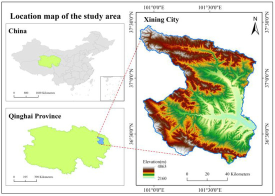
Figure 1.
Geographic location and topography of the study area.
2.2. Data Sources and Preprocessing
2.2.1. Landsat 8 Surface Reflectance (SR) Imagery
All remote-sensing image calling and preprocessing operations were performed using the GEE. This study used Landsat 8 SR imagery as an optical remote-sensing data source with a spatial resolution of 30 m and a temporal resolution of 16 days.
Xining experiences frequent cloud cover throughout the year. This makes it challenging to obtain single-time-phase high-quality satellite imagery and requires the cloud filtering of raw data and image composites. Cloud filtering was conducted by screening images with less than 20% cloud cover in 2020, totaling 44 scenes. The ‘pixel_qa’ band was used to filter out cloudy pixels, analyze the number of overlapping images and availability of each pixel, and identify effective pixels that could cover the entirety of Xining City (Figure 2). Image compositing employed the median compositing algorithm in the GEE to generate a cloud-free, high-quality remote-sensing image from the 44 acquired scenes.
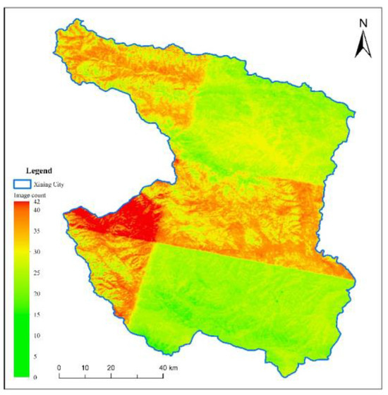
Figure 2.
Number of cloud-free images corresponding to each pixel in Xining, 2020.
2.2.2. Sentinel-1 SAR Data
The Sentinel-1A satellite carries a C-band synthetic aperture radar (SAR) that operates regardless of weather conditions [26]. In this study, the Interferometric Wide swath (IW) imaging mode was selected to obtain 2020 SAR images by median compositing all SAR data collected from 1 January 2020 to 31 December 2020. The VV and VH SAR polarization features in combination with dual-band cross-polarization were extracted. VV represents the transmission in the vertical direction and reception in the vertical direction, and VH represents the transmission in the vertical direction and reception in the horizontal direction. Sentinel-1 images were resampled to 30 m.
2.2.3. DEM Data
The NASA Digital Elevation Model (DEM) used in this study was generated by improved reprocessing based on Shuttle Radar Topography Mission (SRTM) data, which provides higher accuracy and broader coverage with a spatial resolution of 1 arcsec (~30 m) than the SRTM DEM [27].
2.2.4. Validation Data
In this study, Google Earth high-resolution imagery (spatial resolution of 0.6 m) and four existing urban boundary products (GUB2020 [9], CPUA2020 [28], GHS-SMOD2020 [29], and the dataset of urban built-up area in China in 2020 (DUBC2020) [23]) were used to validate the accuracy of the boundaries.
3. Research Methodology
3.1. Methodology Overview
The extraction of URSBs consists of five main steps (Figure 3): (1) Preprocessing: Included cloud filtering, resampling, and image median compositing; (2) Feature extraction: Spectral features, topographic features, and SAR polarization features were extracted from multi-source remote-sensing images; (3) Optimal random forest model construction: Mainly included calculating the optimal decision-tree parameters and optimal feature indicators; (4) Random forest classification and accuracy evaluation; and (5) Drawing the boundary: The result with the highest classification accuracy was selected, the boundary of the URS was drawn using the morphological algorithm and eight-neighborhood pixel statistics, and the vector boundary information was extracted using the edge detection algorithm.
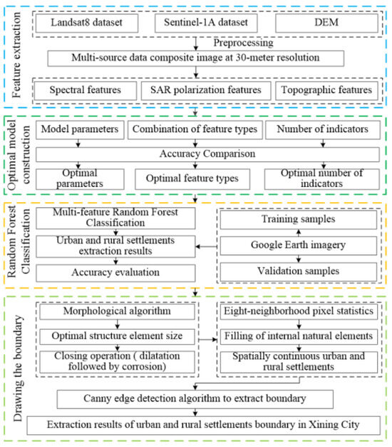
Figure 3.
Overall flow chart of URSB extraction.
3.2. Feature Construction
The selected URS features include spectral, topographic, and SAR polarization features. Twenty-four feature coefficients were constructed (Table 1), which are described below:

Table 1.
Features extracted from urban and rural settlements.
3.2.1. Spectral Features
Spectral features were selected, including the original spectral bands, tasseled cap transformation features, and spectral indices. The spectral bands used were B2, B3, B4, B5, B6, B7, and B10, with a total of seven bands. Tasseled cap transformation is a linear transformation based on multispectral bands that eliminates the relative spectral correlation of multispectral images and is widely used in urban land classification [30,31]. Landsat 8 multispectral imagery was transformed to obtain three feature indicators: greenness, brightness, and wetness.
Spectral indices can further characterize target information. Research shows that NDBI [13], NDISI [32], ENDISI [33], and IBI [14] values can effectively enhance URS information and improve recognition accuracy and the classification effect. The MNDWI [34] index and four vegetation indices (NDVI [35], EVI [36], RVI [37], and DVI [38]) were selected to extract non-URS features such as water, ice, snow, and vegetation information. In general, these spectral indices are selected to make full use of spectral information in different bands and enhance the information of the URS and other ground objects, thereby achieving an effective extraction and analysis of URS information.
Since there are many blue-based high-reflectivity buildings in Xining’s urban and rural areas, it is necessary to enhance the features of such ground objects further to improve the accuracy of URS extraction. By analyzing the spectral feature curves of typical ground objects in Xining (Figure 4), it was found that the reflectance of the blue-roof building was higher in the blue band (B2) and the shortwave infrared 1 band (B6). However, the difference in the reflectances of B2 and B6 was not significantly different from that of the other features. Therefore, subtracting the two bands and dividing them by the sum of the two bands can effectively highlight the differences in the features of the blue-roof building and the rest of the ground objects. The Blue Roof Index (BRI) is calculated as follows:
where BLUE is the blue band of the Landsat 8 satellite and SWIR1 is the shortwave infrared 1 band of the Landsat 8 satellite.
BRI = (SWIR1 − BLUE)/(SWIR1 + BLUE)
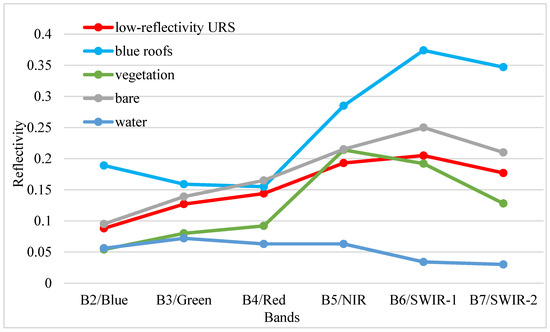
Figure 4.
Spectral features of typical ground objects in Xining.
3.2.2. Topographic Features
The overall elevation of Xining is high, and the terrain is complex and undulating, limiting URS spatial distribution [39]. Therefore, elevation and slope indicators were extracted as model feature inputs based on the generally gentle slopes and relatively low elevations of the URS.
3.2.3. SAR Polarization Features
Owing to the high dielectric properties of building material surfaces and the unique geometry of manmade structures that can produce stronger backscattered echo signals than other ground objects, SAR data can be used as a distinctive representation of URSs [40]. VV and VH polarization characteristics can better reflect the geometric characteristics of an artificial building surface [20]; therefore, both were used as SAR polarization feature input models.
3.3. Random Forest Model Generation
Random forest (RF) is a decision-tree-based machine learning algorithm that integrates the Random Subspace method and the bagging integrated learning theory [41]. The random forest algorithm has the advantages of strong robustness, high stability, and efficient data processing, which play an essential role in urban land-use monitoring [42,43,44]. Therefore, a random forest model was used for the classification in this study.
3.3.1. Construct Sample Data
The land-cover types in Xining include high- and low-reflectance urban and rural settlements, vegetation, water bodies, bare land, snow, and ice. Based on the binary classification, Xining was divided into URSs and other categories. This study utilized high-resolution imagery from Google Earth and Landsat 8 for 2020. A total of 1365 samples were uniformly selected within the study area through visual interpretation. Using a nearly 1:1 random split, the samples were divided into 705 training and 660 validation samples (Table 2).
Table 2.
Number of samples for remote-sensing classification of URS.
3.3.2. Selection of Model Parameters
The performance of the random forest model is primarily affected by two parameters: the number of random forest decision trees (N) and the number of features that can be selected for each decision-tree node (M). This model was primarily used for classification in this study, and M can be set directly to the default value, which is the square root of the number of input features [45]. The number of decision trees (N) directly affects the classification accuracy; too small a value of N is easy to underfit, and too large a value increases the computing time and reduces computing efficiency. Therefore, the relationship between N and accuracy must be further explored to obtain the optimal model parameters. For this purpose, iterations were run from 5 to 200, with 5 as the number of tree intervals. As the number of trees (N) increased, the overall accuracy gradually improved, and the optimal model parameters were obtained by taking N as the maximum overall accuracy. The other model parameters were set to default values.
3.3.3. Optimization of Input Features
Differences in the features of typical ground objects are a prerequisite and key to classification. Therefore, selecting appropriate feature indicators is very important for the classification of ground objects. In this study, different indicators were extracted to describe the URS from multiple dimensions based on the different features exhibited by the URS in multi-source remote-sensing datasets. To obtain optimal feature indicators, multi-feature-type combination experiments were designed to analyze the differences in the results under different feature-type combinations from both qualitative and quantitative aspects.
After obtaining the best combination of feature types, the number of indicators still requires optimization because not all indicators have the same importance in classification, and too many indicators will reduce the efficiency of the classification model and affect the accuracy of the classification, resulting in ‘dimension disaster’ [46]. Therefore, we used the importance analysis method of the GEE platform, i.e., the ‘explain ()’ method in the classifier, to calculate the average contribution of each input feature in the classification of the random forest model and select the optimal feature indicators by ranking them.
Therefore, this study designed four sets of experiments to analyze the effects of different combinations of feature indicators on the classification results and verify the necessity of feature type combinations. Experiment I: spectral features only; Experiment II: spectral features + topographic features; Experiment III: spectral features + SAR polarization features; and Experiment IV: spectral features + topographic features + SAR polarization features. Based on determining the spectral, topographic, and polarization characteristics as the best feature combination, the number of indicators was further screened according to their importance in the classification.
3.3.4. Evaluation of Extraction Accuracy
Accuracy evaluation is the assessment of the accuracy of remote-sensing classification results, and the quality of the classification results can be directly judged by comparing the classification results with sample points of known attributes. Currently, the accuracy evaluation system widely used in the field of land-use/-cover monitoring is the confusion matrix evaluation system, and the central evaluation indicators include the overall accuracy, the Kappa coefficient, user accuracy, and producer accuracy [47].
3.4. Boundary Extraction
The URS obtained after classification using the random forest model is typically spatially discontinuous and tends to have multiple closed areas. For example, there are natural spaces such as water bodies and green spaces of varying sizes within the city, and there is no clear and complete boundary in the fringe areas of the city as the density of buildings decreases and the degree of fragmentation increases. The presence of background ground objects such as bare land and vegetation between neighboring houses in rural areas also leads to spatial discontinuity. To automatically and accurately extract the boundaries of URSs, this study designed the following three steps based on the GEE (Figure 5): First, boundary delineation based on morphology—that is, the spatial aggregation of URS classification results and delineation of boundaries based on erosion and dilatation algorithms, as well as the removal of noise points and smoothing of edge areas (Figure 5c). Second, natural elements—that is, automatically identifying and filling in natural elements (waterbodies, green areas, etc.) within the URS to ensure spatial continuity and integrity to optimize the boundaries of the URS (Figure 5d). Third, edge detection identifies the boundary—that is, the Canny edge detection algorithm identifies and extracts the vector boundary (Figure 5e).
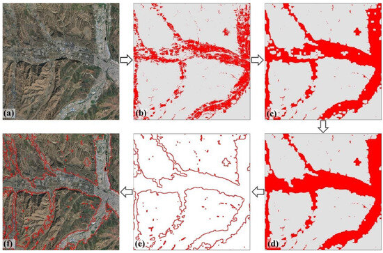
Figure 5.
URSB extraction process. (a) Google Earth remote-sensing image; (b) Random forest model classification results; (c) Morphological operations to delineate the boundary; (d) Filling in the internal natural elements; (e) Extracting the boundary; (f) Boundary results superimposed on Google Earth imagery.
3.4.1. Morphology-Based Boundary Delimitation
Morphology is a commonly used method for boundary construction [48,49], and its basic operations include erosion, dilation, and opening and closing operations [50]. This study used a combination of two common morphology operators, namely erosion and dilation, to delineate the boundaries. The purpose of connecting neighboring URS patches, filling small internal holes, and smoothing the boundaries of the marginal areas was achieved by selecting appropriately sized structural elements to perform closing operations (dilation followed by erosion) on the target image.
(1) Erosion. Erosion can be expressed as follows:
where X is the original image, B is the structural element, and x is the collection after erosion using B.
(2) Dilation. The dilation can be expressed as follows:
where X is the original image, B is the structural element, and x is the collection after dilation using B.
(3) Closing. The closing operation is a combination of erosion and dilation—that is, image X passes through structural element B and undergoes erosion followed by dilation, which can be expressed as follows:
The sizes of the structural elements determine the processing effect of the image. Therefore, the effect of this parameter on boundary extraction must be further explored to set the optimal structural elements.
3.4.2. Filling the Natural Space
After morphological closure, the small internal holes were eliminated, and a larger area of the water body and green space were further identified and extracted. The analysis revealed that, after the morphological closing operation, the results exhibited strong spatial connectivity (Figure 5c), but numerous voids remained within the urban area (natural elements). These voids exhibit a certain degree of isolation compared with urban and rural settlements, which consist of fewer pixels. Conversely, rural settlements are also encompassed by non-urban and rural settlements, showing isolation. Therefore, through image processing, all the isolated patches were extracted and merged into urban and rural settlements. It is worth noting that this was not aimed at detecting natural elements because rural settlements were also extracted.
The Connected Pixel Count (maxSize, eightConnected) function provided by the GEE can calculate the number of connected pixels within the eight neighborhoods of each pixel (objects in both the edge and corner neighborhoods); the higher the count, the larger the structure of patches with the same attribute value becomes, which are then filtered out and converted into target attributes. The operating principle is illustrated in Figure 6. First, the Connected Pixel Count (maxSize, eightConnected) function was used to filter and screen patches with smaller areas, which were typically rural buildings, water bodies, and green space elements (Figure 6b). The area threshold was determined by the maximum range parameter max size of the pixel neighborhood, which was set to a 1024-pixel range maximum, after which the attribute of all patches was modified to 1, as shown in Figure 6c. Finally, the small patch layer was superimposed on the original image to obtain the filled URS (Figure 6d).
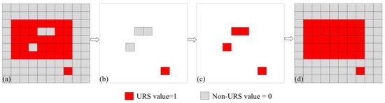
Figure 6.
Image processing for detecting isolated patches and merging URSs: (a) Initial URSs; (b) Screening small patches; (c) Converting attribute values; (d) Filled URSs.
In this process, the parameter ‘1024’ indicates the maximum distance to be considered when calculating connected pixels, meaning the count is conducted within a range of 1024 pixels. The default value for this parameter is 100; however, it was set to the maximum value accepted by the GEE, which is 1024, to broaden the retrieval range. The second parameter, ‘eightConnected’, indicates whether to use the eight-connected rule or the four-connected rule, with the default value set to true.
3.4.3. Edge Detection for Identifying Boundaries
Boundaries were extracted using the Canny edge detection algorithm provided by the GEE. Canny edge detection uses four separate filters to identify diagonal, vertical, and horizontal edges and calculates first-order derivative and gradient magnitude values in the horizontal and vertical directions [51]. Because the classification result is a binary image with attribute values of 1 (URS) and 0 (non-URS), it is only necessary to set 0 as the threshold value (above which the gradient magnitude is higher) to consider the pixel as an edge-detection object only and retain the detected edges. The detected edges are converted to vector format data by the ‘Image.reduceToVectors()’ function to obtain the final vector boundary data.
4. Results and Analysis
4.1. Number of Optimal Decision Trees for Random Forest Model
The effect of the variation in the number of decision trees on the overall accuracy is shown in Figure 7. As the number of trees (N) increased, the overall accuracy gradually increased, reaching a maximum value of approximately 96.1% when N was 55. As N continued to increase, the overall accuracy remained relatively stable. Considering that an excessive number of decision trees affected the efficiency of the model, it was set to N = 55 to balance the stability and accuracy of the model.
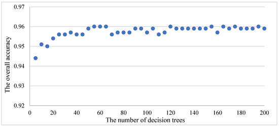
Figure 7.
Effect of different number of decision trees on the overall accuracy of the random forest model.
4.2. Selection of Optimal Indicators
4.2.1. Selection for Optimal Feature Combinations
The accuracy of the classification results for the four groups of control experiments (Table 3) showed significant variability in the extraction results for different combinations of feature types. Taking Experiment I as a reference, by adding terrain features (Experiment II), the overall accuracy, the Kappa coefficient, user accuracy, and producer accuracy were improved by 9.85%, 0.21, 10.42%, and 15.24%, respectively. By adding SAR polarization features (Experiment III), the accuracy indexes were improved by 12.42%, 0.27, 15.00%, and 18.04%, respectively. However, with the combination of the proposed multiple feature indicators (Experiment IV), compared with Experiment I, the accuracy indexes were improved by 16.21%, 0.35, 18.33%, and 25.01%, respectively. The experimental results show that including topographic and SAR polarization indicators can improve classification accuracy to different degrees. In contrast, the synergistically modeled spectral topographic SAR polarization features had the best classification accuracy.
Table 3.
Extraction accuracy with different feature combinations.
To verify the feature combination extraction effect of URSs, four typical regions were selected, representing urban areas, suburban areas, rural areas, and mountainous areas, and the extraction results of the four groups of experiments, which were obtained by combining the importance of the indicators of the four groups of experiments, were compared in detail (Figure 8). Notably, the spectral feature indicators in Experiment I used to extract the URS still had obvious classification errors. For example, the spatial distribution of rural settlements was significantly underestimated by omitting references to low-density buildings in rural areas, and the extent of the URS was overestimated by misclassifying bare land as a URS because of the similarity in spectral features between bare rock surfaces in mountainous areas, fallow agricultural land in rural areas, and the URS. In Experiment II, elevation and slope topography indicators were added to further weaken the influence of high-elevation bare rock in mountainous areas and reduce misclassifications. Unlike plains, mountain ranges and hills surround the urban area of Xining, and the high elevation and significant slope topography are inconducive to urban expansion. Therefore, topographic indicators played a vital role in the classification, with slope and elevation ranking as the top two in terms of classification importance (Figure 9). Adding SAR polarization features significantly reduced the misclassification of fallow bare land and enhanced the information on artificial structures. Compared to Experiments I and II, both URS extraction results were more accurate, with higher aggregation and fewer noise points. The VH and VV polarization indicators ranked in the top two in terms of model classification contribution (Figure 9). Nevertheless, it is still not possible to improve the separability of bare rock and target information, resulting in the misclassification of mountainous areas. Experiment IV, in which spectral, topographic, and SAR polarization features were jointly input into the model, dramatically improved the distinction between the URS and bare land and reduced the misclassification of cultivated land in rural areas and bare rock in mountainous areas. At the same time, a more complete extraction of URSs, even in low-density rural areas, reduces the phenomenon of missed classifications. The classification results of the combination of multitype feature indicators were more in line with the actual spatial distribution of the URS, and the classification effect was the best. Topography and SAR polarization indices play a significant role and rank among the top four in importance. The Blue Roof Index proposed in this study ranks fifth in importance (Figure 9) and first among all the spectral feature indices, which is essential for accurately extracting the URS.
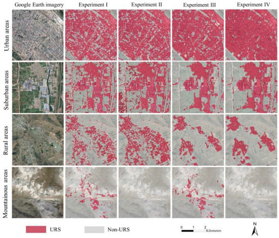
Figure 8.
Results of the classification of different types of feature indicators in typical areas.
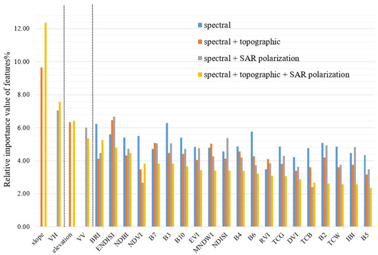
Figure 9.
Relative importance of different features in the extraction of URS.
4.2.2. Optimization of Feature Number
Based on the optimal feature combinations of spectral, topographic, and SAR polarization features (24 in total) and the relative importance values in classification (Figure 9), the first n (n ϵ [0, 24]) indicators were sequentially input to participate in the classification, and the classification accuracies were obtained separately. The overall accuracy increased with the number of indicators (Figure 10), reaching its highest accuracy at the 13th indicator. As the number of indicators continued to increase, the overall accuracy maintained a slight fluctuation at 96%. Therefore, the first 13 were selected as the final feature indicators, including 9 spectral indicators, 2 topographic feature indicators, and 2 SAR polarization feature indicators (Table 4).
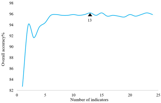
Figure 10.
Classification accuracy of different quantitative indicators.
Table 4.
Results of the optimized selection of indicators.
4.3. Identification of Morphological Structure Element Size
This study used a morphology-based closing algorithm to optimize the boundaries of the extracted URS to solve the problems of spatial fragmentation and poor connectivity of the extraction results of URSs. The size of the sliding window of a structural element is a crucial parameter for optimizing the boundary effect. Nine windows of different sizes were set up to demarcate the boundaries: 3 × 3, 5 × 5, 7 × 7, 9 × 9, 11 × 11, 13 × 13, 15 × 15, 17 × 17, and 19 × 19. The results (Figure 11) show that as the window size increased, the connectivity of the URS gradually improved, and the small internal holes gradually decreased. However, detailed boundary information is simultaneously lost, resulting in severe jaggedness. When the window size of the structural elements was 13 × 13, the connectivity of the URS was better and the boundary was smooth and continuous, which was most consistent with the actual spatial distribution.
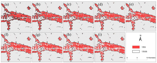
Figure 11.
Localized comparison of the results of URSB with different window sizes. The window sizes were (a) 3 × 3; (b) 5 × 5; (c) 7 × 7; (d) 9 × 9; (e) 11 × 11; (f) 13 × 13; (g) 15 × 15; (h) 17 × 17; (i) 19 × 19.
4.4. Extraction of Urban and Rural Settlements Boundary
4.4.1. Extraction of Urban and Rural Settlements
Based on the type and number of optimization indicators, the random forest model was used to map the URS in Xining in 2020 (Figure 12). The URS in Xining is distributed in the river valley basin, with the city mainly concentrated in the central and eastern valleys, which restricts rural areas; the spatial distribution is relatively decentralized, with many points, a wide range of surfaces, irregular shapes, etc. In 2020, the total URS area in Xining was 325.48 km2, accounting for approximately 4.28% of the total area of Xining. The confusion matrix accuracy validation using 660 test points showed that the overall accuracy was 96.21%, the Kappa coefficient was 0.92, producer accuracy was 97.36%, and user accuracy was 92.08%, which is a reasonable classification effect and high accuracy.
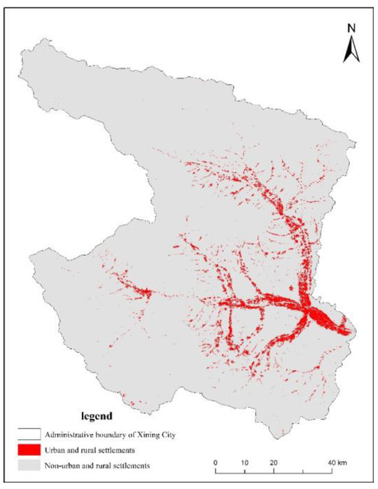
Figure 12.
Extraction of urban and rural settlements boundary.
4.4.2. Extraction of Urban and Rural Settlements Boundary
Based on the classification results of the optimal random forest model, the initial results were used to extract the final URS vector boundaries by performing morphological operations, recognizing and filling internal natural elements, and edge detection. Specifically, four levels—city, county, town (township), and village—were selected. The boundaries were superimposed onto Google Earth imagery (Figure 13). It can be clearly observed that the boundaries match the spatial extent of the actual URS, indicating that the boundaries extracted in this study can effectively separate the URS from the areas of other land-use types, and that the boundaries are continuous and complete. In high-density urban areas (Figure 13A,B), natural elements such as internal green spaces and water bodies are included completely, and the boundary details are rich in information. In rural areas (Figure 13C,D), low-density settlements were interspersed with background ground objects, but accurate boundaries with a very high match could also be extracted.
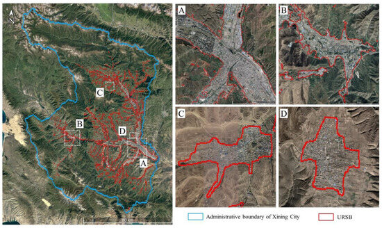
Figure 13.
Results of extracting URSB in Xining in 2020: (A) Xining; (B) Huangyuan County; (C) Jile Township; (D) Dayoushan Village.
5. Discussion
5.1. Factors Affecting Boundary Extraction Accuracy
5.1.1. Remote-Sensing Data
The spatial resolution for remote-sensing imagery should be selected based on the research objectives and application requirements. This study aimed to acquire the spatial distribution and boundary information of urban and rural residential areas. Existing research indicates that, by focusing on urban areas, a spatial resolution of 30 m (or 38 m) may be the optimal choice because it can encompass urban regions without missing too much urban information. As the image resolution increases (to 1 or 10 m), the extracted urban area may decrease because finer urban details (such as parks and vegetation) can be depicted [52]. If a detailed classification of small or complex features within urban areas, such as buildings, road networks, and green spaces, is required, higher spatial resolutions (such as Sentinel-2) are typically more suitable. Additionally, Landsat satellites have been operational since 1972, forming a decade-long time series of observational data. In future studies, emphasis should be placed on dynamic monitoring using long-term time-series data.
Obtaining high-quality optical remote-sensing images of a single seasonal time phase for plateau-type cities with severe year-round cloud pollution is more challenging. Pixel-based image compositing methods can simultaneously utilize a large amount of image data, effectively reducing the effects of cloud and aerosol contamination and filling in gaps in the dataset [53]. It has been shown that a significant improvement in the quality of annual composite images of urban areas can significantly reduce the impact of clouds and cloud shadows on mapping accuracy [54]. Moreover, the median composite is more suitable for annual dense time-series imagery, which ensures the variability of feature indicators [55]. In this study, the annual median composite method was used to obtain high-quality optical remote-sensing images from Xining in 2020 as classification data, providing high-quality data support for URSB extraction.
5.1.2. Feature Indicators of Multi-Source Datasets
Because of the spectral heterogeneity of URSs, it is difficult to accurately extract URS using only spectral features, and using multi-source datasets can effectively improve their mapping accuracy [56]. In this study, the recognition accuracy of URSs was improved by combining multi-source datasets to extract different types of feature indicators (spectral, topographic, and SAR polarization features) as training input indicators for the random forest model. The results (Figure 9) showed that topographic features (slope and elevation) contributed the most to the final decision. This is because human settlements are usually located in relatively flat areas, especially in plateau cities where the topography is complex, which increases the importance of topographic features [20]. It has been shown that topographic variables significantly contribute to urban mapping in mountainous areas [57]. Meanwhile, SAR polarization features (VH and VV) also help improve the recognition accuracy of URSBs because SAR images can obtain information about the special structural and dielectric properties of artificial objects. The SAR polarization characteristics can effectively distinguish URSs from bare soil (such as fallow farmland) with similar spectral characteristics. Nevertheless, similar backscatter signals are found in mountainous areas compared to urban areas, leading to the misidentification of some bare rocks as URSs, which can address the introduction of topographic features [58]. The final indicator in the importance ranking was the spectral features, which included three building indices (BRI, ENDISI, and NDBI), three original bands (B3, B7, and B10), two vegetation indices (NDVI and EVI), and one water index (MDNWI). It was found that the introduction of the building index (NDBI), waterbody index (DNWI), and vegetation index (NDVI) facilitates the identification of impervious surfaces [59] and that the B7 band (shortwave infrared 2) can differentiate between URSs and ground objects, such as sandy soils with a high degree of brightness, to a certain extent [60]. It is worth emphasizing that the Blue Roof Index (BRI) proposed in this study for high-reflectivity buildings is ranked first in importance among all spectral features and plays an essential role in the accurate extraction of URSs. Therefore, the multi-source data and multi-feature indicators selected in this study effectively supported the high-accuracy extraction of URSs.
5.1.3. Random Forest Model Classifier
The number of decision trees (N) in a random forest model is a critical parameter for determining the accuracy and stability of the model [39,61]. In this study, the highest classification accuracy was obtained by setting N to 55. The input feature indicators also serve as a critical parameter for model operation, and the number of indicators was simplified to guarantee accuracy, avoid dimensionality disaster, and improve the stability of classification. In this study, thirteen indicators were selected for URS extraction, including nine spectral indicators (B3, B7, B10, ENDISI, BRI, NDBI, NDVI, EVI, and MNDWI), two topographic indicators (elevation and slope), and two SAR polarization indicators (VV and VH). Based on the optimal number of decision trees and feature indicators, the overall accuracy of this study for URS extraction in Xining in 2020 was as high as 96.21%, with a Kappa coefficient of 0.92.
In addition to using the overall accuracy, Kappa coefficient, producer accuracy, and user accuracy to validate the results of the model outputs, we also plotted receiver operating characteristic (ROC) curves for the random forest models of the four experimental groups and calculated the area under the ROC curve (AUC) [62] to evaluate the classification performance of the models (Figure 14). Experiment IV achieved an AUC score as high as 0.99, surpassing the other three groups of models. Experiment I scored an AUC value of only 0.89, further demonstrating that the RF classification model primarily based on spectral–topographic–radar polarization features exhibits superior performance.
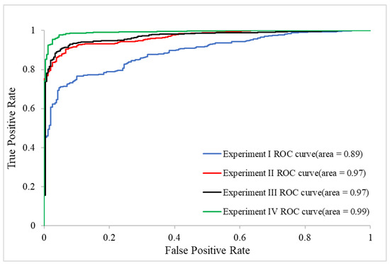
Figure 14.
The ROC curves and AUC of the RF classification models corresponding to the four experimental groups.
5.1.4. Optimizing the Boundary
Considering the spatial connectivity and integrity of urban and rural residential land, this study proposes a methodological process that first performs morphological closing-operation computing to connect fragmented patches filled with internal small-area natural elements and later screens and fills with large-area natural elements through pixel statistical analysis.
The size of the structural element window for the erosion and dilatation operators significantly impacts the extraction results of the boundaries [22,63]. To select a suitable window to optimize the effect of boundary extraction, this study set up nine different sizes of structural elements and found that a structural element of 13 × 13 can ensure the spatial connectivity of the URS and depict the detailed information of the boundary, which was highly consistent with the actual situation. Large-scale water bodies or green areas in a city cannot be processed by morphological closing operations and must be further recognized and filled. Since the area of natural elements in the city is much smaller than that of URSs, they can be extracted by detecting the ‘set of connected pixels with the same attribute value’ and setting the area threshold. It is worth noting that background objects also surround rural settlements, and the method extracts small rural settlement areas similarly. Natural elements and small rural settlements were extracted, and the final boundaries were obtained by uniformly changing the attribute values and overlaying them with the original image.
5.1.5. Potential Limitations
The method proposed in this study does not completely solve the problem of spectral confusion. In the Qinghai-Tibet Plateau region, there are numerous bare lands, sediments, and other land-cover types with spectral characteristics similar to those of urban and rural settlements, which may lead to errors in the extraction results. Additionally, the high heterogeneity of urban landscapes results in widespread mixed pixels, further reducing the classification accuracy.
5.2. Comparison with Existing Boundary Datasets
The URSB extracted in this study was compared with the GUB, CPUA, GHS-SMOD, and DUBC and displayed with high-resolution Google Earth imagery overlaid as the base map. The analysis revealed significant differences in the boundaries given by different researchers, owing to differences in the definition of land-use types, resolution of the data, and indicators of classification features. Figure 15 shows the differences between the three scales of area (entire administrative, urban, and village areas). The CPUA and DUBC ignored townships and rural areas and focused more on the boundaries of urban areas. The GUB includes cities and towns, excluding smaller towns and rural areas. The GHS-SMOD and this study contained both urban and rural area boundaries with high integrity. This suggests that most existing boundary products consider urban areas, ignoring urban fringe areas (suburbs) and villages. By contrast, this study considered the overall effect of boundaries on URSs. The boundaries extracted in this study and the GUB are closer to the actual URSB, whereas the CPUA, GHS-SMOD, and DUBC have different degrees of overestimation or underestimation of the extent of the city. Specifically, the boundaries extracted in this study and the GUB were irregularly shaped urban boundaries that were highly compatible with the actual situation, accurately separating the URS from background objects. The boundaries between GHS-SMOD and DUBC showed obvious regular zigzag shapes, which are usually caused by the low spatial resolution of the data used [9]. Although the CPUA used a higher-resolution image (2 m), the boundary details and accuracy were not as good as those extracted in this study and the GUB, probably because the multimodal land-use segmentation method was less effective in high-heterogeneity plateau cities. This further proves the importance of constructing feature indicators based on multi-source datasets.
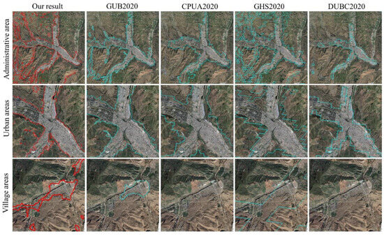
Figure 15.
Comparison of URSB in Xining, 2020. The red boundary is the result extracted from this paper, and the blue boundary is other datasets.
To further explore the accuracy and reliability of the boundary extraction in this study, two typical areas were selected for comparison with the GUB boundary (Figure 16). The integrity of the GUB boundary was low in the urban edge area, with the apparent omission of high-density impervious surfaces (Figure 16b). Regarding boundary details, the GUB mistakenly identified the mountains at the city’s edge as urban areas (Figure 16c), which is inconsistent with reality. This is due to the different indicators that generated the boundary of this study and the GUB boundary. The GUB boundary was obtained by secondary processing of the global artificial impervious area (GAIA) [64], whereas the GAIA classified non-arid areas [65] by considering only spectral feature metrics (NDVI, MNDWI, shortwave infrared bands, etc.). The extraction of the boundary in this study integrated spectral–topographic–SAR polarization features. Consequently, the boundaries extracted in this study have higher integrity, smoother and more continuous boundary contours, finer representations of boundary details, and stronger spatial consistency with the actual range.
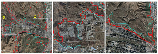
Figure 16.
Comparison of the details of this study boundary and the GUB boundary. (a) is the overlay display of the boundary of Xining in 2020; (b) is the zoomed-in view of the typical region A; (c) is the zoomed-in view of the typical region B; the red boundary is the result extracted from this paper, and the blue boundary is the GUB dataset.
6. Conclusions
In the context of rapid urban expansion, accurately monitoring the spatiotemporal patterns of urban and rural settlements is necessary to reveal the impacts of human activities on the ecological environment and for the sustainable development of cities. In this study, using Landsat 8, NASA DEM, and Sentinel-1 SAR as remote-sensing data sources, we developed an optimal random forest classification model for URSs based on spectral–topographic–radar polarization features. An optimal URSB extraction technique was established based on morphological and pixel-level statistical analyses. Using the Google Earth Engine (GEE) platform, the optimal random forest classification model for URSs and the URSB, the URSB of Xining in 2020 was extracted at a spatial resolution of 30 m, and the overall accuracy and Kappa coefficient were 96.21% and 0.92, respectively. The results demonstrate that spectral–topographic–SAR polarization feature synergy can achieve optimal mapping of URSs. They verified the effectiveness of the Blue Roof Index (BRI) proposed in this study in enhancing the information on high-reflectivity buildings. The results also showed that clear and definite vector boundaries could be obtained using the closing-operation method of morphology and neighborhood pixel statistics. Compared with the four existing urban boundary products (GUB2020, CPUA2020, GHS-SMOD2020, and DUBC2020), the boundaries extracted in this study are characterized by high spatial completeness and richer information in terms of details of urban fringe areas.
The method proposed in this study achieved excellent results in high-altitude plateau areas with complex terrains while demonstrating the potential application of URSB extraction in plain cities and coastal cities. This method should be tested for additional URS applications in the future. Future work involving monitoring at the subpixel scale should be conducted to address the common issue of mixed pixels.
Author Contributions
Conceptualization, G.Z.; methodology, X.L. (Xiaopeng Li); validation, X.L. (Xiaopeng Li), G.Z., L.Z., X.L. (Xiaoyang Li) and X.L. (Xiaomin Lv); formal analysis, G.Z. and L.Z.; data curation, X.L. (Xiaomin Lv); writing—original draft preparation, X.L. (Xiaopeng Li); writing—review and editing, G.Z.; funding acquisition, G.Z.; supervision, X.H. and Z.T. All authors have read and agreed to the published version of the manuscript.
Funding
This research was funded by the Second Tibetan Plateau Comprehensive Research Project (2019QZKK0106), the National Natural Science Foundation of China (42130514), and Fundamental Research Funds of the Chinese Academy of Meteorological Sciences (2020Z004, 2022Y015).
Data Availability Statement
Data are contained within the article.
Acknowledgments
We thank the Google Earth Engine Science team for the freely available cloud computing platform and the USGS for the Landsat imagery and NASA DEM.
Conflicts of Interest
The authors declare no conflicts of interest.
References
- Zhang, J.; Feng, Z.; Jiang, L. Progress on studies of land use/land cover classification systems. Resour. Sci. 2011, 33, 1195–1203. (In Chinese) [Google Scholar]
- Huang, X.; Yang, J.; Wang, W.; Liu, Z. Mapping 10 m global impervious surface area (GISA-10 m) using multi-source geospatial data. Earth Syst. Sci. Data 2022, 14, 3649–3672. [Google Scholar] [CrossRef]
- Folke, C.; Jansson, A.; Larsson, J.; Costanza, R. Ecosystem appropriation by cities. Ambio 1997, 26, 167–172. [Google Scholar]
- Sun, Y.; Zhao, S.; Qu, W. Quantifying spatiotemporal patterns of urban expansion in three capital cities in Northeast China over the past three decades using satellite data sets. Environ. Earth Sci. 2015, 73, 7221–7235. [Google Scholar] [CrossRef]
- McGrane, S.J. Impacts of urbanisation on hydrological and water quality dynamics, and urban water management: A review. Hydrol. Sci. J. 2016, 61, 2295–2311. [Google Scholar] [CrossRef]
- Masson, V.; Lemonsu, A.; Hidalgo, J.; Voogt, J. Urban climates and climate change. Annu. Rev. Environ. Resour. 2020, 45, 411–444. [Google Scholar] [CrossRef]
- Güneralp, B.; Seto, K. Futures of global urban expansion: Uncertainties and implications for biodiversity conservation. Environ. Res. Lett. 2013, 8, 014025. [Google Scholar] [CrossRef]
- Wei, Y.D.; Ye, X. Urbanization, urban land expansion and environmental change in China. Stoch. Environ. Res. Risk Assess. 2014, 28, 757–765. [Google Scholar] [CrossRef]
- Li, X.; Gong, P.; Zhou, Y.; Wang, J.; Bai, Y.; Chen, B.; Hu, T.; Xiao, Y.; Xu, B.; Yang, J. Mapping global urban boundaries from the global artificial impervious area (GAIA) data. Environ. Res. Lett. 2020, 15, 094044. [Google Scholar] [CrossRef]
- Dai, X.; Jin, J.; Chen, Q.; Fang, X. On Physical Urban Boundaries, Urban Sprawl, and Compactness Measurement: A Case Study of the Wen-Tai Region, China. Land 2022, 11, 1637. [Google Scholar] [CrossRef]
- Hu, S.; Tong, L.; Frazier, A.E.; Liu, Y. Urban boundary extraction and sprawl analysis using Landsat images: A case study in Wuhan, China. Habitat Int. 2015, 47, 183–195. [Google Scholar] [CrossRef]
- Zhou, Y.; Li, X.; Asrar, G.R.; Smith, S.J.; Imhoff, M. A global record of annual urban dynamics (1992–2013) from nighttime lights. Remote Sens. Environ. 2018, 219, 206–220. [Google Scholar] [CrossRef]
- Zha, Y.; Gao, J.; Ni, S. Use of normalized difference built-up index in automatically mapping urban areas from TM imagery. Int. J. Remote Sens. 2003, 24, 583–594. [Google Scholar] [CrossRef]
- Xu, H. A new index for delineating built-up land features in satellite imagery. Int. J. Remote Sens. 2008, 29, 4269–4276. [Google Scholar] [CrossRef]
- Peng, J.; Zhao, S.; Liu, Y.; Tian, L. Identifying the urban-rural fringe using wavelet transform and kernel density estimation: A case study in Beijing City, China. Environ. Model. Softw. 2016, 83, 286–302. [Google Scholar] [CrossRef]
- Tao, Y.; Liu, W.; Chen, J.; Gao, J.; Li, R.; Ren, J.; Zhu, X. A Self-Supervised Learning Approach for Extracting China Physical Urban Boundaries Based on Multi-Source Data. Remote Sens. 2023, 15, 3189. [Google Scholar] [CrossRef]
- Taubenböck, H.; Weigand, M.; Esch, T.; Staab, J.; Wurm, M.; Mast, J.; Dech, S. A new ranking of the world’s largest cities—Do administrative units obscure morphological realities? Remote Sens. Environ. 2019, 232, 111353. [Google Scholar] [CrossRef]
- Xu, Z.; Jiao, L.; Lan, T.; Zhou, Z.; Cui, H.; Li, C.; Xu, G.; Liu, Y. Mapping hierarchical urban boundaries for global urban settlements. Int. J. Appl. Earth Obs. Geoinf. 2021, 103, 102480. [Google Scholar] [CrossRef]
- Liu, S.; Shi, K.; Wu, Y. Identifying and evaluating suburbs in China from 2012 to 2020 based on SNPP—VIIRS nighttime light remotely sensed data. Int. J. Appl. Earth Obs. Geoinf. 2022, 114, 103041. [Google Scholar] [CrossRef]
- Zhang, X.; Liu, L.; Wu, C.; Chen, X.; Gao, Y.; Xie, S.; Zhang, B. Development of a global 30 m impervious surface map using multisource and multitemporal remote sensing datasets with the Google Earth Engine platform. Earth Syst. Sci. Data 2020, 12, 1625–1648. [Google Scholar] [CrossRef]
- Zhao, M.; Cheng, C.; Zhou, Y.; Li, X.; Shen, S.; Song, C. A global dataset of annual urban extents (1992–2020) from harmonized nighttime lights. Earth Syst. Sci. Data 2022, 14, 517–534. [Google Scholar] [CrossRef]
- Wang, Z.; Wang, H.; Qin, F.; Han, Z.; Miao, C. Mapping an Urban Boundary Based on Multi-Temporal Sentinel-2 and POI Data: A Case Study of Zhengzhou City. Remote Sens. 2020, 12, 4103. [Google Scholar] [CrossRef]
- He, C.; Liu, Z.; Tian, J.; Ma, Q. Urban expansion dynamics and natural habitat loss in China: A multiscale landscape perspective. Glob. Chang. Biol. 2014, 20, 2886–2902. [Google Scholar] [CrossRef] [PubMed]
- Florczyk, A.J.; Melchiorri, M.; Corbane, C.; Schiavina, M.; Maffenini, M.; Pesaresi, M.; Politis, P.; Sabo, S.; Freire, S.; Ehrlich, D.; et al. Description of the GHS Urban Centre Database 2015, Public Release 2019, Version 1.0; Technical Report; Publications Office of the European Union: Luxembourg, 2019. [Google Scholar] [CrossRef]
- Xining. Available online: https://en.wikipedia.org/wiki/Xining (accessed on 5 October 2023).
- Schubert, A.; Small, D.; Miranda, N.; Geudtner, D.; Meier, E. Sentinel-1A product geolocation accuracy: Commissioning phase results. Remote Sens. 2015, 7, 9431–9449. [Google Scholar] [CrossRef]
- Buckley, S. NASADEM Merged DEM Global 1 Arc Second V001 [Data Set]. In NASA EOSDIS Land Processes DAAC; USGS: Reston, VA, USA, 2020. [Google Scholar] [CrossRef]
- Zhang, X.; Du, S.; Zhou, Y.; Xu, Y. Extracting physical urban areas of 81 major Chinese cities from high-resolution land uses. Cities 2022, 131, 104061. [Google Scholar] [CrossRef]
- Schiavina, M.; Melchiorri, M.; Pesaresi, M. GHS-SMOD R2023A—GHS Settlement Layers, Application of the Degree of Urbanisation Methodology (Stage I) to GHS-POP R2023A and GHS-BUILT-S R2023A, Multitemporal (1975–2030); European Commission, Joint Research Centre (JRC): Petten, The Netherlands, 2023. [Google Scholar] [CrossRef]
- Bauer, M.E.; Heinert, N.J.; Doyle, J.K.; Yuan, F. Impervious surface mapping and change monitoring using Landsat remote sensing. In Proceedings of the ASPRS 2004 Annual Conference on Mountains of Data Peak Decisions, Denver, CO, USA, 23–28 May 2004. [Google Scholar]
- Huang, R.; Xu, H. A study on the relationship between land cover/use and urban heat environment using Landsat ETM+ satellite imagery: A case study of Fuzhou. Remote Sens. Inf. 2005, 2005, 36–39. (In Chinese) [Google Scholar]
- Xu, H. Analysis of impervious surface and its impact on urban heat environment using the normalized difference impervious surface index (NDISI). Photogramm. Eng. Remote Sens. 2010, 76, 557–565. [Google Scholar] [CrossRef]
- Mu, Y.; Xie, Y.; Zhang, L.; Chen, Y. An enhanced normalized difference impervious surface index. Sci. Surv. Mapp. 2018, 43, 83–87. [Google Scholar] [CrossRef]
- Xu, H. A study on information extraction of water body with the modified normalized difference water index (MNDWI). J. Remote Sens. 2005, 9, 595. [Google Scholar]
- Tucker, C.J. Red and photographic infrared linear combinations for monitoring vegetation. Remote Sens. Environ. 1979, 8, 127–150. [Google Scholar] [CrossRef]
- Huete, A.; Didan, K.; Miura, T.; Rodriguez, E.P.; Gao, X.; Ferreira, L.G. Overview of the radiometric and biophysical performance of the MODIS vegetation indices. Remote Sens. Environ. 2002, 83, 195–213. [Google Scholar] [CrossRef]
- Jordan, C.F. Derivation of leaf-area index from quality of light on the forest floor. Ecology 1969, 50, 663–666. [Google Scholar] [CrossRef]
- Richardson, A.J.; Wiegand, C. Distinguishing vegetation from soil background information. Photogramm. Eng. Remote Sens. 1977, 43, 1541–1552. [Google Scholar]
- Ji, H.; Li, X.; Wei, X.; Liu, W.; Zhang, L.; Wang, L. Mapping 10-m resolution rural settlements using multi-source remote sensing datasets with the Google Earth Engine platform. Remote Sens. 2020, 12, 2832. [Google Scholar] [CrossRef]
- Ren, H.; Liu, Y.; Chang, X.; Yang, J.; Xiao, X.; Huang, X. Mapping High-Resolution Global Impervious Surface Area: Status and Trends. IEEE J. Sel. Top. Appl. Earth Obs. Remote Sens. 2022, 15, 7288–7307. [Google Scholar] [CrossRef]
- Breiman, L. Random forests. Mach. Learn. 2001, 45, 5–32. [Google Scholar] [CrossRef]
- Tang, P.; Du, P.; Lin, C.; Guo, S.; Qie, L. A novel sample selection method for impervious surface area mapping using JL1-3B nighttime light and Sentinel-2 imagery. IEEE J. Sel. Top. Appl. Earth Obs. Remote Sens. 2020, 13, 3931–3941. [Google Scholar] [CrossRef]
- dos Anjos, C.S.; Lacerda, M.G.; do Livramento Andrade, L.; Salles, R.N. Classification of urban environments using feature extraction and random forest. In Proceedings of the 2017 IEEE International Geoscience and Remote Sensing Symposium (IGARSS), Fort Worth, TX, USA, 23–28 July 2017; pp. 1205–1208. [Google Scholar] [CrossRef]
- Shih, H.-C.; Stow, D.A.; Chang, K.-C.; Roberts, D.A.; Goulias, K.G. From land cover to land use: Applying random forest classifier to Landsat imagery for urban land-use change mapping. Geocarto Int. 2022, 37, 5523–5546. [Google Scholar] [CrossRef]
- Gislason, P.O.; Benediktsson, J.A.; Sveinsson, J.R. Random forests for land cover classification. Pattern Recognit. Lett. 2006, 27, 294–300. [Google Scholar] [CrossRef]
- Bach, F. Breaking the curse of dimensionality with convex neural networks. J. Mach. Learn. Res. 2017, 18, 629–681. [Google Scholar]
- Zourarakis, D.P. Remote Sensing Handbook—Volume I: Remotely Sensed Data Characterization, Classification, and Accuracies. Photogramm. Eng. Remote Sens. 2018, 84, 481. [Google Scholar] [CrossRef]
- Benediktsson, J.A.; Pesaresi, M.; Amason, K. Classification and feature extraction for remote sensing images from urban areas based on morphological transformations. IEEE Trans. Geosci. Remote Sens. 2003, 41, 1940–1949. [Google Scholar] [CrossRef]
- Liang, X.; Liu, X.; Li, X.; Chen, Y.; Tian, H.; Yao, Y. Delineating multi-scenario urban growth boundaries with a CA-based FLUS model and morphological method. Landsc. Urban Plan. 2018, 177, 47–63. [Google Scholar] [CrossRef]
- Narayanan, A. Fast binary dilation/erosion algorithm using kernel subdivision. In Proceedings of the Asian Conference on Computer Vision, ACCV 2006, Hyderabad, India, 13–16 January 2006; Springer: Berlin/Heidelberg, Germany, 2006; Volume 3852, pp. 335–342. [Google Scholar]
- Canny, J. A computational approach to edge detection. IEEE Trans. Pattern Anal. Mach. Intell. 1986, 6, 679–698. [Google Scholar] [CrossRef]
- Li, X.; Chen, G.; Zhang, Y.; Yu, L.; Du, Z.; Hu, G.; Liu, X. The impacts of spatial resolutions on global urban-related change analyses and modeling. iScience 2022, 25, 105660. [Google Scholar] [CrossRef]
- White, J.C.; Wulder, M.; Hobart, G.; Luther, J.; Hermosilla, T.; Griffiths, P.; Coops, N.; Hall, R.; Hostert, P.; Dyk, A. Pixel-based image compositing for large-area dense time series applications and science. Can. J. Remote Sens. 2014, 40, 192–212. [Google Scholar] [CrossRef]
- Zhang, Z.; Wei, M.; Pu, D.; He, G.; Wang, G.; Long, T. Assessment of annual composite images obtained by Google Earth engine for urban areas mapping using random forest. Remote Sens. 2021, 13, 748. [Google Scholar] [CrossRef]
- Pu, D.C.; Sun, J.Y.; Ding, Q.; Zheng, Q.; Li, T.T.; Niu, X.F. Mapping urban areas using dense time series of landsat images and google earth engine. Int. Arch. Photogramm. Remote Sens. Spat. Inf. Sci.—ISPRS Arch. 2020, 42, 403–409. [Google Scholar] [CrossRef]
- Wang, Y.; Li, M. Urban impervious surface automatic threshold detection model derived from multitemporal Landsat images. IEEE Trans. Geosci. Remote Sens. 2021, 60, 4503321. [Google Scholar] [CrossRef]
- Zhang, Y.; Zhang, H.; Lin, H. Improving the impervious surface estimation with combined use of optical and SAR remote sensing images. Remote Sens. Environ. 2014, 141, 155–167. [Google Scholar] [CrossRef]
- Clarke, K.C.; Hoppen, S.; Gaydos, L. A self-modifying cellular automaton model of historical urbanization in the San Francisco Bay area. Environ. Plan. B 1997, 24, 247–261. [Google Scholar] [CrossRef]
- Liu, X.; Hu, G.; Chen, Y.; Li, X.; Xu, X.; Li, S.; Pei, F.; Wang, S. High-resolution multi-temporal mapping of global urban land using Landsat images based on the Google Earth Engine Platform. Remote Sens. Environ. 2018, 209, 227–239. [Google Scholar] [CrossRef]
- Li, X.; Gong, P. An “exclusion-inclusion” framework for extracting human settlements in rapidly developing regions of China from Landsat images. Remote Sens. Environ. 2016, 186, 286–296. [Google Scholar] [CrossRef]
- Behnamian, A.; Millard, K.; Banks, S.N.; White, L.; Richardson, M.; Pasher, J. A systematic approach for variable selection with random forests: Achieving stable variable importance values. IEEE Geosci. Remote Sens. Lett. 2017, 14, 1988–1992. [Google Scholar] [CrossRef]
- Hand, D.J.; Anagnostopoulos, C. When is the area under the receiver operating characteristic curve an appropriate measure of classifier performance? Pattern Recogn. Lett. 2013, 34, 492–495. [Google Scholar] [CrossRef]
- Huang, K.; Dai, W.; Huang, W.; Ou, H. Study on the delimitation of urban growth boundary based on FLUS model and kinetic energy theorem. J. Geo-Inf. Sci. 2020, 22, 557–567. [Google Scholar] [CrossRef]
- Gong, P.; Li, X.; Wang, J.; Bai, Y.; Chen, B.; Hu, T.; Liu, X.; Xu, B.; Yang, J.; Zhang, W. Annual maps of global artificial impervious area (GAIA) between 1985 and 2018. Remote Sens. Environ. 2020, 236, 111510. [Google Scholar] [CrossRef]
- Olson, D.M.; Dinerstein, E.; Wikramanayake, E.D.; Burgess, N.D.; Powell, G.V.; Underwood, E.C.; D’amico, J.A.; Itoua, I.; Strand, H.E.; Morrison, J.C. Terrestrial Ecoregions of the World: A New Map of Life on Earth: A new global map of terrestrial ecoregions provides an innovative tool for conserving biodiversity. BioScience 2001, 51, 933–938. [Google Scholar] [CrossRef]
Disclaimer/Publisher’s Note: The statements, opinions and data contained in all publications are solely those of the individual author(s) and contributor(s) and not of MDPI and/or the editor(s). MDPI and/or the editor(s) disclaim responsibility for any injury to people or property resulting from any ideas, methods, instructions or products referred to in the content. |
© 2024 by the authors. Licensee MDPI, Basel, Switzerland. This article is an open access article distributed under the terms and conditions of the Creative Commons Attribution (CC BY) license (https://creativecommons.org/licenses/by/4.0/).