Spectral-Spatial Domain Attention Network for Hyperspectral Image Few-Shot Classification

Abstract

Recently, many deep learning-based methods have been successfully applied to hyperspectral image (HSI) classification. Nevertheless, training a satisfactory network usually needs enough labeled samples. This is unfeasible in practical applications since the labeling of samples is time-consuming and expensive. The target domain samples that need to be classified are usually limited in HSIs. To mitigate this issue, a novel spectral-spatial domain attention network (SSDA) is proposed for HSI few-shot classification, which can transfer the learned classification knowledge from source domain contained enough labeled samples to target domain. The SSDA includes a spectral-spatial module, a domain attention module, and a multiple loss module. The spectral-spatial module can learn discriminative and domain invariance spectral-spatial features. The domain attention module can further enhance useful spectral-spatial features and avoid the interference of useless features. The multiple loss module, including few-shot loss, coral loss, and mmd loss, can solve the domain adaptation issue. Extensive experimental results demonstrate that on the Salinas, the University of Pavia (UP), the Indian Pines (IP), and the Huoshaoyun datasets, the proposed SSDA obtains higher classification accuracies than state-of-the art methods in the HSI few-shot classification.

1. Introduction

Hyperspectral images contain hundreds of bands, with rich spectral and spatial information [1]. They have been explored in many areas, such as HSI classification [2], geological survey [3], biomedicine [4]. In particular, the HSI classification task is the basis of HSI analysis. It allocates a label to each pixel. However, the acquisition and learning of HSI features have always been the focus of and difficult in HSI classification research. How sufficiently and effectively features are extracted directly affects the classification results.

In the early stages of research, most of classification methods are mainly handcrafted feature extraction [5] and conventional classifiers. The widely used handcraft feature extraction methods contain principal component analysis (PCA) [6], linear discriminant analysis (LDA) [7], and simple linear iterative cluster (SLIC) [8]. Feng Xue et al. proposed an improved functional principal component analysis method, which can extract more effective functional features by making full use of the label information of training samples [6]. Qiuling Hou et al. proposed a novel supervised dimensionality reduction method termed linear discriminant analysis based on kernel-based possibilistic c-means, which use a KPCM algorithm to generate different weights for different samples [7]. Munmun Baisantry et al. proposed a band selection technique based on the FDA and functional PCA fusion method. This method can select shape-preserving, discriminative bands that can highlight the important characteristics, variations as well as patterns of the hyperspectral data [9]. Conventional classifiers mainly contain support vector machine (SVM) [10], k-nearest neighbor (KNN) [11], logistic regression [12], and so on. Amos Bortiew et al. proposed an active learning method for HSI classification using kernel sparse representation classifiers (KSRC). KSRC has proven to be a robust classifier and has successfully been applied to HSI classification [13]. Nevertheless, the handcrafted features extracted by these methods usually have weak representative and discriminative feature characteristics, which result in unsatisfactory classification performance.

Recently, learning-based methods have been applied to classify HSIs and have achieved great success due to their greater representation ability [2,14,15,16,17,18,19,20,21,22,23,24,25,26,27,28]. Yushi Chen et al. [2] designed a stacked autoencoder to learn spectral information and spatial information. Then, they proposed a deep learning framework combined PCA and logistic regression to fuse two kinds of features. The classifier of the deep learning method unsurprisingly achieved higher accuracy. Yushi Chen et al. [29] further designed a new deep framework that combined spectral spatial feature extraction and classifier to improve classification accuracy. Wei Hu et al. [20] presented a simple CNN architecture that contained multiple convolutional layers for classification. Jiaojiao Li et al. [21] proposed a full CNN to learn HSI features. Furthermore, a deconvolution network was proposed to enhance HSI features. Qichao Liu et al. [18] proposed a novel guided feature extraction unit, which can enhance the cross-classes region features and suppress the irregular features. Ghaderizadeh Saeed et al. [17] proposed a mixed 3D–2D CNN, which could learn the useful spectral-spatial features. Weiwei Song et al. proposed a novel hashing-based deep metric learning method for hyperspectral images and light detection and ranging data classification. They also elaborately designed a loss function to simultaneously consider the label-based semantic loss and hashing-based metric loss [23]. Tan Guo et al. designed a dual-view spectral and global spatial feature fusion network to extract the spatial-spectral features, which included a spatial subnetwork and a spectral subnetwork [22]. Hao Zhou et al. proposed a novel multiple feature fusion model, which included two subnetworks of multiscale fully CNN and multihop GCN to extract the multilevel information from HSIs [24]. Yule Duan et al. proposed a structure-preserved hyper GCN, which integrated local regular convolution and irregular hypergraph convolution to learn the structured semantic feature of HSIs [25]. M.E.Paoletti et al. presented a novel classification method combined the ghost-module architecture with a CNN-based HSI classifier to reduce the computational cost, which can achieve a satisfactory classification performance [26]. Swalpa Kumar Roy et al. proposed a new end-to-end morphological deep learning framework to model nonlinear information during the training process. The method included spectral and spatial morphological blocks to extract relevant features from the HSI data [27]. Kazem Safari et al. proposed a deep learning strategy that combined different convolutional neural networks to efficiently extract joint spatial-spectral features over multiple scales [28]. Although these learning-based methods have more advantages than conventional methods in HSI classification, they inevitably require extensive labeled samples to train a suitable network for classification. Nevertheless, it is usually difficult to obtain labeled samples to train a good performing neural network, because the collection of labeled samples requires a lot of time and financial resources.

To mitigate this issue, many scholars have introduced unsupervised methods to assist in HSI classification [30,31,32]. Shaohui Mei et al. [30] designed an unsupervised feature learning method with 3D convolutional autoencoder (3D-CAE), which could effectively learn spatial-spectral structure features. Lichao Mou et al. [31] proposed an unsupervised network architecture, which introduced an encoder-decoder architecture to extract unsupervised spectral-spatial features to assist classification.

Meanwhile, some researchers have also presented semi-supervised approaches [33,34,35]. Kun Tan et al. [33] argued that spatial neighborhood information of samples is very useful in the semi-supervised HSI classification. Therefore, they used spatial neighborhood information to enhance the classifier to improve the classification performance. Yue Wu et al. [34] designed a semi-supervised approach to fully extract unlabeled samples information. Further, they used a self-training method to gradually increase the sample points confidence, which could enhance the semi-supervised HSI classification ability. Fuding Xie et al. [35] developed a multinomial logistic regression module and a local mean-based pseudo nearest neighbor module to learn labeled samples information. Then, a novel four steps strategy was proposed to conduct semi-supervised classification. The above methods indeed achieved good classification performance in the case of limited samples. But they mainly learned the limited labeled features or further explored the features of unlabeled samples to train the model. It meant that the labeled samples were exactly identical to the unlabeled samples, which resulted in a network performance always limited by the number of labeled samples from the target domain data to be classified (namely, the target domain). Meanwhile, they also hardly utilized enough labeled samples in other HSIs [36] (namely, the source domain). In practice, the distribution of the source domain and the target domain may be different, which makes it difficult to improve the accuracy of HSI few-shot classification.

To further resolve this issue, meta-learning methods have been proposed to learn classification abilities from HSIs [37,38]. In particular, meta-learning does not require strict class consistency and the same distribution between source domain and target domain. Few-shot learning (FSL) is an important implementation method of meta-learning [39,40,41], which can transfer the extracted classification knowledge from source domain to target domain. In recent years, a growing number of FSL methods have been proposed for HSI classification [42,43,44,45]. Bing Liu et al. [42] proposed a deep FSL method to solve the small sample size problem of HSI classification via learning the metric space from the training set. Kuiliang Gao et al. [43] designed a novel classification method based on relational network and trained it using the idea of meta-learning. Xuejian Liang et al. [44] proposed an attention multisource fusion method for HSI few-shot classification, which could extract features from fused homogeneous and heterogeneous data. Xibing Zuo et al. [45] proposed an edge-labeling graph neural network, which could explicitly quantify the intraclass and interclass features between different pixels.

Although these FSL methods have achieved good classification accuracy with the limited labeled samples, the feature extraction ability of the source and target domain data is still the main factor affecting classification accuracy and thus needs to be improved. Meanwhile, it is necessary to further enhance useful spectral-spatial features and repress useless features to improve the classification accuracy. To this end, a novel spectral-spatial domain attention network (SSDA) is developed in this article. It is composed of a spectral-spatial module, a domain attention module and a multiple loss module. The spectral-spatial module is designed to extract discriminative and domain invariance spectral-spatial features via a spectral branch and a multiscale spatial branch. The domain attention module is proposed to enhance the contributions of useful spectral-spatial features. The multiple loss module contains few-shot loss, coral loss, and mmd loss, which can jointly solve the domain adaptation issue. In particular, the few-shot loss is utilized to minimize the cross entropy between the predicted probability and the ground truth. The coral loss is utilized to minimize the difference in learned feature covariances between source domain and target domain. The mmd loss is utilized to reduce the distribution differences between source domain and target domain. Extensive experimental results demonstrate that on the Salinas, University of Pavia (UP), Indian Pines (IP), and Huoshaoyun datasets, the proposed method achieves higher classification accuracy than state-of-the-art methods with few-shot samples. This article mainly contains three contributions.

• To extract discriminative and domain invariance spectral-spatial features, a spectral-spatial module is developed via a spectral branch and a multiscale spatial branch. The residual deformable 3D block of the spectral branch can learn rich spectral features, which can well adapt to the spatial geometric transformations. The multiscale spatial branch can learn multiscale spatial features, which can learn strong complementary and related spatial information.
• Different spectral-spatial features make different contributions to classification. The domain attention module is designed via a spectral attention block and a spatial attention block to further enhance useful spectral-spatial features and suppress useless features.
• By combining the spectral-spatial module, the domain attention module, and the multiple loss module, a novel spectral-spatial domain attention (SSDA) method is proposed. It can transfer the classification knowledge from source domain to target domain to improve the HSI few-shot classification accuracy.

2. Related Work

In this part, we firstly review the definition of few-shot learning, then introduce some basic networks, such as the 3D convolution and the deformable convolution.

2.1. Few-Shot Learning

Few-shot learning is inspired by the rapid learning mechanism of the human brain. Humans are very adept at identifying new targets via a very few shot samples. For example, a child usually needs a few shot samples to recognize what a “tiger” is and what a “rabbit” is. Few-shot learning is one of the applications of meta-learning [46]. In detail, researchers hope that after learning many labeled samples (namely source domain), the learning model can transfer the learned ability of classification to new categories of few shot labeled samples (target domain). Specifically, during the training phase, C classes are randomly selected from the two domains, with K samples in each class (total $C\times K$ samples), and a meta-task are constructed as the input of the learning model’s support set. A batch of samples is extracted from the remaining samples as the query set. That is, the meta-task requires the learning model to learn how to distinguish the C classes from $C\times K$ samples, which is called the C-way K-shot problem.

2.2. The 3D Convolution and the Deformable Convolution

Traditional CNN usually processes two-dimensional images, and the convolution kernel used is also two-dimensional, but HSIs have an additional spectral dimension. The 3D-CNN uses three-dimensional convolution to directly learn the spectral and spatial information of HSIs [47] simultaneously. Therefore, the 3D-CNN is more suitable for HSI few-shot classification.

However, the traditional 3D convolution kernel is usually fixed in size, which makes it difficult to handle the spatial geometric transformations. To solve this problem, a 3D deformable convolution operation is designed via combining 3D convolution and deformable convolution [48].

The 3D convolution kernel G can be represented as:

$$G=(-1,-1,-1),(-1,-1,0),\cdots ,(1,1,0),(1,1,1)$$

(1)

Therefore, for each location $f_0$ on the output feature map y, we have:

$$y\left(f_0\right)=\sum _{g_n\in G}w\left(g_n\right)·x\left(f_0+g_n\right)$$

(2)

where x is the input of the feature, w is the weight matrix value of the convolution layer, and y is the output of the feature. $g_n$ enumerates the locations in the convolution kernel G. In 3D deformable convolution, the 3D convolution kernel G is augmented with offsets $\left\{\Delta g_n|n=1,\cdots ,N\right\}$, where $N=\left|G\right|$. The 3D deformable convolution can be represented as:

$$y\left(f_0\right)=\sum _{g_n\in G}w\left(g_n\right)·x\left(f_0+g_n+\Delta g_n\right)$$

(3)

3. Materials and Methods

In this section, the spectral-spatial domain attention network (SSDA) architecture will be introduced in detail, which includes a spectral-spatial module, a domain attention module, and a multiple loss module.

3.1. SSDA Framework

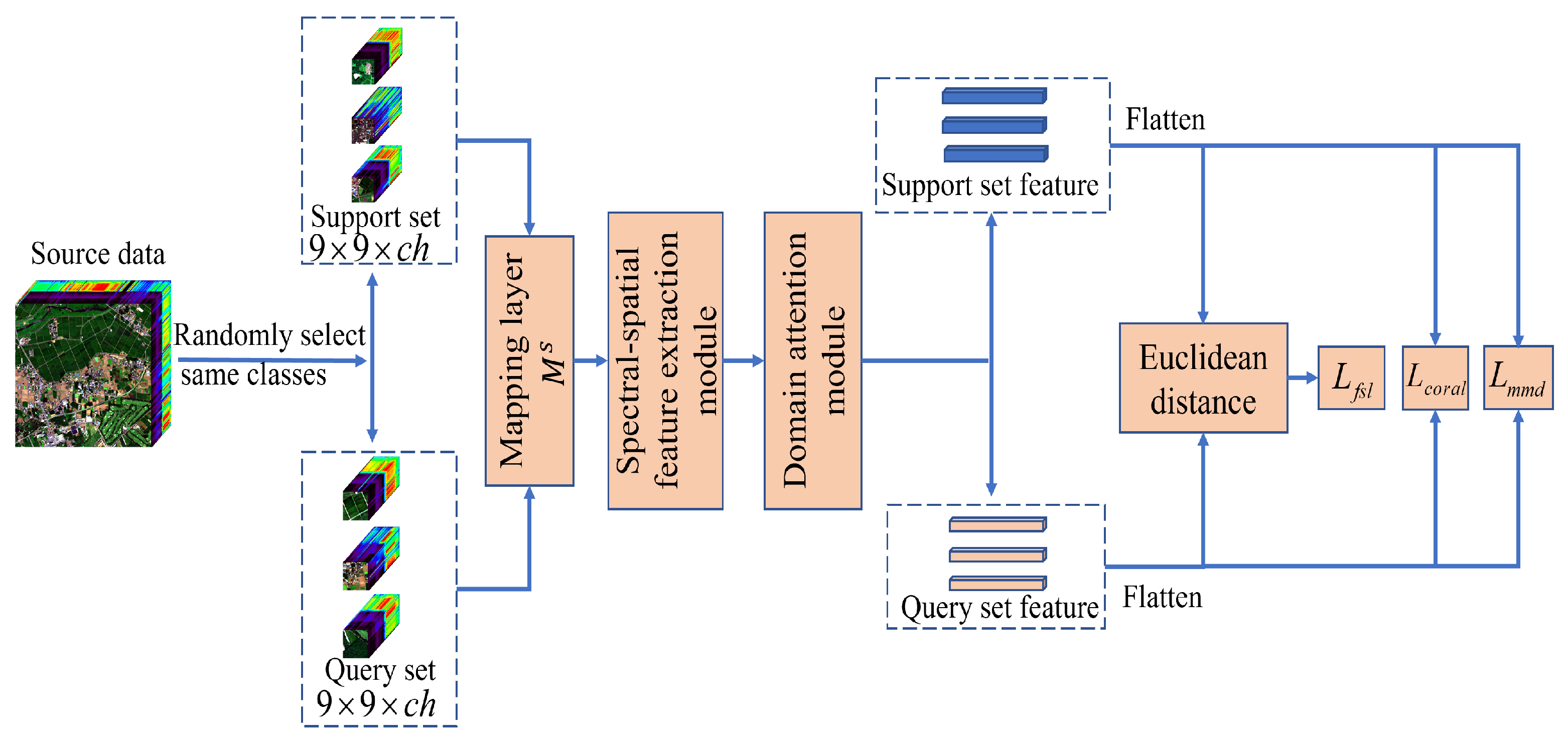
Figure 1 displays the training framework of the SSDA. In particular, the SSDA contains two types of FSL. One is the source domain FSL. The other is the FSL for few-shot labeled samples in the target domain data. Two types of FSL are executed alternately. For each kind of FSL, there are four steps. First, we designed two mapping layers ($M^s$ and $M^t$) to generate the same cube size from the source domain and target domain separately. Second, a spectral-spatial module was proposed to learn the discriminative and domain invariance spectral-spatial features via a spectral branch and a multiscale spatial branch. Third, a domain attention module was designed to learn the informative and discriminative spectral-spatial features, which can enhance useful features and avoid the interference of useless features. Finally, to solve domain adaptation issue, we performed the source domain FSL by calculating distances between th support set features and the query set features of each class. Similarly, we could also perform the target domain FSL. Therefore, we obtained the fsl loss ($L_{fsl}$), the coral loss ($L_{coral}$), and the mmd loss ($L_{mmd}$) on the source domain and the target domain separately.

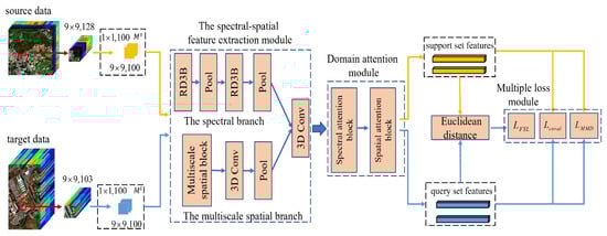
Figure 1. The proposed spectral-spatial domain attention network (SSDA) for HSI few-shot classification in the training phase.

Therefore, total loss function of source domain FSL can be repressed by

$$L_{total}^s=L_{fsl}^s+L_{coral}^s+L_{mmd}^s$$

(4)

Total loss of target domain FSL can be represented by

$$L_{total}^t=L_{fsl}^t+L_{coral}^t+L_{mmd}^t$$

(5)

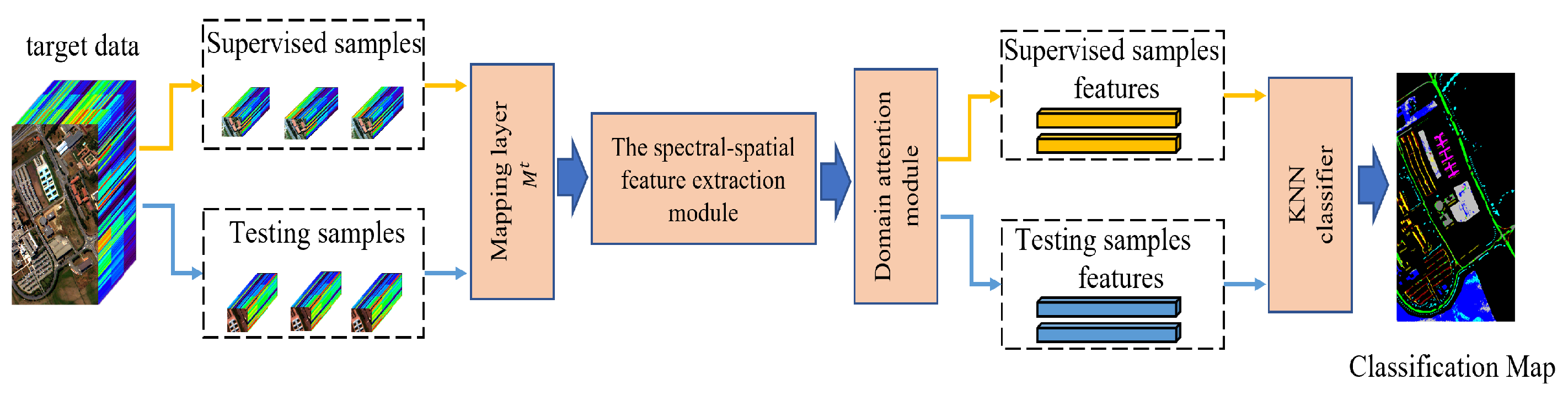
Moreover, Figure 2 shows the classification process of the testing phase. It also contains four steps. First, we used the target mapping layer ($M^t$) to reduce the number of bands of input samples. Second, the spectral-spatial module learned the supervised samples features and the testing samples features separately. Third, a domain attention module was utilized to enhance useful features. Finally, a KNN classifier was utilized to predict the testing samples.

Figure 2. The schematic diagram of the SSDA classification in the testing phase.

3.2. The Mapping Layer and the Spectral-Spatial Module

HSIs usually contain tens to hundreds of bands with redundant spectral information. It always leads to high computational complexity. Therefore, we needed to perform certain preprocessing on the HSIs, which maps the high-dimensional raw cube to low-dimensional feature cube. In this case, we sent the data cubes of the same spatial size ($9\times 9$) from the source and target domains to the mapping layer to generate the new source domain and target domain data cubes with the same spectral dimensions ($9\times 9\times 100$).

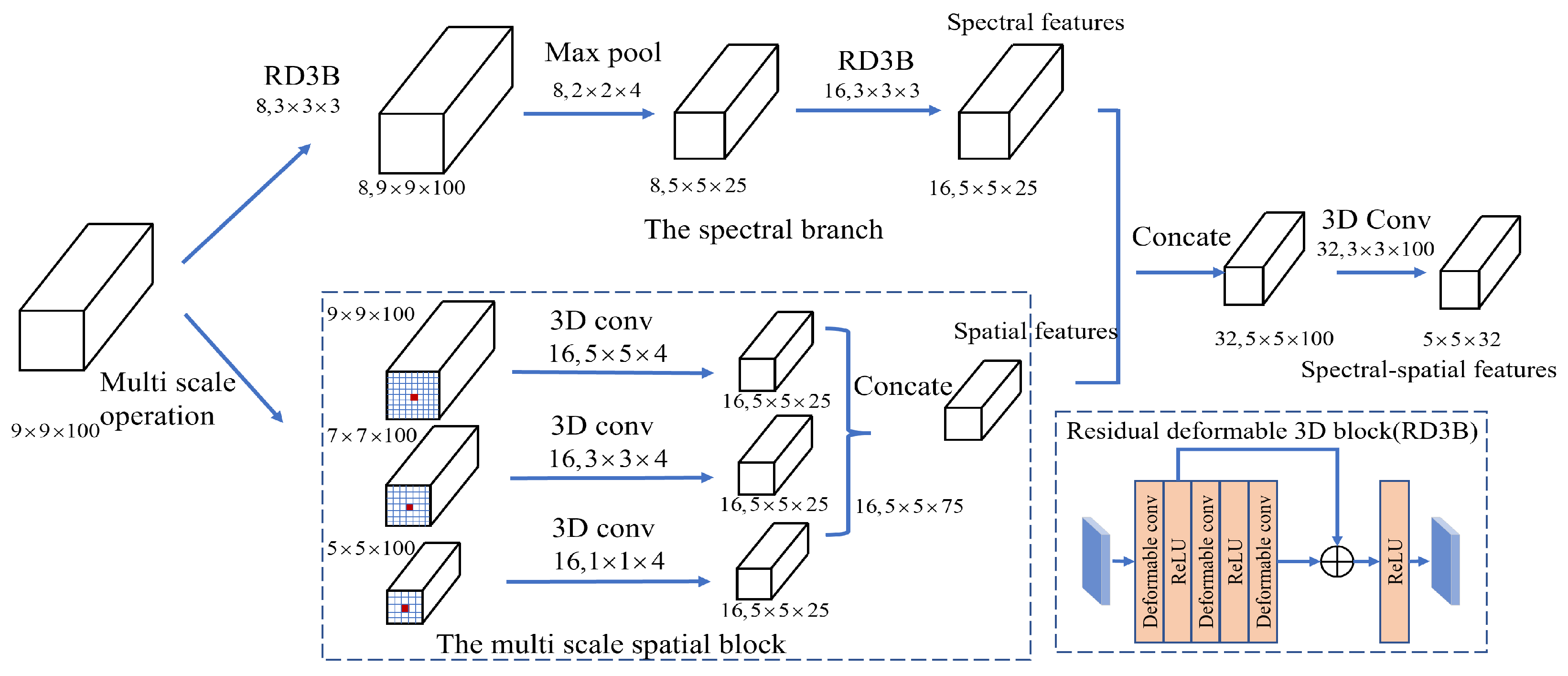
To further learn the rich spectral-spatial features from source domain and target domain data, we designed a novel spectral-spatial module (Figure 3) that contained a spectral branch and a multiscale spatial branch. The spectral branch contained two residual deformable 3D blocks (RD3B) and a max pooling layer, which could extract rich spectral features that could well adapt to the spatial geometric transformations. In particular, the RD3B contained three 3D deformable convolution layers and a shortcut. The multiscale spatial branch contained a multiscale spatial block and a concatenate operation, which could learn multiscale spatial features. In particular, the multiscale spatial block contained three different spatial scale cubes ($9\times 9\times 100$, $7\times 7\times 100$, $5\times 5\times 100$). Three different 3D convolution layers ($16,5\times 5\times 4$, $16,3\times 3\times 4$, $16,1\times 1\times 4$) could be utilized to generate the same size spatial scale features ($16,5\times 5\times 25$). Different spatial scale features have strong complementary and related information. After the spectral-spatial module, the feature dimension output by the feature extractor is $5\times 5\times 32$.

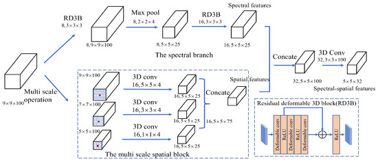
Figure 3. The spectral-spatial module contains a spectral branch and a multiscale spatial branch. The residual deformable 3D block contains three 3D deformable convolution layers and a shortcut.

3.3. The Domain Attention Module

Although the spectral-spatial module can extract rich spectral-spatial features, the features of different channels usually have different contributions to the classification. To further enhance the contribution of informative spectral-spatial features and avoid the interference of useless features, we propose a novel domain attention module that contains a spectral attention block (Figure 4) and a spatial attention block (Figure 5). The spectral attention block can produce a spectral attention weight to recalibrate spectral bands. The proposed spatial attention block can aggregate useful spatial features.

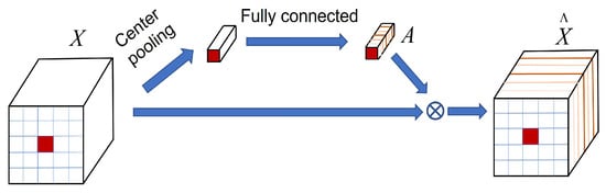
Figure 4. The spectral attention block.

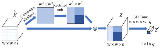
Figure 5. The spatial attention block.

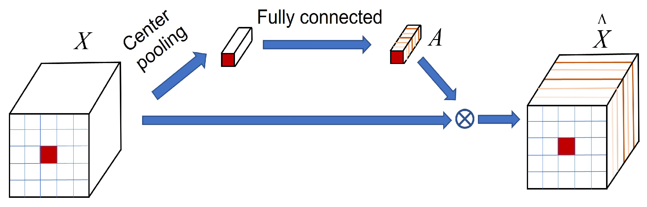
3.3.1. The Spectral Attention Block

Suppressing useless spectral bands and enhancing informative spectral bands can efficiently enhance classification performance [49]. Therefore, we built a spectral attention block (Figure 4) based on a center pooling layer and a fully connection layer. It could generate an attention weight vector to recalibrate spectral features of input cube. The calculation of attention weighting A can be represented as

$$A=ReLU\left(W_{spe}\times Center\left(X_i\right)+b_{spe}\right)$$

(6)

$${\stackrel{\wedge }{X}}_i=A\otimes X_i$$

(7)

where $X_i$ is the i-th feature, $A_i$ is the band weights for the input $X_i$. $W_{spe}$ is the fully connected weight parameters, $b_{spe}$ is the bias, ⊗ denotes the multiplication. The spectral attention features ${\stackrel{\wedge }{X}}_i$ represents the recalibrated $X_i$, which can enhance informative spectral bands and suppress useless spectral bands.

3.3.2. The Spatial Attention Block

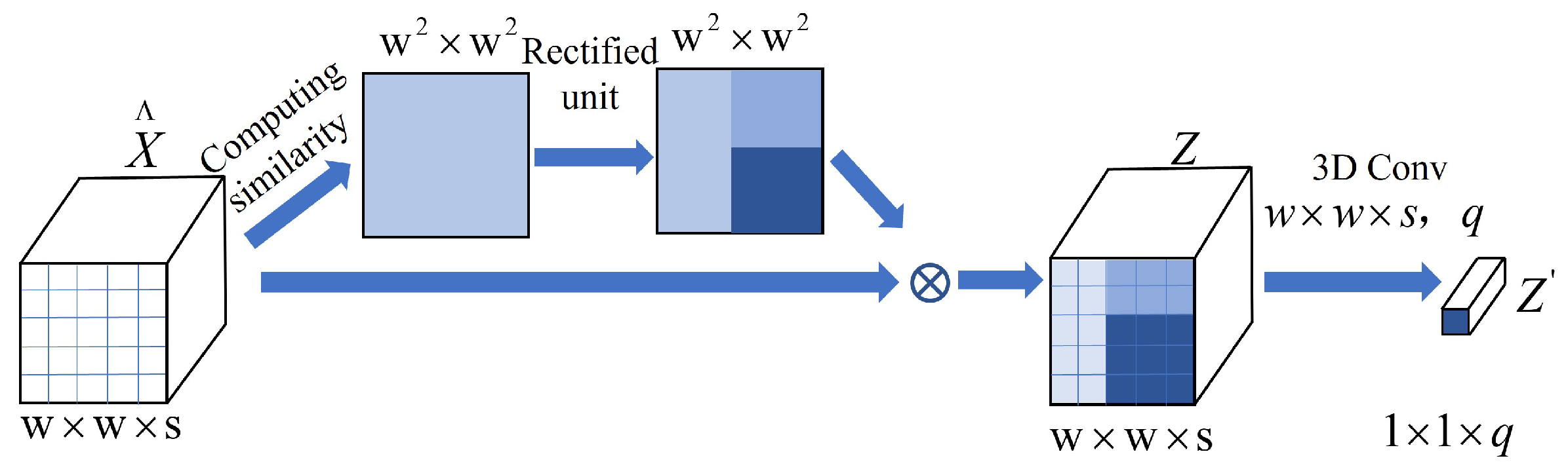
The $\stackrel{\wedge }{X}\in R^{w\times w\times s}$ contains rich spatial information. To further enhance useful spatial features and avoid the interference of useless features, a spatial attention block (Figure 5) was designed to adaptively aggregate the useful spatial features according to the correlation between different pixels. The correlation $S_{ij}\in R^{w^2\times w^2}$ can be calculated as:

$$S_{ij}\left(m,n\right)=\sum \stackrel{\wedge }{X}\left(i,j\right)\otimes \stackrel{\wedge }{X}\left(m,n\right)$$

(8)

A large value of $S_{ij}\left(m,n\right)$ indicates that the correlation between $\stackrel{\wedge }{X}\left(i,j\right)$ and $\stackrel{\wedge }{X}\left(m,n\right)$ is high. This operation can aggregate spatial features of similar pixels and avoid interference from dissimilar pixels. To further enhance the attention weights of similar pixels, we designed a rectified unit $\sigma \left(·\right)$ based on exponential function, which is formulated as:

$$\sigma \left(x\right)=\left\{\begin{array}{c}\hfill e^x,x\ge v·max\left(S_{ij}\right)\\ \hfill e^{\epsilon },x<v·max\left(S_{ij}\right)\end{array}\right.$$

(9)

where v is the ratio of the maximum value of $S_{ij}$. $\epsilon$ is set to $-20$ that makes the attention weight close to 0.

Eventually, the softmax was used to normalize the rectified correlation to generate the spatial attention weight values. Therefore, the spectral-spatial attention features $Z\in R^{w\times w\times s}$ can be expressed as:

$$Z=\sum _{1\le m,n\le w}softmax\left(\sigma \left(S_{ij}\left(m,n\right)\right)\right)\otimes \stackrel{\wedge }{X}\left(m,n\right)$$

(10)

To conveniently calculate the loss between the spectral-spatial attention features of the source domain and target domain, we adopted a 3D convolution layer ($w\times w\times s,q$) to obtain classification features vector $Z^{\prime }\in R^{1\times 1\times q}$.

3.4. The FSL and Multiple Loss Module

In the SSDA, FSL is conducted in source domain and target domain alternately. This can discover transferable knowledge in the source domain and learn individual knowledge to the target domain simultaneously. In particular, the FSL method is shown in Figure 6. Taking a C-way K-shot task of source domain data as an example, we randomly selected C classes from the source domain, and selected K samples for these C classes, respectively, so that there were $C\times K$ samples in total, and used these samples to form a support set $S={\left\{\left(x_i,y_i\right)\right\}}_{i=1}^{C\times K}$. Then, we selected N remaining samples from these C classes, a total of $C\times N$ samples to form the query set $Q={\left\{\left(x_j,y_j\right)\right\}}_{j=1}^{C\times N}$. The support set samples and query set samples were first passed through the mapping layer ($M^s$) to reduce dimensionality. Further, we adopted the spectral-spatial module to learn spectral-spatial features. Finally, a domain attention module was designed to learn useful spectral-spatial features.

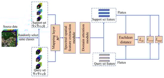
Figure 6. 3-way, 1-shot few-shot learning task.

Moreover, the source domain and the target domain may come from different HSI datasets. To alleviate domain adaptation issue, we designed a multiple loss module consisted of the few-shot loss, coral loss, and mmd loss. In particular, the few-shot loss was utilized to minimize the cross entropy between the predicted labels and the truth labels. The coral loss was utilized to minimize the difference in learned feature covariances between source domain and target domain. The mmd loss was utilized to minimize the distribution discrepancy between source domain and target domain.

3.4.1. The Few-Shot Loss

For a query sample $x_j$, the predicted probability can be written as:

$$P\left(y_j=l\mid x_j\in Q\right)=\frac{exp\left(-d\left(F_{\omega }\left(x_j\right),z_l^{\prime }\right)\right)}{{\sum }_{l=1}^{C}exp\left(-d\left(F_{\omega }\left(x_j\right),z_l^{\prime }\right)\right)}$$

(11)

where $d(·)$ represents the Euclidean distance, $F_{\omega }(·)$ denotes the parameters $\omega$ of the mapping layer, domain attention module, and spectral-spatial module, $z_l^{\prime }$ denotes the features vector of the $l_{th}$ class in the support set S, C represents the number of classes, $x_j$ represents sample of the query set and $y_j$ denotes the corresponding label.

Based on the cross entropy formula, the few-shot classification loss of a source episode can be written as:

$$L_{fsl}^s=-\sum _{\left(x,y\right)\in Q_s}log{P}_w\left(y=l|x\right)$$

(12)

where $Q_s$ represents the query samples from source domain.

Likewise, the classification loss of a target episode can be represented as:

$$L_{fsl}^t=-\sum _{\left(x,y\right)\in Q_t}log{P}_w\left(y=l|x\right)$$

(13)

where $Q_t$ represents the query set samples from target domain data.

3.4.2. The Coral Loss

In this work, we adopted the coral loss to better represent the feature covariances difference between source domain and target domain and improve the classification performance. In detail, given source domain training examples $D_s=\left\{Z_i^s\right\},Z_i^s\in R^d$ with labels $L_s=\left\{y_i\right\},i\in \{1,\dots ,L\}$. The unlabeled target domain data can be represented as $D_t=\left\{Z_i^t\right\},Z_i^t\in R^d$, where $Z_i^s$ and $Z_i^t$ are the feature vectors obtained from the source domain and target domain data through the SSDA, respectively. The number of source domain samples and target domain samples were set as $n_s$ and $n_t$ respectively. To be more specific, we defined $D_s^{ij}$ and $D_t^{ij}$ as the j-th dimension of the i-th source domain data sample and target domain data sample separately. Further, we denoted $C_s$ and $C_t$ as the feature covariance matrices of source domain and target domain separately, which can be computed by

$$C_s=\frac{1}{n_s-1}\left(D_s^{\top }{D}_s-\frac{1}{n_s}{\left({\mathbf{1}}^{\top }{D}_s\right)}^{\top }\left({\mathbf{1}}^{\top }{D}_s\right)\right)$$

(14)

$$C_t=\frac{1}{n_t-1}\left(D_t^{\top }{D}_t-\frac{1}{n_t}{\left({\mathbf{1}}^{\top }{D}_t\right)}^{\top }\left({\mathbf{1}}^{\top }{D}_t\right)\right)$$

(15)

where 1 is a unit column vector and the value of all elements in it is 1.

The coral loss can be represented as the second-order statistics distance between $C_s$ and $C_t$:

$$L_{coral}=\frac{1}{4d^2}{∥C_s-C_t∥}_F^2$$

(16)

where ${\parallel ·\parallel }_F^2$ represents the squared matrix Frobenius norm.

3.4.3. The Maximum Mean Discrepancy

The maximum mean discrepancy (mmd) is an efficient nonparametric difference metric, which is widely used to measure the distribution distance.

$$L_{mmd}\left(Z_s,Z_t\right)={∥\frac{1}{n_s}\sum _{i=1}^{n_s}\varphi \left(z_i^s\right)-\frac{1}{n_t}\sum _{j=1}^{n_t}\varphi \left(z_j^t\right)∥}_H^2$$

(17)

This formula can calculate the mean discrepancy between source domain and target domain. The smaller the value of the mmd, the more similar the two domains, and vice versa.

4. Results

To prove the validity of the SSDA, we conducted extensive comparative experiments on the four commonly used HSI datasets, including the Chikusei, the Salinas, the University of Pavia (UP), the Indian Pines (IP), and a new Huoshaoyun mineral exploration dataset that was captured by the GF-5 satellite. In particular, the Chikusei was utilized as the source domain. Other datasets were utilized as the target domain. Three standard evaluation indicators included overall accuracy (OA) and average accuracy (AA), and kappa coefficients (K) were utilized to verify the model performance.

4.1. Experimental Datasets

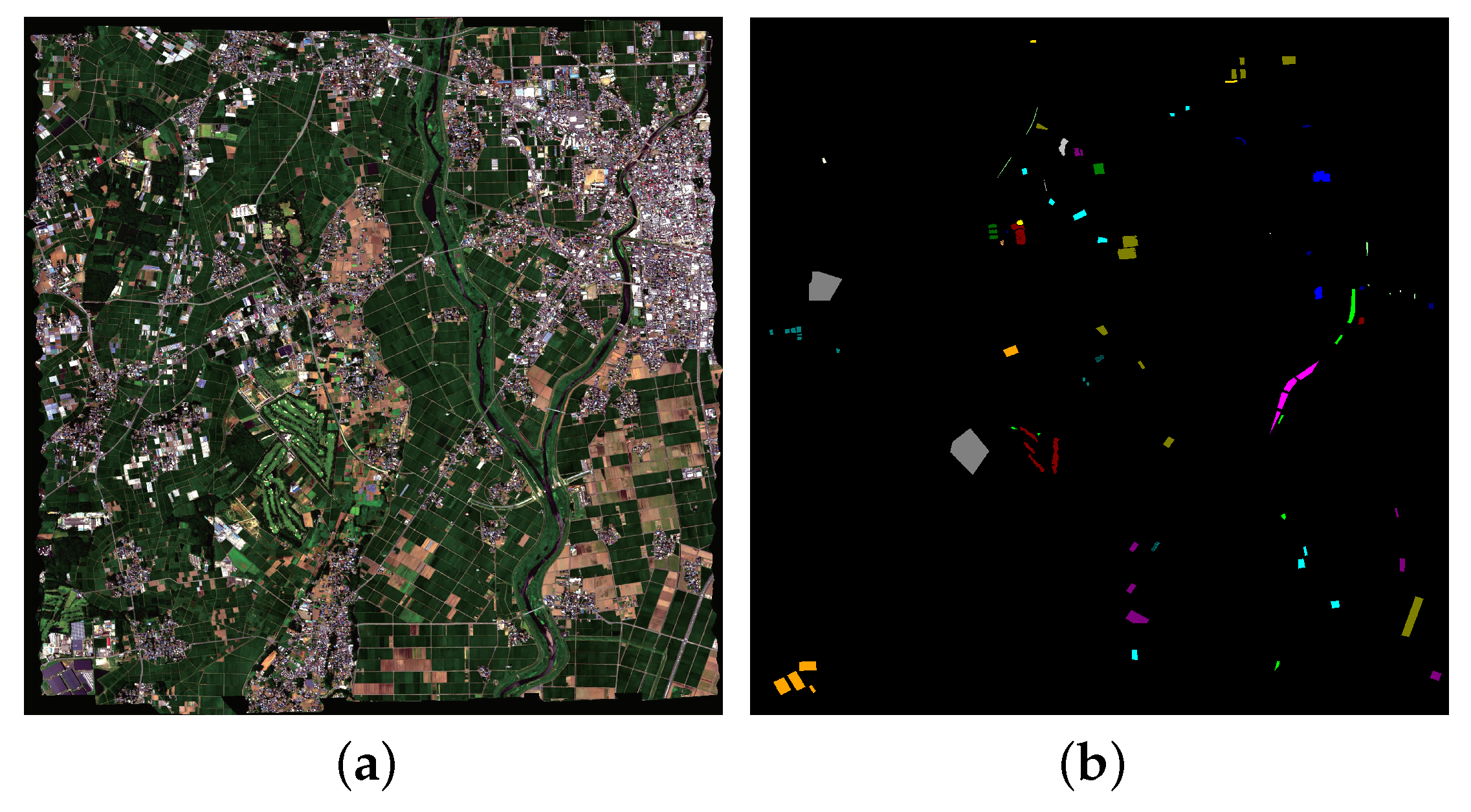
The Chikusei dataset: The Chikusei dataset [50] contains 128 bands, ranging from 363 to 1018 nm, and the size and the spatial resolution are $2517\times 2335$ and 2.5 m, respectively. It has 19 classes, including urban and rural areas. Figure 7 shows the false color image and ground truth of the Chikusei dataset. Different colors in Figure 7b represent different classes.

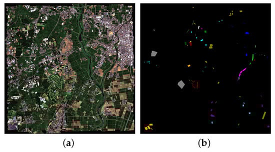
Figure 7. (a) False color image of the Chikusei dataset, (b) The ground truth of the Chikusei dataset.

The Salinas dataset: The Salinas Scene dataset has 512 × 217 pixels with 204 bands. It has 16 classes and a spatial resolution of 3.7 m.

The UP dataset: The University of Pavia (UP) has $610\times 340$ pixels with 103 bands. It has 9 classes.

The IP dataset: The Indian Pines dataset includes 16 classes with a wavelength scope of 400 to 2500 nm. It has 145 × 145 pixels with 200 bands.

The Huoshaoyun dataset: The Huoshaoyun dataset was captured by GF-5 satellite in Xinjiang province, China. The size of the entire dataset is $150\times 150$. It contains 9 lithology classes with 164 bands, ranging from 390–2513 nm, which is mainly used for mineral exploration. Most of the classes are rocks with similar characteristics, and thus their distribution is disorderly and staggered, which leads to greater difficulty classifying Huoshaoyun dataset. Table 1, Table 2, Table 3, Table 4 and Table 5 describe the detailed information of each class on Chikusei, Salinas, UP, IP, and Huoshaoyun datasets, respectively.

Table 1. Class information for the Chikusei dataset (Chikusei).

Order Number	Classification	Number of Samples
1	Water	2845
2	Bare soil (school)	2859
3	Bare soil (park)	286
4	Bare soil (farmland)	48,525
5	Nature plants	4297
6	Weeds in farmland	1108
7	Forest	20,516
8	Grass	6515
9	Rice field (grown)	13,369
10	Rice field (first stage)	1268
11	Row crops	5961
12	Plastic house	2193
13	Manmade (non-dark)	1220
14	Manmade (dark)	7664
15	Manmade (blue)	431
16	Manmade (red)	222
17	Manmade grass	1040
18	Asphalt	801
19	Paved ground	145
	Total	77,592

Table 2. Class information for the Salinas dataset (Salinas).

Order Number	Classification	Number of Samples
1	Brocoli_green_weeds_1	2009
2	Brocoli_green_weeds_2	3726
3	Fallow	1976
4	Fallow_rough_plow	1394
5	Fallow_smooth	2678
6	Stubble	3959
7	Celery	3579
8	Grapes_untrained	11,271
9	Soli_vinyard_develop	6203
10	Corn_senesced_green_weeds	3278
11	Lettuce_romaine_4wk	1068
12	Lettuce_romaine_5wk	1927
13	Lettuce_romaine_6wk	916
14	Lettuce_romaine_7wk	1070
15	Vinyard_untrained	7268
16	Vinyard_vertical_trellis	1807
	Total	54,129

Table 3. Class information for the University of Pavia dataset (UP).

Order Number	Classification	Number of Samples
1	Asphalt	6631
2	Meadows	18,649
3	Gravel	2099
4	Trees	3064
5	Painted metal sheets	1345
6	Bare soil	5029
7	Bitumen	1330
8	Self-blocking bricks	3692
9	Shadow	947
	Total	42,776

Table 4. Class information for the Indian Pines dataset (IP).

Order Number	Classification	Number of Samples
1	Alfalfa	46
2	Corn–notill	1428
3	Corn–mintill	830
4	Corn	237
5	Grass–pasture	483
6	Grass–tree	730
7	Grass–pasture–mowed	28
8	Hay–windrowed	478
9	Oats	20
10	Soybean–notill	972
11	Soybean–mintill	2455
12	Soybean–clean	593
13	Wheat	205
14	Woods	1265
15	Buildings–Grass–Trees–Dribes	386
16	Stone–Steel–Towers	93
	Total	10,249

Table 5. Class information for the Huoshaoyun dataset (Huoshaoyun).

Order Number	Classification	Number of Samples
1	Sandstone-1	2424
2	Sandstone-2	573
3	Sandstone-3	1826
4	Sandstone-4	897
5	Sandstone-5	779
6	Sandstone-6	1936
7	Sandstone-7	811
8	Sandstone-8	3438
9	Sandstone-9	4391
	Total	17,075

4.2. Framework Setting

4.2.1. Basic Settings

In this study, we built the SSDA via using Pytorch as a backend. In the SSDA, the data cube with the spatial size of $9\times 9$ was utilized as the input to start the training. Before training the SSDA framework, some important parameters needed to be configured. We used the Adam optimizer as stochastic optimization and the initial learning rate was set to 0.001. We set the number of training epochs to 10,000. Every epoch was a C-way, K-shot classification task. Here, C is the number of classes of the target domain dataset. For example, C was set to 9 in the UP and Huoshaoyun datasets, and C was set to 16 in the Salinas and IP datasets. The K was set to 1 in the support set, which meant that one sample was randomly selected at a time and sent to the model for training. At the same time, K was set to 19 in the query set because of the theory that the higher the sample number per class is in the test dataset, the higher the accuracy of predicting samples of each class [42,43].

4.2.2. The Input Spatial Size

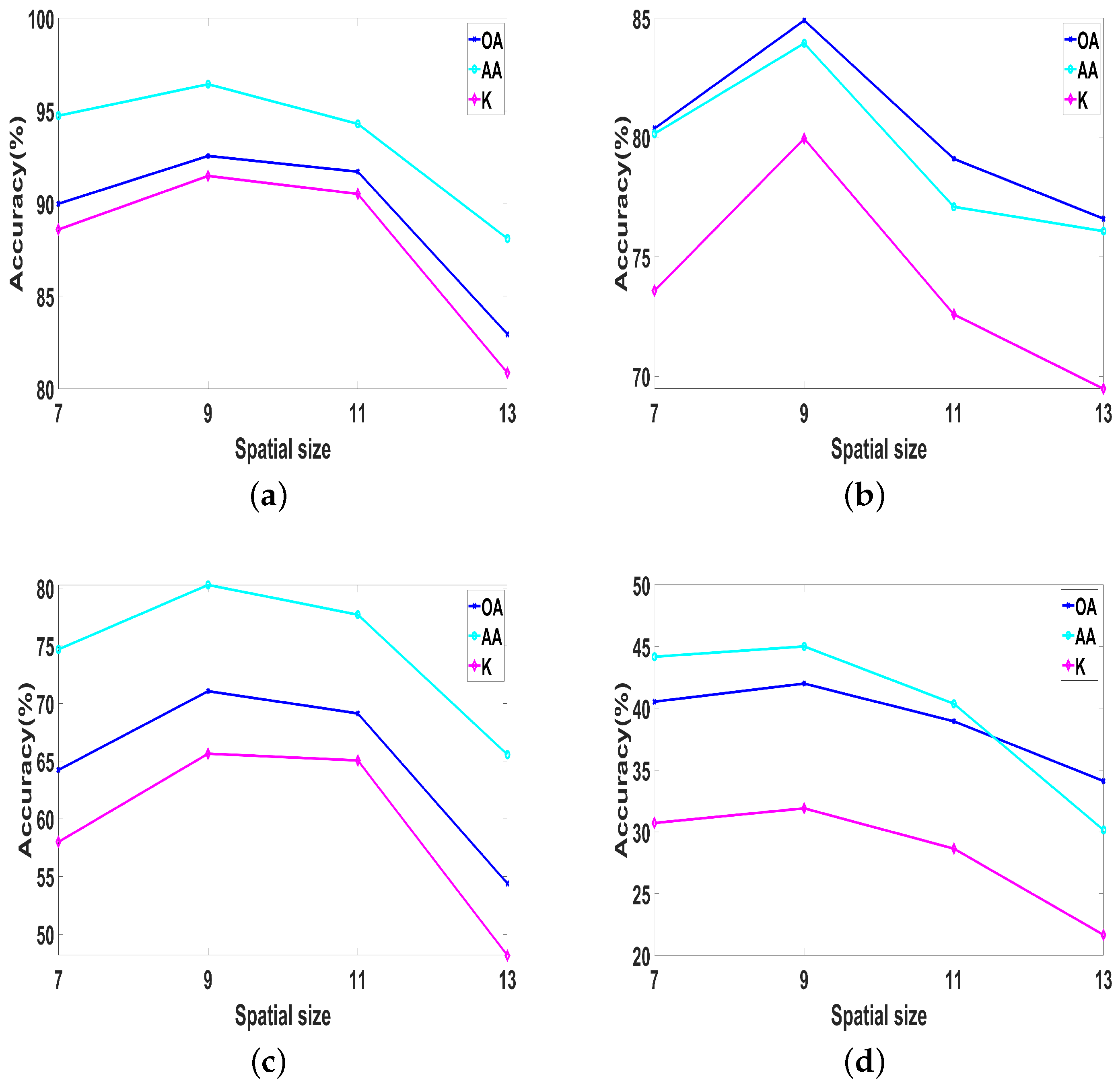
To explore the impact of input sample spatial size on classification results, we designed a controlled experiment, which set the spatial size of input samples to $7\times 7, 9\times 9$, $11\times 11$, $13\times 13$, respectively, and trained on four datasets. As shown in Figure 8, on the four datasets (Salinas, UP, IP, and Huoshaoyun), when the spatial size of samples was set to $9\times 9$, three evaluation indicators (OA, AA, K) achieved the highest value. Therefore, we set the spatial size of the sample to $9\times 9$.

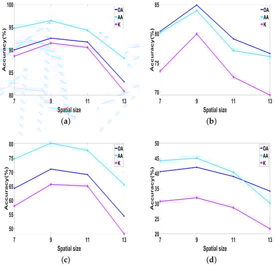
Figure 8. The OA, AA, and K for varying spatial size samples on Salinas, UP, IP, Huoshaoyun datasets. (a) Salinas; (b) UP; (c) IP; (d) Huoshaoyun.

4.2.3. Learning Rate

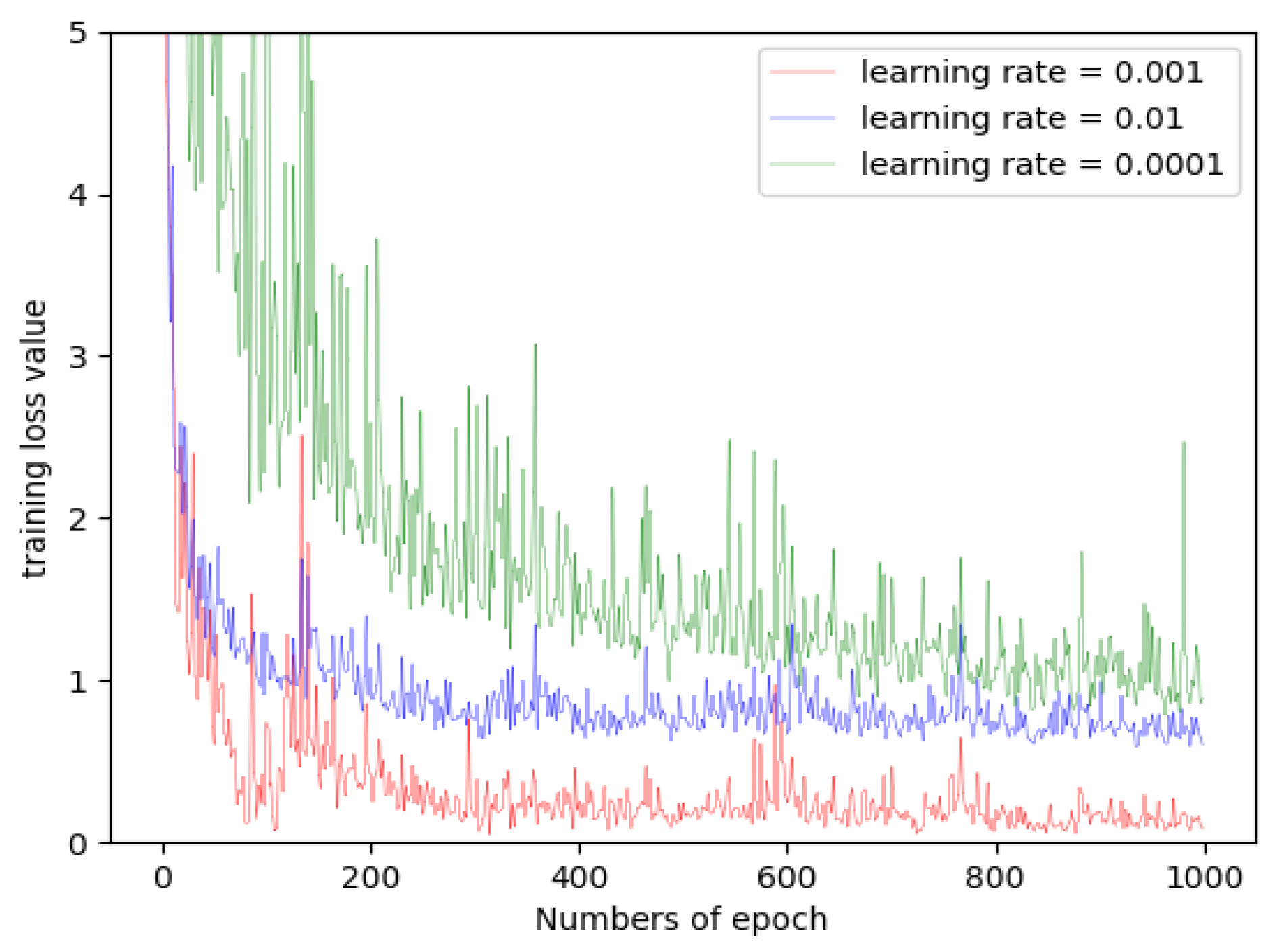
The learning rate is a critical hyperparameter in the training process, determining whether the multiple loss module can converge to a local minimum. To analyze the effect of learning rate on the SSDA framework, we set the learning rate to 0.01, 0.001, and 0.0001, separately. Taking the Salinas data as an example, we display the training loss curves at different learning rates in Figure 9. It is easy to see that at a larger learning rate, it is difficult to make the multiple loss module converge. When the learning rate is set to 0.001, the multiple loss module obtains the best convergence effect. Therefore, the learning rate of the SSDA was set to 0.001.

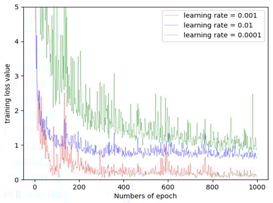
Figure 9. Training loss values with different learning rates on the Salinas data.

4.3. Compared with Other Methods

In this part, we compare the SSDA to other learning-based methods, such as 3D-DenseNet [51], SSRN [52], existing FSL methods DFSL + NN [42], DFSL + SVM [42] and deep relation network RN-FSC [43], and DCFSL [53]. For two supervised methods (3D-DenseNet and SSRN methods), since the training and test classes need to be the same, we randomly selected some labeled samples from the target domain data to train the classifier. We set the number of labeled samples per class to five, and the rest of the target domain data was used as test data. However, for the few-shot learning (FSL) methods (DFSL + SVM, DFSL + NN, RN-FSC, and DCFSL), it is mainly to learn transferable knowledge through source domain data to form a metric space. For the above methods, the classes between two domains may be different, so the source domain data and five labeled samples for each class of target domain data were used for training. All experiments were conducted ten times to remove the impact of random sampling. In particular, OA, AA, and Kappa data are given as mean ± standard deviation and the highest accuracies are shown in bold.

Table 6, Table 7, Table 8 and Table 9 display the OA, AA, K, and the classification accuracy of each class on the four HSI datasets. The SSDA achieves the highest OA, AA, and K than all other methods on the four HSI datasets. This is because our SSDA can extract discriminative and domain invariance spectral-spatial features, which can effectively improve the classification performance with the limited labeled samples.

Table 6. Overall accuracy (OA), average accuracy (AA), and kappa coefficient (K) for each HSI class on the Salinas dataset.

Method	3D-DenseNet	SSRN	DFSL + NN	DFSL + SVM	RN-FSC	DCFSL	SSDA
OA	49.43 ± 4.19	86.39 ± 2.68	87.05 ± 0.83	86.95 ± 1.30	84.11 ± 1.36	89.34 ± 2.19	92.57 ± 0.49
AA	53.53 ± 4.32	93.24 ± 1.29	91.01 ± 0.66	90.08 ± 1.44	88.83 ± 2.07	94.04 ± 1.14	96.44 ± 0.51
Kappa	60.01 ± 3.84	84.95 ± 2.90	85.63 ± 0.91	85.51 ± 1.42	82.38 ± 1.53	88.17 ± 2.40	91.49 ± 0.56
1	35.58	97.55	95.63	73.92	97.47	99.40	99.75
2	72.84	98.97	99.09	96.85	99.47	99.76	98.58
3	40.99	92.47	94.01	96.28	85.05	91.96	98.88
4	51.74	96.50	99.54	99.11	98.75	99.55	100
5	62.60	94.20	90.58	80.72	83.45	92.70	94.13
6	81.16	99.28	98.47	91.63	96.73	99.52	100
7	70.96	99.98	99.81	97.73	99.61	98.88	99.61
8	56.61	86.90	77.74	82.33	72.11	74.57	78.29
9	92.02	99.64	91.13	94.44	88.35	99.59	100
10	67.26	92.01	60.98	80.96	70.53	86.42	92.18
11	55.07	95.86	95.99	93.38	90.03	96.61	99.62
12	62.27	99.15	93.13	97.94	93.15	99.93	99.95
13	73.61	89.24	99.34	95.79	98.54	99.30	99.23
14	28.73	95.15	98.06	98.87	96.43	98.85	99.53
15	48.83	55.97	77.54	71.13	70.18	75.38	84.00
16	59.97	98.91	85.05	90.57	82.39	92.22	99.33

Table 7. Overall accuracy (OA), average accuracy (AA), and kappa coefficient (K) for each HSI class on the University of Pavia (UP) dataset.

Method	3D-DenseNet	SSRN	DFSL + NN	DFSL + SVM	RN-FSC	DCFSL	SSDA
OA $\left(\%\right)$	45.21 ± 8.32	76.26 ± 5.78	77.75 ± 1.16	79.63 ± 1.09	80.19 ± 2.18	83.65 ± 1.77	84.91 ± 2.62
AA $\left(\%\right)$	56.51 ± 8.18	79.51 ± 3.21	77.57 ± 0.31	76.41 ± 1.39	77.12 ± 0.84	83.77 ± 1.74	83.95 ± 0.28
K $\left(\%\right)$	58.54 ± 4.02	70.56 ± 6.69	71.11 ± 1.22	73.05 ± 1.60	73.73 ± 2.79	78.70 ± 2.01	79.96 ± 0.20
1	74.91	91.84	69.19	73.43	68.55	82.20	78.81
2	73.98	95.13	84.63	89.25	93.44	87.74	87.88
3	28.63	55.23	57.47	48.09	49.81	67.46	68.24
4	79.27	78.02	89.99	84.72	92.15	93.16	93.85
5	76.90	98.34	100	99.65	99.43	99.49	99.70
6	27.93	53.56	71.23	67.81	57.99	77.32	91.34
7	18.29	60.07	70.62	64.48	70.04	81.18	73.96
8	60.55	85.34	58.13	67.37	63.48	66.73	61.84
9	86.37	98.08	96.92	92.92	99.19	98.66	99.89

Table 8. Overall accuracy (OA), average accuracy (AA), and kappa coefficient (K) for each HSI class on the Indian Pines (IP) dataset.

Method	3D-DenseNet	SSRN	DFSL + NN	DFSL + SVM	RN-FSC	DCFSL	SSDA
OA $\left(\%\right)$	41.61 ± 1.26	61.36 ± 0.49	59.65 ± 0.63	61.69 ± 1.85	58.17 ± 0.02	66.81 ± 2.37	71.06 ± 0.64
AA $\left(\%\right)$	47.67 ± 1.31	59.75 ± 0.20	72.24 ± 0.42	73.05 ± 0.84	69.90 ± 0.40	77.89 ± 0.86	80.27 ± 1.63
K $\left(\%\right)$	43.06 ± 1.79	56.91 ± 0.48	54.55 ± 0.52	56.78 ± 1.90	52.52 ± 0.14	62.64 ± 0.86	65.64 ± 0.29
1	47.47	18.38	96.74	96.75	96.34	95.37	95.12
2	35.69	64.79	38.65	36.38	46.13	43.26	28.25
3	26.34	27.65	42.79	38.34	40.61	43.26	56.48
4	20.33	26.97	68.10	77.16	58.62	80.60	96.98
5	39.97	80.76	71.20	73.92	64.96	72.91	79.92
6	84.60	86.87	76.18	86.25	69.45	87.96	87.72
7	12.16	32.24	100	97.10	100	99.57	100
8	78.28	100	74.84	81.82	77.70	86.26	99.37
9	13.29	57.69	100	75.56	100	99.33	100
10	33.89	59.69	47.98	52.22	25.49	62.44	62.87
11	62.63	70.87	57.95	59.96	65.51	62.75	77.02
12	29.23	45.00	38.21	36.56	27.13	48.72	39.12
13	53.41	88.29	97.50	98.00	99.75	99.35	99.50
14	75.40	97.18	83.44	84.63	76.35	85.40	91.90
15	55.64	36.64	62.29	74.10	70.34	66.69	71.13
16	20.63	60.98	100	100	100	97.61	98.86

Table 9. Overall accuracy (OA), average accuracy (AA), and kappa coefficient (K) for each HSI class in the Huoshaoyun dataset.

Method	3D-DenseNet	SSRN	DFSL + NN	DFSL + SVM	RN-FSC	DCFSL	SSDA
OA $\left(\%\right)$	25.04 ± 0.64	40.85 ± 1.37	37.83 ± 2.54	40.81 ± 2.74	30.54 ± 1.70	39.58 ± 0.58	44.37 ± 0.36
AA $\left(\%\right)$	28.30 ± 0.78	31.16 ± 1.33	33.67 ± 3.16	35.84 ± 2.35	32.15 ± 2.91	43.10 ± 1.49	49.87 ± 0.45
K $\left(\%\right)$	14.48 ± 0.94	32.54 ± 0.62	27.05 ± 2.88	30.38 ± 2.92	20.75 ± 2.53	29.97 ± 0.52	34.66±0.42
1	32.63	44.72	55.77	57.12	59.81	44.61	44.56
2	32.97	4.22	28.28	35.76	52.40	69.72	96.86
3	22.53	28.19	29.33	31.48	28.33	28.67	30.97
4	28.34	24.97	29.07	26.13	11.48	62.11	82.51
5	15.86	5.41	12.42	17.79	6.92	48.45	47.55
6	23.03	32.16	20.71	19.87	21.29	19.99	32.37
7	12.78	6.71	15.01	17.76	7.30	39.95	38.46
8	37.91	61.30	59.89	61.04	43.50	16.57	12.09
9	48.66	72.79	52.57	55.64	58.29	57.84	63.45

In detail, on the Salinas dataset (Table 6), the proposed SSDA increases OA, AA, and K by $3.23\%$, $2.40\%$ and $3.32\%$ than the state-of-the-art DCFSL method, respectively. Meanwhile, it has obtained the highest accuracy in 11 of the 16 classes (class 1, 3, 4, 6, 9, 10, 11, 12, 14, 15, 16). On the UP dataset (Table 7), compared with the state-of-the-art DCFSL method, our framework improves OA, AA, and K by $1.26\%$, $0.18\%$ and $1.26\%$, respectively. Meanwhile, it has obtained the highest accuracy in 3 of the 9 classes (class 4, 6, 9). On the IP dataset (Table 8), the proposed SSDA increases OA, AA, and K by $4.25\%$, $2.38\%$, $3.00\%$ than the state-of-the-art DCFSL method respectively. Meanwhile, it has achieved the highest accuracy in 6 of the 16 classes (class 3, 4, 7, 9, 10, 11). Especially, on the Huoshaoyun dataset (Table 9), compared with state-of-the-art DCFSL method, our framework improves OA, AA, and K by $4.79\%$, $6.77\%$ and $4.69\%$ respectively. Meanwhile, it has obtained the highest accuracy in 4 of the 9 classes (class 2, 3, 6, 7).

To sum up, by comparing the FSL methods and deep learning methods, we found that FSL methods have higher classification performance than the deep learning-based methods. This is because the meta-learning strategy in the FSL methods can transfer the classification knowledge from source domain to target domain, which can improve the classification accuracy on the target domain.

4.4. Classification Maps Visualization

To further visually verify the validity of the SSDA, we have drawn the classification maps obtained from the Salinas, UP, IP and Huoshaoyun datasets using different methods in Figure 10, Figure 11, Figure 12 and Figure 13 respectively.

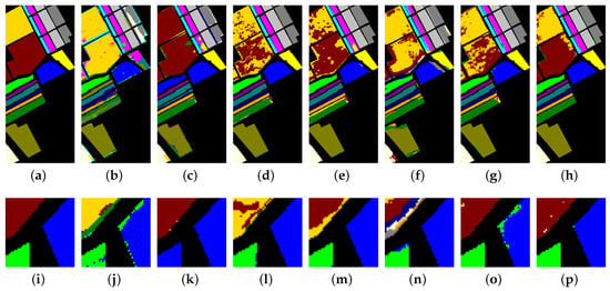
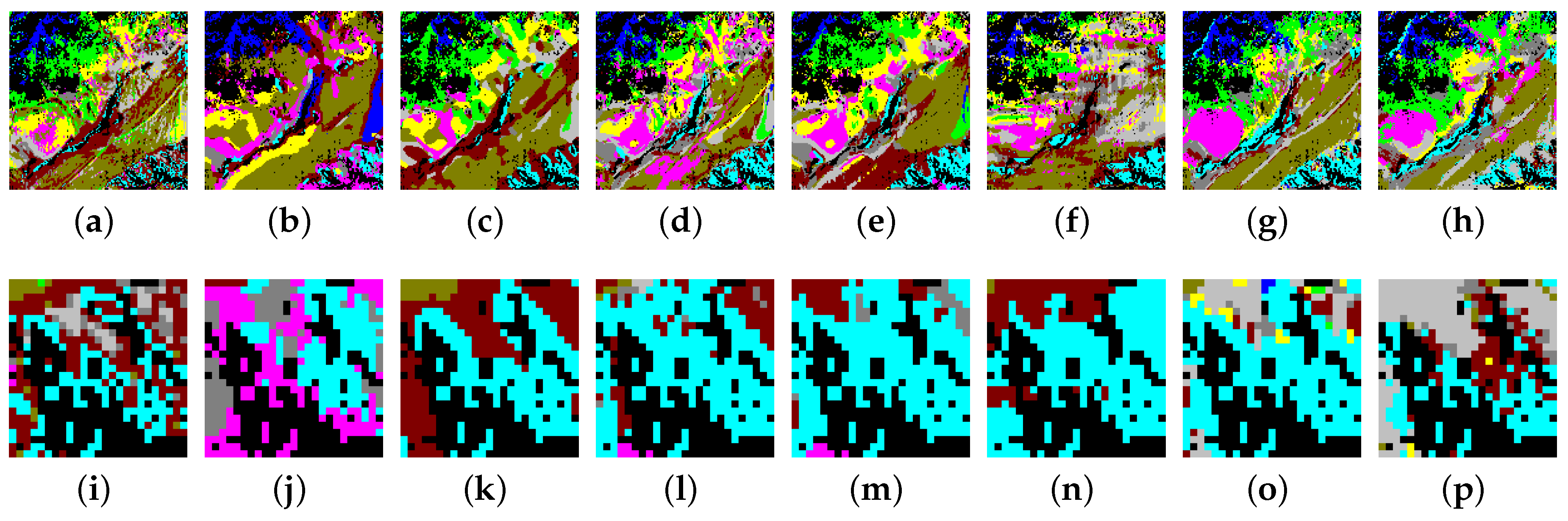
Figure 10. Classification maps produced by different methods on the Salinas dataset. (a) Ground truth map; (b) 3D-DenseNet; (c) SSRN; (d) DFSL + NN; (e) DFSL + SVM; (f) RN-FSC; (g) DCFSL; (h) Our model; (i) The zoom in an area of ground truth map; (j) The zoom in an area of 3D-DenseNet; (k) The zoom in an area of SSRN; (l) The zoom in an area of DFSL + NN; (m) The zoom in an area of DFSL + SVM; (n) The zoom in an area of RN-FSC; (o) The zoom in an area of DCFSL; (p) The zoom in an area of our model.

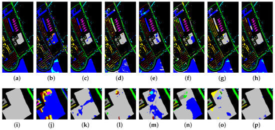
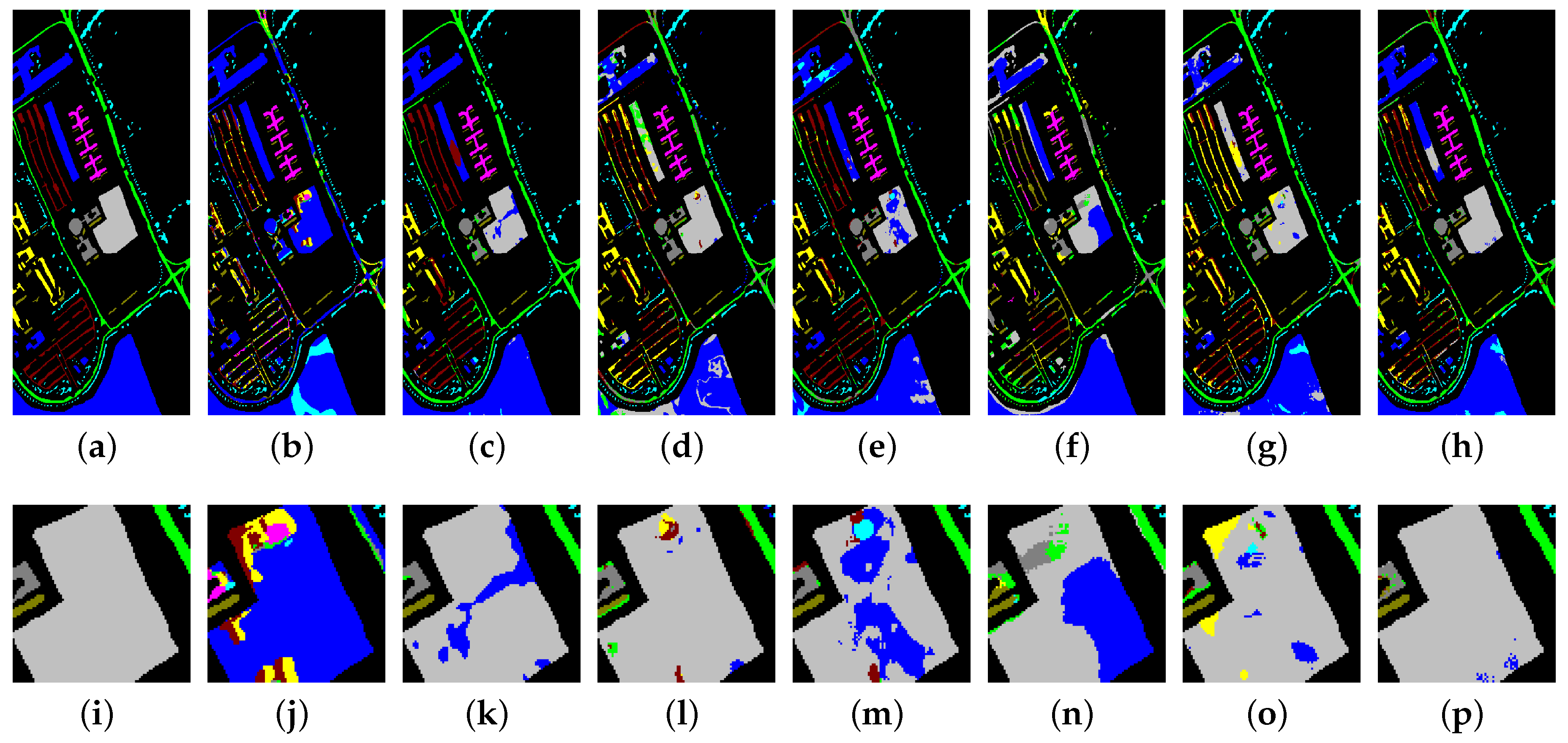
Figure 11. Classification maps produced by different methods on the UP dataset. (a) Ground truth map; (b) 3D-DenseNet; (c) SSRN; (d) DFSL + NN; (e) DFSL + SVM; (f) RN-FSC; (g) DCFSL; (h) Our model; (i) The zoom in an area of ground truth map; (j) The zoom in an area of 3D-DenseNet; (k) The zoom in an area of SSRN; (l) The zoom in an area of DFSL + NN; (m) The zoom in an area of DFSL + SVM; (n) The zoom in an area of RN-FSC; (o) The zoom in an area of DCFSL; (p) The zoom in an area of our model.

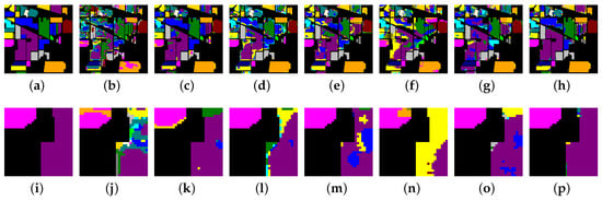
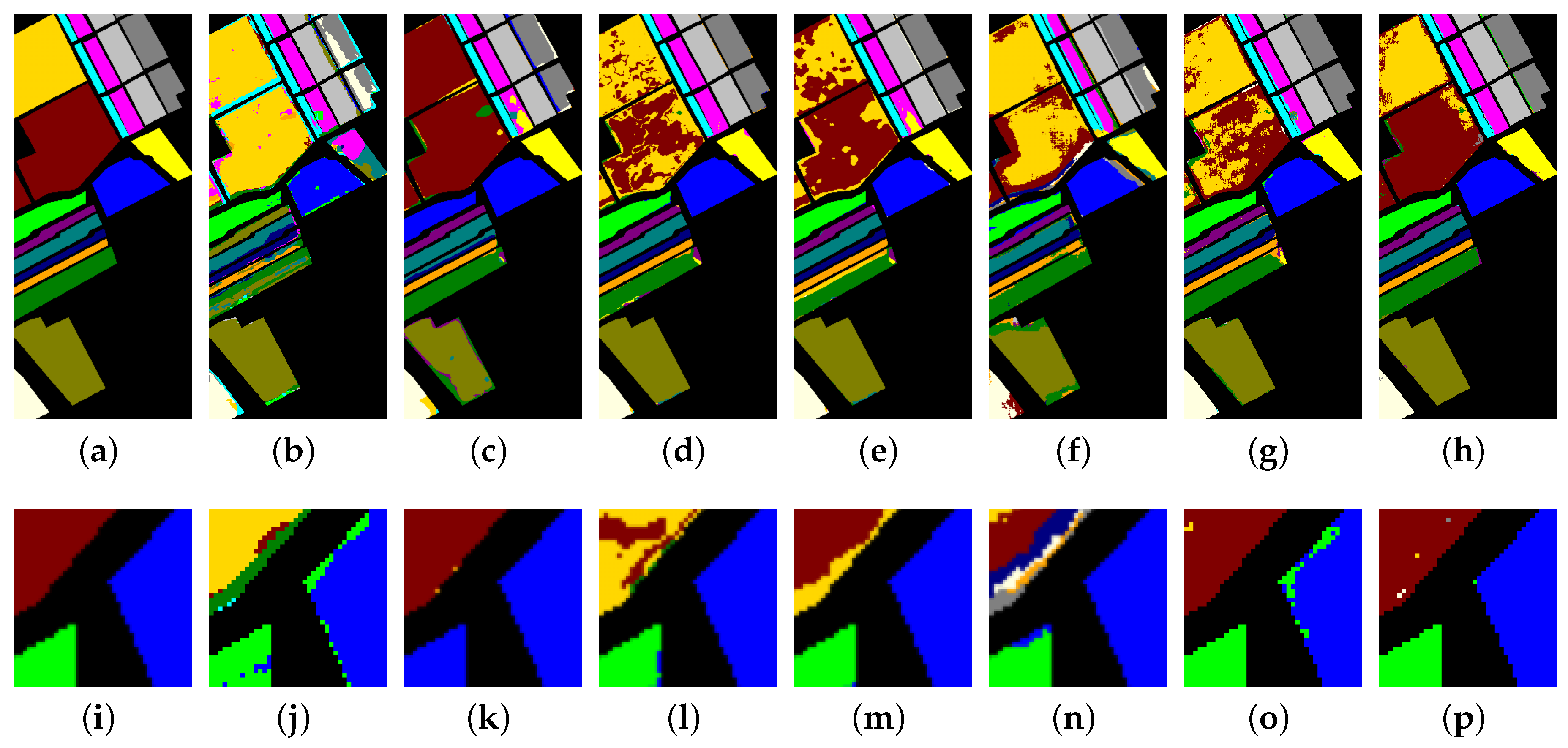
Figure 12. Classification maps produced by different methods on the IP dataset. (a) Ground truth map; (b) 3D-DenseNet; (c) SSRN; (d) DFSL + NN; (e) DFSL + SVM; (f) RN-FSC; (g) DCFSL; (h) Our model; (i) The zoom in an area of ground truth map; (j) The zoom in an area of 3D-DenseNet; (k) The zoom in an area of SSRN; (l) The zoom in an area of DFSL + NN; (m) The zoom in an area of DFSL + SVM; (n) The zoom in an area of RN-FSC; (o) The zoom in an area of DCFSL; (p) The zoom in an area of our model.

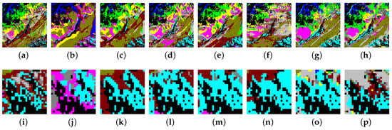
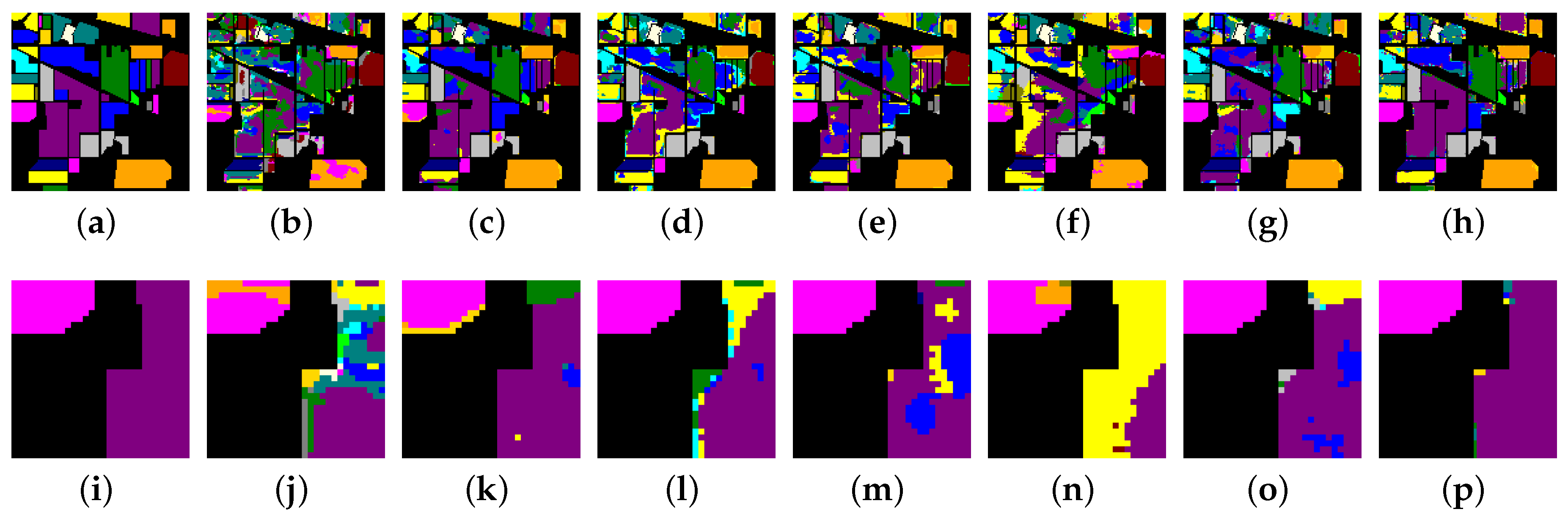
Figure 13. Classification maps produced by different methods on the Huoshaoyun dataset. (a) Ground truth map; (b) 3D-DenseNet; (c) SSRN; (d) DFSL + NN; (e) DFSL + SVM; (f) RN-FSC; (g) DCFSL; (h) Our model; (i) The zoom in an area of ground truth map; (j) The zoom in an area of 3D-DenseNet; (k) The zoom in an area of SSRN; (l) The zoom in an area of DFSL + NN; (m) The zoom in an area of DFSL + SVM; (n) The zoom in an area of RN-FSC; (o) The zoom in an area of DCFSL; (p) The zoom in an area of our model.

As shown in Figure 10, Figure 10a–h display the classification maps of the ground truth, 3D-DenseNet, SSRN, DFSL + NN, DSFL + SVM, RN-FSC, DCFSL, and our method on the Salinas dataset. To compare the classification results in more detail, we perform a region zoom in the middle of these classification maps (Figure 10i–p). Obviously, our method (Figure 10p) can generate more accurate predictions than other methods (Figure 10i–o). On the UP dataset (Figure 11), the classifiaction map (Figure 11p) of our method is the closet to the ground truth (Figure 11i). On the IP dataset (Figure 12), we perform a region zoom in the lower left corner of these classification maps. Our method (Figure 12p) predicts fewer misclassification than other methods (Figure 12i–o). It is likely that on the Huoshaoyun region zoom in the lower right corner of classification maps (Figure 13i–p), our method (Figure 13p) also predicts fewer misclassification than other methods (Figure 13i–o). In conclusion, the classification maps produced by our SSDA are the closest to the ground truth on four datasets.

5. Discussion

5.1. Ablation Study

In this part, we evaluate how the spectral-spatial module, the domain attention module, the few-shot loss, the coral loss, and the mmd loss in our proposed SSDA influence the classification performance. The detailed experimental results with different modules are presented in Table 10 and the highest accuracies are shown in bold.

Table 10. Ablation experiments with different variants on the four HSI datasets.

Datasets	Methods	SSDA without Spectral-Spatial Module	SSDA without Domain Attention Module	SSDA without fsl Loss	SSDA without Coral Loss	SSDA without mmd Loss	SSDA
UP	OA $\left(\%\right)$	81.91	79.57	81.06	81.94	83.17	84.91
	AA $\left(\%\right)$	80.35	79.30	80.92	81.09	81.76	83.95
	K $\left(\%\right)$	76.25	74.05	77.73	78.18	77.85	79.96
Salinas	OA $\left(\%\right)$	91.84	90.98	91.01	91.36	91.76	92.57
	AA $\left(\%\right)$	96.19	94.08	95.33	95.87	96.02	96.44
	K $\left(\%\right)$	90.67	89.70	90.35	90.03	91.13	91.49
IP	OA $\left(\%\right)$	69.39	68.35	68.78	69.11	70.21	71.06
	AA $\left(\%\right)$	80.01	79.04	79.61	78.59	79.23	80.27
	K $\left(\%\right)$	63.84	62.70	63.99	64.21	64.89	65.64
Huoshaoyun	OA $\left(\%\right)$	39.61	39.01	40.82	41.32	41.98	42.70
	AA $\left(\%\right)$	40.83	40.69	42.14	42.39	43.67	45.18
	K $\left(\%\right)$	28.86	28.84	29.58	30.98	31.74	32.73

As shown in Table 10, we designed five SSDA variants: SSDA without spectral-spatial module, SSDA without domain attention module, SSDA without the fsl loss, SSDA without the coral loss, and SSDA without the mmd loss. The detailed classification results are presented in Table 10 on four datasets. The results indicate that our SSDA achieves the best accuracy than other methods, which means that the spectral-spatial module, domain attention module, the few-shot loss, the coral loss, and the mmd loss can improve the classification performance effectively.

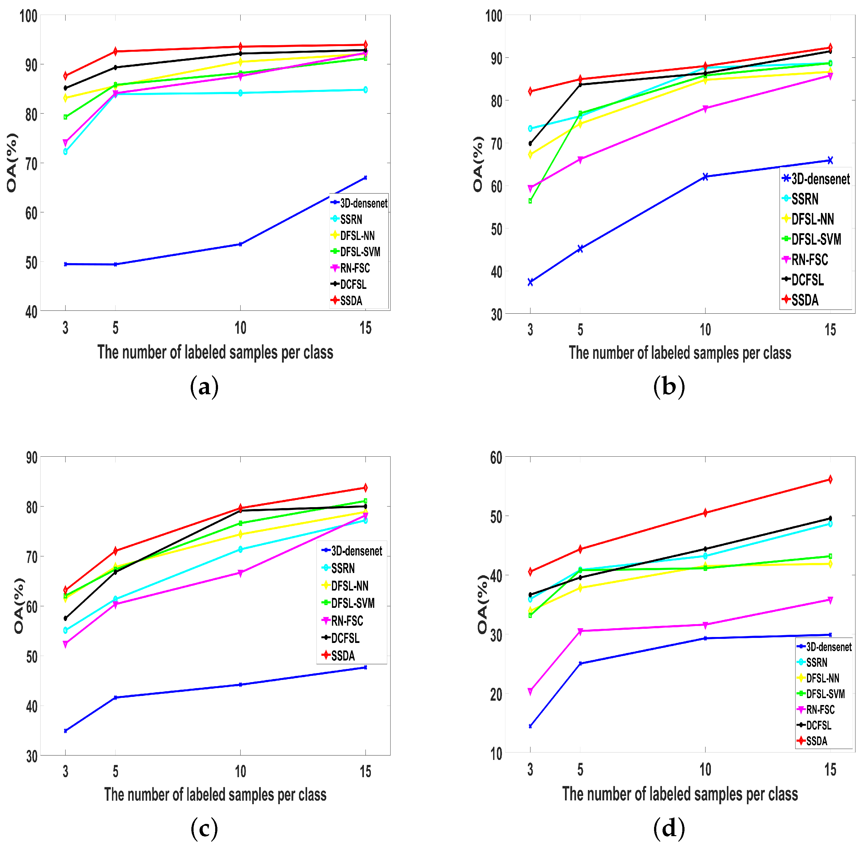
To better verify the robustness of our proposed method, we performed extensive comparative experiments among 3D-DenseNet, SSRN, DFSL + NN, DFSL + SVM, RN-FSC, DCFSL, and our SSDA on the different number of labeled samples per class. We set the number of samples of each class as 3, 5, 10, and 15 on four HSI datasets, respectively. As shown in Figure 14, with the increase of the number of labeled sample, the OA of different algorithms has been improved. In particular, our proposed SSDA also achieves best classification performance among the compared methods. This indicates that our method has stronger robustness than other methods.

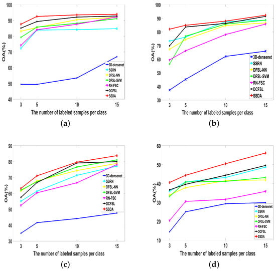
Figure 14. The OA of different methods for different number of labeled samples on Salinas, UP, IP, Huoshaoyun datasets. (a) Salinas; (b) UP; (c) IP; (d) Huoshaoyun.

5.2. Computational Time Comparison

The above experimental results prove that the SSDA obtains higher classification accuracy than state-of-the-art methods on few-shot samples. However, a superior classification method should balance accuracy and efficiency properly. In this part, we show the training time and test time of different methods and the minimum time is shown in bold (Table 11). The computer was equipped with a 2.5 GHZ Intel Xeon CPU, 128 GB, and a Nvidia GeForce GTX 2080 Ti GPU.

Table 11. Computational time (second) on each dataset with different methods.

Datasets	Time	3D-DenseNet	SSRN	DFSL + NN	DFSL + SVM	RN-FSC	DCFSL	SSDA
UP	Train	53.86	688.78	525.27	496.29	548.85	2155.09	1855.86
	Test	6.23	5.21	4.35	4.13	42.58	7.24	8.14
Salinas	Train	63.03	812.15	693.15	1011.73	304.29	2016.29	1207.28
	Test	8.36	4.16	4.39	5.37	34.57	23.93	18.40
IP	Train	62.35	553.36	331.54	527.77	617.89	1805.30	985.39
	Test	1.5	1.68	2.14	3.69	17.21	6.39	11.09
Huoshaoyun	Train	130,097.54	184.59	674.54	423.81	305.26	1171.28	773.54
	Test	8404.65	27.74	2.17	3.93	33.68	2.31	20.46

It has been found that although 3D-DenseNet and DFSL + NN require the least training time and the testing time separately (Table 11); our proposed SSDA achieves the best classification performance (Table 6, Table 7, Table 8 and Table 9). Meanwhile, on the large scale Salinas and Huoshaoyun datasets, our SSDA requires much less training time and testing time than state-of-the-art DCFSL methods. These results indicate that our SSDA can achieve excellent accuracy on HSI few-shot classification with a comparable time.

6. Conclusions

In this article, to improve the HSI few-shot classification accuracy, we propose a novel spectral-spatial domain attention network (SSDA), which includes a spectral-spatial module, a domain attention module, and a multiple loss module. The spectral-spatial module can extract discriminative and domain invariance spectral-spatial features. The domain attention module is designed to further enhance useful features and suppress useless features. The multiple loss module can minimize the difference of source domain and target domain, which can alleviate the domain adaptation issue. Extensive experimental results indicate that the proposed SSDA achieves higher classification accuracy than state-of-the-art methods with few-shot samples on four HSI datasets. However, the complex model results in a slightly high computational complexity. In the future, we will design a more lightweight model structure for fast and high-precision classification.

References

- Landgrebe, D. Hyperspectral image data analysis. IEEE Signal Process. Mag. 2002, 19, 17–28. [Google Scholar] [CrossRef]
- Chen, Y.; Lin, Z.; Zhao, X.; Wang, G.; Gu, Y. Deep learning-based classification of hyperspectral data. IEEE J. Sel. Top. Appl. Earth Obs. Remote Sens. 2014, 7, 2094–2107. [Google Scholar] [CrossRef]
- Zhang, T.; Liu, F. Application of hyperspectral remote sensing in mineral identification and mapping. In Proceedings of the 2012 2nd International Conference on Computer Science and Network Technology, Changchun, China, 29–31 December 2012; pp. 103–106. [Google Scholar] [CrossRef]
- Daukantas, P. Hyperspectral imaging meets biomedicine. Opt. Photonics News 2020, 31, 32–39. [Google Scholar] [CrossRef]
- Nanni, L.; Ghidoni, S.; Brahnam, S. Handcrafted vs. non-handcrafted features for computer vision classification. Pattern Recognit. 2017, 71, 158–172. [Google Scholar] [CrossRef]
- Xue, F.; Tan, F.; Ye, Z.; Chen, J.; Wei, Y. Spectral-Spatial Classification of Hyperspectral Image Using Improved Functional Principal Component Analysis. IEEE Geosci. Remote Sens. Lett. 2022, 19, 5507105. [Google Scholar] [CrossRef]
- Hou, Q.; Wang, Y.; Jing, L.; Chen, H. Linear Discriminant Analysis Based on Kernel-Based Possibilistic C-Means for Hyperspectral Images. IEEE Geosci. Remote Sens. Lett. 2019, 16, 1259–1263. [Google Scholar] [CrossRef]
- Zhang, Y.; Liu, K.; Dong, Y.; Wu, K.; Hu, X. Semisupervised Classification Based on SLIC Segmentation for Hyperspectral Image. IEEE Geosci. Remote Sens. Lett. 2020, 17, 1440–1444. [Google Scholar] [CrossRef]
- Munmun Baisantry, A.K.S.; Shukla, D.P. Selection of shape-preserving, discriminative bands using supervised functional principal component analysis. Int. J. Remote Sens. 2022, 43, 3868–3889. [Google Scholar] [CrossRef]
- Pal, M. Ensemble of support vector machines for land cover classification. Int. J. Remote Sens. 2008, 29, 3043–3049. [Google Scholar] [CrossRef]
- Samaniego, L.; Bárdossy, A.; Schulz, K. Supervised classification of remotely sensed imagery using a modified k-NN technique. IEEE Trans. Geosci. Remote Sens. 2008, 46, 2112–2125. [Google Scholar] [CrossRef]
- Ren, Y.; Zhang, Y.; Wei, W.; Lei, L. A spectral-spatial hyperspectral data classification approach using random forest with label constraints. In Proceedings of the IEEE Workshop on Electronics, Hangzhou, China, 9–11 June 2014. [Google Scholar]
- Bortiew, A.; Patra, S.; Bruzzone, L. Active Learning for Hyperspectral Image Classification Using Kernel Sparse Representation Classifiers. IEEE Geosci. Remote Sens. Lett. 2023, 20, 5503505. [Google Scholar] [CrossRef]
- Zhang, Z.; Liu, D.; Gao, D.; Shi, G. S3Net: Spectral—Spatial—Semantic Network for Hyperspectral Image Classification with the Multiway Attention Mechanism. IEEE Trans. Geosci. Remote Sens. 2022, 60, 5505317. [Google Scholar] [CrossRef]
- Zhang, Z.; Liu, D.; Gao, D.; Shi, G. A novel spectral-spatial multi-scale network for hyperspectral image classification with the Res2Net block. Int. J. Remote Sens. 2022, 43, 751–777. [Google Scholar] [CrossRef]
- Hao, S.; Wang, W.; Salzmann, M. Geometry-Aware Deep Recurrent Neural Networks for Hyperspectral Image Classification. IEEE Trans. Geosci. Remote Sens. 2021, 59, 2448–2460. [Google Scholar] [CrossRef]
- Ghaderizadeh, S.; Abbasi-Moghadam, D.; Sharifi, A.; Zhao, N.; Tariq, A. Hyperspectral Image Classification Using a Hybrid 3D-2D Convolutional Neural Networks. IEEE J. Sel. Top. Appl. Earth Obs. Remote Sens. 2021, 14, 7570–7588. [Google Scholar] [CrossRef]
- Liu, Q.; Xiao, L.; Yang, J.; Chan, J.C.W. Content-Guided Convolutional Neural Network for Hyperspectral Image Classification. IEEE Trans. Geosci. Remote Sens. 2020, 58, 6124–6137. [Google Scholar] [CrossRef]
- Kalchbrenner, N.; Grefenstette, E.; Blunsom, P. A convolutional neural network for modelling sentences. arXiv 2014, arXiv:1404.2188. [Google Scholar]
- Hu, W.; Huang, Y.; Wei, L.; Zhang, F.; Li, H. Deep convolutional neural networks for hyperspectral image classification. J. Sens. 2015, 2015, 258619. [Google Scholar] [CrossRef]
- Li, J.; Zhao, X.; Li, Y.; Du, Q.; Xi, B.; Hu, J. Classification of hyperspectral imagery using a new fully convolutional neural network. IEEE Geosci. Remote Sens. Lett. 2018, 15, 292–296. [Google Scholar] [CrossRef]
- Guo, T.; Wang, R.; Luo, F.; Gong, X.; Zhang, L.; Gao, X. Dual-View Spectral and Global Spatial Feature Fusion Network for Hyperspectral Image Classification. IEEE Trans. Geosci. Remote Sens. 2023, 61, 5512913. [Google Scholar] [CrossRef]
- Song, W.; Dai, Y.; Gao, Z.; Fang, L.; Zhang, Y. Hashing-Based Deep Metric Learning for the Classification of Hyperspectral and LiDAR Data. IEEE Trans. Geosci. Remote Sens. 2023, 61, 5704513. [Google Scholar] [CrossRef]
- Zhou, H.; Luo, F.; Zhuang, H.; Weng, Z.; Gong, X.; Lin, Z. Attention Multihop Graph and Multiscale Convolutional Fusion Network for Hyperspectral Image Classification. IEEE Trans. Geosci. Remote Sens. 2023, 61, 5508614. [Google Scholar] [CrossRef]
- Duan, Y.; Luo, F.; Fu, M.; Niu, Y.; Gong, X. Classification via Structure-Preserved Hypergraph Convolution Network for Hyperspectral Image. IEEE Trans. Geosci. Remote Sens. 2023, 61, 5507113. [Google Scholar] [CrossRef]
- Paoletti, M.E.; Haut, J.M.; Pereira, N.S.; Plaza, J.; Plaza, A. Ghostnet for Hyperspectral Image Classification. IEEE Trans. Geosci. Remote Sens. 2021, 59, 10378–10393. [Google Scholar] [CrossRef]
- Roy, S.K.; Mondal, R.; Paoletti, M.E.; Haut, J.M.; Plaza, A. Morphological Convolutional Neural Networks for Hyperspectral Image Classification. IEEE J. Sel. Top. Appl. Earth Obs. Remote Sens. 2021, 14, 8689–8702. [Google Scholar] [CrossRef]
- Safari, K.; Prasad, S.; Labate, D. A Multiscale Deep Learning Approach for High-Resolution Hyperspectral Image Classification. IEEE Geosci. Remote Sens. Lett. 2021, 18, 167–171. [Google Scholar] [CrossRef]
- Chen, Y.; Zhao, X.; Jia, X. Spectral–spatial classification of hyperspectral data based on deep belief network. IEEE J. Sel. Top. Appl. Earth Obs. Remote Sens. 2015, 8, 2381–2392. [Google Scholar] [CrossRef]
- Mei, S.; Ji, J.; Geng, Y.; Zhang, Z.; Li, X.; Du, Q. Unsupervised Spatial—Spectral Feature Learning by 3D Convolutional Autoencoder for Hyperspectral Classification. IEEE Trans. Geosci. Remote Sens. 2019, 57, 6808–6820. [Google Scholar] [CrossRef]
- Mou, L.; Ghamisi, P.; Zhu, X.X. Unsupervised spectral—Spatial feature learning via deep residual Conv–Deconv network for hyperspectral image classification. IEEE Trans. Geosci. Remote Sens. 2017, 56, 391–406. [Google Scholar] [CrossRef]
- Ma, N.; Peng, Y.; Wang, S.; Leong, P.H. An unsupervised deep hyperspectral anomaly detector. Sensors 2018, 18, 693. [Google Scholar] [CrossRef]
- Tan, K.; Hu, J.; Li, J.; Du, P. A novel semi-supervised hyperspectral image classification approach based on spatial neighborhood information and classifier combination. ISPRS J. Photogramm. Remote Sens. 2015, 105, 19–29. [Google Scholar] [CrossRef]
- Wu, Y.; Mu, G.; Qin, C.; Miao, Q.; Ma, W.; Zhang, X. Semi-supervised hyperspectral image classification via spatial-regulated self-training. Remote Sens. 2020, 12, 159. [Google Scholar] [CrossRef]
- Xie, F.; Hu, D.; Li, F.; Yang, J.; Liu, D. Semi-Supervised Classification for Hyperspectral Images Based on Multiple Classifiers and Relaxation Strategy. ISPRS Int. J.-Geo-Inf. 2018, 7, 284. [Google Scholar] [CrossRef]
- Chen, H.; Ye, M.; Lei, L.; Lu, H.; Qian, Y. Semisupervised Dual-Dictionary Learning for Heterogeneous Transfer Learning on Cross-Scene Hyperspectral Images. IEEE J. Sel. Top. Appl. Earth Obs. Remote Sens. 2020, 13, 3164–3178. [Google Scholar] [CrossRef]
- Sung, F.; Yang, Y.; Zhang, L.; Xiang, T.; Torr, P.H.; Hospedales, T.M. Learning to Compare: Relation Network for Few-Shot Learning. In Proceedings of the IEEE Conference on Computer Vision and Pattern Recognition (CVPR), Salt Lake City, UT, USA, 18–23 June 2018. [Google Scholar]
- Qin, Y.; Bruzzone, L.; Li, B.; Ye, Y. Cross-Domain Collaborative Learning via Cluster Canonical Correlation Analysis and Random Walker for Hyperspectral Image Classification. IEEE Trans. Geosci. Remote Sens. 2019, 57, 3952–3966. [Google Scholar] [CrossRef]
- Ravi, S.; Larochelle, H. Optimization as a model for few-shot learning. In Proceedings of the ICLR 2017, Toulon, France, 24–26 April 2016. [Google Scholar]
- Wang, Y.; Yao, Q.; Kwok, J.T.; Ni, L.M. Generalizing from a Few Examples: A Survey on Few-Shot Learning. ACM Comput. Surv. 2020, 53, 1–34. [Google Scholar] [CrossRef]
- Zhang, C.; Yue, J.; Qin, Q. Global Prototypical Network for Few-Shot Hyperspectral Image Classification. IEEE J. Sel. Top. Appl. Earth Obs. Remote Sens. 2020, 13, 4748–4759. [Google Scholar] [CrossRef]
- Liu, B.; Yu, X.; Yu, A.; Zhang, P.; Wan, G.; Wang, R. Deep few-shot learning for hyperspectral image classification. IEEE Trans. Geosci. Remote Sens. 2018, 57, 2290–2304. [Google Scholar] [CrossRef]
- Gao, K.; Liu, B.; Yu, X.; Qin, J.; Zhang, P.; Tan, X. Deep relation network for hyperspectral image few-shot classification. Remote Sens. 2020, 12, 923. [Google Scholar] [CrossRef]
- Liang, X.; Zhang, Y.; Zhang, J. Attention Multisource Fusion-Based Deep Few-Shot Learning for Hyperspectral Image Classification. IEEE J. Sel. Top. Appl. Earth Obs. Remote Sens. 2021, 14, 8773–8788. [Google Scholar] [CrossRef]
- Zuo, X.; Yu, X.; Liu, B.; Zhang, P.; Tan, X. FSL-EGNN: Edge-Labeling Graph Neural Network for Hyperspectral Image Few-Shot Classification. IEEE Trans. Geosci. Remote Sens. 2022, 60, 5526518. [Google Scholar] [CrossRef]
- Vilalta, R.; Drissi, Y. A perspective view and survey of meta-learning. Artif. Intell. Rev. 2002, 18, 77–95. [Google Scholar] [CrossRef]
- Ying, X.; Wang, L.; Wang, Y.; Sheng, W.; An, W.; Guo, Y. Deformable 3d convolution for video super-resolution. IEEE Signal Process. Lett. 2020, 27, 1500–1504. [Google Scholar] [CrossRef]
- Dai, J.; Qi, H.; Xiong, Y.; Li, Y.; Zhang, G.; Hu, H.; Wei, Y. Deformable convolutional networks. In Proceedings of the IEEE International Conference on Computer Vision, Venice, Italy, 22–29 October 2017; pp. 764–773. [Google Scholar]
- Mou, L.; Zhu, X.X. Learning to Pay Attention on Spectral Domain: A Spectral Attention Module-Based Convolutional Network for Hyperspectral Image Classification. IEEE Trans. Geosci. Remote Sens. 2020, 58, 110–122. [Google Scholar] [CrossRef]
- Yokoya, N.; Iwasaki, A. Airborne Hyperspectral Data over Chikusei; Technical Report SAL-2016-05-27; Space Application Laboratory, University of Tokyo: Tokyo, Japan, 2016. [Google Scholar]
- Zhang, C.; Li, G.; Du, S.; Tan, W.; Gao, F. Three-dimensional densely connected convolutional network for hyperspectral remote sensing image classification. J. Appl. Remote Sens. 2019, 13, 016519. [Google Scholar] [CrossRef]
- Zhong, Z.; Li, J.; Luo, Z.; Chapman, M. Spectral–spatial residual network for hyperspectral image classification: A 3-D deep learning framework. IEEE Trans. Geosci. Remote Sens. 2017, 56, 847–858. [Google Scholar] [CrossRef]
- Li, Z.; Liu, M.; Chen, Y.; Xu, Y.; Li, W.; Du, Q. Deep cross-domain few-shot learning for hyperspectral image classification. IEEE Trans. Geosci. Remote Sens. 2021, 60, 5501618. [Google Scholar] [CrossRef]
Disclaimer/Publisher’s Note: The statements, opinions and data contained in all publications are solely those of the individual author(s) and contributor(s) and not of MDPI and/or the editor(s). MDPI and/or the editor(s) disclaim responsibility for any injury to people or property resulting from any ideas, methods, instructions or products referred to in the content. |
© 2024 by the authors. Licensee MDPI, Basel, Switzerland. This article is an open access article distributed under the terms and conditions of the Creative Commons Attribution (CC BY) license (https://creativecommons.org/licenses/by/4.0/).