Beam-Space Post-Doppler Reduced-Dimension STAP Based on Sparse Bayesian Learning

Abstract

The space–time adaptive processing (STAP) technique can effectively suppress the ground clutter faced by the airborne radar during its downward-looking operation and thus can significantly improve the detection performance of moving targets. However, the optimal STAP requires a large number of independent identically distributed (i.i.d) samples to accurately estimate the clutter plus noise covariance matrix (CNCM), which limits its application in practice. In this paper, we fully consider the heterogeneity of clutter in real-world environments and propose a sparse Bayesian learning-based reduced-dimension STAP method that achieves suboptimal clutter suppression performance using only a single sample. First, the sparse Bayesian learning (SBL) algorithm is used to estimate the CNCM using a single training sample. Second, a novel angular Doppler channel selection algorithm is proposed with the criterion of maximizing the output signal-to-clutter-noise ratio (SCNR). Finally, the reduced-dimension STAP filter is constructed using the selected channels. Simulation results show that the proposed algorithm can achieve suboptimal clutter suppression performance in extremely heterogeneous clutter environments where only one training sample can be used.

1. Introduction

Airborne radar is highly valued by many countries in the world because of its strong maneuverability and longer direct viewing distance than ground radar. However, due to the influence of ground clutter, the moving target detection performance of airborne radar will be seriously degraded when looking down. The ground clutter is not only strong but also has different speeds relative to the aircraft in different directions, which greatly broadens the clutter spectrum. How to suppress ground clutter is the key problem to be solved in airborne radar systems. Space–time adaptive processing (STAP) [1] technology has been widely used by many researchers because of its excellent ground clutter suppression performance. Traditional STAP algorithms need to use target-free samples adjacent to the cell under test (CUT) to obtain an estimate of the clutter plus noise covariance matrix (CNCM). According to the Reed–Mallett–Brennan (RMB) criterion [2], the output signal-to-clutter-noise ratio (SINR) loss after processing by the STAP algorithm is less than 3 dB only if the number of training samples used is more than two times the number of degrees of freedom (DOFs) of the system. Unfortunately, it is difficult in reality to provide such a large number of i.i.d samples for airborne radar since ground clutter is often heterogeneous due to external non-ideal factors. Therefore, the study of STAP algorithms with few samples and high performance is very important for practical applications.

In the decades since the STAP algorithm was first proposed, numerous researchers have proposed many methods that can reduce the sample requirements of the STAP to some extent. Klemm proposed an auxiliary channel method (ACP) [3], which can effectively reduce the number of i.i.d samples required for STAP. Under ideal conditions, ACP can achieve near-optimal performance, but when non-ideal factors (such as internal clutter motion and array amplitude and phase errors) are present, the performance loss can be significant. Dipietro proposed the extended factor approach (EFA) [4], which uses all spatial domain channels for adaptive processing after Doppler filtering. As a result, EFA is robust to non-ideal factors in the spatial domain. However, when the airborne radar system has a large number of spatial DOFs, EFA still requires many training samples. Wang proposed a joint domain localized processing algorithm (JDL) [5] for space–time adaptive processing by selecting multiple channels adjacent to the channels to be detected in the angular Doppler plane. Compared with EFA, this method has the advantage of further reducing the training sample and lowering the computational complexity and the disadvantage of being more affected by non-ideal factors. In the study of STAP techniques based on spatial–temporal spectral sparsity, the literature [6,7,8,9,10,11,12] utilizes several training samples without target signals to reconstruct the spatial–temporal amplitude spectrum of the clutter and estimate the CNCM. This type of method has the advantage of estimating the clutter covariance matrix relatively accurately using only 4–6 i.i.d training samples, but it also suffers from high computational complexity and inevitable off-grid problems.

In this paper, an RD STAP method based on the sparse Bayesian algorithm is proposed, which has the advantages of requiring fewer samples and suitable clutter suppression performance. In the traditional RD STAP algorithm, we found the following phenomenon, i.e., when the number of samples is insufficient, the output SINR obtained using the RD matrix to process the estimated CNCM followed by adaptive processing is larger than that obtained by directly using the estimated CNCM for adaptive processing. Inspired by this, we consider estimating an inaccurate CNCM using only a single sample in the extremely heterogeneous clutter environment and then selecting the optimal RD channel to make the output SINR satisfy the target detection requirements. In our proposed algorithm, the CNCM is first estimated using the SBL algorithm when only a single sample is available. Although this estimated CNCM cannot be used directly for adaptive processing, it can be used to construct RD transformation matrices. Second, the proposed channel selection algorithm is utilized to select the optimal RD channel in the angular Doppler plane with the criterion of maximizing the output SINR. Finally, the selected channels and estimated CNCM are used to construct the RD STAP filter. The main contributions of this paper are as follows:

• A novel RD STAP method based on the SBL algorithm is proposed, which has suboptimal clutter suppression performance in extremely heterogeneous clutter environments with only one training sample available.
• A novel angular Doppler domain RD channel selection algorithm is proposed, which maximizes the output SINR as a criterion for selecting auxiliary channels. In general, suboptimal clutter suppression performance can be achieved by selecting 3–8 auxiliary channels using the proposed algorithm.

In order to more clearly show the superiority of the proposed algorithm in sample demand, Table 1 lists the minimum number of samples required by several related algorithms to achieve suboptimal performance. In Table 1, $M$ refers to the number of pulses and $N$ refers to the number of elements.

Table 1. Training samples required by several related algorithms.

Algorithm	Required Samples
EFA [4]	6N
JDL(3*3) [5]	18
SBL-STAP [9]	6
Proposed method	1

The remainder of this paper is organized according to the structure below. In Section 2, we briefly review the STAP model and processors based on the GSC architecture. In Section 3, we derive the processing flow of the proposed algorithm in detail. In Section 4, we perform extensive simulation experiments to illustrate the effectiveness of the proposed algorithm. Finally, in Section 5, we summarize some useful conclusions.

Notation: In this paper, the symbol $\otimes$ denotes the Kronecker product. The symbol ${‖·‖}_F$ and ${‖·‖}_0$ are used to represent the Frobenius $\left({\mathcal{l}}_F\right)$ norms and ${\mathcal{l}}_0$ pseudo-norms, respectively. Scalars are italicized, and lowercase bold and uppercase bold denote vectors and matrices, respectively. The operators ${\left(·\right)}^T$ and ${\left(·\right)}^H$ denote transpose and conjugate transpose, respectively. The operation of finding the expectation of a random variable $v$ is denoted by $E\left(v\right)$. The symbol $A\in B$ presents set $A$ belongs to set $B$. The empty set is represented by the symbol $\varnothing$.

2. STAP Model and GSC form Processor

2.1. STAP Model

The system considered is a pulse Doppler radar installed on an airborne platform. The antenna of this radar is a uniform line array (ULA) containing $N$ array elements with a spacing $d$ equal to half of the operating wavelength $\lambda$ of the system. The airborne platform is flying at an altitude of $h$ and a speed of $v$. The radar transmits a coherent burst of pulses at a fixed pulse repetition frequency (PRF) $f_r=1/T_r$, where $T_r$ refers to the pulse repetition time (PRT). A total of $M$ pulses are transmitted during the coherent processing interval (CPI), so the length of the coherent processing time is $M{T}_r$. The geometric model of the airborne radar is shown in Figure 1a. Each PRT needs to be sampled $L$ times to cover the distance interval, and $LMN$ complex baseband samples are obtained after matched filtering the returns from each pulse within a CPI, which is referred to as radar datacube, shown in Figure 1b.

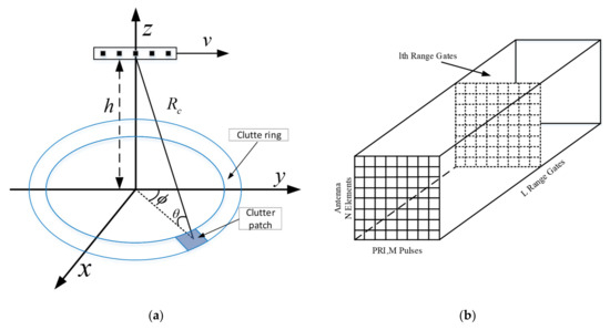
Figure 1. Airborne radar geometric configuration and datacube. (a) Airborne radar downward-looking working model; (b) the radar datacube.

According to the clutter model proposed by Ward [1], the normalized spatial and normalized Doppler frequency of the $i\text{-}th$ clutter patch can be expressed as

$$f_{d,i}=\frac{2v}{\lambda f_r}\cos \left({\theta }_i\right)\cos \left({\phi }_i\right)$$

(1)

$$f_{s,i}=\frac{d}{\lambda }\cos \left({\theta }_i\right)\cos \left({\phi }_i\right)$$

(2)

where ${\theta }_i$ and ${\phi }_i$ are the elevation and azimuth angle, respectively. Then, the space–time steering vector can be expressed as

$$s\left(f_{d,i},f_{s,i}\right)=a\left(f_{d,i}\right)\otimes b\left(f_{s,i}\right)$$

(3)

$$a\left(f_{d,i}\right)={\left[1 \exp \left(j2\pi f_{d,i}\right) \cdots \exp \left(j2\pi \left(M-1\right)f_{d,i}\right)\right]}^T$$

(4)

$$b\left(f_{s,i}\right)={\left[1 \exp \left(j2\pi f_{s,i}\right) \cdots \exp \left(j2\pi \left(N-1\right)f_{s,i}\right)\right]}^T$$

(5)

where $a\left(f_{d,i}\right)$ and $b\left(f_{s,i}\right)$ are the time and spatial steering vectors, respectively. Considering the range ambiguity, the space–time snapshot can be expressed as [1]

$$x_l=x_c+x_n={\displaystyle \sum _{a=1}^{Na}{\displaystyle \sum _{i=1}^{N_c}{\alpha }_{a,i}s\left(f_{d,a,i},f_{s,a,i}\right)}}+x_n$$

(6)

where ${\alpha }_{a,i}$ represents the random complex amplitude of the $i\text{-}th$ clutter patch of $a\text{-}th$ ambiguous range. $x_n$ is modeled as zero mean Gaussian white noise. Assuming that the clutter patches are independent of each other, the ideal CNCM can be calculated as

$$R_{c+n}=\mathrm{\Phi }\mathrm{\Gamma }{\mathrm{\Phi }}^H+{\sigma }^2{I}_{MN}=R_c+{\sigma }^2{I}_{MN}$$

(7)

where $R_c$ represents the clutter covariance matrix, ${\sigma }^2$ represents the noise power, $\mathrm{\Phi }\in C^{MN\times N_c}$ denotes the matrix consisting of the space–time steering vectors of each clutter patch, $\mathrm{\Gamma }\in C^{N_c\times N_c}$ is a diagonal matrix with the main diagonal elements being the power of each clutter patch. Assuming that $v_t$ is the space–time steering vector of the target, the optimal STAP filtering weight can be obtained by solving the following optimization problem [13]:

$$\begin{array}{cc}\min & W_{opt}^H{R}_{c+n}{W}_{opt}\\ s.t.& W_{opt}^H{v}_t=1\end{array}$$

(8)

and the optimal weight is expressed as

$$W_{opt}=\frac{R_{c+n}^{-1}{v}_t}{v_t^H{R}_{c+n}^{-1}{v}_t}$$

(9)

In the traditional SR STAP algorithm, we discretized the normalized space–time plane uniformly to $K=N_s{N}_d$ points, where $N_s\gg N$ is the number of spatial channels and $N_d\gg M$ is the number of Doppler channels. Then, the SR signal model with single measurement vectors (SMV) is expressed as [14]

$$x=Dw+\epsilon$$

(10)

where $x$ represents the measurement vector and $D$ is the space–time overcomplete dictionary obtained by discretizing the space–time plane. $\epsilon$ represents the additive zero mean Gaussian white noise vector. $w$ is a sparse coefficient vector, which is also the parameter to be solved. The sparse coefficient solution problem in Equation (10) can be approximated as the following convex optimization problem [15]:

$$\begin{array}{cc}\underset{w}{\min }& {‖w‖}_1\\ s.t.& {‖x-Dw‖}_2\le \rho \end{array}$$

(11)

where $\rho$ denotes the fitting error tolerance.

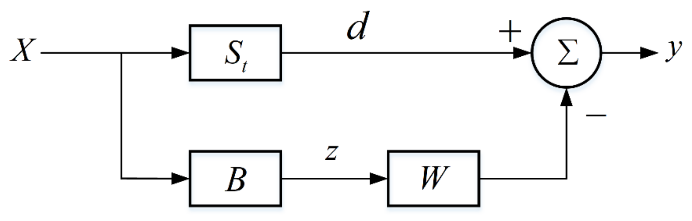
2.2. GSC form Processor

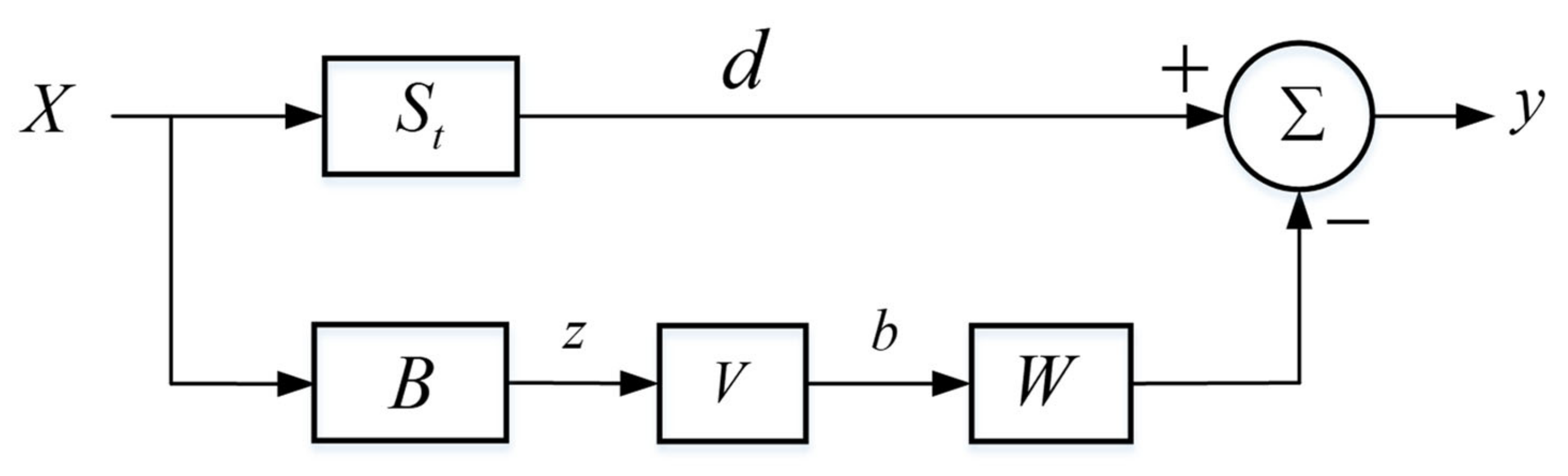
As shown in Figure 2, the GSC structure processer is divided into upper and lower branches [16,17]. The upper branch is the main channel containing the target and clutter component, and the lower branch is the auxiliary channel containing only the clutter component. The GSC processor can improve the SINR in the main channel by utilizing the clutter in the auxiliary channel to cancel the clutter in the main channel. The space–time steering vector of the main channel can be expressed as

$$S_t\left(f_{d,t},f_{s,t}\right)=a\left(f_{d,t}\right)\otimes b\left(f_{s,t}\right)$$

(12)

where $f_{d,t}$ and $f_{s,t}$ denote the normalized spatial and normalized Doppler frequency, respectively. And $a\left(f_{d,t}\right)$ and $b\left(f_{s,t}\right)$ are the time and spatial steering vector, respectively. The matrix $B$ of the lower branch represents the blocking matrix, which consists of the angular Doppler channel other than the main channel. On the one hand, there is no dimensionality reduction in the STAP processing when $B$ contains all angular Doppler channels other than the main channel. On the other hand, different subsets of all angular Doppler channels other than the main channel can be selected to form different RD STAP algorithms.

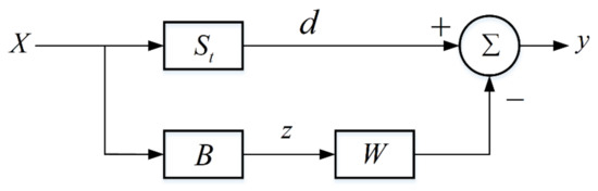
Figure 2. GSC form processor.

The GSC processor transforms the space–time adaptive processing detection structure into a standard Wiener filter. As shown in Figure 2, the output of the GSC filter without reduced dimension can be expressed as

$$y=d-W^{H}z$$

(13)

where $d$ is the output of the upper branch and $z\in C^{\left(NM-1\right)\times 1}$ is the clutter vector that does not contain the target, given by

$$d=S_t^{H}X$$

(14)

$$z=B^{H}X$$

(15)

where $B\in C^{NM\times \left(NM-1\right)}$ is the blocking matrix, which is composed of space–time steer vectors of different angular Doppler channels except the main channel. It is well known that angular Doppler channels are perpendicular to each other. Therefore, we have

$$B^H{S}_t=0\in C^{\left(MN-1\right)\times 1}$$

(16)

The design philosophy of the GSC filter is to minimize the output power, which gives rise to the following optimization problem.

$$\underset{W}{\min }J\left(W\right)=\underset{W}{\min }E\left[{‖y‖}_2^2\right]$$

(17)

The optimal weight vector is calculated as

$$W_{opt}=R_z^{-1}{r}_{zd}$$

(18)

where $R_z$ denotes the CNCM of the lower branch

$$R_z=E\left[z{z}^H\right]$$

(19)

$r_{Zd}$ is the cross-correlation vector between the upper and lower branch outputs.

$$r_{zd}=E\left[z{d}^{*}\right]$$

(20)

3. Proposed Algorithm

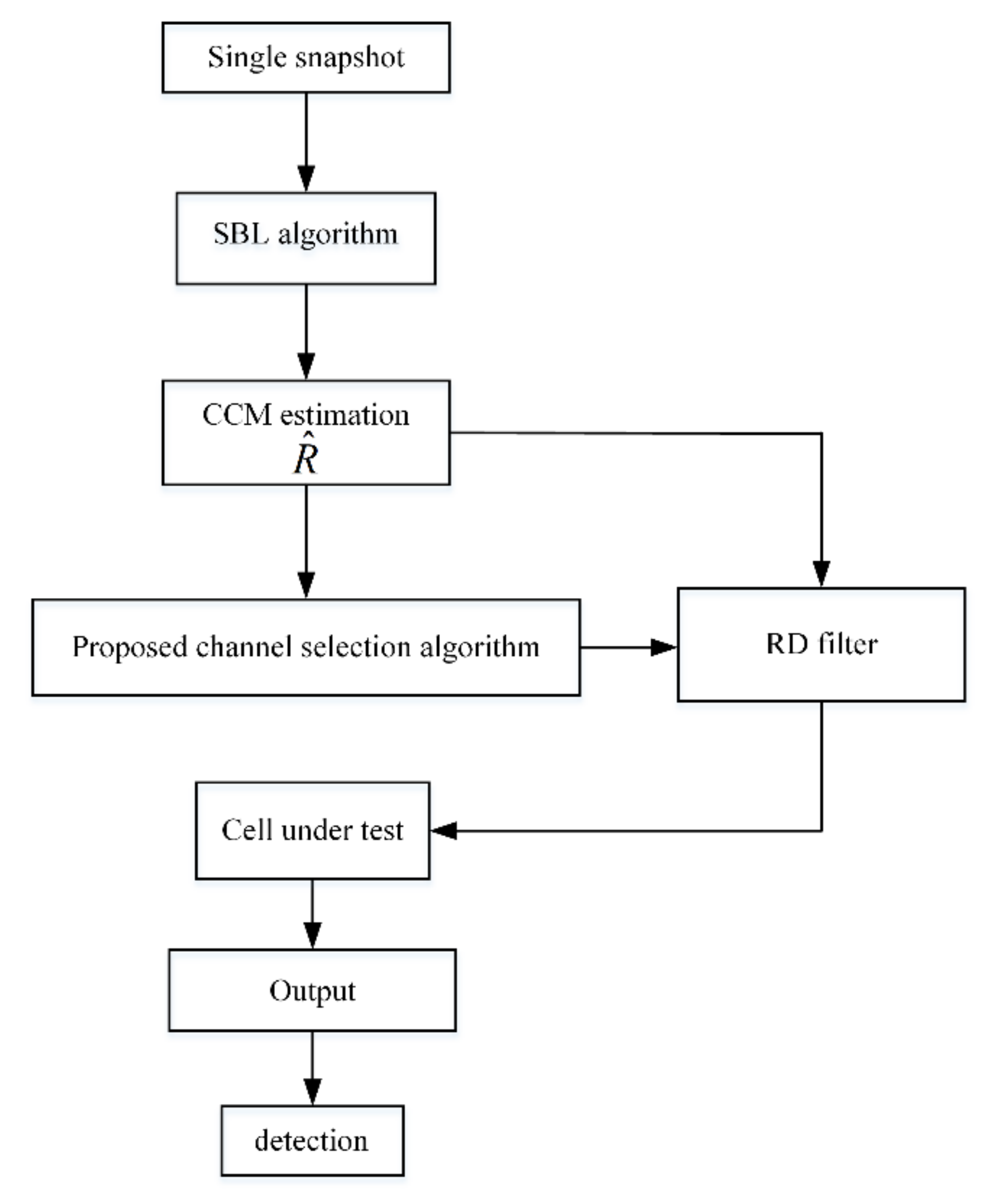
In the proposed algorithm, the CNCM of the cell under test $\widehat{R}$ is first estimated by the SBL algorithm. Then, $\widehat{R}$ and the proposed angular Doppler channel selection algorithm are used to design the RD transformation matrix $T_r$. When $T_r$ is obtained, $T_r$ and $\widehat{R}$ are uesd to design the RD filter. Finally, the RD filter is used to process the data of the CUT and detect the target. The flowchart of the proposed algorithm is shown in Figure 3.

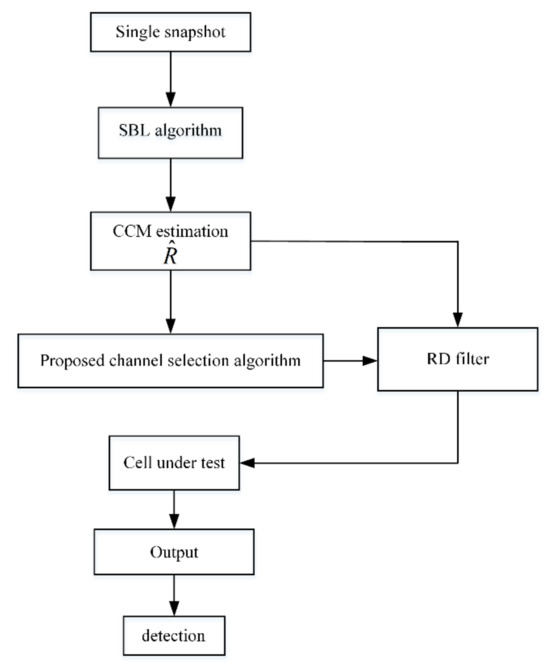
Figure 3. The flowchart of the proposed algorithm.

3.1. CNCM Estimation Method Based on SBL

In this section, we first derive the method for estimating the CNCM using SBL when only a single sample is available and then provide a pseudo-code for computing the covariance matrix. Rewrite the sparse signal model expressed in Equation (10) as follows.

$$x=Dw+\epsilon$$

(21)

where $x\in C^{MN}$ is the measurement data vector, which is the single sample used in the proposed algorithm. $D\in C^{MN\times N_s{N}_d}$ is an overcomplete space–time dictionary obtained by discretizing the normalized space–time plane. $w\in C^{N_s{N}_d\times 1}$ is the sparse coefficient vector to be solved. $\epsilon \in C^{MN\times 1}$ is the noise vector with mean 0 and variance ${\sigma }^2{\mathbf{I}}_{MN}$, and noise power ${\sigma }^2$ is the unknown parameter. Based on the above assumptions, the likelihood probability density function of $x$ has the following form:

$$p\left(\left.x\right|w,{\sigma }^2\right)={\left(2\pi {\sigma }^2\right)}^{-\frac{MN}{2}}\exp \left(-\frac{1}{2{\sigma }^2}{‖x-Dw‖}^2\right)$$

(22)

To ensure the sparsity of the model, we assign to each element of $w$ a Gaussian prior with zero mean and ${\alpha }_i^{-1}$ variance. As a result, the joint distribution of each element in $w$ can be expressed as

$$p\left(\left.w\right|\alpha \right)={\displaystyle \prod _{i=1}^{N_s{N}_d}{\left(2\pi \right)}^{-\frac{1}{2}}{\alpha }_i^{\frac{1}{2}}\exp \left(-\frac{{\alpha }_i}{2}{w}_i^2\right)}$$

(23)

where $\alpha ={\left[{\alpha }_1^{-1},{\alpha }_2^{-1},\cdots ,{\alpha }_{N_d{N}_s}^{-1}\right]}^T$ is the hyperparameters vector. According to [18], the suitable priors thereover are Gamma distributions for $\alpha$ and ${\sigma }^2$. As a result, the joint probability density function of the elements in vector $\alpha$ can be expressed as

$$p\left(\alpha \right)={\displaystyle \prod _{i=1}^{N_s{N}_d}Gamma\left(\left.{\alpha }_i\right|a,b\right)}$$

(24)

$$p\left({\sigma }^{-2}\right)=Gamma\left(\left.{\sigma }^{-2}\right|c,d\right)$$

(25)

where

$$Gamma\left(\left.\alpha \right|a,b\right)=\mathrm{\Gamma }{\left(a\right)}^{-1}{b}^a{\alpha }^{a-1}{e}^{-b\alpha }$$

(26)

with $\mathrm{\Gamma }\left(a\right)={\displaystyle {\int }_0^{\infty }{t}^{a-1}{e}^{-t}}dt$. To make these priors non-informative [18], we might fix their parameters to small values: e.g., $a=b=c=d={10}^{-6}$. Then, calculating the estimates of each parameter based on the given data can be accomplished by calculating the posterior probability density function as follows:

$$p\left(\left.w,\alpha ,{\sigma }^2\right|x\right)=\frac{p\left(\left.x\right|w,\alpha ,{\sigma }^2\right)p\left(w,\alpha ,{\sigma }^2\right)}{p\left(x\right)}$$

(27)

To simplify the calculation, this posterior is written in another equivalent form:

$$p\left(\left.w,\alpha ,{\sigma }^2\right|x\right)=p\left(\left.w\right|x,\alpha ,{\sigma }^2\right)p\left(\left.\alpha ,{\sigma }^2\right|x\right)$$

(28)

According to the famous Bayes’ theorem, the posterior distribution over the $w$ is thus given by [18]

$$\begin{array}{cc}p\left(\left.w\right|x,\alpha ,{\sigma }^2\right)\hfill & =\frac{p\left(\left.x\right|w,{\sigma }^2\right)p\left(\left.w\right|\alpha \right)}{p\left(\left.x\right|\alpha ,{\sigma }^2\right)}\hfill \\ & ={\left(2\pi \right)}^{-\frac{N_s{N}_d}{2}}{\left|\mathrm{\Sigma }\right|}^{-\frac{1}{2}}\exp \left(-\frac{1}{2}{\left(w-\mu \right)}^T{\mathrm{\Sigma }}^{-1}\left(w-\mu \right)\right)\hfill \end{array}$$

(29)

Therefore, the posterior covariance and mean are expressed respectively as [19,20]

$$\mathrm{\Sigma }={\left({\sigma }^{-2}{D}^{H}D+\mathrm{\Lambda }\right)}^{-1}$$

(30)

$$\mu ={\sigma }^{-2}\mathrm{\Sigma }{D}^{H}x$$

(31)

where $\mathrm{\Lambda }=diag\left(\left[{\alpha }_1,{\alpha }_2,\cdots ,{\alpha }_{N_s{N}_d}\right]\right)$.

Next, the expectation maximization (EM) [18] algorithm is used to update the hyperparameters $\alpha$ and ${\sigma }^2$. First, calculate the updated formula for the hyperparameter $\alpha$. Ignoring the terms in the logarithm that are not relevant to $\alpha$, we can obtain the following expectation:

$$E_{\left.w\right|t,\alpha ,\beta }\left(\log \left(p\left(\left.w\right|\alpha \right)p\left(\alpha \right)\right)\right)$$

(32)

We maximize this expectation to obtain an iterative update formula for $\alpha$. By differentiating this expectation in Equation (32) and making the derivative equal to 0, we obtain the following iterative updating equation:

$${\left({\alpha }_i\right)}^{new}=\frac{1}{E_{\left.w\right|t,\alpha ,\beta }\left(w_i^2\right)}=\frac{1}{{\mathrm{\Sigma }}_{i,i}+{\mu }_i^2}$$

(33)

By following the same steps as before, we can obtain the following expectation associated only with ${\sigma }^{-2}$:

$$E_{\left.w\right|t,\alpha ,\beta }\left(\log \left(p\left(\left.x\right|w,\beta \right)p\left(\beta \right)\right)\right)$$

(34)

By maximizing the expectation in Equation (34), we can obtain an iterative update formula for ${\sigma }^2$:

$${\left({\sigma }^2\right)}^{new}=\frac{E_{\left.w\right|t,\alpha ,\beta }\left({‖x-Dw‖}^2\right)}{N_s{N}_d}=\frac{{‖x-D\mu ‖}^2+trace\left(\mathrm{\Sigma }{D}^{H}D\right)}{N_s{N}_d}$$

(35)

The iterative updates of $\alpha$ and ${\sigma }^2$ does not stop until the preset constraints are satisfied. After the iterative updating of the parameters converges, the CNCM can be calculated as

$$\widehat{R}=D\mathrm{\Pi }{D}^H+{\sigma }^2{I}_{MN}$$

(36)

where $\mathrm{\Pi }=diag\left(\left[{\mu }_1^2,{\mu }_2^2,\cdots ,{\mu }_{N_s{N}_d}^2\right]\right)$.

The pseudo-code for the SBL-based CNCM estimation method is shown in Algorithm 1.

Algorithm 1. CNCM estimation method based on SBL.

Step1: Given the initial values ${\sigma }_0^2=0.01$, ${\alpha }_{0,i}=1,i=1,2,\cdots ,N_s{N}_d$ Step2: Compute the posterior moments  ${\mathrm{\Sigma }}_{k+1}={\left({\sigma }_k^{-2}{D}^{H}D+{\mathrm{\Lambda }}_k\right)}^{-1}$  ${\mu }_{k+1}={\sigma }_k^{-2}{\mathrm{\Sigma }}_{k+1}{D}^{H}x$ Step3: Update the $\alpha$ and ${\sigma }^2$ using the EM rule  ${\alpha }_{k+1,i}=\frac{1}{{\mathrm{\Sigma }}_{k+1,i,i}+{\mu }_{k+1,i}^2}$  ${\sigma }_{k+1}^2=\frac{{‖x-D{\mu }_{k+1}‖}^2+trace\left({\mathrm{\Sigma }}_{k+1}{D}^{H}D\right)}{N_s{N}_d}$ Step4: Continue Step 2 and 3 until convergence Step5: Assuming $\widehat{w}={\mu }_{k+1}$ Step6: Compute the CNCM by  $\widehat{R}=D\widehat{w}{\widehat{w}}^H{D}^H+{\sigma }_{k+1}^2{I}_{MN}$

3.2. Channel Selection Algorithm Based on SINR Maximum Criterion

As shown in Figure 4, the matrix $V$ in the lower branch denotes the selection matrix, which consists of some columns of the unit matrix. If $K$ channels are selected as auxiliary channels, then the selection matrix $V$ will consist of the $K$ columns of the unit matrix and the DOF of the filter is reduced from $\left(NM-1\right)$ to $K$. In RD STAP, the RD observation data vector is formed using the selection matrix $V\in C^{(NM-1)\times K}$:

$$b=V^{H}z\in C^{K\times 1}$$

(37)

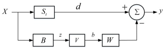
Figure 4. Reduced-dimension GSC form processor.

The corresponding $K\times K$ RD CNCM is shown below.

$$R_b=V^H{R}_{z}V\in C^{K\times K}$$

(38)

Now, we need to specify how to select the optimal auxiliary channel. We propose an iterative algorithm for selecting the auxiliary channel using the maximum output SINR as a criterion. When selecting the first channel, we need to choose the one that maximizes the output SINR from the $J=\left(MN-1\right)$ candidates. When we choose the $j\text{-}th$ channel as the first auxiliary channel, the selection matrix $V=\left[e_j\right]$ has only one column, where $e_j$ represents the $j\text{-}th$ column of the unit matrix. In this case, the RD matrix can then be expressed as

$$T_r=\left[S_t,BV\right]\in C^{NM\times 2}$$

(39)

Apply the RD matrix to the estimated CNCM $\widehat{R}$ to obtain the localized CNCM ${\widehat{R}}_{Local}$.

$${\widehat{R}}_{Local}=T_r^H\widehat{R}{T}_r\in C^{2\times 2}$$

(40)

According to [21], we have the following relationship:

$${\widehat{R}}_{Local}=\left[\begin{array}{cc}{\sigma }_d^2& {\widehat{r}}_{bd}^H\\ {\widehat{r}}_{bd}& {\widehat{R}}_b\end{array}\right]$$

(41)

Based on the conclusions of Equation (18), the filter weight under the RD GSC structure can be expressed as

$$W={\widehat{R}}_{Local}^{-1}{\widehat{r}}_{bd}$$

(42)

and we have

$$W_T=\left[\begin{array}{c}1\\ -W\end{array}\right]$$

(43)

The output SINR when the $j\text{-}th$ auxiliary channel is selected can be calculated by the following equation:

$$SIN{R}_j=\frac{{\left|W_T^H{S}_T\right|}^2}{W_T^H{\widehat{R}}_{Local}{W}_T},j=1,2,\cdots ,J$$

(44)

The angular Doppler channel that maximizes the output SINR is the first auxiliary channel selected. The problem of finding the maximum output SINR is expressed as follows:

$$m=\underset{j}{\max }\left(SIN{R}_j\right)$$

(45)

Then, the selection matrix $V=\left[e_m\right]$, for the sake of expression, let $v_1=e_m$, this means that the first column of the selection matrix is $e_m$. Then, the selected channel is deleted from the candidate channel, and there are $\left(NM-2\right)$ candidate channels left.

When we select the $k\text{-}th$ auxiliary channel, there are already $\left(k-1\right)$ channels selected and $\left(MN-k-2\right)$ candidate channels left. The selection matrix $V$ can be expressed as

$$V=\left[v_1,\cdots ,v_{k-1},v_k\right]$$

(46)

where $v_1,\cdots ,v_{k-1}$ have been selected in the previous step, and $v_k$ is the channel to be selected. In other words, the selection matrix $V$ in Equation (46) has only one column to be determined, namely $v_k$. In this case, the RD matrix is $T_r\in C^{MN\times \left(k+1\right)}$, and the localized CNCM is ${\widehat{R}}_{Local}\in C^{\left(k+1\right)\times \left(k+1\right)}$. Calculate the output SINR according to Equations (39)–(45) and select the channel with the largest output SINR as $v_k$. In general, selecting 3–5 channels can achieve suboptimal clutter suppression performance.

The pseudo-code of the proposed channel selection algorithm is represented in Algorithm 2. It should be emphasized that the proposed channel selection algorithm is an iterative algorithm. Before use, you can preset the number of channels to be used as the iteration stop condition. For example, if you want the algorithm to stop when $C$ channels are selected, then the $C$ channels selected have the largest output SINR compared to other channel combinations with the same number of channels. Step2 and Step3 in Algorithm 2 are the core iteration steps. Each time Step2 and Step3 are executed, one channel will be selected and the number of candidate channels will be reduced by one.

Algorithm 2. The pseudo-code of the proposed channel selection algorithm.

Step1: Given the initial value:  Estimated covariance matrix $\widehat{R}$  selection matrix $V\in \varnothing$  blocking matrix B contains all candidate auxiliary channels  total number of candidate channels $J=(MN-1)$ Step2: Loop: $j=1,2,\cdots ,J$   $Q=\left[V,e_j\right]$   $T_r=\left[S_t,BQ\right]$   ${\widehat{R}}_{Local}=T_r^H\widehat{R}T$   $W={\widehat{R}}_{Local}^{-1}{\widehat{r}}_{bd}$   $W_T=\left[\begin{array}{c}1\\ -W\end{array}\right]$   $SIN{R}_j=\frac{{\left|W_T^H{S}_T\right|}^2}{W_T^H{\widehat{R}}_{Local}{W}_T}$   $SINR\left(j\right)=SIN{R}_j$  end loop Step3: solve $m=\underset{j}{\max }\left(SINR(j)\right)$  Let $V=\left[V,e_m\right]$, and remove $B{e}_m$ from candidate channel  the number of remaining candidate channels $J=J-1$ Step4: Continue Step2 and Step3 until preset constraints are satisfied. Output: Selection matrix $V$

4. Numerical Simulation

In this section, we will compare the performance of the proposed algorithm with several existing classical algorithms of the same type through simulation experiments. The performance is mainly judged by the output SINR and output SINR loss, and the formulas for calculating these two metrics are provided below [1]:

$$SINR=\frac{{\sigma }^2{\xi }_t{\left|W^H{S}_t\right|}^2}{W^{H}RW}$$

(47)

$$LSINR=\frac{{\sigma }^2}{MN}\frac{{\left|W^H{S}_t\right|}^2}{W^{H}RW}$$

(48)

where $R$, $W$, and ${\xi }_t$ refer to the ideal CNCM, STAP filter weight, and preset signal-to-noise ratio (SNR), respectively.

An airborne phased array radar system is considered in the simulation, and the preset simulation parameters are shown in Table 2. To ensure that the simulations are correct, all the simulation results in the paper are the average of 100 Monte Carlo experiments.

Table 2. List of simulation parameters.

Symbols	Parameters	Value
$\lambda$	wavelength	0.25 m
$d$	element spacing	0.125 m
$v$	velocity	125 m/s
$H$	height	8000 m
$M$	number of pulses	12
$N$	number of elements	12
$f_r$	PRF	2000 Hz
$f_s$	sampling frequency	1 MHz
${\theta }_m$	main lobe elevation angle	0°
${\varphi }_m$	main lobe azimuth angle	90°
${\xi }_c$	CNR	40 dB
${\xi }_t$	SNR	10 dB
$N_s$	Angular discretization	4 N
$N_d$	Doppler discretization	4 M

4.1. Performance Analysis Based on Simulation Data

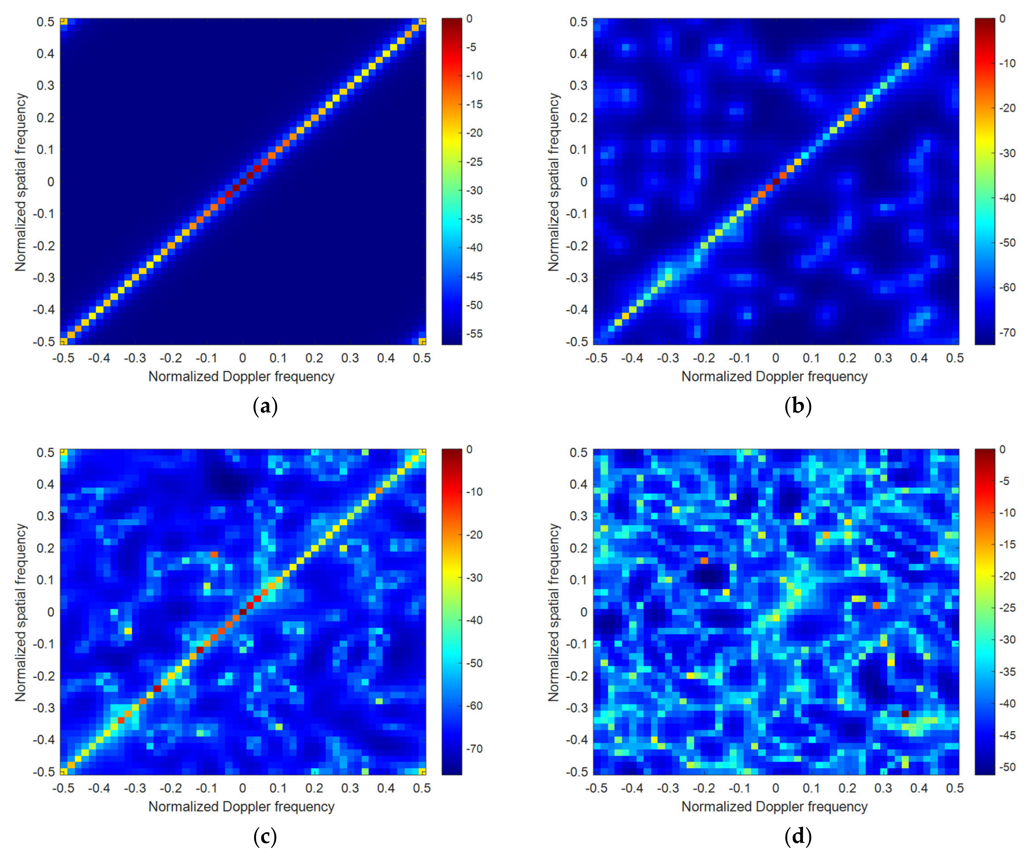
In order to clearly state the simulation results in this section, the intuitive view of the clutter Capon spectrum of the data used in the simulation is given. Figure 5a shows the known ideal Capon spectrum of the CUT. Figure 5b shows the Capon spectrum estimated by the SBL algorithm, with only a single sample available. The value of the color bar in Figure 5 represents the normalized value of the clutter distribution relative to the main lobe on the space–time two-dimensional plane. Figure 5c,d show the clutter Capon spectra obtained using 100 training samples and 10 training samples according to the ML estimation method, respectively. By comparing these four Capon spectra in Figure 5, it can be clearly seen that the accuracy of the Capon spectra estimated by the SBL algorithm is between those estimated by 100 and 10 samples, respectively.

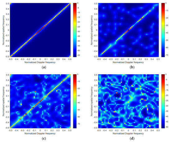
Figure 5. Comparison of estimated clutter Capon spectra. (a) Ideal CNCM; (b) SBL, a single snapshot; (c) ML, 100 snapshots; (d) ML, 10 snapshots.

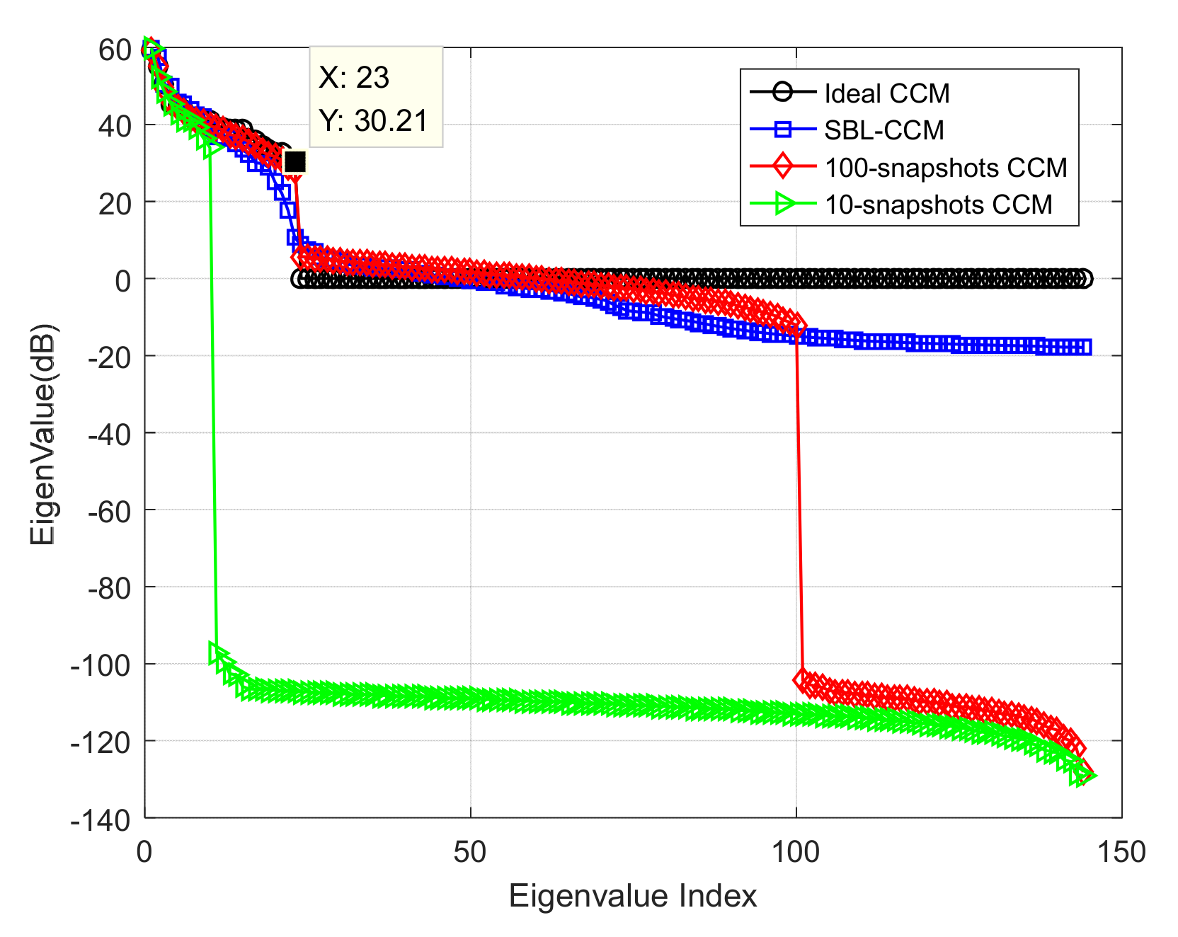
It is well known that the space scanned by the eigenvectors corresponding to large eigenvalues is the clutter subspace [12,22], so the number of large eigenvalues can reflect the accuracy of CNCM estimation. According to Brennan’s criterion [1], the number of large eigenvalues in this paper should be 23. Figure 6 clearly shows that the accuracy of estimating CNCM using 100 samples is much higher than using 10 samples, and the accuracy of estimating CNCM using the SBL algorithm in the single-sample case is somewhere in between.

Figure 6. Comparison of eigenspectra of ideal and estimated CNCM.

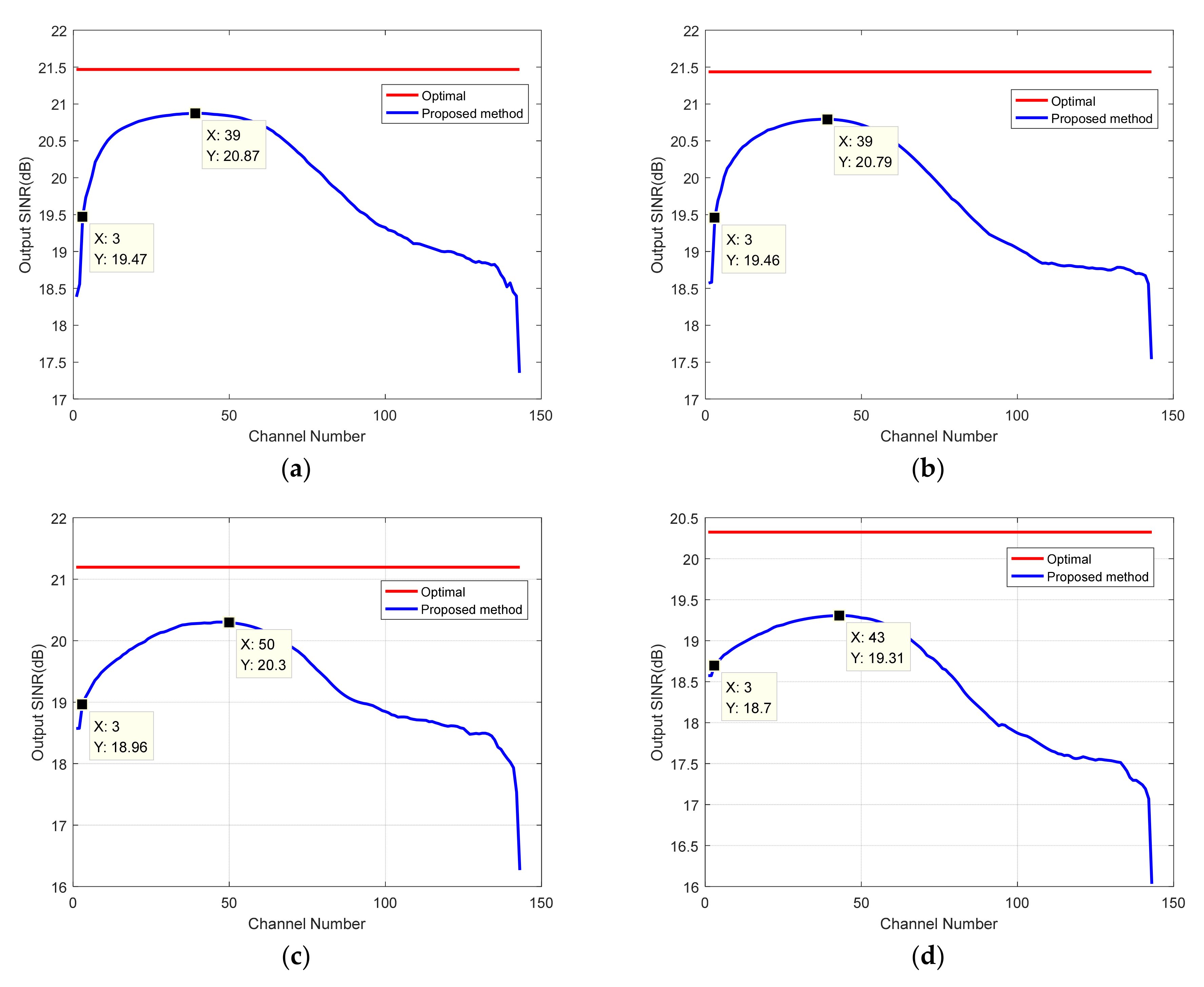
In addition, the performance of the proposed algorithm varies with the number of selected auxiliary channels under different target normalized Doppler frequencies, which are presented in Figure 7a–f. From Figure 7, We can clearly see that only 3–5 auxiliary channels are needed to achieve suboptimal clutter suppression performance, and using more channels not only takes a huge computational burden but also gains little performance improvement. It can also be found that the clutter suppression performance is rather degraded when too many auxiliary channels are used, which is due to the inaccurate CNCM estimation. Therefore, from the point of view of balancing algorithmic performance and computational complexity, it is wise to choose 3–7 auxiliary channels.

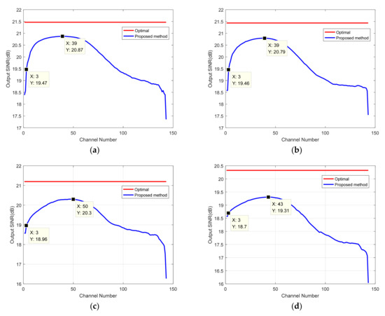
Figure 7. The SINR of the proposed algorithm varies with the number of auxiliary channels used. (a) $f_d=-0.5$; (b) $f_d=-0.3333$; (c) $f_d=-0.1667$; (d) $f_d=0.0833$; (e) $f_d=0.25$; (f) $f_d=0.4167$.

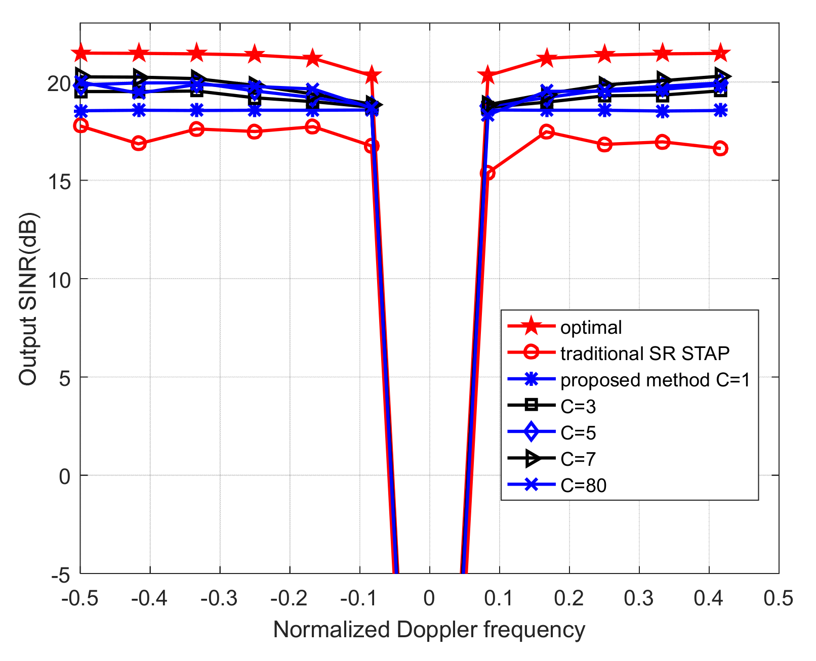
It should be noted that there is a total of $\left(MN-1\right)$ auxiliary channels to choose from. When all candidate channels are selected, the proposed algorithm degenerates into the traditional STAP algorithm based on sparse recovery (SR STAP), and naturally, there is no dimensionality reduction. The SINR of the proposed algorithm with different numbers of auxiliary channels is shown in Figure 8, where C represents the number of auxiliary channels selected. C = 1 indicates that the proposed algorithm selects only one auxiliary channel. From Figure 8, we can observe that the output SINR of the proposed algorithm is better than that of traditional SR STAP when only one auxiliary channel is used. Furthermore, we can observe that the SINR of the proposed algorithm with 80 auxiliary channels is approximately the same as that with 5 auxiliary channels but slightly lower than that with 7 auxiliary channels, which is consistent with the simulation results in Figure 7.

Figure 8. SINR comparison of the proposed method with C = 1,3,5,7,80 and the traditional SR STAP.

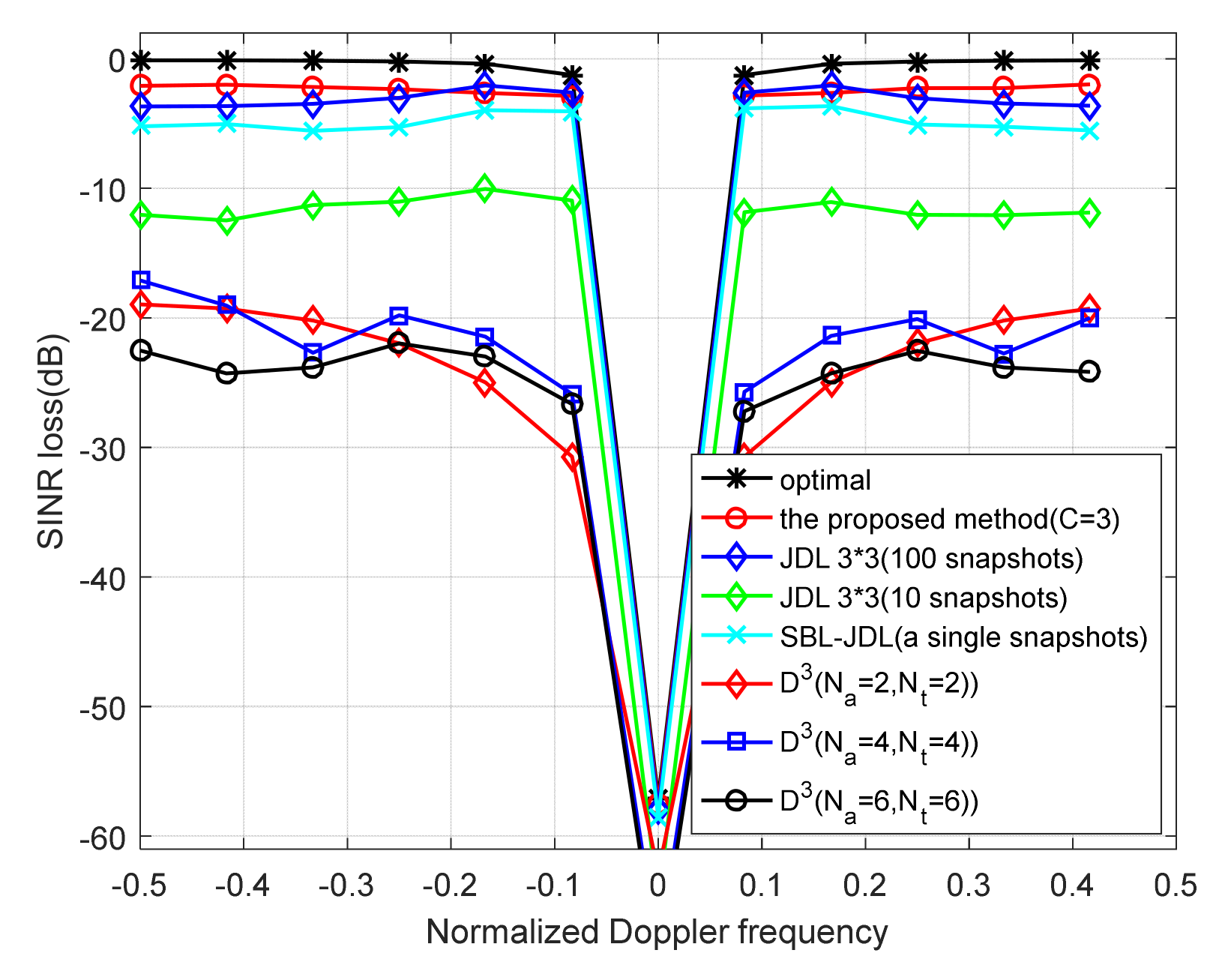
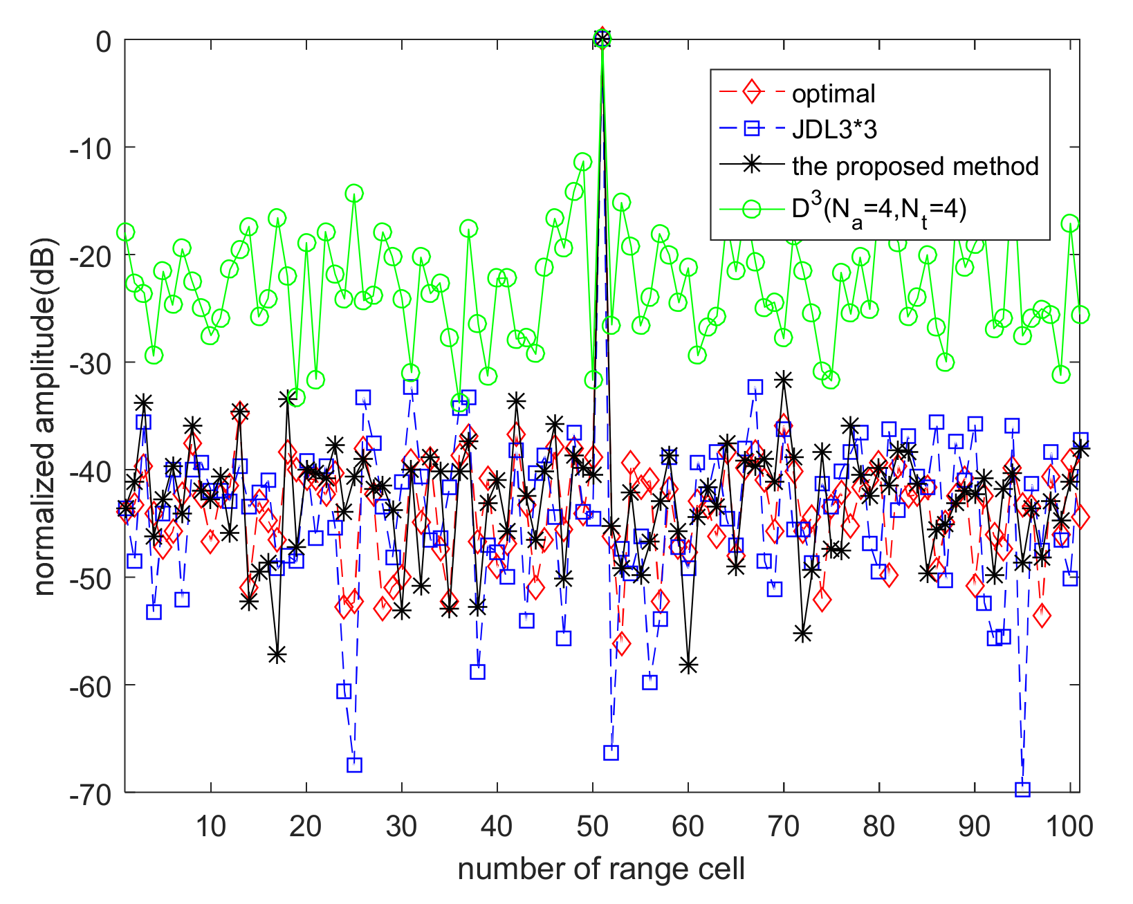
The comparison of the output SINR loss of the proposed algorithm with the best STAP [1], JDL [5] algorithm, and direct data domain (D3) algorithm [23] is shown in Figure 9. In the simulation of Figure 9, the number of auxiliary channels used by the proposed algorithm is 3, and the number of auxiliary channels used by the JDL algorithm is 8. Three scenarios for estimating the CNCM are considered: 100 samples, 10 samples, and the SBL algorithm, which uses only one sample to estimate the CNCM. In the simulation of the direct data domain algorithm, the lengths of the spatial and temporal sliding windows are 2, 4, and 6, respectively. The simulation results are shown in Figure 9, where it can be clearly seen that the JDL algorithm still has a larger output SINR loss than the proposed algorithm when using 100 samples. Moreover, the output SINR loss of the proposed algorithm is nearly 20 dB smaller than that of the direct data domain algorithm, which indicates that the proposed algorithm has better clutter suppression performance than the direct data domain algorithm.

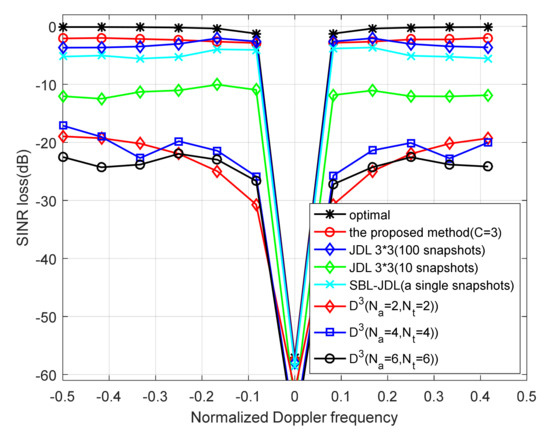
Figure 9. Clutter suppression performance comparison of several typical algorithms.

To illustrate the superiority of the proposed channel selection algorithm, we compare the output SINR loss of the SBL-JDL algorithm with that of the proposed algorithm. The SBL-JDL algorithm is a single-sample algorithm that obtains the CNCM by the SBL algorithm and then selects 8 auxiliary channels according to the JDL algorithm. The only difference between the SBL-JDL algorithm and the proposed algorithm is the method of selecting auxiliary channels. As can be seen in Figure 9, although the number of auxiliary channels used is less than that of the SBL-JDL algorithm, the proposed algorithm still has a better SINR loss than the SBL-JDL algorithm.

We also simulated the target detection performance of the optimum STAP, JDL algorithm (100 samples), direct data domain algorithm, and the proposed algorithm. The target is added to the $51\text{-}th$ range bin. The simulation results are shown in Figure 10. We can see that the proposed algorithm performs close to the optimal STAP and the JDL algorithm using 100 samples when the constant false alarm detector is used.

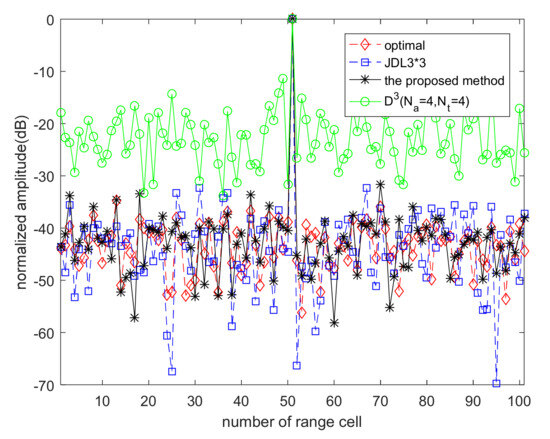
Figure 10. Comparison of adaptive beamforming output of several typical algorithms.

So far, we have been considering an ideal error-free clutter environment. In order to verify the robustness, we introduce the gain-phase (GP) error in the simulation experiments in Figure 11. According to [16,24], the clutter model with GP errors can be expressed as

$$x_{GP}=EDw+x_n$$

(49)

The GP error matrix $E$ can be expressed as

$$E=I_M\otimes diag\left({\left[e_1\exp \left(j{\phi }_1\right),e_2\exp \left(j{\phi }_2\right),\cdots ,e_N\exp \left(j{\phi }_N\right)\right]}^T\right)$$

(50)

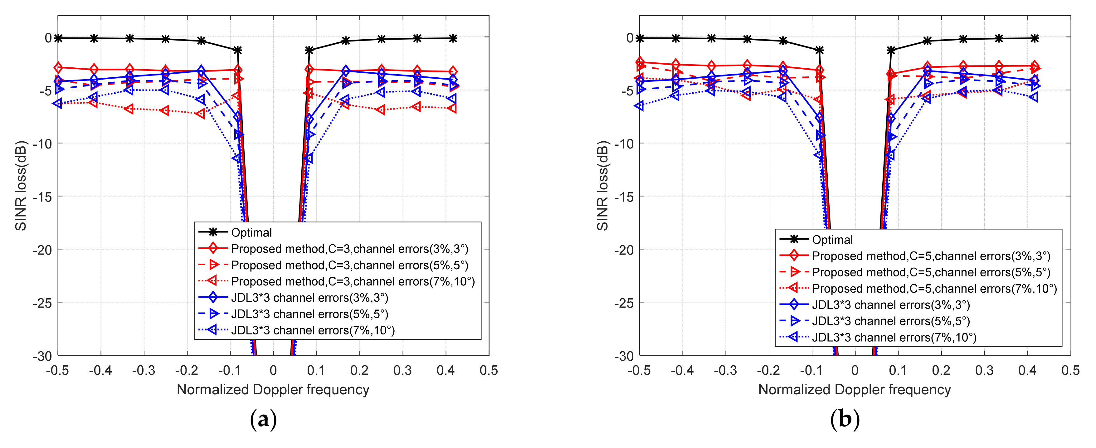
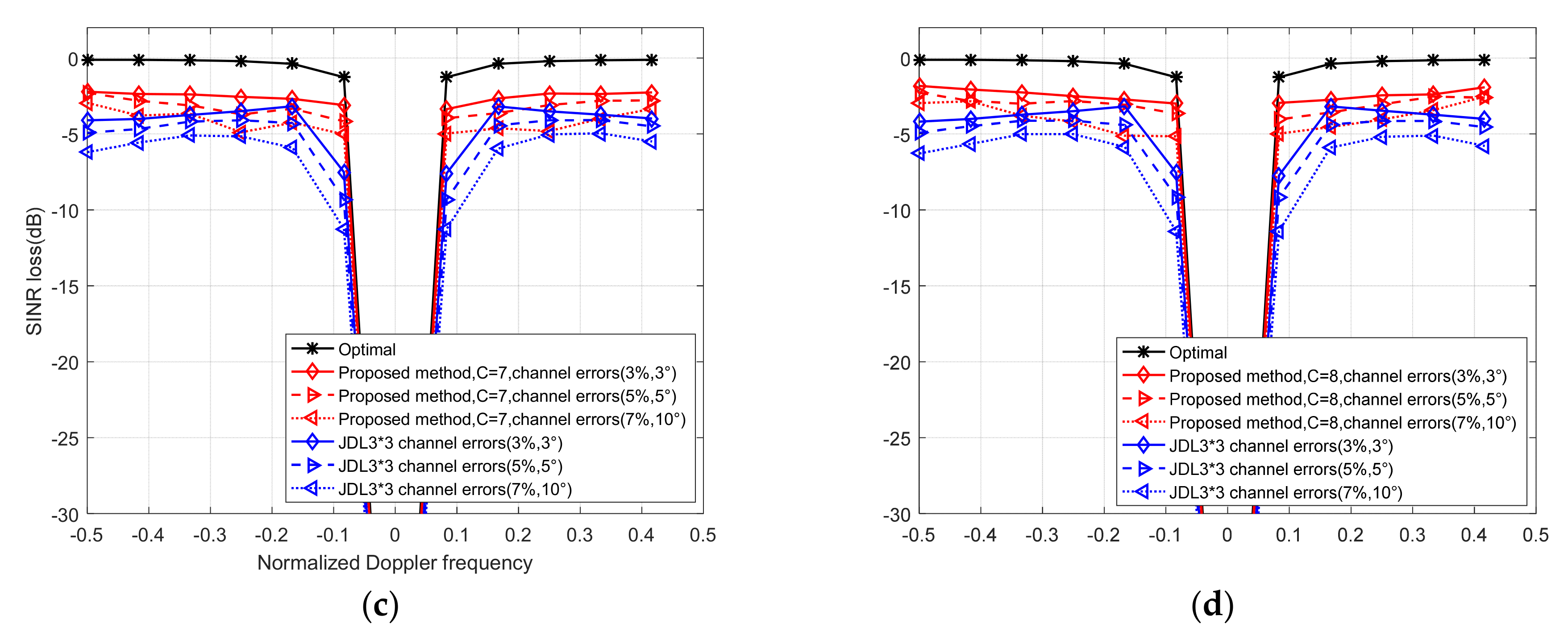
where $e_j$ and ${\phi }_j$ denote the amplitude error and phase error added to the $j\text{-}th$ array element, respectively. In Figure 11, the average fluctuation of the added amplitude error is 3%, 5%, and 7% of the amplitude without error, respectively. The average fluctuations of the added phase error are 3°, 5°, and 10°, respectively. The number of auxiliary channels used by the proposed algorithm is 3, 5, 7, and 8, while the number of auxiliary channels used by the JDL algorithm is always 8. In addition to this, the proposed algorithm uses only one sample, and the JDL algorithm uses 100 samples.

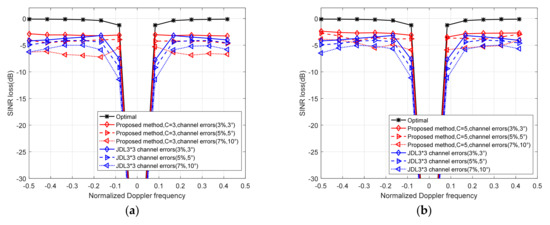
Figure 11. SINR loss of the proposed algorithm and JDL algorithm in the presence of GP error. (a) Proposed algorithm, C = 3; JDL, C = 8; (b) proposed algorithm, C = 5; JDL, C = 8; (c) proposed algorithm, C = 7; JDL, C = 8; (d) proposed algorithm, C = 8; JDL, C = 8.

The simulation results in Figure 11 show that the introduction of GP error degrades the performance of the proposed algorithm and the JDL algorithm, and the larger the GP error, the more the performance degrades. In addition, the output SINR loss of the proposed algorithm decreases as the number of auxiliary channels used increases. The proposed algorithm has no significant advantage over the JDL algorithm when only three auxiliary channels are used in the presence of GP errors, as can be seen in Figure 11a. From Figure 11b–d, gradually increasing the number of auxiliary channels used, the performance of the proposed algorithm gradually improves and outperforms the JDL algorithm. The proposed algorithm performs significantly better than the JDL algorithm when 7 or 8 auxiliary channels are used.

4.2. Performance Analysis Based on Measured Data

To further analyze the performance of the proposed algorithm, the proposed algorithm is applied to the Mountain-top data (t38pre01v1_cpi_6) in this subsection. The data were collected by the Lincoln Laboratory at the Massachusetts Institute of Technology [25]. The specific parameters of the Mountain-top dataset are shown in Table 3.

Table 3. The main parameter of Mountain-top dataset.

Parameters	Value
Array number	14
Pulses number	16
PRF	625 Hz
Bandwidth	500 kHz
Range cell number	403
Range cell of target	147
Azimuth angle of target	275°
Normalized Doppler frequency of target	0.25

This dataset contains a total of 403 range cells, and the target is located at the 147th range cell. Using the clutter data of all 403 range cells, the clutter covariance matrix is estimated as [2]

$$R_m=\frac{1}{403}{\displaystyle \sum _{i=1}^{403}{x}_i{x}_i^H}$$

(51)

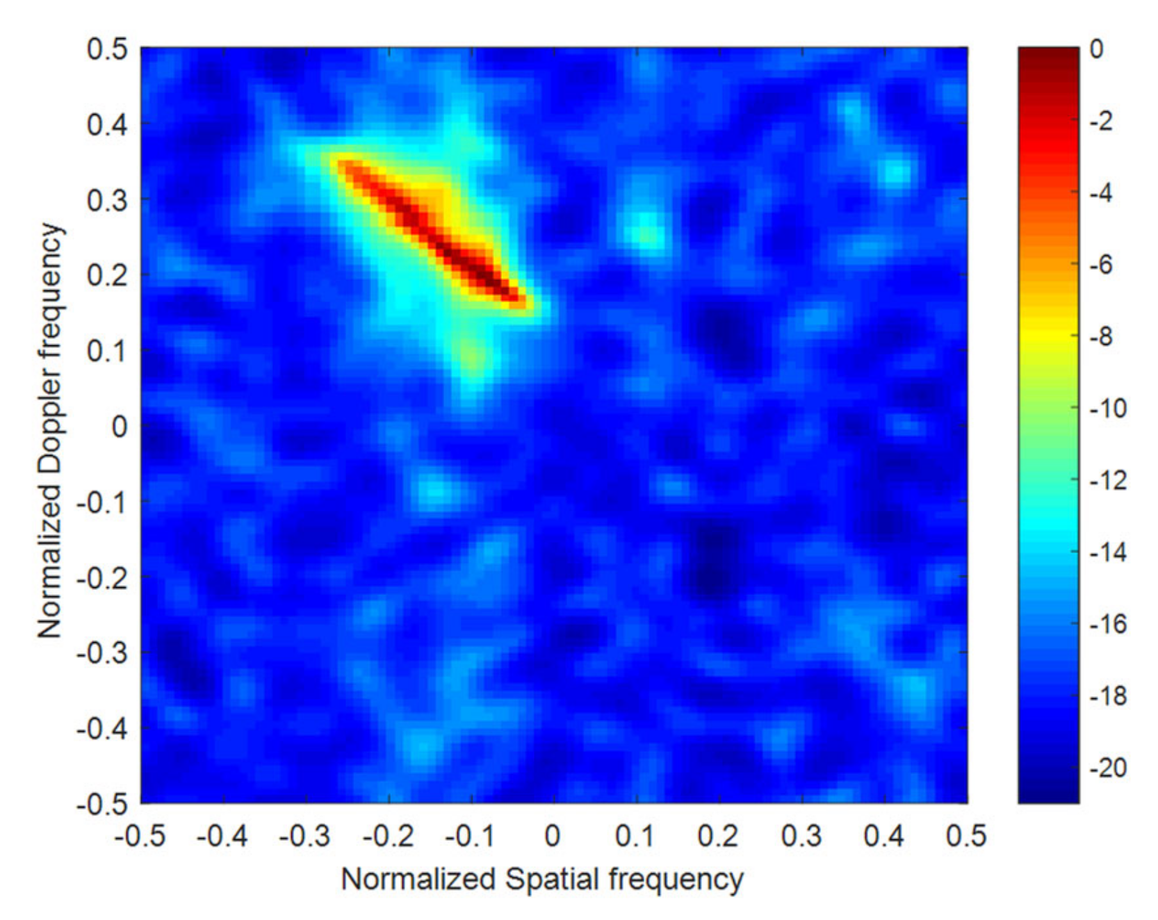
In Formula (51), $x_i$ represents the clutter data of the $i\text{-}th$ range cell. Using $R_m$ to calculate clutter Capon spectrum is shown in Figure 12.

Figure 12. Estimated clutter spectrum using all 403 range cells.

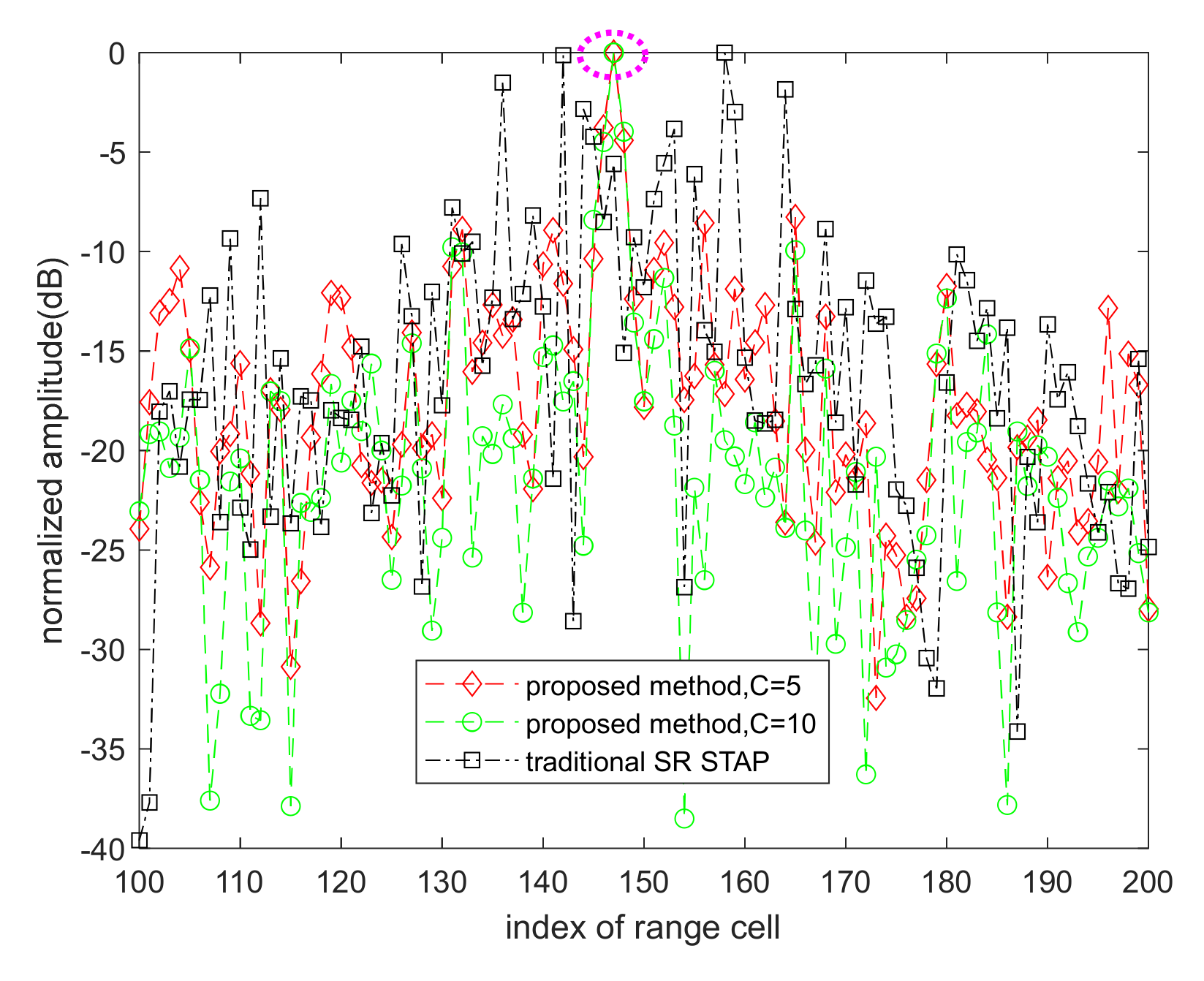
When the performance of the proposed algorithm is verified using the measured dataset, the sliding window method is used to detect the presence of the target along the range cell. In order to prevent the target energy leakage caused by the movement of the target from affecting the detection performance, four range cells on the left and right sides of the range cell under test are specified as protection cells. The clutter data of the fifth range cell on the left or right adjacent to the range cell under test are used as training samples for target detection according to the proposed algorithm. The detection results along the range cell are shown in Figure 13. In Figure 13, circled by a purple dashed ellipse, is the output energy of the range cell where the target is located. It can be seen from Figure 13 that the proposed algorithm can detect targets both when 5 channels and 10 channels are used. The difference between the two cases is that when 10 channels are used, the range cell without a target has less clutter remaining. Comparing the proposed algorithm with the traditional SR STAP algorithm, it can be seen that when only one training sample is used, the traditional SR STAP not only fails to detect the target but also generates a false alarm in the range cell without a target. It is obvious that the performance of traditional SR STAP will decrease significantly when the CCM estimation is not accurate, but the proposed algorithm can still maintain acceptable target detection performance.

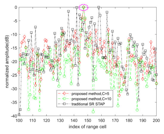
Figure 13. Output power against the range cell.

5. Conclusions

In this work, an angular Doppler domain reduced-dimension STAP algorithm based on SBL was proposed. First, the CNCM is estimated by the SBL algorithm using only one sample. Second, the RD matrix is designed using the estimated CNCM and the proposed angular Doppler channel selection algorithm. Finally, the estimated CNCM and the designed RD matrix are used to design an RD filter to process the data of the CUT and detect the target. The experimental results demonstrate that the proposed algorithm maintains suboptimal performance in extremely heterogeneous clutter environments where only one sample is available. Due to the high computational complexity of the currently popular efficient sparse recovery algorithms, in order to improve the real-time performance of the proposed algorithms, the future research direction is mainly focused on the fast and accurate sparse recovery algorithms suitable for airborne radar.

References

- Ward, J. Space-Time Adaptive Processing for Airborne Radar; Technical Report, 1015; MIT Lincoln Laboratory: Lexington, MA, USA, 1994. [Google Scholar]
- Reed, I.S.; Mallett, J.D.; Brennan, L.E. Rapid Convergence Rate in Adaptive Arrays. IEEE Trans. Aerosp. Electron. Syst. 1974, 10, 853–863. [Google Scholar] [CrossRef]
- Klemm, R. Adaptive airborne MTI: An auxiliary channel approach. In IEE Proceedings F (Communications, Radar and Signal Processing); IET Digital Library: London, UK, 1987; Volume 134, pp. 269–276. [Google Scholar]
- Dipietro, R.C. Extended factored space-time processing for airborne radar systems. In Proceedings of the Conference Record of the Twenty-Sixth Asilomar Conference on Signals, Systems & Computers, Pacific Grove, CA, USA, 26–28 October 1992; IEEE Computer Society: Pacific Grove, CA, USA, 1992; pp. 425–430. [Google Scholar]
- Wang, H.; Cai, L. On Adaptive Spatial-Temporal Processing for Airborne Surveillance Radar Systems. IEEE Trans. Aerosp. Electron. Syst. 1994, 7, 660–670. [Google Scholar] [CrossRef]
- Sun, K.; Zhang, H.; Li, G.; Meng, H.; Wang, X. A novel STAP algorithm using sparse recovery technique. In Proceedings of the 2009 IEEE International Geoscience and Remote Sensing Symposium, Cape Town, South Africa, 12–17 July 2009. [Google Scholar]
- Yang, Z.; Li, X.; Wang, H.; Nie, L. Sparsity-Based Space-Time Adaptive Processing Using Complex-Valued Homotopy Technique. In Proceedings of the 2013 IEEE Radar Conference, Ottawa, ON, Canada, 29 April–3 May 2013. [Google Scholar]
- Sen, S. Low-Rank Matrix Decomposition and Spatial-Temporal Sparse Recovery for STAP Radar. IEEE J. Sel. Top. Signal Process. 2015, 12, 1510–1523. [Google Scholar] [CrossRef]
- Duan, K.; Wang, Z.; Xie, W. Sparsity-based STAP algorithm with multiple measurement vectors via sparse Bayesian learning strategy for airborne radar. IET Signal Process. 2016, 9, 544–553. [Google Scholar] [CrossRef]
- Wang, Z.; Wang, Y.; Gao, F. Clutter nulling space-time adaptive processing algorithm based on sparse representation for airborne radar. IET Radar Sonar Navig. 2017, 11, 177–184. [Google Scholar]
- Feng, W.; Guo, Y.; He, X. Jointly Iterative Adaptive Approach Based Space Time Adaptive Processing Using MIMO Radar. IEEE Access. 2018, 6, 26605–26616. [Google Scholar] [CrossRef]
- Wang, D.; Wang, T.; Cui, W.; Zhang, X. A Clutter Suppression Algorithm via Enhanced Sparse Bayesian Learning for Airborne Radar. IEEE Sens. J. 2023, 5, 10900–10911. [Google Scholar] [CrossRef]
- Fa, R.; De Lamare, R.C. Reduced-Rank STAP Algorithms using Joint Iterative Optimization of Filters. IEEE Trans. Aerosp. Electron. Syst. 2011, 7, 1668–1684. [Google Scholar] [CrossRef]
- Sun, K.; Meng, H.; Wang, Y. Direct Data Domain STAP using Sparse Representation of Clutter Spectrum. Signal Process. 2011, 4, 2222–2236. [Google Scholar] [CrossRef]
- Guo, Y.; Liao, G.; Feng, W. Sparse Representation Based Algorithm for Airborne Radar in Beam-Space Pose-Doppler Reduced-Dimension Space-Time Adaptive Processing. IEEE Access 2017, 4, 5896–5903. [Google Scholar] [CrossRef]
- Yang, Z.; de Lamare, R.C.; Li, X. L1-Regularized STAP Algorithms with a Generalized Sidelobe Canceler Architecture for Airborne Radar. IEEE Trans. Signal Process. 2012, 2, 674–686. [Google Scholar] [CrossRef]
- Zhang, W.; He, Z.; Li, J. A Method for Finding Best Channels in Beam-Space Post-Doppler Reduced-Dimension STAP. IEEE Trans. Aerosp. Electron. Syst. 2014, 1, 254–264. [Google Scholar] [CrossRef]
- Tipping, M.E. Sparse Bayesian Learning and the Relevance Vector Machine. J. Mach. Learn. 2001, 1, 211–244. [Google Scholar]
- Shutin, D.; Buchgraber, T.; Kulkarni, S.R. Fast Variational Sparse Bayesian Learning with Automatic Relevance Determination for Superimposed Signals. IEEE Trans. Signal Process. 2011, 12, 6257–6261. [Google Scholar] [CrossRef]
- Zhou, W.; Zhang, H.-T.; Wang, J. An efficient Sparse Bayesian Learning Algorithm Based on Gaussian-Scale Mixtures. IEEE Trans. Neural Netw. Learn. Syst. 2021, 1, 3065–3078. [Google Scholar] [CrossRef] [PubMed]
- Zhang, W.; An, R.; He, N. Reduced Dimension STAP Based on Sparse Recovery in Heterogenous Clutter Environments. IEEE Trans. Aerosp. Electron. Syst. 2020, 2, 785–795. [Google Scholar] [CrossRef]
- Haimovich, A.M.; Berin, M. Eigenanalysis-based space-time adaptive radar: Performance analysis. IEEE Trans. Aerosp. Electron. Syst. 1997, 10, 1170–1179. [Google Scholar] [CrossRef]
- Sarkar, T.K.; Wang, H.; Park, S. A deterministic least-squares approach to space-time adaptive processing (STAP). IEEE Trans. Antennas Propag. 2001, 2, 91–103. [Google Scholar] [CrossRef]
- Wang, D.; Wang, T.; Cui, W. Adaptive Support-Driven Sparse Recovery STAP Method with Subspace Penalty. Remote Sens. 2022, 14, 4463. [Google Scholar] [CrossRef]
- Titi, G.W.; Marshall, D.F. The ARPA/NAVY mountaintop program: Adaptive signal processing for airborne early warning radar. In Proceedings of the 1996 IEEE International Conference on Acoustics, Speech, and Signal Processing Conference, Atlanta, GA, USA, 9 May 1996; IEEE: Piscataway, NJ, USA, 1996; Volume 5, pp. 1165–1168. [Google Scholar]
Disclaimer/Publisher’s Note: The statements, opinions and data contained in all publications are solely those of the individual author(s) and contributor(s) and not of MDPI and/or the editor(s). MDPI and/or the editor(s) disclaim responsibility for any injury to people or property resulting from any ideas, methods, instructions or products referred to in the content. |
© 2024 by the authors. Licensee MDPI, Basel, Switzerland. This article is an open access article distributed under the terms and conditions of the Creative Commons Attribution (CC BY) license (https://creativecommons.org/licenses/by/4.0/).