Article

Comprehensive Ecological Risk Changes and Their Relationship with Ecosystem Services of Alpine Grassland in Gannan Prefecture from 2000–2020

1
State Key Laboratory of Herbage Improvement and Grassland Agro-Ecosystems, Key Laboratory of Grassland Livestock Industry Innovation, Ministry of Agriculture, College of Pastoral Agriculture Science and Technology, Lanzhou University, Lanzhou 730000, China
2
Linze Inland River Basin Research Station, Chinese Ecosystem Network Research, Key Laboratory of Ecohydrology of Inland River Basin, State Key Laboratory of Cryospheric Science, Northwest Institute of Eco-Environment and Resources, Chinese Academy of Sciences, Lanzhou 730000, China
3
Institute of Environment and Ecology, Tsinghua Shenzhen International Graduate School, Tsinghua University, Shenzhen 518055, China
*
Author to whom correspondence should be addressed.
Remote Sens. 2024, 16(12), 2242; https://doi.org/10.3390/rs16122242
Submission received: 16 April 2024 / Revised: 2 June 2024 / Accepted: 11 June 2024 / Published: 20 June 2024

Abstract

:
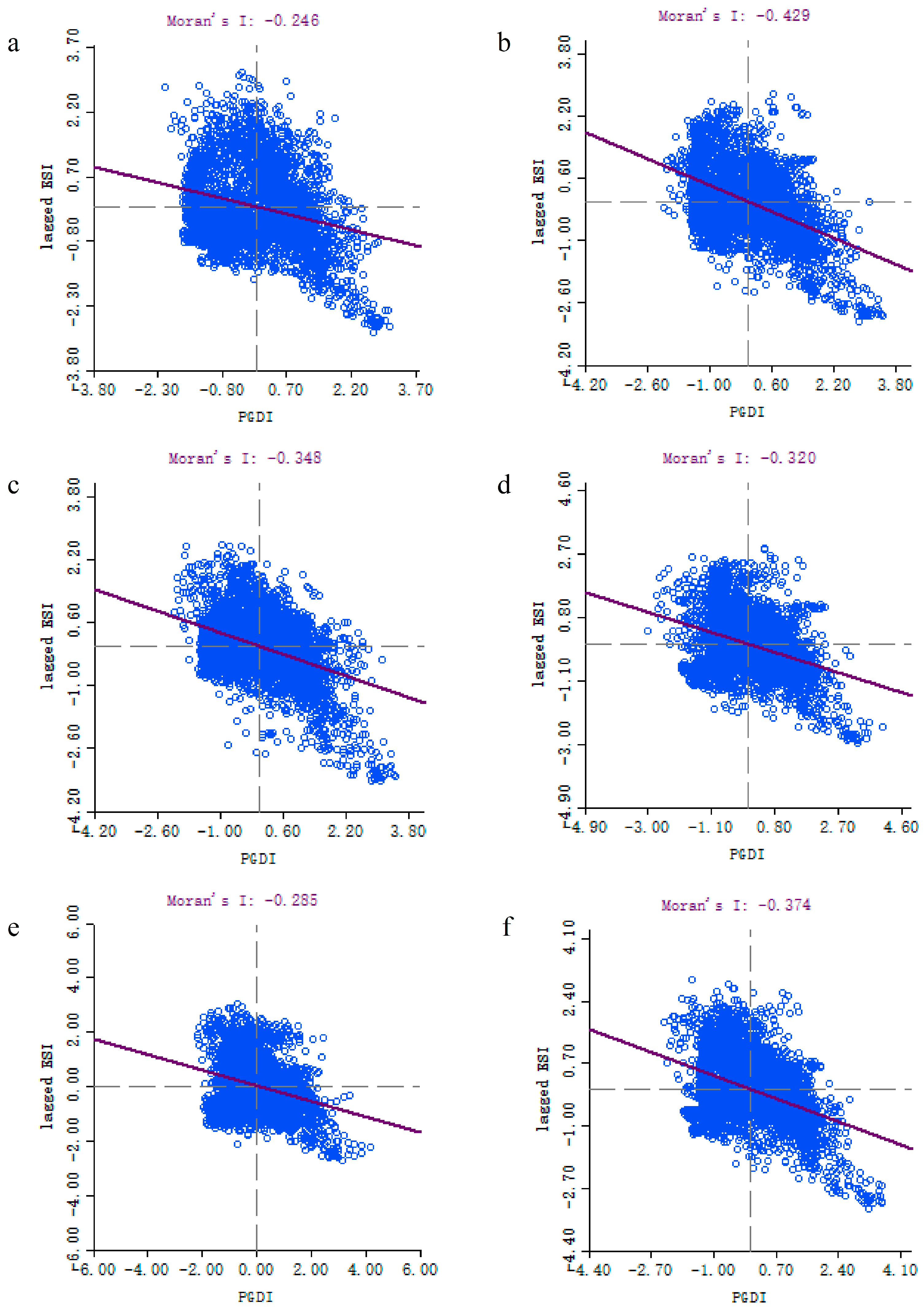
Alpine grassland is one of the most fragile and sensitive ecosystems, and it serves as a crucial ecological security barrier on the Tibetan Plateau. Due to the combined influence of climate change and human activities, the degradation of the alpine grassland in Gannan Prefecture has been increasing recent years, causing increases in ecological risk (ER) and leading to the grassland ecosystem facing unprecedented challenges. In this context, it is particularly crucial to construct a potential grassland damage index (PGDI) and assessment framework that can be used to effectively characterize the damage and risk to the alpine grassland ecosystem. This study comprehensively uses multi-source data to construct a PGDI based on the grassland resilience index, landscape ER index, and grass–livestock balance index. Thereafter, we proposed a feasible framework for assessing the comprehensive ER of alpine grassland and analyzed the responsive relationship between the comprehensive ER and comprehensive ecosystem services (ESs) of the grassland. There are four findings. The first is that the comprehensive ER of the alpine grassland in Gannan Prefecture from 2000–2020 had a low distribution in the southeast and a high distribution trend in the northwest, with medium risk (29.27%) and lower risk (27.62%) dominating. The high-risk area accounted for 4.58% and was mainly in Lintan County, the border between Diebu and Zhuoni Counties, the eastern part of Xiahe County, and the southwest part of Hezuo. Second, the comprehensive ESs showed a pattern of low distribution in the northwest and high distribution in the southeast. The low and lower services accounted for only 9.30% of the studied area and were mainly distributed in the west of Maqu County and central Lintan County. Third, the Moran’s index values for comprehensive ESs and ER for 2000, 2005, 2010, 2015, and 2020 were −0.246, −0.429, −0.348, −0.320, and −0.285, respectively, thereby indicating significant negative spatial autocorrelation for all aspects. Fourth, ER was caused by the combined action of multiple factors. There are significant differences in the driving factors that affect ER. Landscape index is the first dominant factor affecting ER, with q values greater than 0.25, followed by DEM and NDVI. In addition, the interaction between diversity index and NDVI had the greatest impact on ER. Overall, this study offers a new methodological framework for the quantification of comprehensive ER in alpine grasslands.

Graphical Abstract

1. Introduction

Grasslands are among the most extensively distributed vegetation types globally, and they are an important component of terrestrial ecosystems that have significant ecological, economic, and social value. They are also essential for conserving biodiversity and maintaining balance in ecosystems [1,2,3]. Alpine grasslands are the dominant ecosystem on the Tibetan Plateau, covering more than 60% of the entire area [4]. In recent years, however, these grasslands have experienced significant extreme climate events, warming, and drought that have altered their phenology [5] and reduced their livestock-carrying capacity and primary productivity [6,7,8]. The grassland ecosystem in Gannan Tibetan Autonomous Prefecture (Gannan Prefecture) is an important component of the Tibetan Plateau’s grassland ecosystems and a crucial ecological security barrier in Northwestern China. Recently, intensified human activities and global climate change have led to the grassland ecosystem in Gannan Prefecture facing unprecedented threats. Meanwhile, many negative phenomena, such as grassland degradation, soil erosion, and biodiversity reduction, are frequently seen [9,10], causing great difficulties for the local natural environment and socioeconomic development. Therefore, there is an urgent requirement to accurately assess the ecological risk (ER) of alpine grassland in Gannan Prefecture and to understand the changes in ecosystem services (ESs).
ER typically refers to the pressure exerted by external factors on the function and structure of ecosystems, and it describes the potential adverse influences of both natural disasters and human activities on ecosystems [11,12]. ER assessment (ERA) is a tool that effectively measures and evaluates the negative consequences and influences of natural disasters, anthropogenic coercion, and environmental pollution on local ecosystems. ERA is currently an important basis for resource management, environmental restoration, and decision-making about ecological construction in China [13,14,15]. It is an effective measure for identifying and mitigating ecosystem degradation [11,16]. Most studies on ERA have focused on single-indicator risk sources (i.e., rodent infestation, vegetation cover, soil erosion, and landscape ecological risk). For instance, pollution risk factors for wetland ecosystems were used to develop an ERA approach for freshwater wetlands [17], and land use change in the Zoige Plateau was used to analyze the landscape ecological risk of alpine wetland ecosystems [18].
However, the factors that affect grassland ecosystems are diverse and complex, and evaluating the ER of grasslands based on a single risk source often has certain limitations. For this reason, some studies have proposed multi-indicator comprehensive evaluation methods for assessing ER. The ERA of the Luanhe River Basin comprehensively considered chemical and biological indicators to construct the ER index [19], and in the study of wetland ER, multiple indicators such as precipitation, temperature, and wetland area were used to evaluate the wetland ER in the Beijing–Tianjin–Hebei region for six periods from 1990 to 2015 to establish a reasonable and scientific wetland ER evaluation system [20].
As the environmental and ecological problems of the alpine grassland in Gannan Prefecture have received increasing attention, scholars have accessed the ER from different aspects in recent years. For instance, in the study of the ecological environment of the Gannan Plateau, 30 indicators such as hydro-meteorology, ecological environment, and surface disturbance were used for the ERA of the Gannan Plateau [21], and in the ERA of Gannan, multiple indicators of natural and human factors were used to analyze the risks of alpine grassland ecosystems [22], both of which provided important information for the ecological environment research on the Gannan alpine grassland. Nevertheless, there is a relative lack of research into ERA methods, especially in terms of alpine grassland ecosystems. In addition, Chen et al. proposed a holistic view of risk management and assessment, arguing that ERA should consider social systems, ecosystems, and their interactions [23]. Currently, ESs have been integrated into the ERA framework by many researchers to compensate for the shortcomings of ESs’ risk losses.
People directly or indirectly derive benefits from ESs, which emphasize the significance of the natural environment for human societies. An ESs assessment describes ecosystems’ service capacity to human society, with the general evaluation indicators being soil conservation (SC), water yield (WY), and habitat quality (HQ), amongst others [24,25]. As remote sensing, geographic information systems (GIS), and other technologies have continued to mature, research on ESs has entered a new stage. Modeling methods (i.e., InVEST, SoLVES, and ARIE) are currently among those widely used to assess ESs because of their advantages, including low costs and high accuracies [26]. In particular, the InVEST model is favored by many scholars. For example, in the exploration of spatial heterogeneity, trade-offs, synergy, and driving factors in the Loess Plateau, CASA, InVEST, and RUSLE models were used to assess the ESs of the WY, SC, and carbon storage in the Loess Plateau from 2000 to 2018 [27], and in the study of water-related services in the Tungabhadra, the author used the InVEST water quantity model to analyze the impacts of climate change on water-related services (e.g., hydropower and water quantity) [28]. In fact, in recent years, there has been a rising trend of studies on ESs and ER, as it is crucial to reduce ER and improve ESs to protect grassland ecological environments [29]. At present, most ESs assessment studies on the alpine grassland in Gannan focus on the inherent value of grassland ESs [30,31]. Moreover, the majority of the studies start from a single risk source, and relatively few have carried out comprehensive ERAs that consider the health status of the grassland, changes in landscape patterns, and human factors, as well as the spatial distribution of ESs and ER during the study period. Furthermore, as there is no strictly synergistic relationship between the spatial ranges and research scopes of ESs and ER, a systematic analysis of the relationship and responses between the two is still necessary [32].
The exploration of the driving factors of ER is also a current research hotspot. Understanding the driving factors of ER is the focus of current research, and it is very important for making reasonable regional assessments [33]. Geodetector is a statistical tool designed by Wang et al. [34] that can efficiently detect geographic spatial heterogeneity and explore its driving forces. In recent years, many researchers have used this technology to conduct extensive studies on natural and human factors and have gained a deeper understanding of the driving mechanisms of ER. The relationship between DEM, slope, precipitation, temperature, landscape pattern, population density, other factors, and ER has received extensive attention from scholars [35,36,37]. In addition, Geodetector can better detect influencing factors and explain their interactions [38].
In summary, there is a relative lack of research using ecosystems as carriers in ERA, especially on the fragile ecosystems of alpine grasslands. Moreover, there are relatively few studies that comprehensively consider grassland health, landscape patterns changes, human factors, and the spatial distribution of ESs and ER. Therefore, taking Gannan Prefecture as the study area, this paper proposes a comprehensive ERA framework that is based on the health status of the grassland as well as changes in landscape patterns and human factors to determine the relationship between ER and ESs in this area for 2000, 2005, 2010, 2015, and 2020, thereby providing insights into how Gannan’s grassland ecosystem can be managed. The specific objectives of this study are: (1) to build a potential grassland damage index (PGDI) based on grassland resilience, landscape ER, and a grass–livestock balance index while analyzing the spatiotemporal distribution characteristics of the comprehensive ER of grassland in Gannan Prefecture; (2) to construct an integrated ecosystem service index based on the three ESs of HQ, WY, and SC in addition to analyzing the spatiotemporal distribution characteristics of the alpine grassland ecosystem’s comprehensive ESs in Gannan Prefecture; (3) to determine the association between ER and ESs using Moran’s index, and (4) to analysis the driving factors of ER in Gannan Prefecture based on Geodetector.

2. Materials and Methods

2.1. Study Area

Gannan Prefecture is in the northeast of the Tibetan Plateau and is a significant water conservation region, covering a total area of 45,000 km2, with an average precipitation of 370~930 mm and an average annual temperature ranging from 0.6~2.3 °C (Figure 1). It has a vast grassland area, accounting for approximately 70.28% of the total area of the entire region, with the types mainly comprising alpine meadows and alpine shrub meadows [39]. Grasslands have a crucial function in livestock production, which is the main income of local herders. In recent years, the grassland ecosystem in Gannan Prefecture has been greatly damaged, and the ER has been increasing, seriously affecting local herders’ lives and economic situations [40].

2.2. Data Collection and Preprocessing Processes

The data employed in this study include remote sensing and basic geographic and statistical data. Table 1 lists the descriptions, sources, types, and formats of the data. The Landsat imagery was acquired from the Google Earth Engine (GEE) platform (with less than 60% cloud), and it was pre-processed through de-clouding, splicing, and masking. The meteorological data (temperature and precipitation data) come from the National Meteorological Information Center, including daily observation data from 10 meteorological stations in Gannan Prefecture and its surrounding areas. All the spatial data’s projections were set to WGS_1984_UTM_Zone_48_N, and all the data were resampled onto 30 m grid cells.

2.3. Methods

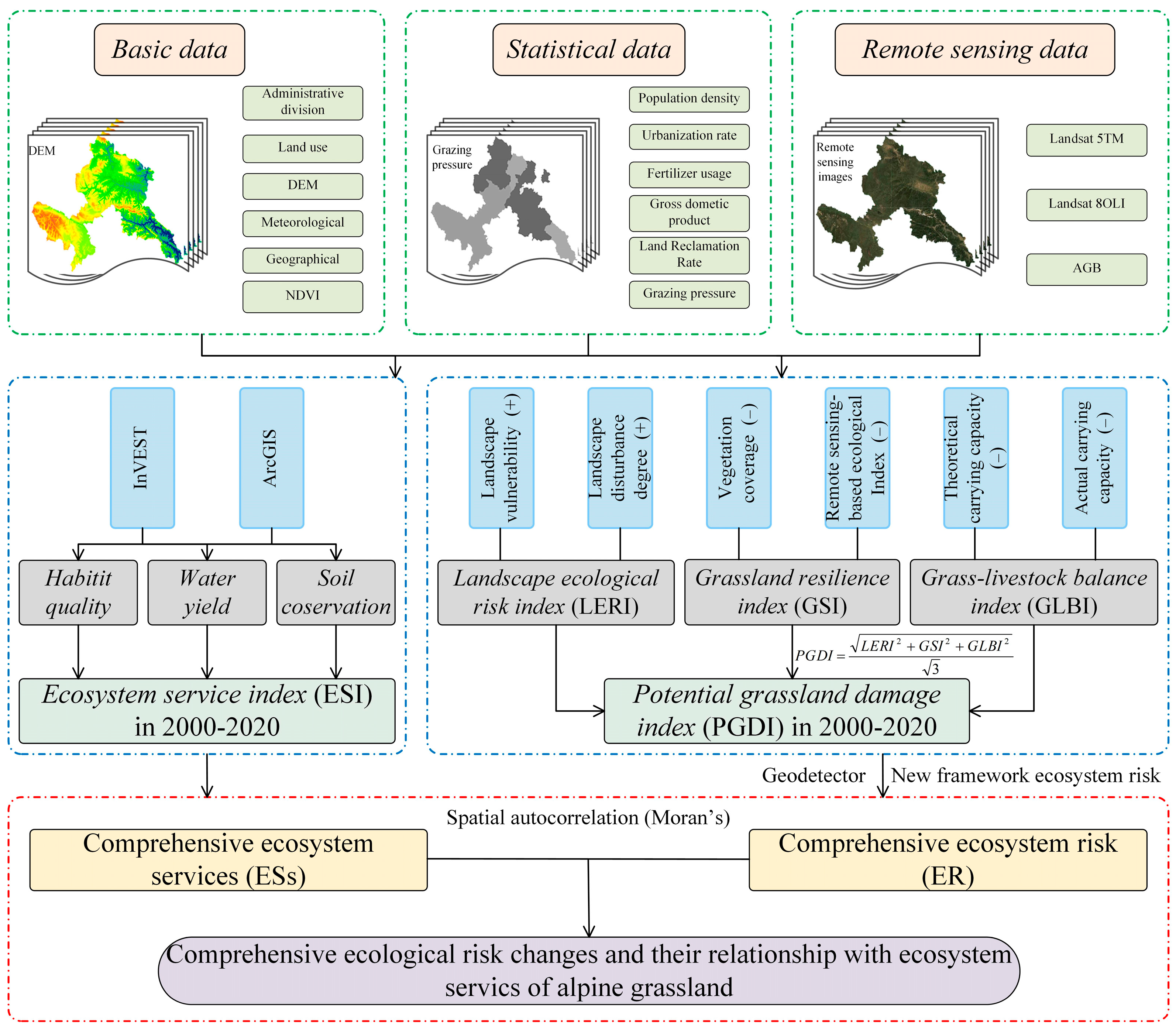
The research framework of this study is shown in Figure 2. First, we collected and preprocessed data from multiple sources (including basic data, statistical data, and satellite imagery data) necessary for the analysis using ArcGIS 10.6 and Google Earth Engine (GEE). Second, we constructed the potential grassland damage index (PGDI) that was established using the grassland resilience index (GRI), landscape ecological risk index (LERI), and grass–livestock balance index (GLBI). Then, we analyzed the spatiotemporal distribution characteristics of the ecosystem service index (ESI) and PGDI from 2000 to 2020. Finally, we explored the response relationship between ER and ESs based on a spatial autocorrelation analysis and analyzed the driving factors of ER using Geodetector.

2.3.1. Estimation of an Ecosystem Service Index

Considering the current situation of the grassland ecosystem in Gannan Prefecture, this study systematically evaluated the three services of HQ, WY, and SC based on land use as well as socio-economic and meteorological data, and we analyzed their spatiotemporal variations using ArcGIS 10.2 and the InVEST model. The calculation methods and data processing results of the three ESs are shown in Appendix A.
Moreover, this study constructed an ecological service index (ESI) to comprehensively measure the level of alpine grassland ESs in Gannan Prefecture. ESI should be calculated on the premise that the parameters are dimensionless to avoid the influence of dimensions [41]. Therefore, referring to relevant studies [42,43,44], various services were standardized using Formulas (2) and (3). The standardized ESI was then used to characterize the total amount of ESs herein, with the specific calculation formula being as follows:
E S I = i = 1 3 E S i
The positive effect indicators were standardized. The formula is as follows:
y i j = x i j x m i n x m a x x m i n
The negative effect indicators were standardized. The formula is as follows:
y i j = x m a x x i j x m a x x m i n
where ESI represents the Comprehensive Ecosystem Service Index, ES’i is the standardized value of the i-th ecosystem service, X m i n is the minimum value of a certain indicator, X i j represents the initial value of the j-th indicator for the i-th category, and X m a x is the maximum value of a certain indicator.
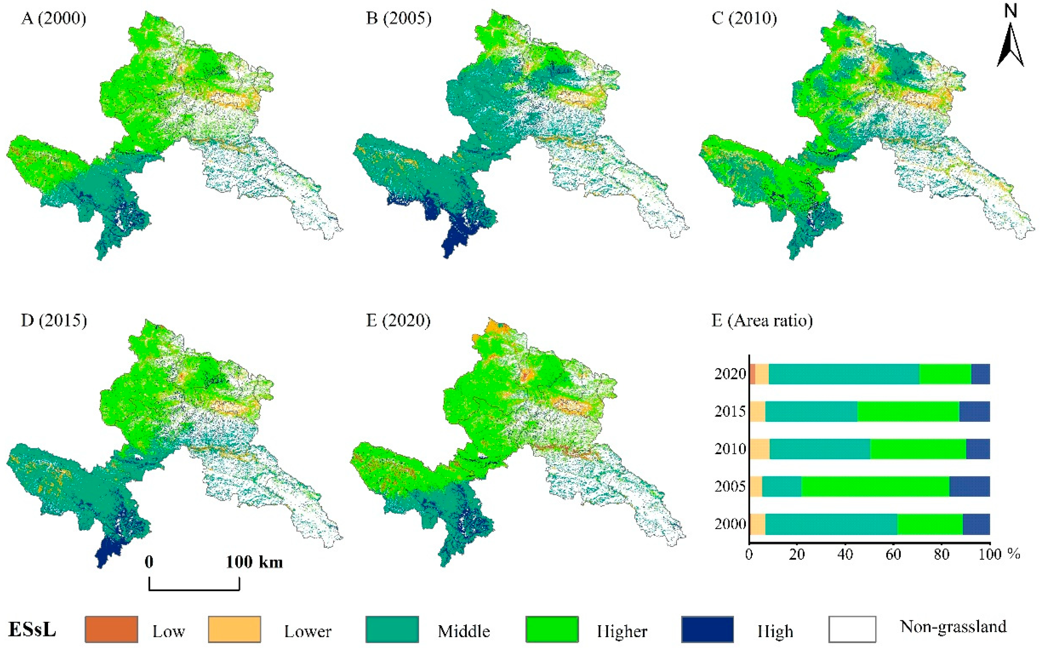
To analyze the spatiotemporal distribution differences of the ESs, considering the specific conditions in Gannan, this study used the Jenks natural breakpoint classification method [45] to divide the ESI into five levels; that is, low (ESI ≤ 0.20), lower (0.20 < ESI ≤ 0.30), middle (0.30 < ESI ≤ 0.40), higher (0.40 < ESI ≤ 0.50), high (ESI > 0.50).

2.3.2. The Calculation of the PGDI

(1)
GRI
Ecological resilience is an ecosystem’s ability to adapt and recover from risks, defined as the system’s ability to absorb or resist perturbations before reaching a transition threshold [46,47]. Generally, if the quality of grassland vegetation coverage is high, the grassland ecology and GRI will be of a higher quality. Therefore, a combination of remote sensing ecological index (RSEI) and fractional vegetation coverage (FVC) was used to calculate the GRI as follows:
G R I = W 1 · F V C + W 2 · R S E I
where W1 and W2 represent the weights of the FVC and RSEI, respectively. To maintain the neutrality of the results, the weights had an equal value of 0.5.
FVC is an important variable that describes vegetation quality and reflects changes in ecosystems. It directly reflects natural ecosystems’ environmental conditions and plays an important role in reducing ER [48,49]. FVC is defined as the ratio of the vertical projection of vegetation to the total statistical surface area, measured as a percentage [50,51]. This study combines the dimidiate pixel model to calculate FVC:
F V C = N D V I N D V I s o i l N D V I v e g N D V I s o i l
In the formula, FVC is the fractional vegetation coverage, and NDVIveg and NDVIsoil are the NDVI values of all vegetation-covered pixels and pure bare land pixels, respectively. In practical applications, NDVI histogram statistics are commonly used to obtain NDVIveg and NDVIsoil values with the given confidence intervals.
RSEI is an indicator that uses remote sensing data to objectively and quickly assess the regional ecological environment’s quality. Because of this, it is commonly used in ecological status evaluation [29,52]. This study references Xiong’s methods for calculating the RSEI [53]. The calculation is as follows:
R S E I = f G r e e n n e s s , H e a t , W e t n e s s , D r y n e s s
In the formula, Wetness, Greenness, Heat, and Dryness represent the humidity index, greenness index, heat index, and dryness index, respectively. These indicators were calculated according to [54].
(2)
The LERI
The LERI represents the degree in disturbance of different landscapes and is one of the most fundamental branches of ER [55]. It focuses on evaluating internal vulnerability and external disturbance [56]. This study combined the actual situation with relevant literature [57] and used the landscape vulnerability index and landscape interference index to calculate LERI [58]. The formula is as follows:
L E R I = i = 1 n A k i A k × R i
R i = E i · F i
E i = a C i + b C i + c D i
C i = n i A i
N i = A 2 A i × n i A
D i = Q i + M i 4 + L i 2
In this formula, Ri is the landscape loss index of the i-th landscape, Aki is the area of the i-th landscape in the k-th risk unit, Ei is the i-th land use type, Ci is the degree of landscape fragmentation, Fi is the landscape vulnerability index, A is the total area of the landscape, Ni is the degree of landscape separation, Ai is the total area of landscape type I, Di is the degree of landscape dominance, ni is the number of patches of landscape type I, Qi is the ratio of the number of units of type I land use type to the total number of units, and Li is the ratio of the i-th landscape patch area to the total patch area. the weight values of each landscape pattern index are represented by a, b, and c. According to previous research [59,60], the weights are allocated values of 0.5, 0.3, and 0.2, respectively.
(3)
The GLBI
The GLBI is an index that measures the dynamic equilibrium state of pasture and foraging livestock in a certain area and over a period of time [9,61]. It is calculated using the following formula:
G L B I = p c c S R P C C × 100
S R = N i · K i
P C C = i = 1 n A G B × A × H × U l u s × D
where GLBI is the grass–livestock balance index capacity, SR is the actual livestock-carrying capacity, Ni is the annual number of livestock (heads) of the i-th livestock, PCC is the theoretical livestock-carrying capacity, and Ki is the sheep unit conversion coefficient of the i-th livestock. AGB is the edible grass yield of the grassland, A represents the usable area coefficient of the grassland, H represents the edible grass conversion coefficient of the grassland, U represents the rational utilization coefficient of grazing grassland in the alpine grassland, lus represents the daily food intake of sheep per unit of sheep, calculated based on a daily consumption of 1.8 kg of hay by livestock, and D represents the time for grazing or raising on the grassland.
(4)
The PGDI
We hypothesize that if the health of the grassland in a grid significantly declines during a certain period, the risk of damage to the grassland in that grid will be the highest at the end of that period, when the extent of damage to the landscape pattern and human influence factors are greatest. Using inter-annual grassland data, the deterioration of grassland health is represented by the negatively standardized GRI, the human factors are represented by the negatively standardized GLBI, and the degree of landscape pattern damage is represented by the standardized LERI. These three indicators are all considered to be variables with values of 0–1. Therefore, we constructed a PGDI based on the GRI, LERI, and GLBI, after which we performed a virtual layout in the x–y–z coordinate system to characterize the potential risk of damage to grass conditions. When the LERI, GLBI, and GRI are all equal to 1, the risk of grass destruction and damage in this grid is greatest. This grid is set to point Mmax (1, 1, 1) in the coordinate system from the origin (O) to this point, with this distance being OMmax. In the coordinate system, the GRI, LERI, and GLBI of a certain grid are expressed as point M (GRI, LERI, GLBI), and the distance between point O and point M is OM. The ratio of the largest line segment between OM and OMmax is the PGDI. The derivation formula for PGDI is as follows:
P G D I = O M O M m a x = L E R I 2 + G R I 2 + G L B I 2 3
In this formula, PGDI is the potential grassland damage index, LERI is the standardized LERI, and GRI and GLBI are the negatively standardized GRI and GLBI, respectively.
Additionally, to analyze the spatiotemporal distribution characteristics of the comprehensive ER, we combined the actual conditions of grassland in Gannan Prefecture and used the Jenks natural breakpoint classification method [45] to divide the PGDI values into five ER levels; that is, low (PGDI ≤ 0.23), lower (0.2 < PGDI ≤ 0.36), middle (0.36 < PGDI ≤ 0.43), higher (0.43 < PGDI ≤ 0.54), and high (ESI > 0.54).
(5)
Spatial autocorrelation analysis
A spatial autocorrelation analysis reveals whether a variable’s spatial distribution is affected by its neighboring variables. This analysis can be categorized into global autocorrelation and local autocorrelation and global autocorrelation [62,63]. Global autocorrelation is usually represented by Moran’s index, which determines the spatial correlation and degree between multiple variables [64]. This approach was used to reveal the correlation between ER and ESs, with the following equations being used:
I = n i = 1 n j = 1 n W i j ( X i X ¯ ) ( X j X ¯ ) n i = 1 n j = 1 n W i j ( X i X ¯ ) ( X i X ¯ ) 2           ( i j )
I i = n X i X ¯     j = 1 n W I J ( X J X ¯ ) i = 1 n ( X i X ¯ ) 2
where I i is the local autocorrelation index, I is the global autocorrelation index, xj is the attribute value of j, xi is the attribute value of i, n is the sample number, Wij is the spatial weight matrix, and x is the mean value of all the data.
(6)
Geodetector model
Geographic detector technology combines factor detection and interaction detection to explore the interactions between influencing factors [38]. We used factor detectors to identify the impact of a single driving factor on ER (i.e., the explanatory power q value). The degree of interaction between two driving factors is determined by the interaction detector. The q value is expressed as follows:
q = 1 h = 1 L N h σ h 2 N σ 2
where h = 1,…, and L is the number of partitions in the study area according to each influencing factor. N h is the number of grids in each h partition. N is the total number of grids in the study area. σ h 2 is the variance of the ecological risk value of h partitions. σ 2 is the total variance of the ecological risk value of the study area. The value of q ranges from 0 to 1.
The interaction is used to detect whether the interaction between any two influencing factors X1 and X2 affects the change in the ER characteristic index Y, or to explain whether the effects of these driving factors on Y are independent [34,65]. The method is to first calculate the q value of X1 and X2, then calculate the q value of their interaction—that is, q (X1 X2)—and finally divide the relationship between the two driving factors into 5 categories by comparing q (X1), q (X2), and q (X1 X2), as shown in Table A5. Referring to the relevant literature [55,65,66,67], 15 driving factors were screened from three aspects: natural, human socio-economics, and landscape factors.

3. Results

3.1. The Spatiotemporal Characteristics of the Comprehensive ER

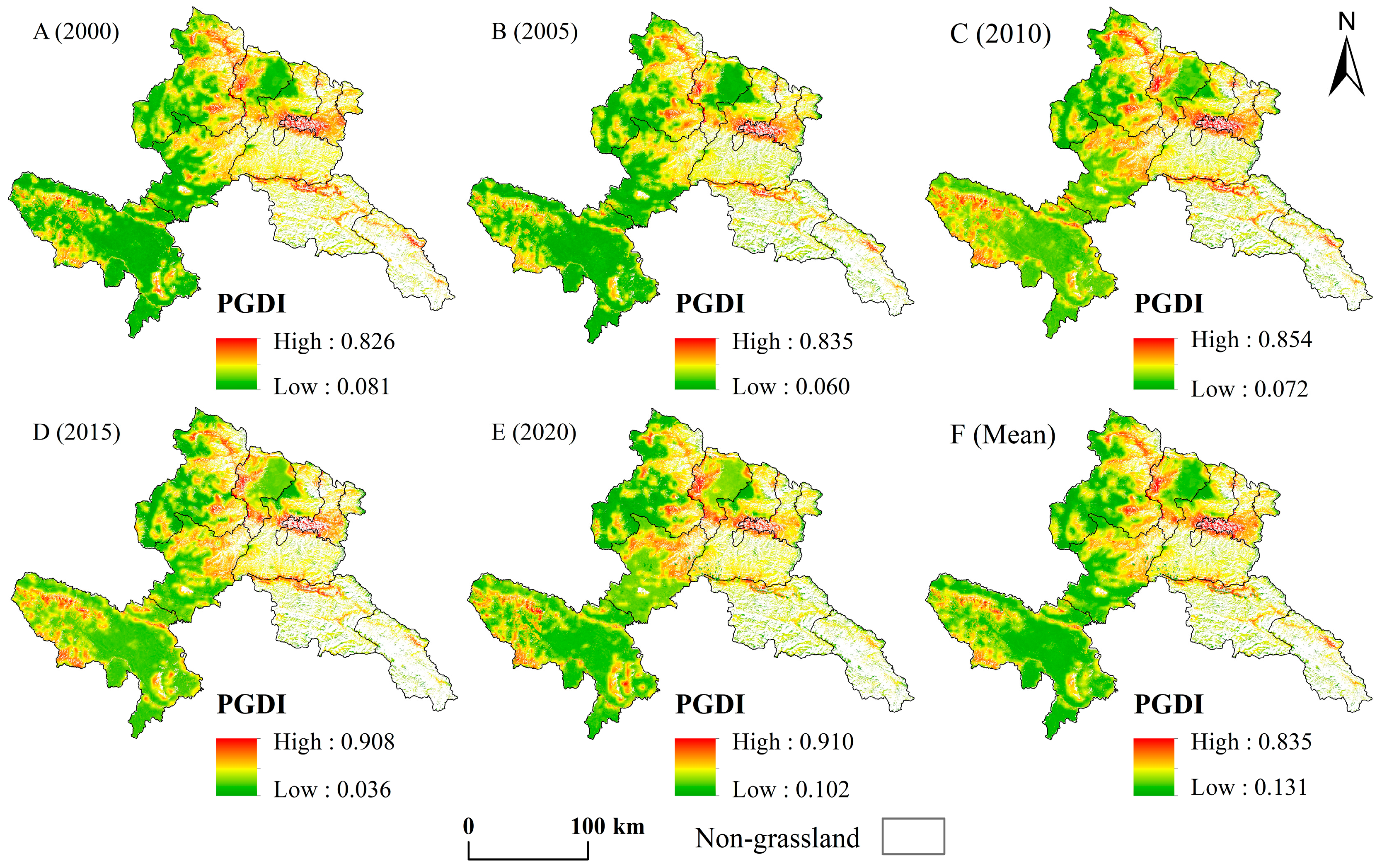
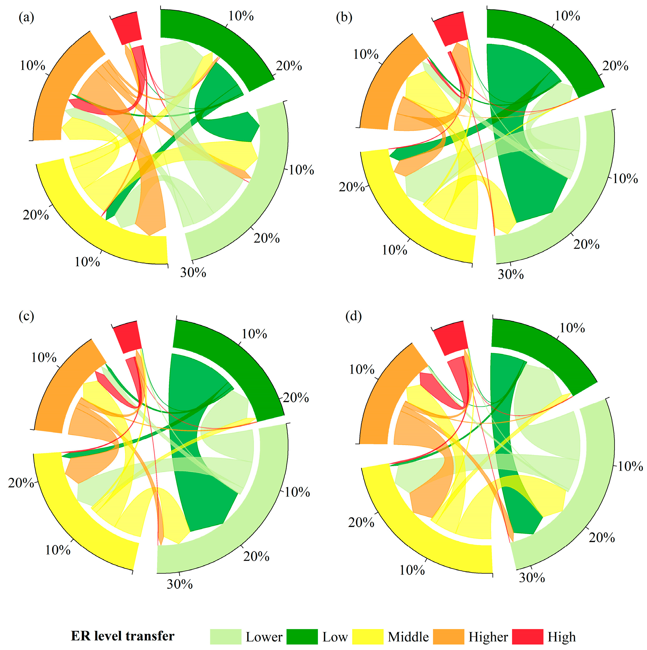
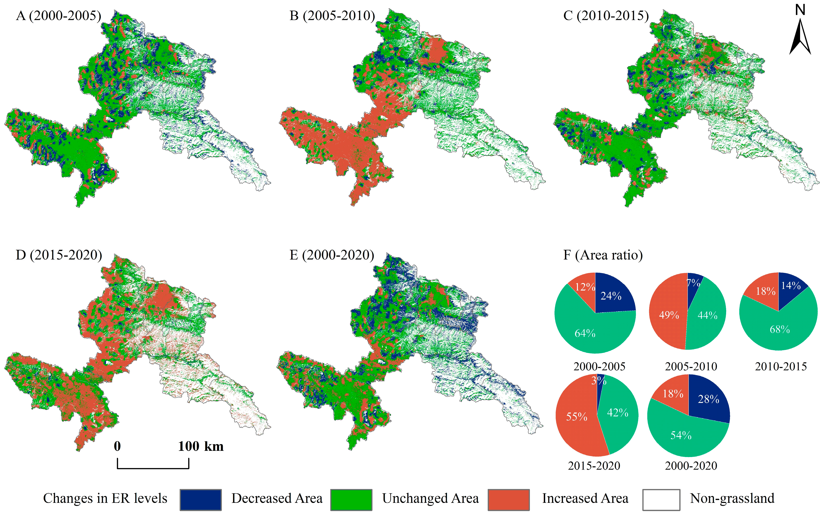
The spatial distribution of PGDI in the Gannan alpine grassland from 2000–2020 is shown in Figure 3. In this period, the PGDI of the Gannan alpine grassland ranged from 0.03 to 0.91, showing a trend of fluctuations. From a spatial perspective, the PGDI determined a spatial distribution pattern that was low in the northwest and high in the northeast. Specifically, the high-value areas were distributed in the northeast part of the Gannan alpine grassland, including the border of Diebu and Zhouqu Counties, the center of Lintan County, Eastern Xiahe County, and Western Hezuo. Meanwhile, the low-value areas were in Maqu County, Luqu County, and Eastern Xiahe County. The ER levels’ spatial distribution map in the alpine grasslands of Gannan Prefecture is shown in Figure 4. Generally, the ER levels were mainly in the mid-range and below. Medium- and low-risk areas accounted for a large proportion of the grasslands and were mainly distributed in Eastern Hezuo, Luqu County, and Southern Diebu County. The comprehensive ER transfer changes and the ER level changes in the Gannan alpine grassland are shown in Figure 5 and Figure 6. Specifically, the high-risk transfer area (22.09%) was smaller than the transfer-out area (28.41%), with the proportion demonstrating fluctuations in the form of an increase followed by a decrease. Overall, The ER changes across different periods remained relatively stable, with the unchanged areas predominating, accounting for 44% to 68% of the total area.

3.2. Spatiotemporal Characteristics of ESs

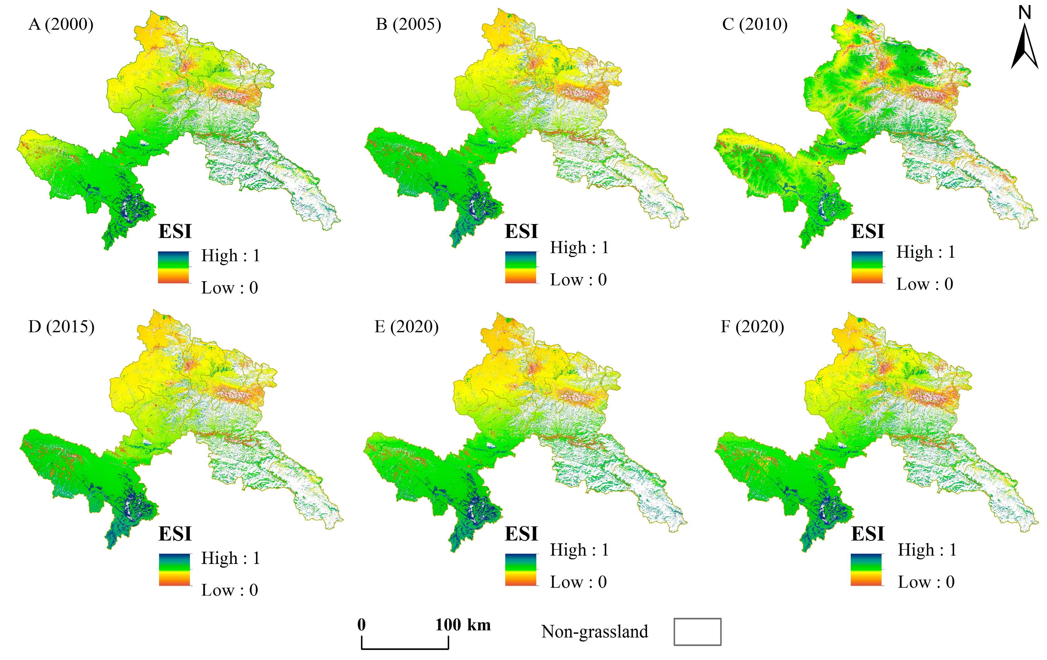
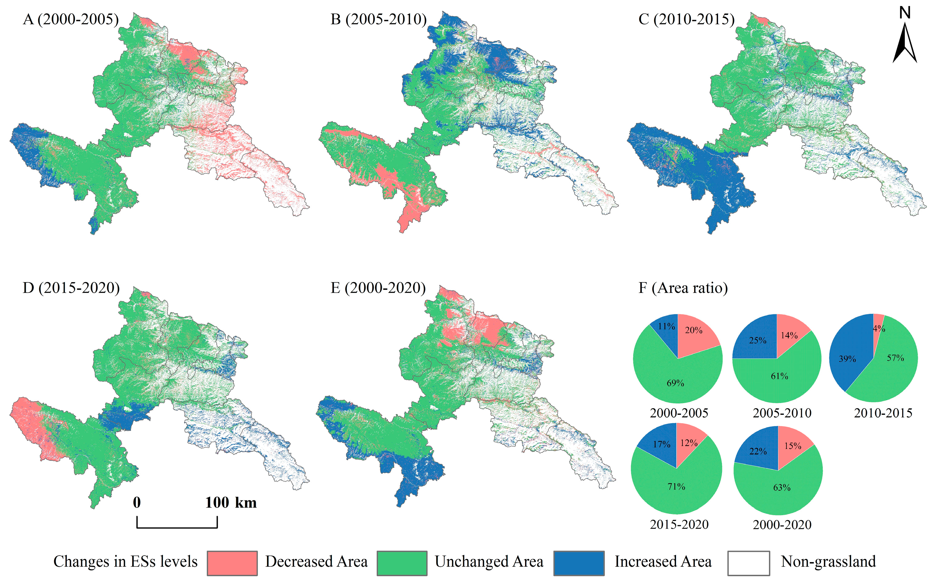
The spatiotemporal distribution of ESI in the alpine grassland in Gannan Prefecture from 2000–2020 is shown in Figure 7. The average ESI values were 0.42, 0.48, 0.43, 0.45, and 0.39 for 2000, 2005, 2010, 2015, and 2020, respectively, exhibiting an overall fluctuating trend with an initial increase followed by a decrease. The low-value areas were mainly concentrated in the west of Maqu County and Central Lintan County, with a small number being distributed across the border between Zhuoni and Diebu Counties, while the high-value areas were mainly in Southern Maqu County and the southwest of Luqu County. In the past 20 years, the ES level of the alpine grassland in Gannan has mainly been in the mid-range (Figure 8). The mid-range had the largest proportion (42%), showing a fluctuating trend of first increasing and then decreasing. It was mainly located in the northwest of the region, including West Maqu County, Luqu County, the southern part of Xiahe, and Hezuo. The comprehensive ESs transfer changes and ER level changes in the Gannan alpine grassland are shown in Figure 9 and Figure 10. In this period, the area transferred into high-service levels (18.70%) was smaller than the area transferred out (20.60%), and the proportion continued to decrease. The main transfers were to medium services (6.10%) and higher services (14.10%). In comparison, the ESs changes across different periods remained relatively stable (Figure 10), with the unchanged areas predominating, primarily distributed in the northwest of Gannan.

3.3. The Correlation between Comprehensive ER and ESs

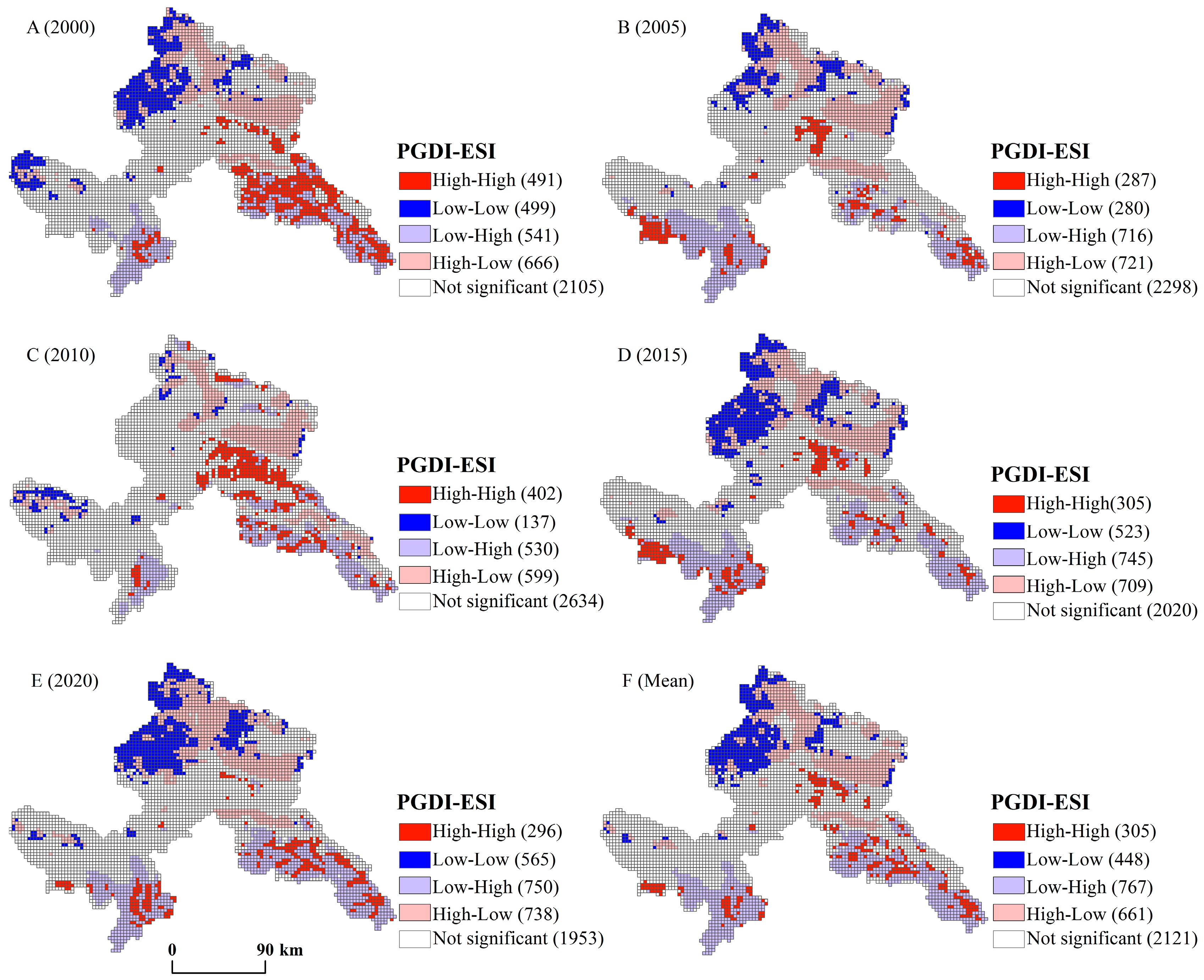
The Moran’s index values of the PGDI and ESI were −0.246, −0.429, −0.348, −0.320, and −0.285 for 2000–2020, and they passed the significance testing, indicating that they showed significant negative spatial correlations (Figure 11). In the time series, the spatial aggregation showed a trend of the Moran’s index of the PGDI and ESI first decreasing and then increasing, indicating that the spatial aggregation between PGDI and ESI increased and the spatial convergence was enhanced. Compared to the global Moran’s index, the local Moran’s index better reflected the spatial distribution of the ER and ESs. The local indicators of the spatial autocorrelation clustering map reflect the local spatial correlation characteristics that pass the significance test. As seen in Figure 12, the spatial clustering pattern was dominated by high–low and low–high, with the low–high clustering area concentrated in Diebu County, southwestern Zhouqu County, and southern Luqu County. This was mainly due to the low PGDI, the low probability of ER occurrence, and the high ESs index. In contrast, the high–low clustering area was sporadically distributed in Northern Xiahe, at the border of Xiahe and Hezuo, Lintan County, and the border between Zhuoni and Diebu Counties (Figure 12), and it mainly had high a PGDI but low ESI index, making the two negatively correlated.

3.4. Analysis of Driving Factors of Ecological Risk

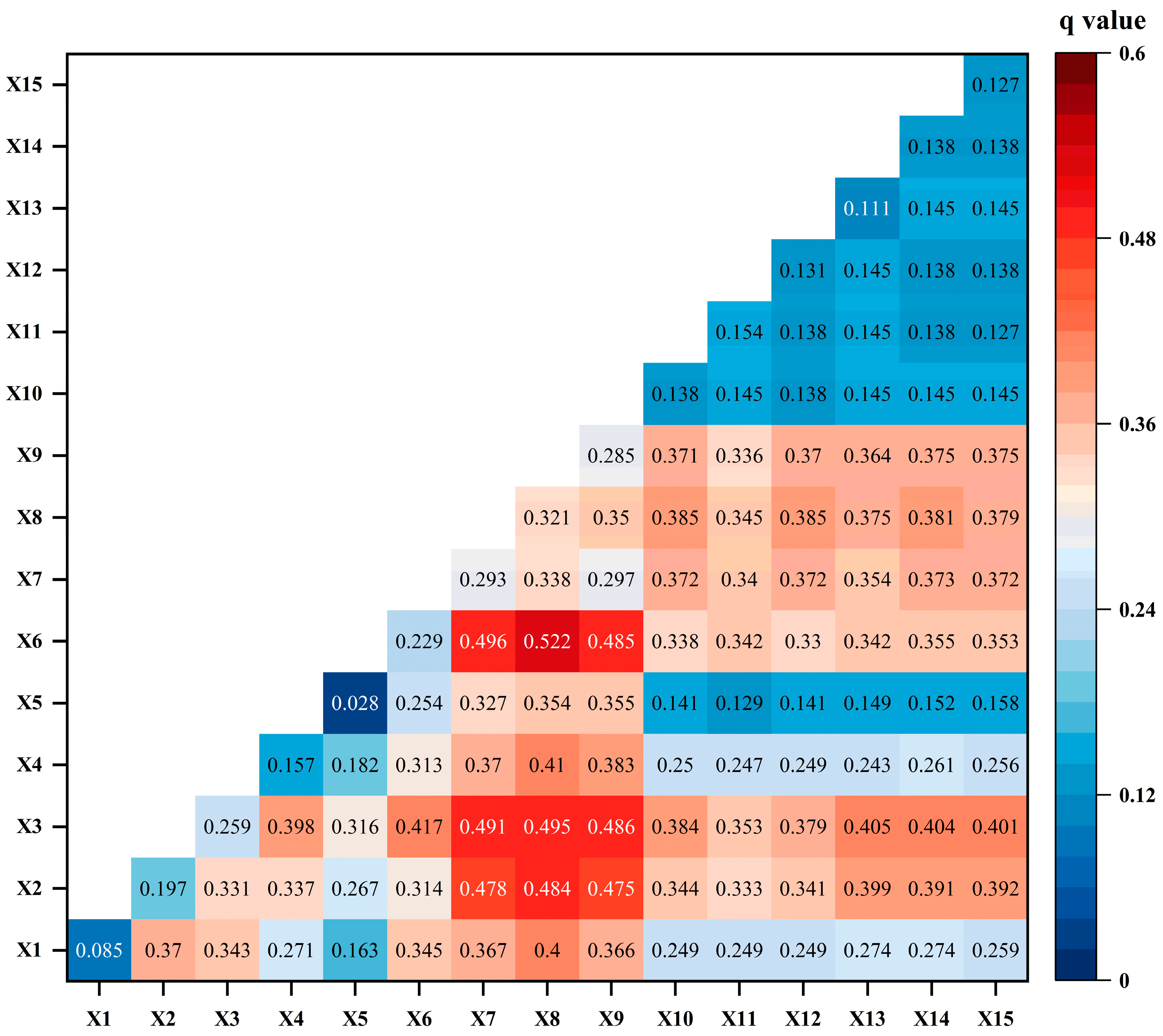
The drivers affecting the spatial heterogeneity of ER differed significantly (Figure 13), and the interaction among the drivers also varied greatly (Figure 14). The effect of each driving factor on ER passed the significance test (p < 0.05). Among these factors, the landscape was the primary dominant factor affecting ER, with q-values all greater than 0.28, followed by the temperature and the DEM, with q-values of 0.259 and 0.229, respectively. The influence of aspect was not significant. In addition, the interaction between the diversity index and NDVI had the greatest effect on ER (q-value = 0.522), followed by the interactions between precipitation and DEM with landscape index. However, the interaction between GDP per capita and aspect had the least impact on ER. In summary, the interaction between any two factors was greater than that of any single factor, indicating that the ER of the Gannan grassland was not caused by a single factor but by multiple drivers.

4. Discussion

4.1. A Comprehensive ERA of the Alpine Grassland Based on the PGDI

As a representation of ER, three aspects are taken into consideration in the newly proposed PGDI: grassland health status, landscape pattern changes, and human factors. Studies on regional-scale ER evaluation have primarily been based on land-use maps obtained from remote sensing images. For example, Peng et al. used Landsat images to create land cover maps of the Shengjin Lake Wetland in 2002, 2016, and 1986 [68]. After analyzing the data on land-use types and areas, the authors ultimately constructed a land-use ERA model. In a similar vein, Zhang et al. utilized the landscape pattern index for the computation of the ER index and analyzed the potential environmental influences of land use changes in China’s coastal cities from 1990–2015 [69]. Furthermore, in studies on grassland monitoring, grassland coverage and biomass have usually been used as indicators to evaluate whether grassland degradation damage has occurred, while other indicators have been easily ignored. However, under the influence of natural conditions such as climate, precipitation, and soil that are not conducive to the growth of grassland vegetation, as well as human factors such as overgrazing, grassland landscape patterns, edible forage proportions, and community structures, these indicators will change [70,71]. Therefore, only using indicators such as vegetation coverage or biomass to assess the damage status of grasslands does not yield a comprehensive understanding. This study considered three aspects: the health status of the grassland vegetation, changes in landscape patterns, and human factors. Moreover, it proposed a PGDI that integrated FVC, RSEI, LERI, and GLBI. Specifically, FVC is usually used to assess the extent of grassland vegetation cover, which can represent the basic health status of the grassland ecosystem; RSEI, integrates various remote sensing indicators, which can comprehensively reflect the quality of the ecological environment; LERI can be used to evaluate the impact of landscape pattern changes on ecosystem stability from the perspective of landscape ecology; and GLBI measures the balance between grassland and livestock, reflecting the carrying capacity and utilization status of the grassland. By integrating these indices into PGDI, this study was able to comprehensively and multidimensionally assess the ER of the Gannan alpine grasslands. Compared with traditional ERA, which directly uses the proportion of various landscape types as potential representations [72], the PDGI can more reasonably predict the possibility of ER occurrence. This method can systematically and comprehensively evaluate the ER of the Gannan grassland, which not only overcomes the limitations of traditional single-indicator methods but also provides a more scientific risk assessment through multi-angle and multi-level comprehensive analysis. It also provides an important theoretical basis and decision support for the protection and management of the Gannan alpine grassland.
In addition, this study systematically analyzed the spatiotemporal change characteristics of the PGDI’s three main factors (i.e., GRI, LERI, and GLBI) (Figure A4, Figure A5 and Figure A6). The GRI presented a spatial distribution pattern that was low in the southeast and high in the northwest (Figure A4). This pattern differed somewhat from that indicated by Huang et al. [73]. The main reason may be that our study focused on grasslands, while Huang et al. focused on the ecological resilience of multiple land use types. The LERI assessment not only analyzes the effects of ER on overall landscape fragmentation but also considers the extent of damage to specific risk receptors [13,74,75]. From 2000–2020, this assessment of the Gannan alpine grassland showed an increasing trend (Figure A5), which is similar to the results of the previous study [76]. This indicates that high-value areas were mainly distributed in areas with larger slopes and lower FVC, with more serious hydraulic erosion. The spatiotemporal distribution pattern of GLBI was high, which is consistent with the results of [77]. The high-value areas were mainly in these areas, with less grassland area and livestock, and, as the actual livestock-carrying capacity of the grassland was lower than the theoretical livestock-carrying capacity, there was sufficient grass for grazing (Figure A6). Unfortunately, due to the absence of township statistical yearbooks and the difficulties encountered in counting livestock in pasture areas, the actual livestock-carrying capacity in this study could only be approximated based on the year-end livestock stock in each county and city in Gannan Prefecture.
Overall, the grassland PGDI in Gannan Prefecture in the period of study showed an increasingly fluctuating trend of decreasing and then increasing (Figure 3). Its low-value areas were distributed in areas which had a relatively flat terrain, rich pasture resources, and good grassland vegetation growth, resulting in the ER being relatively low. The high-value areas were mainly distributed in the areas that experienced more concentrated rainfall, relatively serious soil erosion, and a higher frequency of geologic hazards. In addition, the PGDI was developed using the pixel scale, with a spatial resolution of 30 m, and it has good applicability in the study of ERA of alpine grasslands at the regional scale. Thus, the PGDI can generally effectively characterize the damage to and ER of the Gannan alpine grassland.

4.2. The Relationship between ESs and ER

Focusing on alpine natural grassland ecosystems in Gannan Prefecture, this study explored the dynamic relationship between ESs and ER. This study spatially visualized the total ESs of the alpine grassland in Gannan Prefecture based on ESI and analyzed the total ESs’ spatiotemporal distribution characteristics. The results indicated that the spatial distributions of the ESI had significant differences, exhibiting a spatial pattern of being low in the northwest and high in the southeast. When considering different service levels, the ESs level of Gannan alpine grassland were dominated by medium services, and from 2000–2020, the ESI of the alpine grassland in Gannan Prefecture showed a trend of first increasing and then decreasing, which might have been related to the intensification of human activities [45]. Moreover, our analysis showed a significant negative correlation between the PGDI and ESI (i.e., ESI gradually increased with decreasing PGDI), which further confirmed Dong et al.’s theory [78]. This finding provides a new perspective for understanding the spatial distribution patterns of ESs and ER and helps to identify key areas in ecosystem management. Our study shows that some areas with high ecosystem services are often accompanied by low ER, and vice versa. This negative correlation reveals the spatial complementarity of the two and supports the trade-off theory between ESs and ER. With the rapid development of human socio-economic activities, ERA is gradually becoming an important indicator to measure ESs [79]. However, incorporating ESs into regional ERA frameworks comes with certain challenges. First, ESs and ER are diverse and complex concepts, as there are multiple ESs and potential risks, and it is difficult to determine appropriate indicators and methods for effectively capturing this diversity and complexity. At the same time, the provision of an ES may be affected by multiple ecosystem processes and risk factors, which increases the complexity of analysis and simulation. Furthermore, ecosystem protection must focus on both supplying diverse ESs and maintaining high-level ecosystem health [80,81]. Therefore, there is a need to further improve the analytical framework and implement comprehensive assessments that can not only focus on the impacts on ESs but also maintain ecosystem health to ensure more effective ERA.

4.3. Driving Factors of ER

With the development of global climate change and rapid socio-economic growth, identifying the dominant factors influencing ER changes can provide valuable references for decision makers. In this study, the factor detection results indicate significant regional differences in the driving factors of ER changes in the alpine grassland of Gannan (Figure 13 and Figure 14). Generally, landscape and socio-economic factors have a greater impact on ER than natural environmental factors. Among landscape factors, the diversity index is the main influencing factor, highlighting the key influence of landscape structure on the ecosystem’s health in the Gannan region [82,83]. Natural factors, such as temperature, DEM, precipitation, slope, and NDVI are also significant, with average q-values greater than 0.2. This is likely due to the large spatial distribution differences in precipitation, temperature, and vegetation coverage in Gannan alpine grasslands. Shi et al. [84] noted that temperature and precipitation significantly impact vegetation on the Tibetan Plateau, which aligns with our findings that climatic conditions in alpine regions generally affect ER [18,85]. Furthermore, our results indicate that DEM and slope contribute significantly to ER under the unique terrain conditions of Gannan Prefecture. In addition, precipitation is concentrated in the southeastern part of the Gannan alpine grassland, leading to frequent geological disasters and affecting human production and life. It is noteworthy that land reclamation rate, grazing pressure, GDP per capita, and fertilizer usage have a significant impact on the ER of Gannan alpine grassland, with q-values all greater than 0.13. This change is likely due to rapid socio-economic development, increasing ecological pressure and affecting grassland health. Our study is consistent with Yang et al. [16], who showed that increases in socio-economic activities heighten ER, particularly the pressure on ecosystems caused by land use changes [86,87]. Specifically, increased land reclamation often converts grassland to farmland or other uses, leading to the destruction of natural ecosystems. Similarly, overgrazing can cause grassland degradation and may lead to sandification and desertification [88]. Although a higher GDP per capita indicates improved economic development, it also leads to increased resource consumption and pollution, such as increased fertilizer usage. Excessive fertilizer use directly affects soil and water quality. Therefore, comprehensive measures need to mitigate the negative impact of these socio-economic factors on ER. For example, rational land use planning, controlling land reclamation and overgrazing, promoting sustainable agriculture and ecological farming technologies, and reducing the use of chemical fertilizers and pesticides are essential. Additionally, strengthening the implementation of environmental protection policies and promoting sustainable social and economic development are crucial.

4.4. Limitations and Prospects

Although our study enhances the ecological indications of the evaluation results, there are still some shortcomings that need to be addressed. First, three ESs were selected for evaluation, and this study relied on the natural ecological environment of Gannan, which is somewhat subjective. Second, although the InVEST model was employed for the computation of HQ, WY, and SC services, there is still some uncertainty in the estimation results. For example, when evaluating the WY, the low spatial resolution of the images of annual potential plant available water content, evapotranspiration, and root depth as well as the influence of temporal constraints could have led to unclear or incomplete data. Third, a large number of high-precision observations and actual data were required for the InVEST model, but the study area was relatively complex and had fewer measured data. Fourth, when evaluating the individual ESs, the parameter values were obtained using empirical methods or similar areas, which could have led to subjective errors, and the evaluation results were not further quantitatively verified. Lastly, the existence of synergistic and trade-off relationships between ESs may have had an impact on the ESI, which could have subsequently affected the results. Therefore, subsequent research needs to consider the functional supply and demand of ESs as well as the synergies and trade-offs between ESs.
In constructing the PGDI for this study, its feasibility in practical applications was prioritized. Therefore, the data sources used in this paper were open source and had global coverage, such as WorldPop population data, including the grassland health status, landscape pattern changes, and human factors in the PGDI. Additionally, the ERA also had a certain degree of subjectivity. Therefore, the PGDI indicator system can be further optimized. In addition, the PGDI was used to characterize ERs, and this study only analyzed the ER changes every five years, which made it difficult to summarize the interannual changes in the comprehensive ER of Gannan Prefecture’s grassland. In subsequent studies, high-resolution and long-time-series grass vegetation mapping can be used to transform the grass evolution trend into an indicator to enrich the construction of the PGDI so that it can be used to characterize the degree of past damage and the risk of future damage to grasslands. Moreover, the present study only focused on alpine grassland, so whether the findings are generalizable to the ERA of other grassland types remains to be further verified. Therefore, future studies can extend the PGDI’s application to other grassland types or different land-use scenarios and provide more information regarding its direct application to grassland and regional ecological environmental protection. In addition, since the influencing factors of ER are complex and diverse, this study quantified the influencing factors from the perspective of spatial differentiation, but how to comprehensively analyze the coupling effects between multiple factors is a difficult problem that needs to be solved in the current study of the driving force impact on ER. Future work should explore the impact of natural and socio-economic factors on ER from multiple geospatial data sources to provide a deeper understanding of the driving mechanisms of ER changes in Gannan alpine grasslands.

5. Conclusions

This study proposed a new comprehensive ERA framework and PGDI based on GRI, LERI, and GLBI, and it analyzed the ER in Gannan Prefecture and its spatiotemporal distribution patterns for 2000, 2005, 2010, 2015, and 2020. It also examined the spatiotemporal distribution of ESs in Gannan Prefecture’s alpine grassland and investigated the correlation and response relationship between the two. Finally, the geographic detector model was introduced to explore the driving factors affecting ER. Overall, the PGDI in Gannan Prefecture showed an increasing trend from 2000–2020, and the ER continued to increase. In addition, the ESI of the alpine grassland in Gannan Prefecture showed a fluctuating trend of increasing and then decreasing, with the average value decreasing from 0.43 to 0.39 during the period of study and a large loss of ESs. Moreover, there was a significant negative spatial autocorrelation between the PGDI and ESI, with obvious spatial aggregation.
Based on the Geodetector analysis, landscape and socio-economic factors have a greater impact on ER than natural factors. Moreover, this study revealed that the interaction between any driving factors has a more significant impact than a single driving factor. Notably, the interaction between the landscape index and NDVI had the highest q-value. Future efforts should focus on integrating fragmented landscapes and optimizing landscape structures, particularly in areas with high NDVI and grassland coverage. Landscape risk source management planning should aim to minimize human interference, and regional planning should prioritize increasing the construction of ecological land. Furthermore, it is crucial to rationally plan land use; strictly control the conversion of grassland to other land use types, reclamation, and overgrazing; promote sustainable and ecological agriculture technologies; reduce the use of chemical fertilizers and pesticides; and strengthen the implementation of environmental protection policies. In summary, the proposed new assessment framework of ER in alpine grasslands has good applicability and potential, and it will develop a significance theoretical basis for the protection of the grassland ecosystems and scientific management in Gannan Prefecture.

Author Contributions

Z.M.: methodology, data curation, writing. J.G.: conceptualization, methodology. T.L.: resources, methodology. Z.H.: methodology, software. S.F.: resources, visualization. X.Z.: resources, visualization. D.Z.: supervision. All authors have read and agreed to the published version of the manuscript.

Funding

This study was supported by the Major Science and Technology Projects of Gansu Province (21ZD4FA020) and the National Key Research and Development Program of China project (2021YFD1300504).

Data Availability Statement

The raw data supporting the conclusions of this article will be made available by the authors on request.

Acknowledgments

We acknowledge the reviewers and academic editors for their positive and constructive comments and suggestions. We are grateful to the assistant editor and English editor for processing our manuscript efficiently.

Conflicts of Interest

All co-authors declare that there are no conflicts of interest.

Appendix A

Appendix A.1. Calculation Methods and Results for the Three Ecosystem Services

To evaluate the ecosystem services (ESs) of Gannan Prefecture, we examined three general evolution indicators: water yield (WY), soil conservation (SC), and habitat quantity (HQ). The calculations were made according to relevant research methods and the parameter settings in Gannan Prefecture.
(1)
HQ
HQ refers to an ecosystem’s ability to provide suitable conditions for the continued survival of populations and individuals [89]. InVEST’s HQ module relies on threat-source and data land-use data, and it is calculated based on the response of distinct habitats to threat sources [73]. The calculation formula is as follows:
H Q = H j 1 D x j z D x j z + k z
D x y = r = 1 R y = 1 Y r W r r = 1 R W r r y i r x y β x S j r
where HQ is the habitat quality value, Dxj is the habitat degradation degree at grid x of land-use type j, Hj is the habitat adaptability of land-use type j, ry is the intensity of the threat factor r, y is the grid number of the threat factor r, wr is the weight of threat factor r (Table A1), Sjr is the relative sensitivity degree of land-use type j to threat factors r, and βx is the level of accessibility of grid x (Table A2).
Table A1. Parameters for threat factors.
Threat FactorsLongest Threat DistanceWeightSpatial Decay Type
National highway
and provincial highway
2.5 km0.6Linear decay
County road0.5 km0.5Linear decay
Housing estate2.5 km0.4Exponential decay
Towns6.0 km0.8Exponential decay
Population density3.5 km0.3Exponential decay
Unused land1.5 km0.6Exponential decay
Table A2. Land-use type sensitivity and adaptability to threat factors.
Land-Use TypeHabitat AdaptabilityNational Road and Provincal RoadCounty RoadHousing EstateTownsPopulation DensityCultivated Land
Cultivated land0.30.50.60.40.50.80.0
Grassland0.80.70.50.20.30.50.5
Forest land1.00.90.70.50.60.70.3
Water areas0.90.750.650.70.80.50.1
Wetland1.00.80.60.90.70.50.1
Construction land0.00.00.00.00.00.850.0
Unused land0.010.20.20.10.10.30.1
The spatiotemporal distribution of the HQ from 2000–2020 is shown in Figure A1. Specifically, areas with a higher habitat quality were mainly distributed on the border between Hezuo and Zhuoni Counties and in the northeast of Hezuo, the southwest of Luqu County, and the south of Maqu County. The areas with a lower habitat quality were distributed in Lintan County, around the center of Hezuo, in Northern Diebu and in the alpine areas of the western pastoral areas. This pattern emerged because areas with high human activity intensity were close to towns and cities, and denser transportation networks are more threatened.
Figure A1. The spatiotemporal distribution of habitat quantity in Gannan Prefecture.
Remotesensing 16 02242 g0a1
(2)
WY
WY service is closely related to humans and refers to the amount of water produced per unit area in a certain period [90]. The InVEST WY model runs on a raster map and determines the regional ecosystem’s water production [91] by computing the difference between regional moisture input and output. The calculation formula is as follows:
W Y = 1 A E T x j P x × P x
A E T X P x = 1 + ω x + R x j 1 + ω x R x j + 1 / R x j
ω x = Z A W C X P x
R x j = k × E T 0 P x
where WY is the water yield value (mm), AETxj is the actual annual evapotranspiration at grid x of land-use type j, wx is the porous ratio, Rx is the potential evapotranspiration to precipitation ratio, and ET0 is the potential evapotranspiration. For land-use types with vegetation, the evapotranspiration part of the water balance AETx/Px was developed based on the Budyko curve [91], and the annual rainfall was determined based on the daily rainfall data of meteorological stations. The MOD16A3 product was selected for annual potential evaporation, and the watershed map was based on digital elevation model (DEM) data and extracted using the hydrological analysis model tool in ArcGIS10.2. A total of 60 sub-watersheds were generated in this study. We also referred to the relevant literature and set z as 9.433 [92]. In addition, referring to similar studies [93], the AWCx was calculated using the following equations:
A W C x = m i n s o i l _ d e p t h , r o o t _ d e p t h × P W A C
P W A C = 54.509 0.132 × S A N 0.003 × S A N 2 0.055 × S I L 0.006 × S I L 2 0.738 × C L A + 0.007 × C L A 2 2.688 × O M + 0.501 × O M 2 × 100 %
where root_depth is the depth of plant roots and soil_depth is the depth of the soil (mm) obtained from the soil data sets (Table A3). PAWC is the amount of water available to plants, and OM, SIL, SAN, and CLA represent the organic matter percentage (%), silt percentage (%), soil sand percentage (%), and clay percentage (%), respectively, where the OM content is equal to the organic carbon content (%) multiplied by 1.724. In addition, the WY model requires the biophysical coefficients of land-use types to be input (see Table A3 for details).
Table A3. Biophysical parameters of different land-use types.
Land-Use TypeLucodeCoefficient of Vegetation Transpiration kRoot Depth (mm)LULC_veg
Cultivated land10.653001
Grassland20.755001
Forest land30.765001
Water areas4100
Wetland50.73001
Construction land60.210
Unused land70.3100
Lucode is the land use type code, and LULC_veg is the mark that distinguishes bare land and vegetated land.
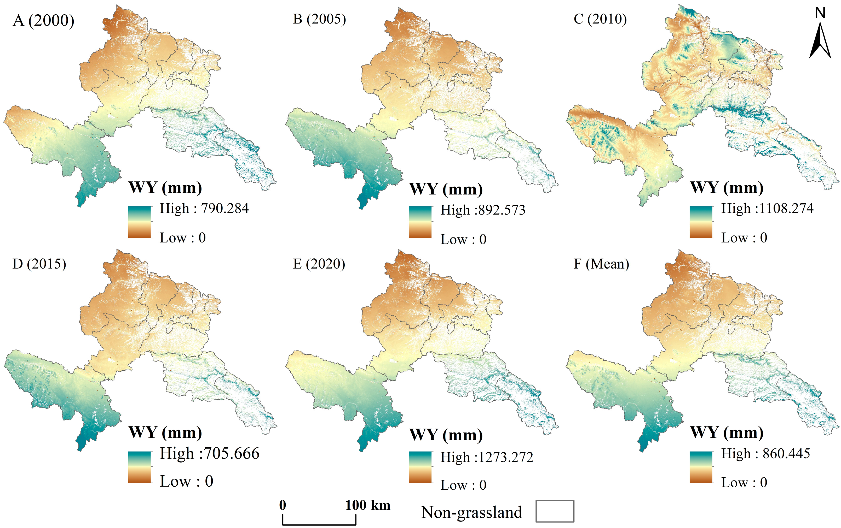
The spatiotemporal distribution of the WY is shown in Figure A2. In 2000, 2005, 2010, 2015, and 2020, the average annual water production was 386.3 mm, 551.9 mm, 545.9 mm, 381.0 mm, and 639.1 mm, respectively. Overall, the dry climate, limited rainfall, and other factors led to lower water production in the north, while high values of WY supply services were mainly distributed in the Southern Maqu Counties, Eastern Diebu, and Northeastern Zhouqu.
Figure A2. The spatiotemporal distribution of water yield in Gannan Prefecture.
Remotesensing 16 02242 g0a2
(3)
SC
SC is the process of preventing soil erosion and retaining sediment, which has a positive impact on land productivity and many other ESs. SC measures the variation between potential soil erosion versus actual soil erosion rates [94]. The formula is as follows:
S C x = R K L S x U S L E x
R K L S X = R x · K x · L S x
U S L E X = R x · K x · L S x · C x · P x
where R K L S X is the potential soil loss, C x is the vegetation cover factor, U S L E x is the actual amount of soil erosion, P x is the soil conservation measures factor, and L S x is the factor of slope length and slope gradient. The DEM data were imported into the InVEST model using the fill-and-cut process in ArcGIS 10.2 to calculate the slope gradient and slope length, and C and P were constructed by reviewing the relevant literature [95]. The results for the area were used to construct a coefficient table (Table A4), and the R-factor was estimated using Wishmeier’s monthly scale estimation method as follows:
R = i = 1 12 1.735 × 10 1.5 l g P i 2 P 0.8188
where P i is the soil erosion factor of the average rainfall for the month, and K reflects the soil properties that are sensitivity to erosion. This study refers to the following empirical formula [96]:
K E R I C = 0.2 + 0.3 e 0.0256 S A N 1 S I L 100 × S I L C L A + S I L 0.3 × 1.0 0.25 C C + e 3.72 2.95 C × 1.0 0.7 S N I S N I + e 22.9 S N I 5.51
K = 0.01383 + 0.51575 K E P I C × 0.1317
where SIL, SAN, C, and CLA represent the soil silt percentage (%), sand percentage (%), soil organic carbon in the surface layer (0–30 cm) percentage (%), and clay percentage (%), respectively, and the SNI is calculated based on the relationship 1–SAN/100.
Table A4. Soil conservation measure factors of various land-use types.
Land-Use TypesCode of Land-Use Typesp Factor Value
Cultivated land 0.20.15
Grassland0.31
Forest land0.051
Water areas00
Wetland0.051
Construction land01
Unused land11
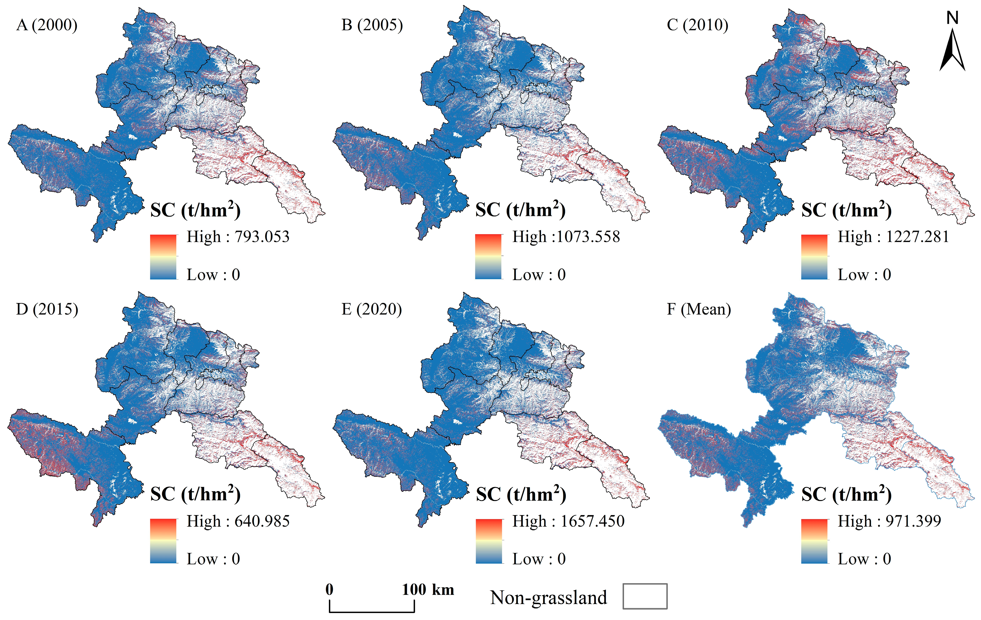
The spatiotemporal distribution of SC from 2000–2020 is shown in Figure A3. The total SC capacities of the Gannan alpine grassland were 5.58 × 10⁸ t, 3.88 × 10⁸ t, 16.99 × 10⁸ t, 4.89 × 10⁸ t, and 9.72 × 10⁸ t in 2000, 2005, 2010, 2015, and 2020, respectively, showing an increasing, decreasing, and increasing trend. The entire region remained elevated. The low-value areas were mainly distributed in Maqu, Luqu (near Gahai), and Xiahe Counties, as well as Hezuo, and the high-value areas were mainly distributed in grasslands in Zhouqu, Diebu, and Zhuoni Counties.
Figure A3. The spatiotemporal distribution of soil conservation in Gannan Prefecture.
Remotesensing 16 02242 g0a3

Appendix A.2. Calculation Results for the Three Indicators of the PGDI

(1)
Grassland resilience index
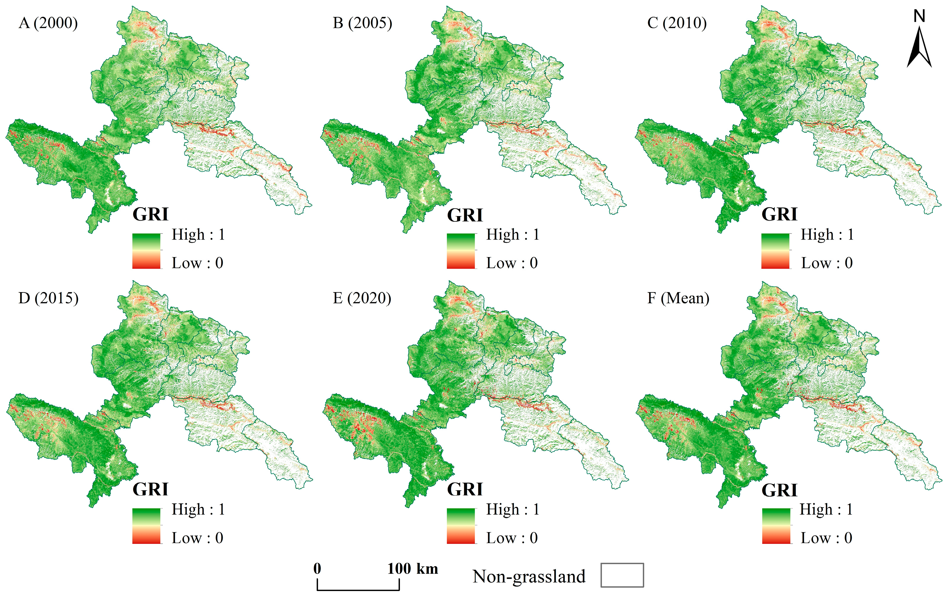
The spatiotemporal distribution of the grassland resilience index (GRI) from 2000–2020 is shown in Figure A4. In 2000, 2005, 2010, 2015, and 2020, the annual average values of the GRI of Gannan Prefecture’s alpine grassland were 0.705, 0.710, 0.713, 0.745, and 0.772, respectively, which demonstrated a general increasing trend. The low-value areas were mainly distributed in Northern Xiahe County, the border between Diebu and Zhuoni Counties, and Western Maqu County. High-GRI-value areas were mainly distributed in Maqu, Luqu, Western Xiahe Counties, most of the southeastern part of Hezuo, and the border between Hezuo City and Zhuoni County.
Figure A4. The spatiotemporal distribution of the grassland resilience index in Gannan Prefecture.
Remotesensing 16 02242 g0a4
(2)
Landscape ecological risk index
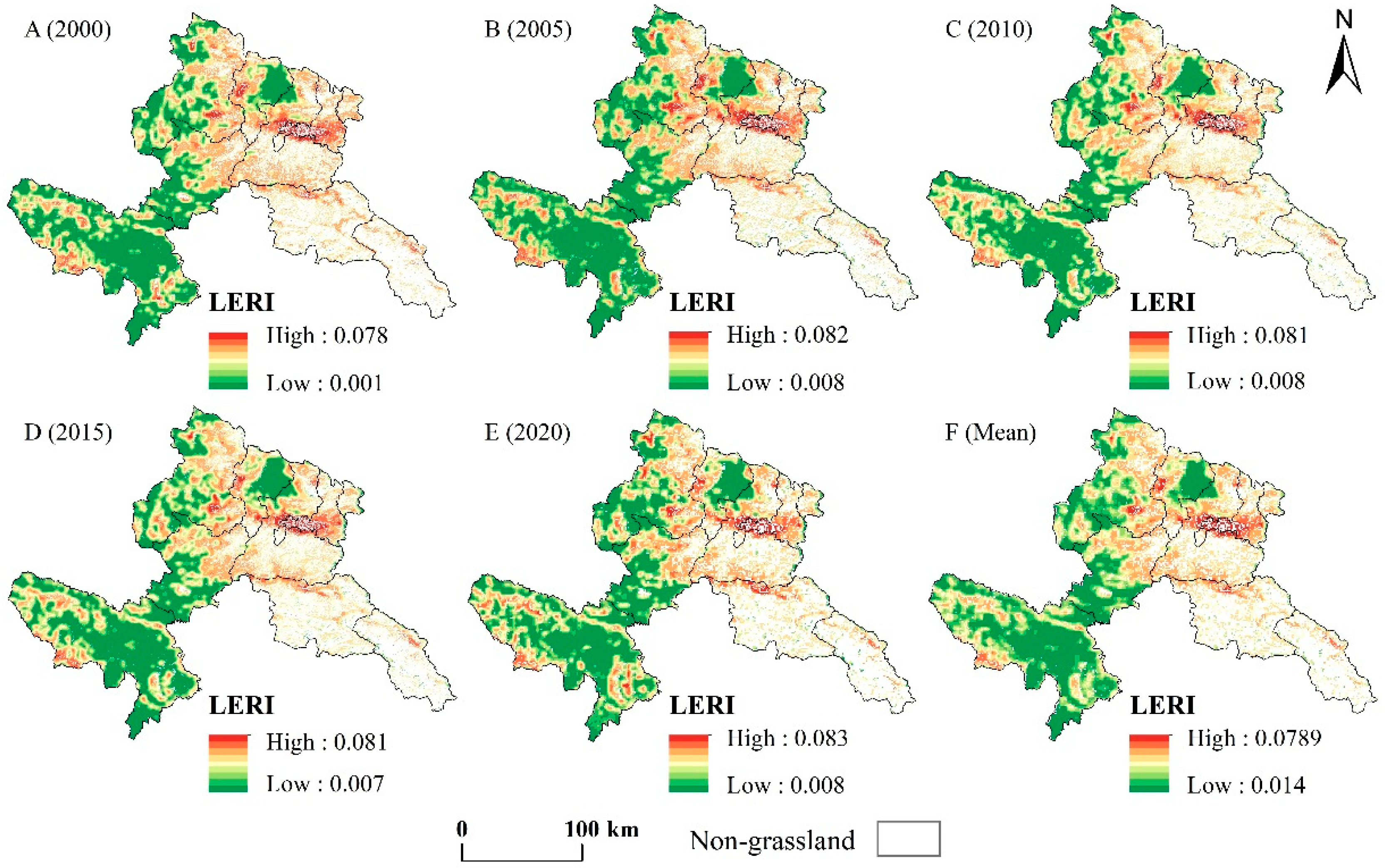
The spatiotemporal distribution of the landscape ecological risk index (LERI) in 2000, 2005, 2010, 2015, and 2020 is shown in Figure A5, for which the annual average values were 0.036, 0.036, 0.037, 0.036, and 0.037, respectively. The low-value areas were mainly distributed in the southwest of Xiahe County, Luqu County, Northern Zhuoni County, and most of Maqu County, where the vegetation cover was high. Meanwhile, the high-value areas were mainly distributed in Northwest Maqu County, the border between Diebu and Zhuoni Counties, central Hezuo-Lintan, and the south of Xiahe County. These ecosystem services were lost due to the large gradient, low vegetation cover, and relatively serious hydraulic erosion, resulting in excessive landscape ER of the grassland. The service loss was large, leading to the landscape ER of the grassland being higher.
Figure A5. Spatiotemporal distribution of landscape ecological risk index in Gannan Prefecture.
Remotesensing 16 02242 g0a5
(3)
Grass–livestock balance index
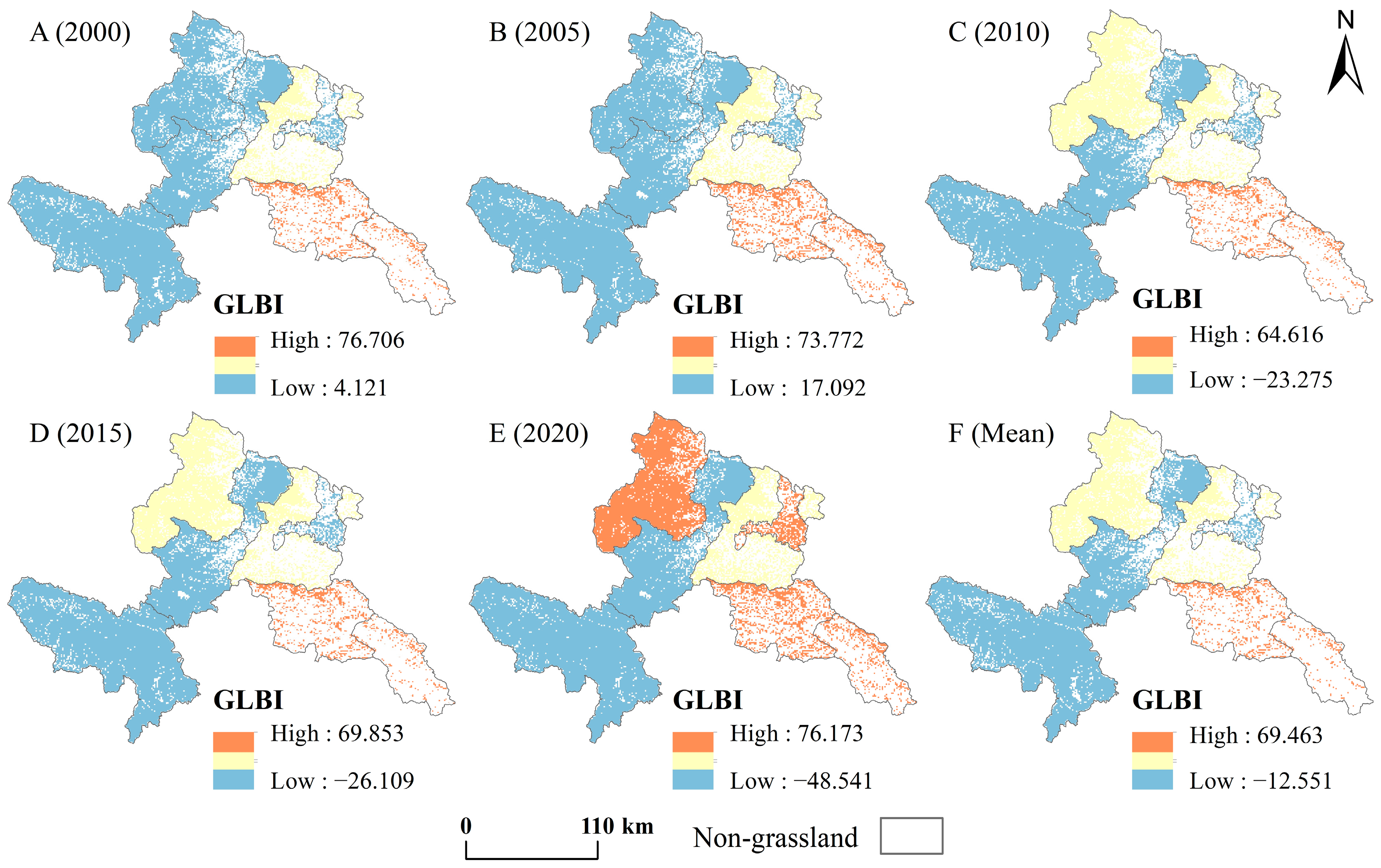
The spatiotemporal distributions of the grass–livestock balance index (GLBI) in 2000, 2005, 2010, 2015, and 2020 are shown in Figure A6, for which the annual averages were 23.324, 29.166, 1.267, 1.974, and 0.789, respectively, in Gannan Prefecture’s alpine grasslands. This shows an overall fluctuation trend of first rising and then falling. The low-value areas were distributed in areas with large grassland areas such as Hezuo as well as Xiahe, Luqu, and Maqu Counties. The high-value areas were mainly distributed in Zhuoni County, Diebu County, and most areas of Zhouqu County, which had less livestock than the theoretical livestock-carrying capacity and less grassland area, meaning that the area can support grazing.
Figure A6. Spatiotemporal distribution of grass–livestock balance index in Gannan.
Remotesensing 16 02242 g0a6
Table A5. Interaction between two explanatory variables and their interactive impacts.
Interaction RelationshipInteraction Type
q(X1∩X2) < Min(q(X1), q(X2))Nonlinear-weaken: Impacts of single variables are nonlinearly weakened by the interaction between two variables.
Min(q(X1), q(X2)) < q(X1∩X2) < Max(q(X1), q(X2))Uni-variable weaken: Impacts of single variables are uni-variable weakened by the interaction.
q(X1∩X2) > Max(q(X1), q(X2))Bi-variable enhance: Impact of single variables are bi-variable enhanced by the interaction.
q(X1∩X2) = q(X1) + q(X2)Independent: Impacts of variables are independent.
q(X1∩X2) > q(X1) + q(X2)Nonlinear-enhance: Impacts of variables are nonlinearly enhanced.

References

  1. Bengtsson, J.; Bullock, J.M.; Egoh, B.; Everson, C.; Everson, T.; O’Connor, T.; O’Farrell, P.J.; Smith, H.G.; Lindborg, R. Grasslands—More Important for Ecosystem Services than You Might Think. Ecosphere 2019, 10, e02582. [Google Scholar] [CrossRef]
  2. Lieth, H. Patterns of Primary Production in the Biosphere; Dowden, Hutchinson & Ross: Stroudsburg, PA, USA, 1978. [Google Scholar]
  3. Stevens, N.; Bond, W.; Feurdean, A.; Lehmann, C.E.R. Grassy Ecosystems in the Anthropocene. Annu. Rev. Environ. Resour. 2022, 47, 261–289. [Google Scholar] [CrossRef]
  4. Dong, S.; Shang, Z.; Gao, J.; Boone, R.B. Enhancing Sustainability of Grassland Ecosystems through Ecological Restoration and Grazing Management in an Era of Climate Change on Qinghai-Tibetan Plateau. Agric. Ecosyst. Environ. 2020, 287, 106684. [Google Scholar] [CrossRef]
  5. Zhang, G.; Zhang, Y.; Dong, J.; Xiao, X. Green-up Dates in the Tibetan Plateau Have Continuously Advanced from 1982 to 2011. Proc. Natl. Acad. Sci. USA 2013, 110, 4309–4314. [Google Scholar] [CrossRef] [PubMed]
  6. Deng, X.; Gibson, J.; Wang, P. Quantitative Measurements of the Interaction between Net Primary Productivity and Livestock Production in Qinghai Province Based on Data Fusion Technique. J. Clean. Prod. 2017, 142, 758–766. [Google Scholar] [CrossRef]
  7. Harrison, M.T.; Cullen, B.R.; Rawnsley, R.P. Modelling the Sensitivity of Agricultural Systems to Climate Change and Extreme Climatic Events. Agric. Syst. 2016, 148, 135–148. [Google Scholar] [CrossRef]
  8. Wu, P.; Zhan, W.; Cheng, N.; Yang, H.; Wu, Y. A Framework to Calculate Annual Landscape Ecological Risk Index Based on Land Use/Land Cover Changes: A Case Study on Shengjin Lake Wetland. IEEE J. Sel. Top. Appl. Earth Obs. Remote Sens. 2021, 14, 11926–11935. [Google Scholar] [CrossRef]
  9. Xu, D. Ecological Risk Assessment and Forecast of Gannan Rangeland. Ph.D. Thesis, Lanzhou University, Lanzhou, China, 2011. (In Chinese). [Google Scholar]
  10. Zhao, Y. Alpine Grassland Ecological Security Assessment for the Headwaters of the Yellow River, China. Ph.D. Thesis, Lanzhou University, Lanzhou, China, 2021. (In Chinese). [Google Scholar]
  11. Estoque, R.C.; Murayama, Y. Measuring Sustainability Based upon Various Perspectives: A Case Study of a Hill Station in Southeast Asia. AMBIO 2014, 43, 943–956. [Google Scholar] [CrossRef] [PubMed]
  12. Norton, S.B.; Rodier, D.J.; Van Der Schalie, W.H.; Wood, W.P.; Slimak, M.W.; Gentile, J.H. A Framework for Ecological Risk Assessment at the EPA. Environ. Toxicol. Chem. 1992, 11, 1663–1672. [Google Scholar] [CrossRef]
  13. Jin, X.; Jin, Y.; Mao, X. Ecological Risk Assessment of Cities on the Tibetan Plateau Based on Land Use/Land Cover Changes—Case Study of Delingha City. Ecol. Indic. 2019, 101, 185–191. [Google Scholar] [CrossRef]
  14. Walker, R.; Landis, W.; Brown, P. Developing a Regional Ecological Risk Assessment: A Case Study of a Tasmanian Agricultural Catchment. Hum. Ecol. Risk Assess. Int. J. 2001, 7, 417–439. [Google Scholar] [CrossRef]
  15. Wu, J.; Zhu, Q.; Qiao, N.; Wang, Z.; Sha, W.; Luo, K.; Wang, H.; Feng, Z. Ecological Risk Assessment of Coal Mine Area Based on “Source-Sink” Landscape Theory: A Case Study of Pingshuo Mining Area. J. Clean. Prod. 2021, 295, 126371. [Google Scholar] [CrossRef]
  16. Yang, Y.; Chen, J.; Lan, Y.; Zhou, G.; You, H.; Han, X.; Wang, Y.; Shi, X. Landscape Pattern and Ecological Risk Assessment in Guangxi Based on Land Use Change. Int. J. Environ. Res. Public. Health 2022, 19, 1595. [Google Scholar] [CrossRef]
  17. Lemly, A.D. Risk Assessment as an Environmental Management Tool: Considerations for Freshwater Wetlands. Environ. Manag. 1997, 21, 343–358. [Google Scholar] [CrossRef]
  18. Hou, M.; Ge, J.; Gao, J.; Meng, B.; Li, Y.; Yin, J.; Liu, J.; Feng, Q.; Liang, T. Ecological Risk Assessment and Impact Factor Analysis of Alpine Wetland Ecosystem Based on LUCC and Boosted Regression Tree on the Zoige Plateau, China. Remote Sens. 2020, 12, 368. [Google Scholar] [CrossRef]
  19. Bao, K.; Liu, J.; You, X.; Shi, X.; Meng, B. A New Comprehensive Ecological Risk Index for Risk Assessment on Luanhe River, China. Environ. Geochem. Health 2018, 40, 1965–1978. [Google Scholar] [CrossRef]
  20. Li, Z.; Jiang, W.; Wang, W.; Chen, Z.; Ling, Z.; Lv, J. Ecological Risk Assessment of the Wetlands in Beijing-Tianjin-Hebei Urban Agglomeration. Ecol. Indic. 2020, 117, 106677. [Google Scholar] [CrossRef]
  21. Yue, D.; Zeng, J.; Yang, C.; Zou, M.; Li, K.; Chen, G.; Guo, J.; Xu, X.; Meng, X. Ecological Risk Assessment of the Gannan Plateau, Northeastern Tibetan Plateau. J. Mt. Sci. 2018, 15, 1254–1267. [Google Scholar] [CrossRef]
  22. Cai, D. Ecosystem Risk Assessment of Alpine Grassland: A Case of the Gannan Region. Ph.D. Thesis, Lanzhou University, Lanzhou, China, 2019. (In Chinese). [Google Scholar]
  23. Chen, S.; Chen, B.; Fath, B.D. Ecological Risk Assessment on the System Scale: A Review of State-of-the-Art Models and Future Perspectives. Ecol. Model. 2013, 250, 25–33. [Google Scholar] [CrossRef]
  24. Peng, J.; Liu, Y.; Liu, Z.; Yang, Y. Mapping Spatial Non-Stationarity of Human-Natural Factors Associated with Agricultural Landscape Multifunctionality in Beijing–Tianjin–Hebei Region, China. Agric. Ecosyst. Environ. 2017, 246, 221–233. [Google Scholar] [CrossRef]
  25. Wu, X.; Wang, S.; Fu, B.; Liu, Y.; Zhu, Y. Land Use Optimization Based on Ecosystem Service Assessment: A Case Study in the Yanhe Watershed. Land Use Policy 2018, 72, 303–312. [Google Scholar] [CrossRef]
  26. Yi, Q. Study on the Relation between Ecosystem Services and Landscape Ecological Risk and Spatial Countermeasures in Ji’an City. Ph.D. Thesis, Jiangxi University of Finance and Economics, Nanchang, China, 2022. (In Chinese). [Google Scholar]
  27. Wang, X.; Wu, J.; Liu, Y.; Hai, X.; Shanguan, Z.; Deng, L. Driving Factors of Ecosystem Services and Their Spatiotemporal Change Assessment Based on Land Use Types in the Loess Plateau. J. Environ. Manag. 2022, 311, 114835. [Google Scholar] [CrossRef]
  28. Bejagam, V.; Keesara, V.R.; Sridhar, V. Impacts of Climate Change on Water Provisional Services in Tungabhadra Basin Using invest Model. River Res. Appl. 2022, 38, 94–106. [Google Scholar] [CrossRef]
  29. Ouyang, Z.; Zheng, H.; Xiao, Y.; Polasky, S.; Liu, J.; Xu, W.; Wang, Q.; Zhang, L.; Xiao, Y.; Rao, E.; et al. Improvements in Ecosystem Services from Investments in Natural Capital. Science 2016, 352, 1455–1459. [Google Scholar] [CrossRef]
  30. Yu, J.; Li, F.; Wang, Y.; Lin, Y.; Peng, Z.; Cheng, K. Spatiotemporal Evolution of Tropical Forest Degradation and Its Impact on Ecological Sensitivity: A Case Study in Jinghong, Xishuangbanna, China. Sci. Total Environ. 2020, 727, 138678. [Google Scholar] [CrossRef]
  31. Zhang, C. Econimic of Grassland Ecological Service and Optimization of Classification Management Mode Based on RS and GIS in GanNan; Lanzhou University: Lanzhou, China, 2010. (In Chinese) [Google Scholar]
  32. Cao, Q.; Zhang, X.; Lei, D.; Guo, L.; Sun, X.; Kong, F.; Wu, J. Multi-Scenario Simulation of Landscape Ecological Risk Probability to Facilitate Different Decision-Making Preferences. J. Clean. Prod. 2019, 227, 325–335. [Google Scholar] [CrossRef]
  33. Ma, L.; Bo, J.; Li, X.; Fang, F.; Cheng, W. Identifying Key Landscape Pattern Indices Influencing the Ecological Security of Inland River Basin: The Middle and Lower Reaches of Shule River Basin as an Example. Sci. Total Environ. 2019, 674, 424–438. [Google Scholar] [CrossRef]
  34. Wang, J.; Zhang, T.; Fu, B. A Measure of Spatial Stratified Heterogeneity. Ecol. Indic. 2016, 67, 250–256. [Google Scholar] [CrossRef]
  35. Deng, G.; Jiang, H.; Zhu, S.; Wen, Y.; He, C.; Wang, X.; Sheng, L.; Guo, Y.; Cao, Y. Projecting the Response of Ecological Risk to Land Use/Land Cover Change in Ecologically Fragile Regions. Sci. Total Environ. 2024, 914, 169908. [Google Scholar] [CrossRef]
  36. Duan, H.; Yu, X.; Zhang, L.; Xia, S.; Liu, Y.; Mao, D.; Zhang, G. An Evaluating System for Wetland Ecological Risk: Case Study in Coastal Mainland China. Sci. Total Environ. 2022, 828, 154535. [Google Scholar] [CrossRef]
  37. Rao, J.; Ouyang, X.; Pan, P.; Huang, C.; Li, J.; Ye, Q. Ecological Risk Assessment of Forest Landscapes in Lushan National Nature Reserve in Jiangxi Province, China. Forests 2024, 15, 484. [Google Scholar] [CrossRef]
  38. Wang, J.; Xu, C. Geodetector: Principle and Prospective. Acta Geogr. Sin. 2017, 72, 116–134. [Google Scholar]
  39. Meng, B.; Gao, J.; Liang, T.; Cui, X.; Ge, J.; Yin, J.; Feng, Q.; Xie, H. Modeling of Alpine Grassland Cover Based on Unmanned Aerial Vehicle Technology and Multi-Factor Methods: A Case Study in the East of Tibetan Plateau, China. Remote Sens. 2018, 10, 320. [Google Scholar] [CrossRef]
  40. Yu, J.; Wan, L.; Liu, G.; Ma, K.; Cheng, H.; Shen, Y.; Liu, Y.; Su, X. A Meta-Analysis on Degraded Alpine Grassland Mediated by Climate Factors: Enlightenment for Ecological Restoration. Front. Plant Sci. 2022, 12, 821954. [Google Scholar] [CrossRef] [PubMed]
  41. Liu, C.; Li, W.; Xu, J.; Zhou, H.; Wang, W.; Wang, H. Temporal and Spatial Variations of Ecological Security on the Northeastern Tibetan Plateau Integrating Ecosystem Health-Risk-Services Framework. Ecol. Indic. 2024, 158, 111365. [Google Scholar] [CrossRef]
  42. Hazbavi, Z.; Sadeghi, S.H.; Gholamalifard, M.; Davudirad, A.A. Watershed Health Assessment Using the Pressure–State–Response (PSR) Framework. Land Degrad. Dev. 2020, 31, 3–19. [Google Scholar] [CrossRef]
  43. Xue, C.; Zhang, H.; Wu, S.; Chen, J.; Chen, X. Spatial-Temporal Evolution of Ecosystem Services and Its Potential Drivers: A Geospatial Perspective from Bairin Left Banner, China. Ecol. Indic. 2022, 137, 108760. [Google Scholar] [CrossRef]
  44. Zhu, Q.; Guo, J.; Guo, X.; Chen, L.; Han, Y.; Liu, S. Relationship between Ecological Quality and Ecosystem Services in a Red Soil Hilly Watershed in Southern China. Ecol. Indic. 2021, 121, 107119. [Google Scholar] [CrossRef]
  45. Gong, J.; Cao, E.; Xie, Y.; Xu, C.; Li, H.; Yan, L. Integrating Ecosystem Services and Landscape Ecological Risk into Adaptive Management: Insights from a Western Mountain-Basin Area, China. J. Environ. Manag. 2021, 281, 111817. [Google Scholar] [CrossRef] [PubMed]
  46. Côté, I.M.; Darling, E.S. Rethinking Ecosystem Resilience in the Face of Climate Change. PLoS Biol. 2010, 8, e1000438. [Google Scholar] [CrossRef]
  47. Kang, P.; Chen, W.; Hou, Y.; Li, Y. Linking Ecosystem Services and Ecosystem Health to Ecological Risk Assessment: A Case Study of the Beijing-Tianjin-Hebei Urban Agglomeration. Sci. Total Environ. 2018, 636, 1442–1454. [Google Scholar] [CrossRef]
  48. Jiménez-Muñoz, J.; Sobrino, J.; Plaza, A.; Guanter, L.; Moreno, J.; Martinez, P. Comparison between Fractional Vegetation Cover Retrievals from Vegetation Indices and Spectral Mixture Analysis: Case Study of Proba/Chris Data over an Agricultural Area. Sensors 2009, 9, 768–793. [Google Scholar] [CrossRef]
  49. Wu, D.; Wu, H.; Zhao, X.; Zhou, T.; Tang, B.; Zhao, W.; Jia, K. Evaluation of Spatiotemporal Variations of Global Fractional Vegetation Cover Based on Gimms/Ndvi Data from 1982 to 2011. Remote Sens. 2014, 6, 4217–4239. [Google Scholar] [CrossRef]
  50. Gitelson, A.A.; Kaufman, Y.J.; Stark, R.; Rundquist, D. Novel Algorithms for Remote Estimation of Vegetation Fraction. Remote Sens. Environ. 2002, 80, 76–87. [Google Scholar] [CrossRef]
  51. Godínez-Alvarez, H.; Herrick, J.E.; Mattocks, M.; Toledo, D.; Van Zee, J. Comparison of Three Vegetation Monitoring Methods: Their Relative Utility for Ecological Assessment and Monitoring. Ecol. Indic. 2009, 9, 1001–1008. [Google Scholar] [CrossRef]
  52. Yuan, B.; Fu, L.; Zou, Y.; Zhang, S.; Chen, X.; Li, F.; Deng, Z.; Xie, Y. Spatiotemporal Change Detection of Ecological Quality and the Associated Affecting Factors in Dongting Lake Basin, Based on RSEI. J. Clean. Prod. 2021, 302, 126995. [Google Scholar] [CrossRef]
  53. Xiong, Y. Assessment of Spatial–Temporal Changes of Ecological Environment Quality Based on RSEI and GEE: A Case Study in Erhai Lake Basin, Yunnan Province, China. Ecol. Indic. 2021, 125, 107518. [Google Scholar] [CrossRef]
  54. Zheng, Z.; Wu, Z.; Chen, Y.; Yang, Z.; Marinello, F. Exploration of Eco-Environment and Urbanization Changes in Coastal Zones: A Case Study in China over the Past 20 Years. Ecol. Indic. 2020, 119, 106847. [Google Scholar] [CrossRef]
  55. Karimian, H.; Zou, W.; Chen, Y.; Xia, J.; Wang, Z. Landscape Ecological Risk Assessment and Driving Factor Analysis in Dongjiang River Watershed. Chemosphere 2022, 307, 135835. [Google Scholar] [CrossRef]
  56. Shi, H.; Yang, Z.; Han, F.; Shi, T.; Li, D. Assessing Landscape Ecological Risk for a World Natural Heritage Site: A Case Study of Bayanbulak in China. Pol. J. Environ. Stud. 2015, 24, 269–283. [Google Scholar] [CrossRef]
  57. Gao, H.; Song, W. Assessing the Landscape Ecological Risks of Land-Use Change. Int. J. Environ. Res. Public Health 2022, 19, 13945. [Google Scholar] [CrossRef] [PubMed]
  58. Ran, P.; Hu, S.; Frazier, A.E.; Qu, S.; Yu, D.; Tong, L. Exploring Changes in Landscape Ecological Risk in the Yangtze River Economic Belt from a Spatiotemporal Perspective. Ecol. Indic. 2022, 137, 108744. [Google Scholar] [CrossRef]
  59. Qian, Y.; Dong, Z.; Yan, Y.; Tang, L. Ecological Risk Assessment Models for Simulating Impacts of Land Use and Landscape Pattern on Ecosystem Services. Sci. Total Environ. 2022, 833, 155218. [Google Scholar] [CrossRef] [PubMed]
  60. Wang, K.; Zheng, H.; Zhao, X.; Sang, Z.; Yan, W.; Cai, Z.; Xu, Y.; Zhang, F. Landscape Ecological Risk Assessment of the Hailar River Basin Based on Ecosystem Services in China. Ecol. Indic. 2023, 147, 109795. [Google Scholar] [CrossRef]
  61. Yu, H.; Liu, B.; Wang, G.; Zhang, T.; Yang, Y.; Lu, Y.; Xu, Y.; Huang, M.; Yang, Y.; Zhang, L. Grass-Livestock Balance Based Grassland Ecological Carrying Capability and Sustainable Strategy in the Yellow River Source National Park, Tibet Plateau, China. J. Mt. Sci. 2021, 18, 2201–2211. [Google Scholar] [CrossRef]
  62. Moran, P.A.P. Notes on Continuous Stochastic Phenomena. Biometrika 1950, 37, 17–23. [Google Scholar] [CrossRef] [PubMed]
  63. Wu, Z.; Lin, C.; Shao, H.; Feng, X.; Chen, X.; Wang, S. Ecological Risk Assessment and Difference Analysis of Pit Ponds under Different Ecological Service Functions-A Case Study of Jianghuai Ecological Economic Zone. Ecol. Indic. 2021, 129, 107860. [Google Scholar] [CrossRef]
  64. Cabral-Alemán, C.; López-Santos, A.; Zúñiga-Vásquez, J.M. Mapping Risk Zones of Potential Erosion in the Upper Nazas River Basin, Mexico through Spatial Autocorrelation Techniques. Environ. Earth Sci. 2021, 80, 653. [Google Scholar] [CrossRef]
  65. Peng, C.; Li, B.; Nan, B. An Analysis Framework for the Ecological Security of Urban Agglomeration: A Case Study of the Beijing-Tianjin-Hebei Urban Agglomeration. J. Clean. Prod. 2021, 315, 128111. [Google Scholar] [CrossRef]
  66. He, J.; Pan, Z.; Liu, D.; Guo, X. Exploring the Regional Differences of Ecosystem Health and Its Driving Factors in China. Sci. Total Environ. 2019, 673, 553–564. [Google Scholar] [CrossRef]
  67. Liu, C.; Li, W.; Wang, W.; Zhou, H.; Liang, T.; Hou, F.; Xu, J.; Xue, P. Quantitative Spatial Analysis of Vegetation Dynamics and Potential Driving Factors in a Typical Alpine Region on the Northeastern Tibetan Plateau Using the Google Earth Engine. CATENA 2021, 206, 105500. [Google Scholar] [CrossRef]
  68. Peng, L.; Dong, B.; Wang, P.; Sheng, S.; Sun, L.; Fang, L.; Li, H.; Liu, L. Research on Ecological Risk Assessment in Land Use Model of Shengjin Lake in Anhui Province, China. Environ. Geochem. Health 2019, 41, 2665–2679. [Google Scholar] [CrossRef] [PubMed]
  69. Zhang, W.; Chang, W.J.; Zhu, Z.C.; Hui, Z. Landscape Ecological Risk Assessment of Chinese Coastal Cities Based on Land Use Change. Appl. Geogr. 2020, 117, 102174. [Google Scholar] [CrossRef]
  70. Lehnert, L.W.; Meyer, H.; Wang, Y.; Miehe, G.; Thies, B.; Reudenbach, C.; Bendix, J. Retrieval of Grassland Plant Coverage on the Tibetan Plateau Based on a Multi-Scale, Multi-Sensor and Multi-Method Approach. Remote Sens. Environ. 2015, 164, 197–207. [Google Scholar] [CrossRef]
  71. Yang, Y.; Wang, J.; Chen, Y.; Cheng, F.; Liu, G.; He, Z. Remote-Sensing Monitoring of Grassland Degradation Based on the GDI in Shangri-La, China. Remote Sens. 2019, 11, 3030. [Google Scholar] [CrossRef]
  72. Zhang, F.; Yushanjiang, A.; Wang, D. Ecological Risk Assessment Due to Land Use/Cover Changes (LUCC) in Jinghe County, Xinjiang, China from 1990 to 2014 Based on Landscape Patterns and Spatial Statistics. Environ. Earth Sci. 2018, 77, 491. [Google Scholar] [CrossRef]
  73. Huang, X.; Wang, X.; Zhang, X.; Zhou, C.; Ma, J.; Feng, X. Ecological Risk Assessment and Identification of Risk Control Priority Areas Based on Degradation of Ecosystem Services: A Case Study in the Tibetan Plateau. Ecol. Indic. 2022, 141, 109078. [Google Scholar] [CrossRef]
  74. Depietri, Y. The Social–Ecological Dimension of Vulnerability and Risk to Natural Hazards. Sustain. Sci. 2020, 15, 587–604. [Google Scholar] [CrossRef]
  75. Renn, O. Concepts of Risk: An Interdisciplinary Review Part 1: Disciplinary Risk Concepts. GAIA—Ecol. Perspect. Sci. Soc. 2008, 17, 50–66. [Google Scholar] [CrossRef]
  76. Qiao, F.; Bai, Y.; Xie, L.; Yang, X.; Sun, S. Spatio-Temporal Characteristics of Landscape Ecological Risks in the Ecological Functional Zone of the Upper Yellow River, China. Int. J. Environ. Res. Public. Health 2021, 18, 12943. [Google Scholar] [CrossRef]
  77. Liu, X.; Feng, Q.; Liang, T.; Long, R. Spatial-temporal dynamic balance between livestock carrying capacity and productivity of rangeland in Gannan of Gansu Province, China. Chin. J. Grassl. 2010, 32, 99–106. (In Chinese) [Google Scholar]
  78. Dong, T.; Xu, W.; Zheng, H.; Xiao, Y.; Kong, L.; Ouyang, Z. A Framework for Regional Ecological Risk Warning Based on Ecosystem Service Approach: A Case Study in Ganzi, China. Sustainability 2018, 10, 2699. [Google Scholar] [CrossRef]
  79. Peng, J.; Liu, Y.; Wu, J.; Lv, H.; Hu, X. Linking Ecosystem Services and Landscape Patterns to Assess Urban Ecosystem Health: A Case Study in Shenzhen City, China. Landsc. Urban Plan. 2015, 143, 56–68. [Google Scholar] [CrossRef]
  80. Xu, X.; Yang, G.; Tan, Y.; Zhuang, Q.; Li, H.; Wan, R.; Su, W.; Zhang, J. Ecological Risk Assessment of Ecosystem Services in the Taihu Lake Basin of China from 1985 to 2020. Sci. Total Environ. 2016, 554–555, 7–16. [Google Scholar] [CrossRef]
  81. Wong, C.P.; Jiang, B.; Kinzig, A.P.; Lee, K.N.; Ouyang, Z. Linking Ecosystem Characteristics to Final Ecosystem Services for Public Policy. Ecol. Lett. 2015, 18, 108–118. [Google Scholar] [CrossRef]
  82. Li, W.; Kang, J.; Wang, Y. Seasonal Changes in Ecosystem Health and Their Spatial Relationship with Landscape Structure in China’s Loess Plateau. Ecol. Indic. 2024, 163, 112127. [Google Scholar] [CrossRef]
  83. Xia, H.; Kong, W.; Zhou, G.; Sun, O.J. Impacts of Landscape Patterns on Water-Related Ecosystem Services under Natural Restoration in Liaohe River Reserve, China. Sci. Total Environ. 2021, 792, 148290. [Google Scholar] [CrossRef]
  84. Shi, S.; Wang, P.; Zhan, X.; Han, J.; Guo, M.; Wang, F. Warming and Increasing Precipitation Induced Greening on the Northern Qinghai-Tibet Plateau. CATENA 2023, 233, 107483. [Google Scholar] [CrossRef]
  85. Hao, A.; Duan, H.; Wang, X.; Zhao, G.; You, Q.; Peng, F.; Du, H.; Liu, F.; Li, C.; Lai, C.; et al. Different Response of Alpine Meadow and Alpine Steppe to Climatic and Anthropogenic Disturbance on the Qinghai-Tibetan Plateau. Glob. Ecol. Conserv. 2021, 27, e01512. [Google Scholar] [CrossRef]
  86. Bi, W.; Wang, K.; Weng, B.; Zhang, D.; Dong, Z.; Shi, X.; Liu, S.; Yan, D. Effects of Land Use Changes on the Soil-Vegetation Ecosystem in Winter in the Huangshui River Basin, China. Ecol. Indic. 2023, 154, 110675. [Google Scholar] [CrossRef]
  87. Pham, H.V.; Sperotto, A.; Torresan, S.; Acuña, V.; Jorda-Capdevila, D.; Rianna, G.; Marcomini, A.; Critto, A. Coupling Scenarios of Climate and Land-Use Change with Assessments of Potential Ecosystem Services at the River Basin Scale. Ecosyst. Serv. 2019, 40, 101045. [Google Scholar] [CrossRef]
  88. Su, Y.; Li, Y.; Cui, J.; Zhao, W. Influences of Continuous Grazing and Livestock Exclusion on Soil Properties in a Degraded Sandy Grassland, Inner Mongolia, Northern China. CATENA 2005, 59, 267–278. [Google Scholar] [CrossRef]
  89. Lei, J.; Chen, Y.; Li, L.; Chen, Z.; Chen, X.; Wu, T.; Li, Y. Spatiotemporal Change of Habitat Quality in Hainan Island of China Based on Changes in Land Use. Ecol. Indic. 2022, 145, 109707. [Google Scholar] [CrossRef]
  90. Yu, Y.; Sun, X.; Wang, J.; Zhang, J. Using InVEST to Evaluate Water Yield Services in Shangri-La, Northwestern Yunnan, China. PeerJ 2022, 10, e12804. [Google Scholar] [CrossRef] [PubMed]
  91. Zhang, L.; Dawes, W.R.; Walker, G.R. Response of Mean Annual Evapotranspiration to Vegetation Changes at Catchment Scale. Water Resour. Res. 2001, 37, 701–708. [Google Scholar] [CrossRef]
  92. Zhang, L.; Hickel, K.; Dawes, W.R.; Chiew, F.H.S.; Western, A.W.; Briggs, P.R. A Rational Function Approach for Estimating Mean Annual Evapotranspiration. Water Resour. Res. 2004, 40, 2003WR002710. [Google Scholar] [CrossRef]
  93. Li, M.; Liang, D.; Xia, J.; Song, J.; Cheng, D.; Wu, J.; Cao, Y.; Sun, H.; Li, Q. Evaluation of Water Conservation Function of Danjiang River Basin in Qinling Mountains, China Based on InVEST Model. J. Environ. Manag. 2021, 286, 112212. [Google Scholar] [CrossRef] [PubMed]
  94. Huang, A.; Xu, Y.; Sun, P.; Zhou, G.; Liu, C.; Lu, L.; Xiang, Y.; Wang, H. Land Use/Land Cover Changes and Its Impact on Ecosystem Services in Ecologically Fragile Zone: A Case Study of Zhangjiakou City, Hebei Province, China. Ecol. Indic. 2019, 104, 604–614. [Google Scholar] [CrossRef]
  95. Gong, J.; Liu, D.; Zhang, J.; Xie, Y.; Cao, E.; Li, H. Tradeoffs/Synergies of Multiple Ecosystem Services Based on Land Use Simulation in a Mountain-Basin Area, Western China. Ecol. Indic. 2019, 99, 283–293. [Google Scholar] [CrossRef]
  96. Fu, B.J.; Zhao, W.W.; Chen, L.D.; Zhang, Q.J.; Lü, Y.H.; Gulinck, H.; Poesen, J. Assessment of Soil Erosion at Large Watershed Scale Using RUSLE and GIS: A Case Study in the Loess Plateau of China. Land Degrad. Dev. 2005, 16, 73–85. [Google Scholar] [CrossRef]
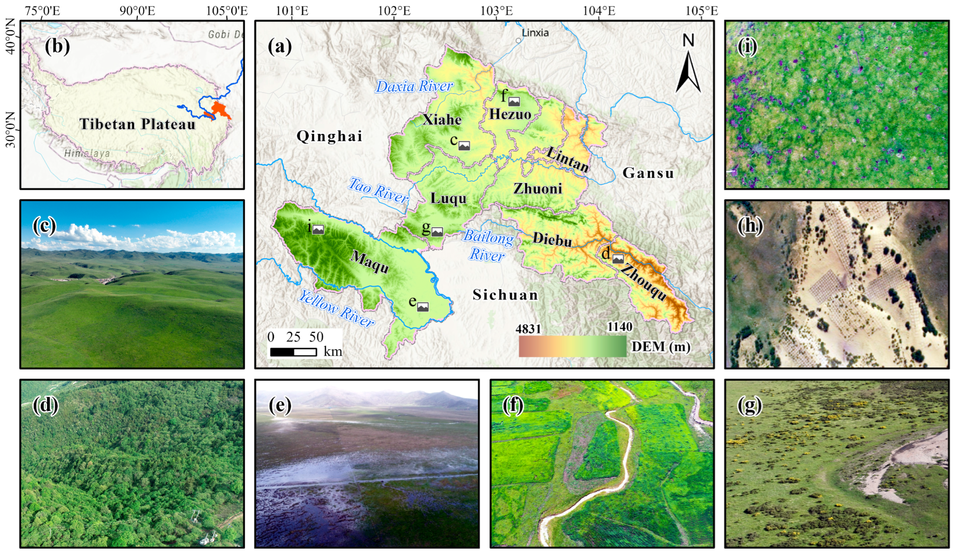
Figure 1. Overview of the study areas. (a,b) Geographic location and elevation of Gannan Prefecture; (cg) photographs of the grassland, forest, wetland, cultivated land, and shrubland, respectively; (h,i) scenes of grassland desertification and rodent damage.
Remotesensing 16 02242 g001
Figure 2. Research framework.
Remotesensing 16 02242 g002
Figure 3. Spatiotemporal distribution of the PGDI from 2000–2020.
Remotesensing 16 02242 g003
Figure 4. Spatiotemporal distribution of the ER levels from 2000–2020.
Remotesensing 16 02242 g004
Figure 5. The ER level transfer matrix. (a) 2000–2005; (b) 2005–2010; (c) 2010–2015; (d) 2015–2020.
Remotesensing 16 02242 g005
Figure 6. The ER level changes from 2000–2020.
Remotesensing 16 02242 g006
Figure 7. Spatiotemporal distribution of the ESI during 2000–2020.
Remotesensing 16 02242 g007
Figure 8. Spatiotemporal distribution of ESs levels during 2000–2020.
Remotesensing 16 02242 g008
Figure 9. The ESs level transfer matrix. (a) 2000–2005, (b) 2005–2010, (c) 2010–2015, (d) 2015–2020.
Remotesensing 16 02242 g009
Figure 10. The ESs level changes from 2000–2020.
Remotesensing 16 02242 g010
Figure 11. Global Moran’s index scatter plot. (a) 2000, (b) 2005, (c) 2010, (d) 2015, (e) 2020, (f) mean.
Remotesensing 16 02242 g011
Figure 12. Local Moran’s index local indicators of spatial correlation clustering plot.
Remotesensing 16 02242 g012
Figure 13. The explanatory power of ecological risk. Note: X1, precipitation; X2, temperature; X3, DEM; X4, slope; X5, aspect; X6, NDVI; X7, evenness index; X8, diversity index; X9, contagion index; X10, land reclamation rate; X11, gross domestic product per capita; X12, fertilizer usage; X13, industrial addition; X14, grazing pressure; X15, urbanization rate.
Remotesensing 16 02242 g013
Figure 14. Results of the interactive detection of the driving factors of ecological risk. Note: X1, precipitation; X2, temperature; X3, DEM; X4, slope; X5, aspect; X6, NDVI; X7, evenness index; X8, diversity index; X9, contagion index; X10, land reclamation rate; X11, gross domestic product per capita; X12, fertilizer usage; X13, industrial addition; X14, grazing pressure; X15, urbanization rate.
Remotesensing 16 02242 g014
Table 1. Data types and descriptions.
DataSpatialData DescriptionsSource
Administrative divisionVector formatThe data were employed for the computation of regional division and result analysisNational Geospatial Information Public Service Cloud Platform
(https://www.tianditu.gov.cn/), accessed on 10 May 2023.
Land use data in 2000–2020Grid cells at 30 m resolutionLand use data were employed for the computation of ESs and landscape ER indexZenodo
(https://doi.org/10.5281/zenodo.5816591), accessed on 10 May 2023.
Digital elevation model dataGrid cells at 1 km resolutionThe data were employed for the computation of ESs index, extract slope data, slope aspect data.Geospatial Data Cloud
(www.gscloud.cn), accessed on 15 June 2023.
Normalized difference vegetation indexGrid cells at 30 m resolutionThe data were used to calculate the driving factors of ERNational Ecological Science Data Center
(https://cstr.cn/15732.11.nesdc.ecodb.rs.2021.012), accessed on 3 May 2023.
Meteorological dataVector and table formatThe data were employed for the computation of each ESsNational Meteorological Information Center
(http://data.cma.cn), accessed on 4 April 2023.
Soil dataGrid cells at 1 km resolutionThe data were employed for the computation of each ESNational Cryosphere Desert Data Center
(http://www.ncdc.ac.cn), accessed on 4 April 2023.
Remoting sensing dataLandsat5 TM/8 OLI image dataThe data were employed for the computation of remoting ecological index and fractional vegetation coverageGoogle Earth Engine
(https://earthengine.google.com/), accessed on 8 May 2023.
Above-grassland biomass (AGB)Grid cells at 250 m resolutionThe data were employed for the computation of the grass–livestock balance indexTPDC
(https://doi.org/10.11888/Terre.tpdc.272587), accessed on 13 April 2023.
Population densityGrid cells at 100 m resolutionThe data were employed for the computation of the grass–livestock balance indexWorldPop
(https://hub.worldpop.org/geodata/listing?id=16), accessed on 4 April 2023.
Statistical dataTable or text formatThe data were used to obtain the fertilizer usage, urbanization rate, gross domestic product, and so onGannan Prefecture Bureau of Statistics Site
(http://www.gnzrmzf.gov.cn/zfxxgk/fdzdgknr1/tjxx/tjnj2.htm), accessed on 15 June 2023.
Geographical dataVector
format
The data were employed to extract residential and road dataOpenStreetMap
(http://download.geofabrik.de/), accessed on 19 April 2023.
Disclaimer/Publisher’s Note: The statements, opinions and data contained in all publications are solely those of the individual author(s) and contributor(s) and not of MDPI and/or the editor(s). MDPI and/or the editor(s) disclaim responsibility for any injury to people or property resulting from any ideas, methods, instructions or products referred to in the content.