


Towards Urban Digital Twins: A Workflow for Procedural Visualization Using Geospatial Data

 , , , and
Abstract
1. Introduction
- First, to develop a methodology for integrating various data sources for urban modeling.
- Second, to establish a reproducible and procedural workflow for generating urban digital twins.
- Finally, to incorporate effective visualization techniques to enhance the interactivity and scalability of the digital twins.
2. Related Work
2.1. Methods for Efficient Workflows in 3D Building Reconstruction
2.2. Large-Scale Data Visualization in the Production of DTs
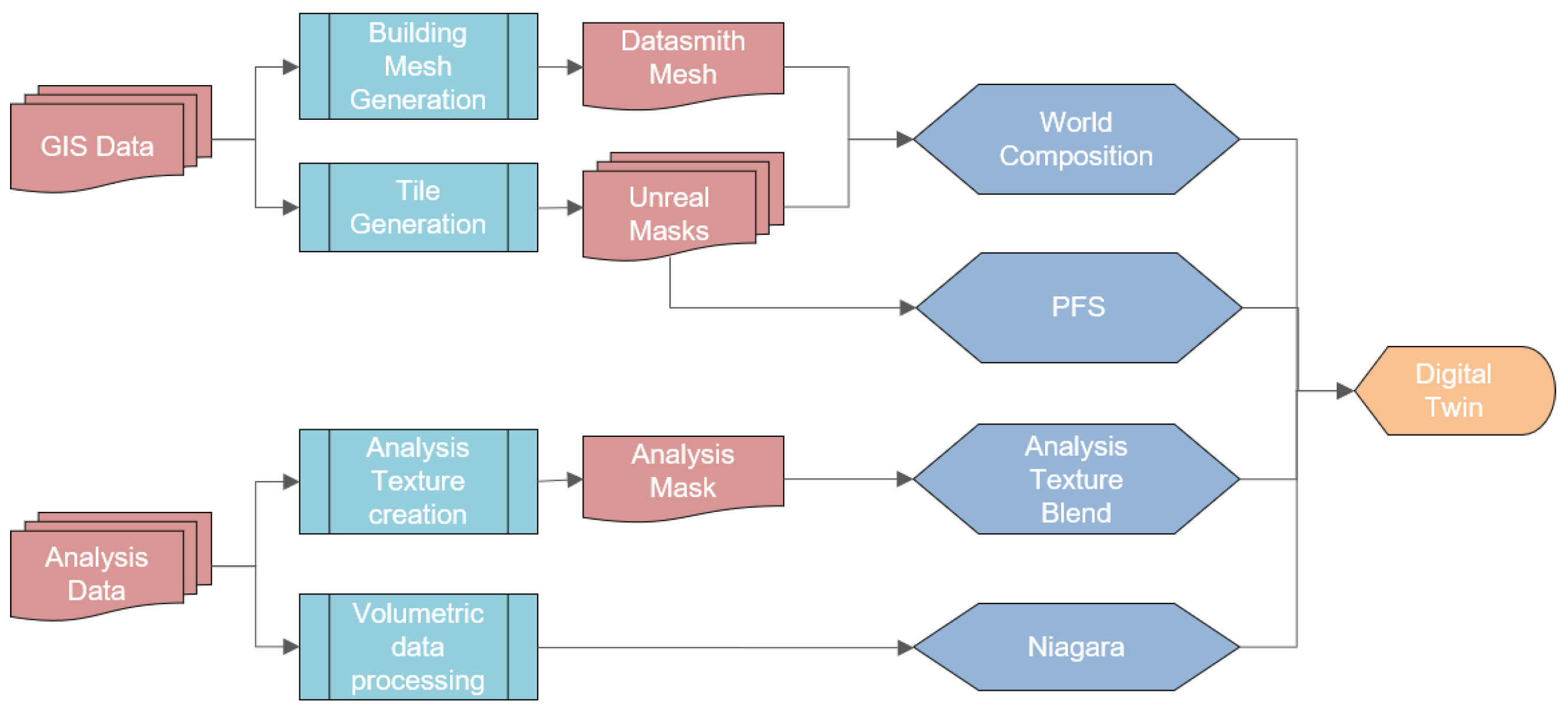
3. Materials and Methods
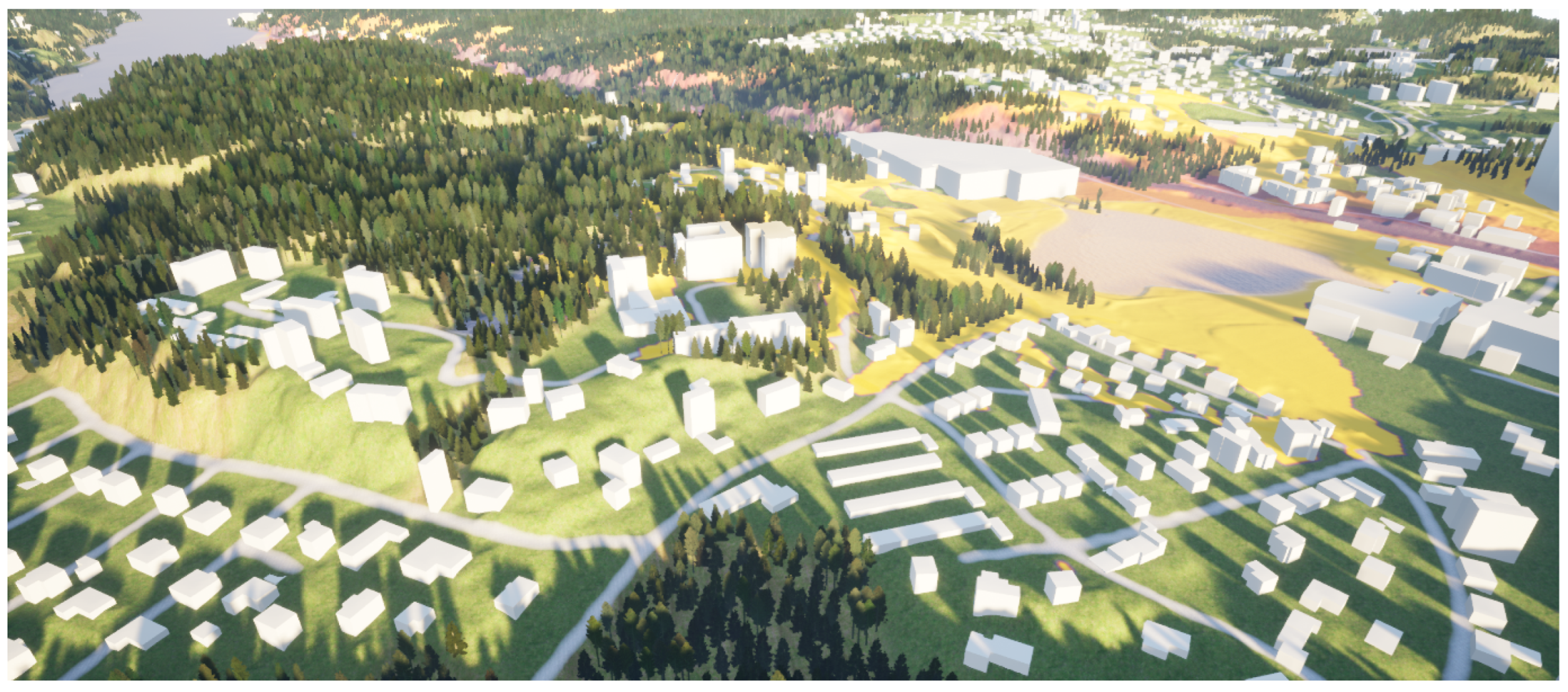
3.1. World Creation
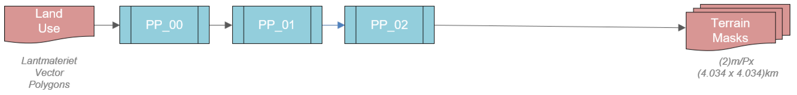
3.1.1. Terrain
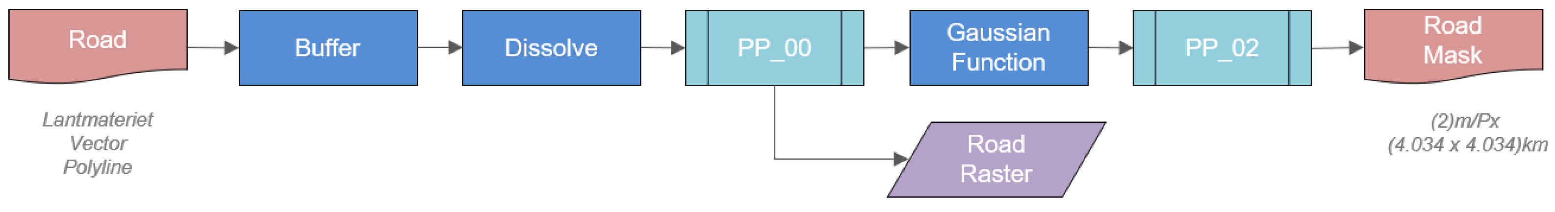
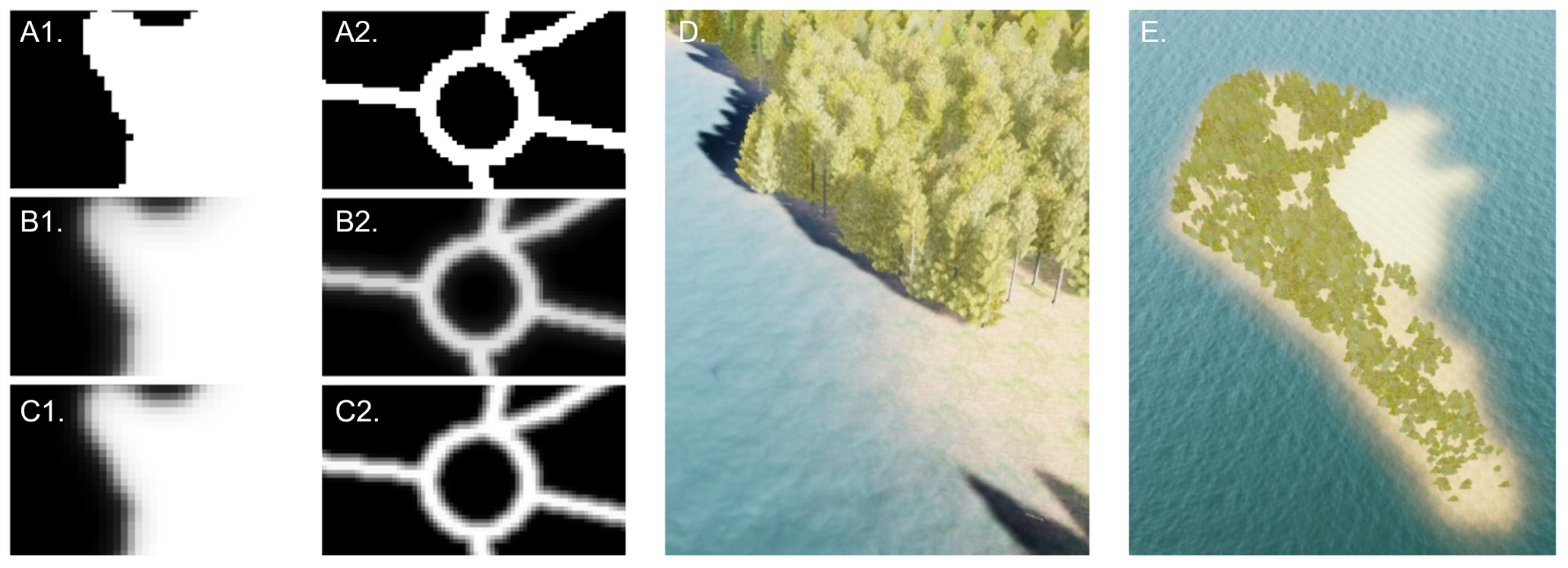
3.1.2. Roads
3.1.3. Vegetation
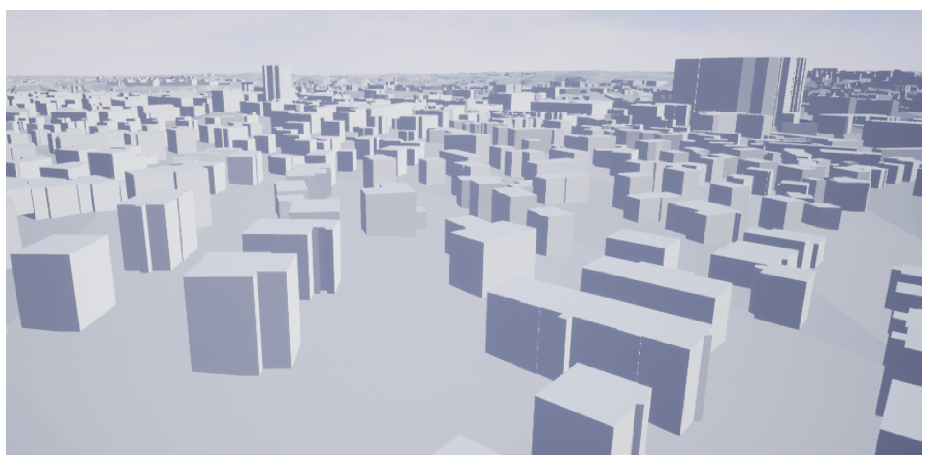
3.1.4. Buildings
3.2. Unreal Engine Workflow
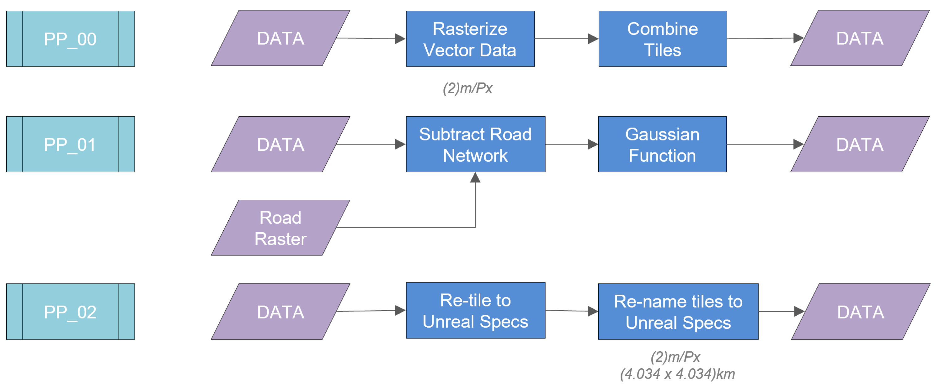
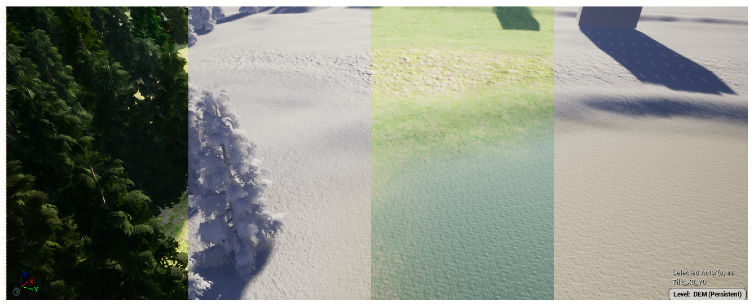
3.2.1. Integration of Landscape Tiles
3.2.2. Procedural Landscape Material
3.3. Data Visualization
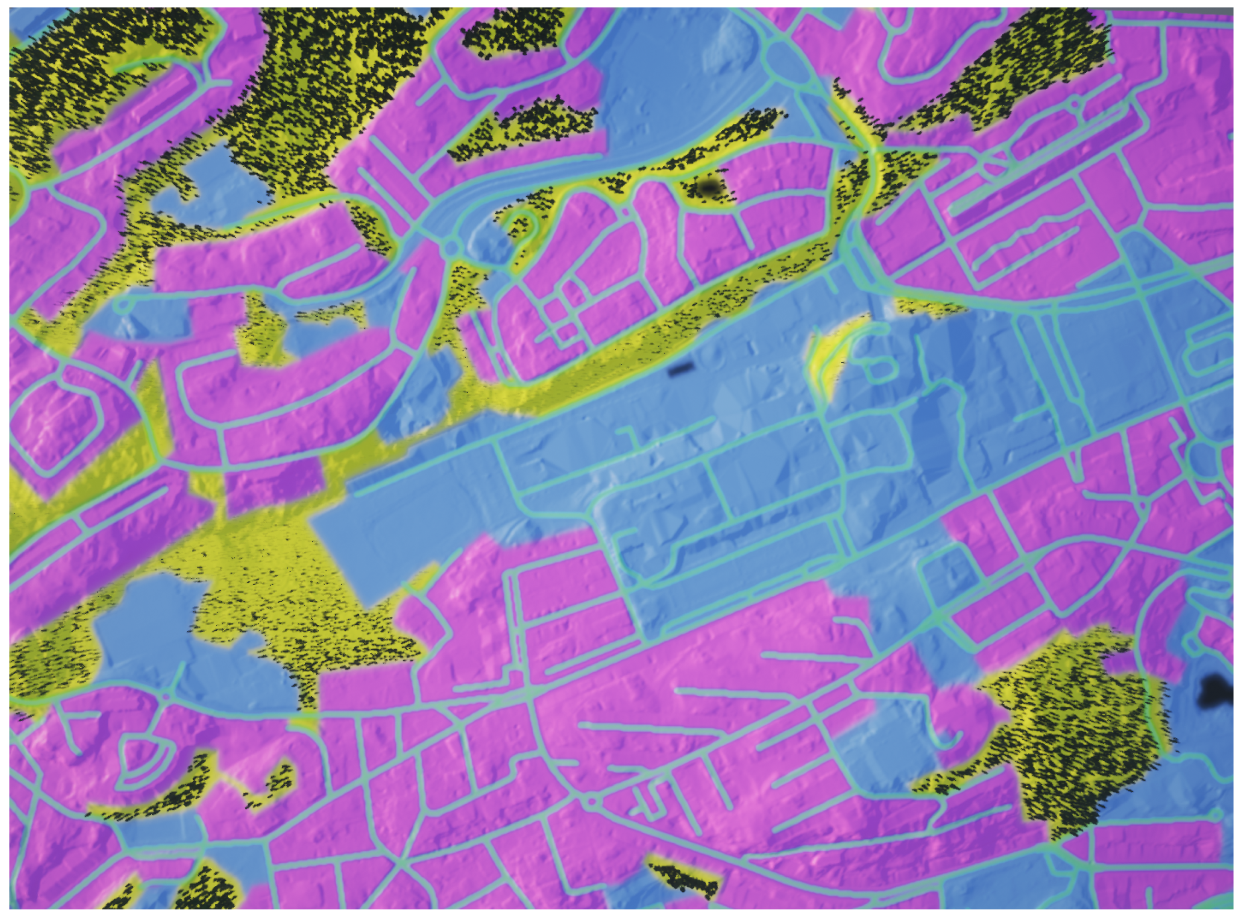
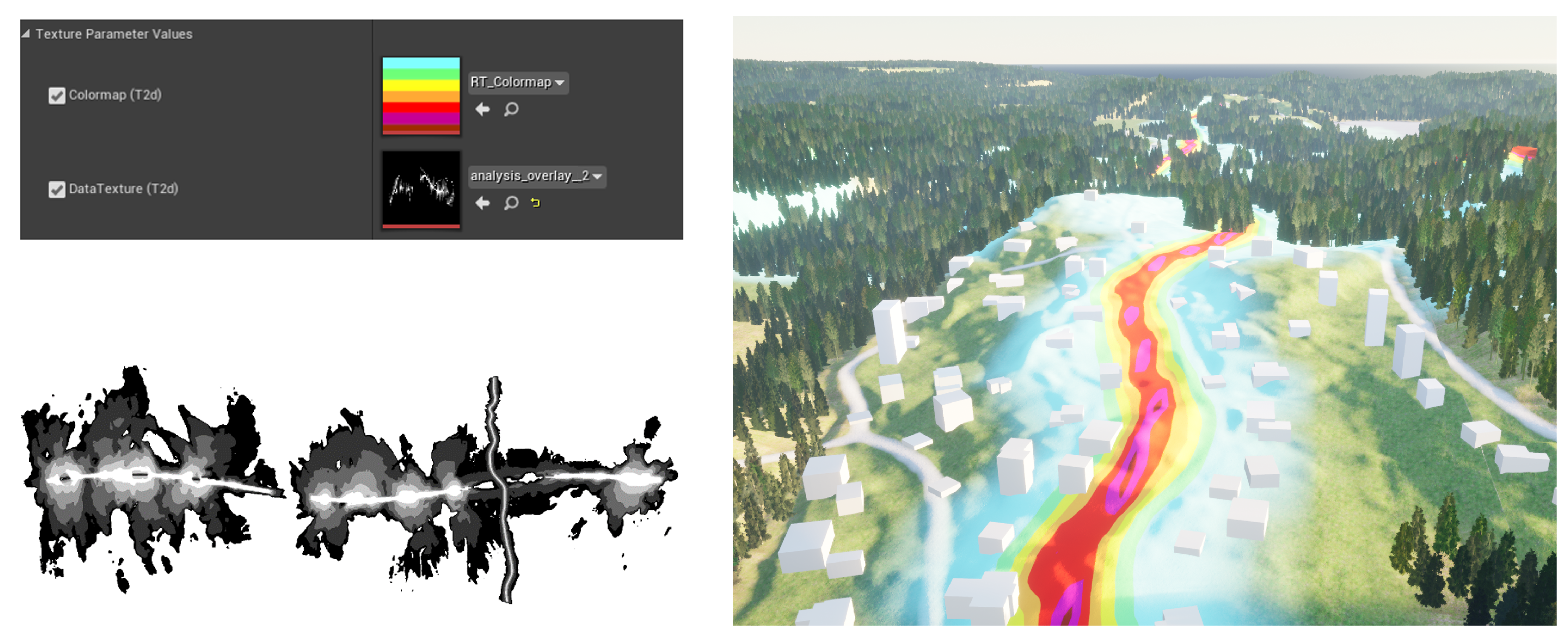
3.3.1. Isoline Data
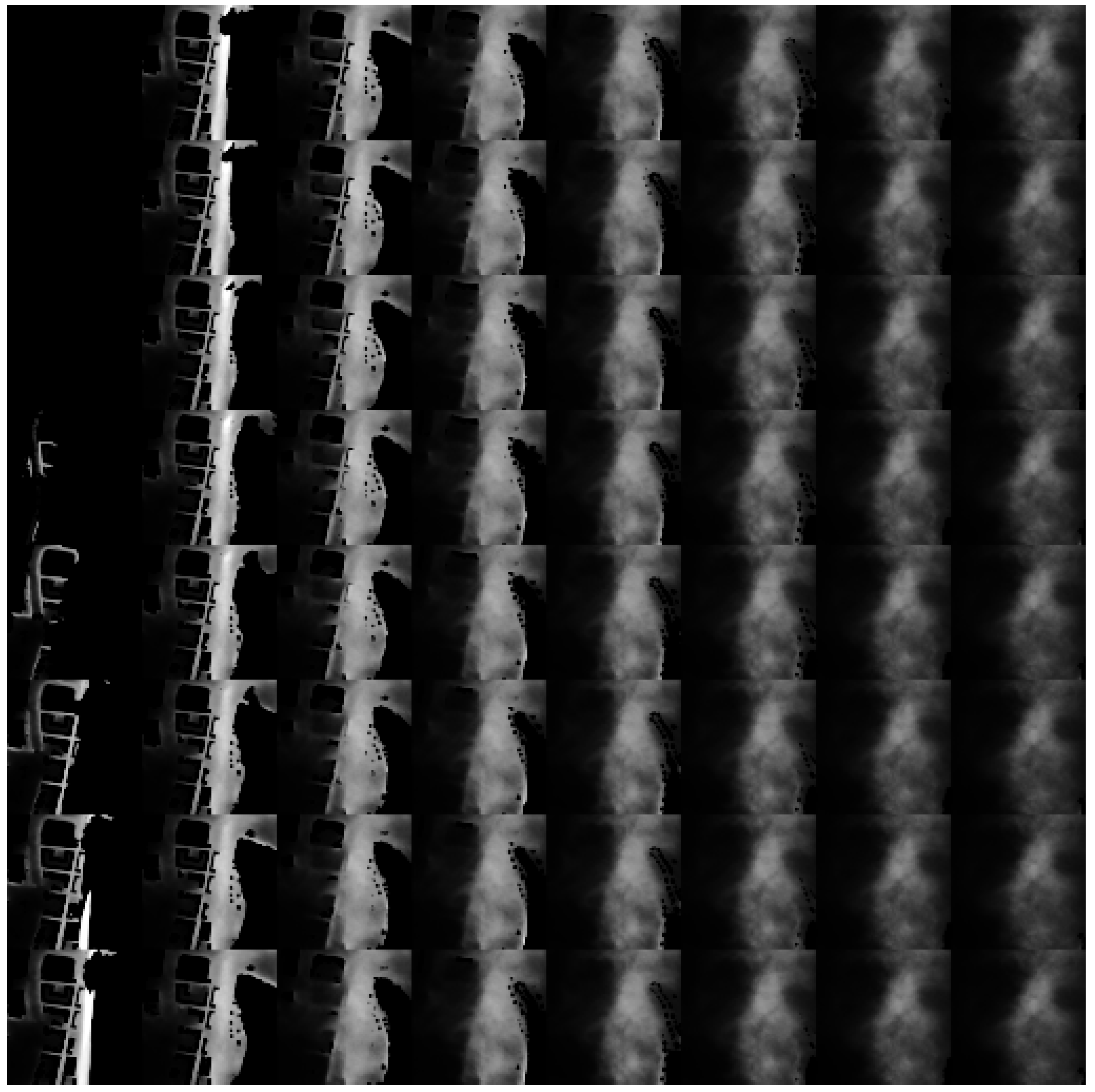
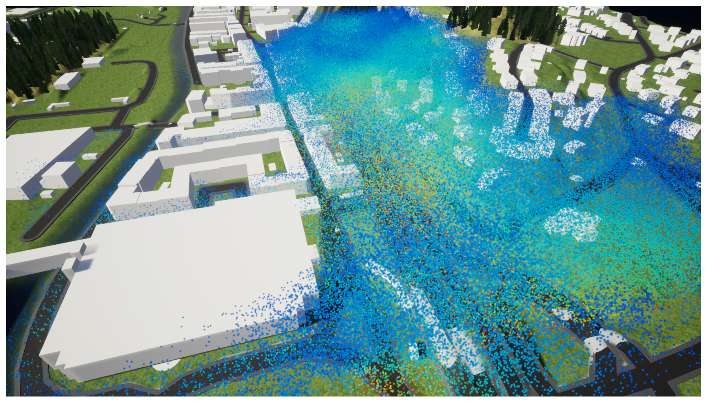
3.3.2. Volumetric Data
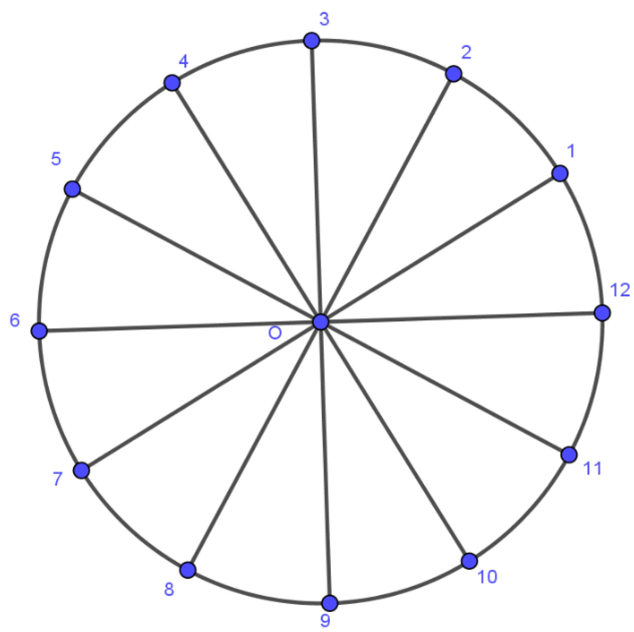
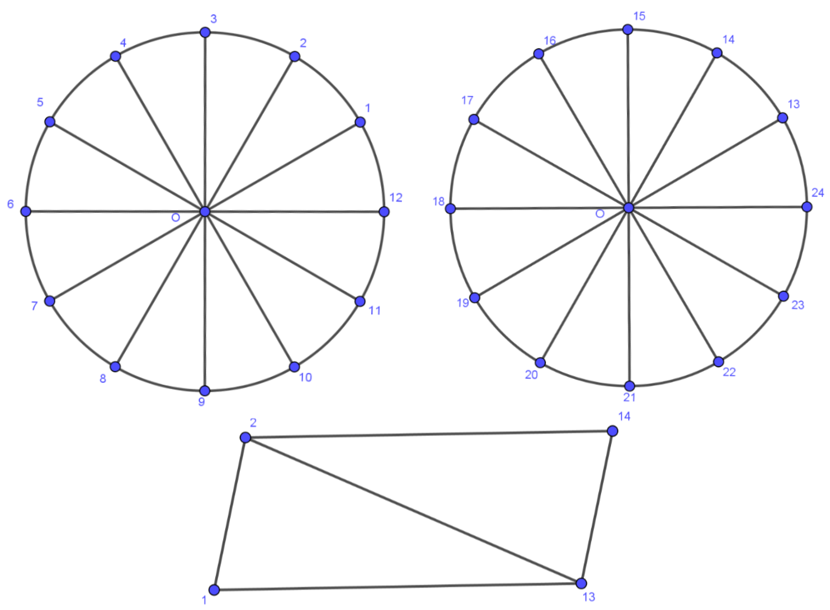
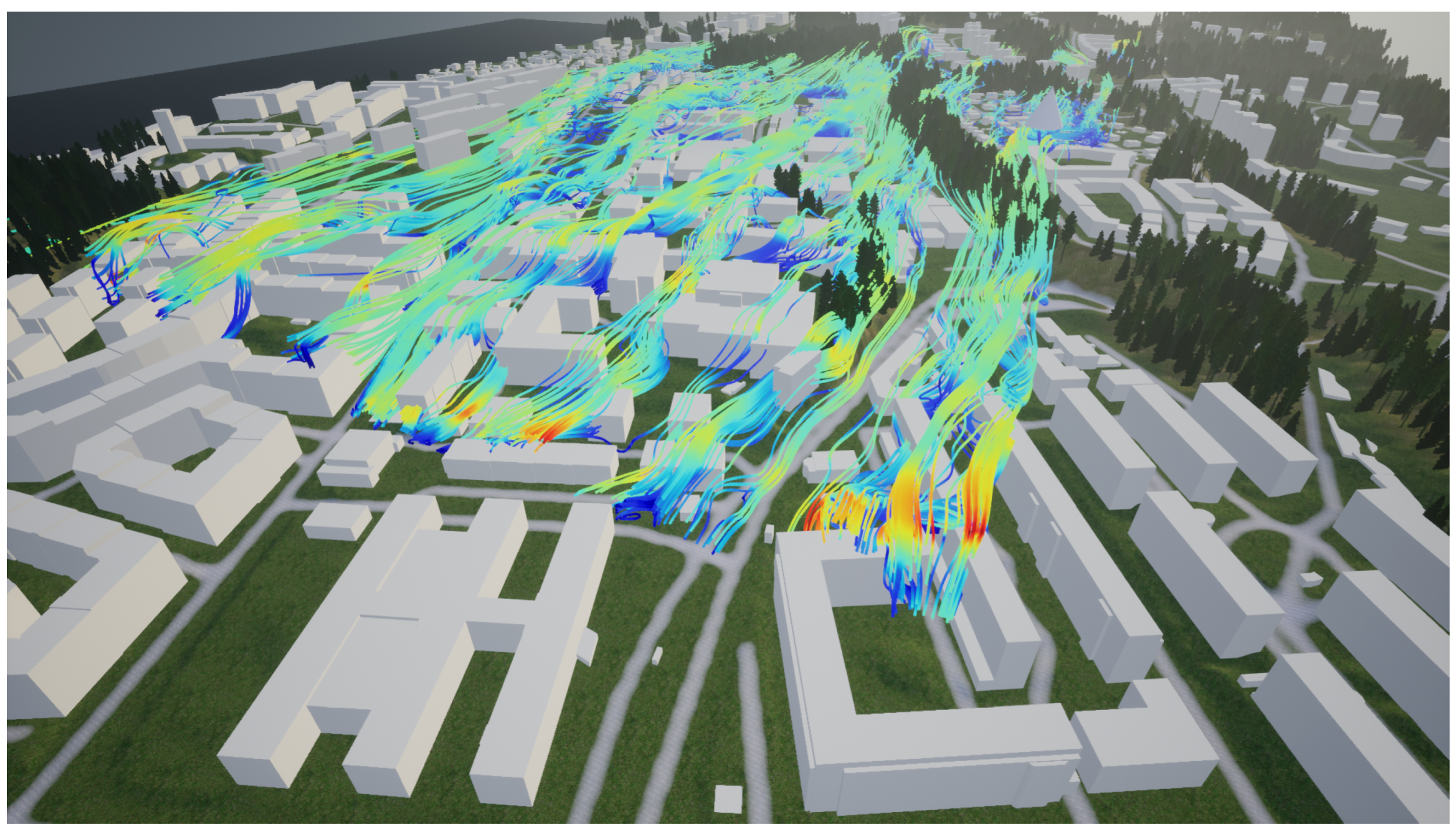
3.3.3. Particle Streamlines
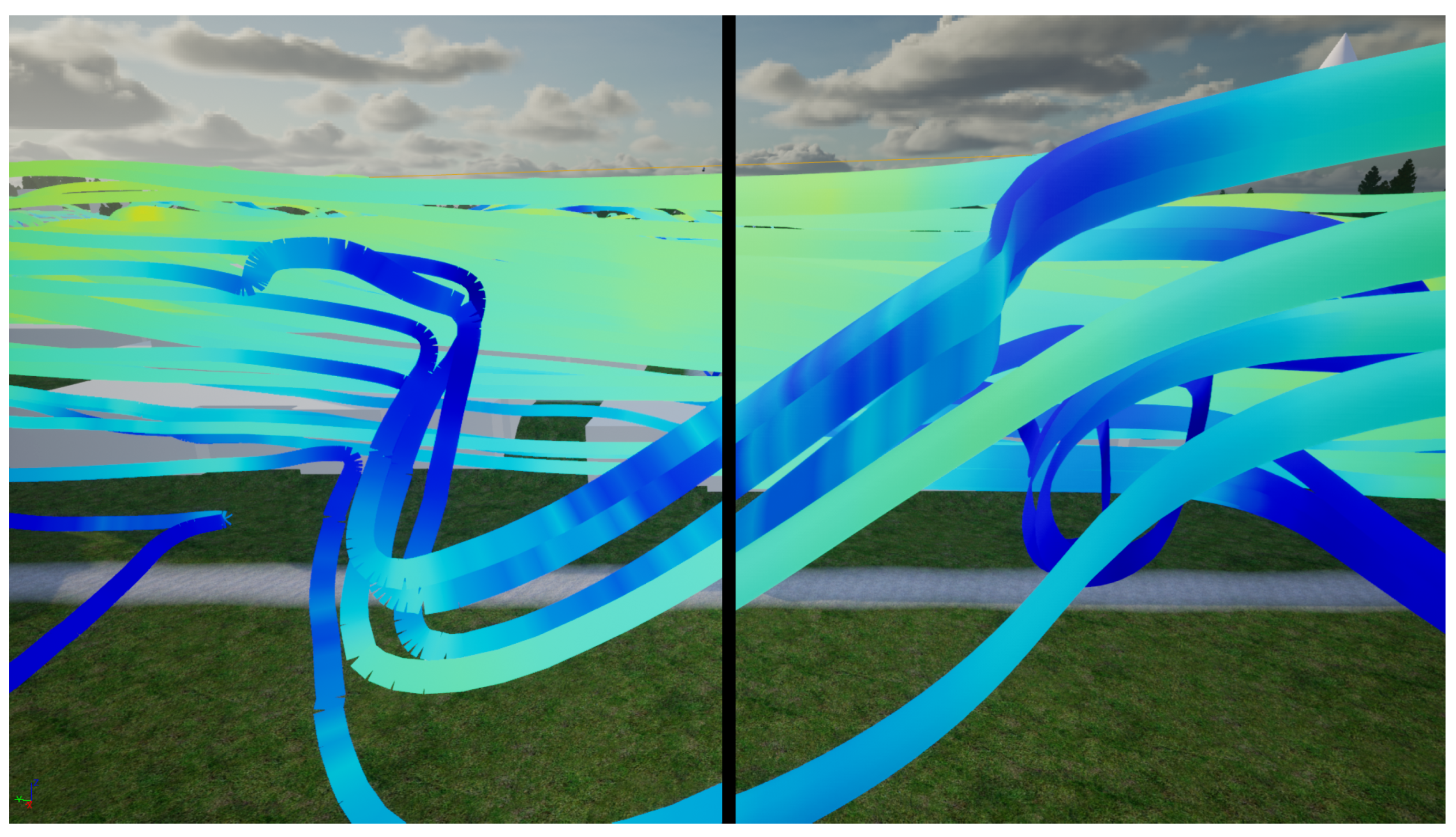
Procedural Meshed Streamlines
- Generating vertices around each parsed point of the streamline;
- Creating triangles between the generated vertices;
- Connecting sequential vertices that belong to different points.
4. Results
4.1. World Creation
4.1.1. Generating Assets
4.1.2. Unreal Engine Workflow
4.2. Data Visualization
4.2.1. Isoline Data
4.2.2. Volumetric Data
4.2.3. Streamlines
5. Limitations and Discussion
6. Conclusions
7. Declaration of AI in the Writing Process
Author Contributions
Funding
Data Availability Statement
Acknowledgments
Conflicts of Interest
References
- Ketzler, B.; Naserentin, V.; Latino, F.; Zangelidis, C.; Thuvander, L.; Logg, A. Digital Twins for Cities: A State of the Art Review. Built Environ. 2020, 46, 547–573. [Google Scholar] [CrossRef]
- Gil, J. City Information Modelling: A Conceptual Framework for Research and Practice in Digital Urban Planning. Built Environ. 2020, 46, 501–527. [Google Scholar] [CrossRef]
- Logg, A.; Mardal, K.A.; Wells, G. Automated Solution of Differential Equations by the Finite Element Method: The FEniCS Book; Springer Science & Business Media: Berlin/Heidelberg, Germany, 2012; Volume 84. [Google Scholar]
- Girindran, R.; Boyd, D.S.; Rosser, J.; Vijayan, D.; Long, G.; Robinson, D. On the Reliable Generation of 3D City Models from Open Data. Urban Sci. 2020, 4, 47. [Google Scholar] [CrossRef]
- Pađen, I.; García-Sánchez, C.; Ledoux, H. Towards automatic reconstruction of 3D city models tailored for urban flow simulations. Front. Built Environ. 2022, 8, 899332. [Google Scholar] [CrossRef]
- Ledoux, H.; Biljecki, F.; Dukai, B.; Kumar, K.; Peters, R.; Stoter, J.; Commandeur, T. 3dfier: Automatic reconstruction of 3D city models. J. Open Source Softw. 2021, 6, 2866. [Google Scholar] [CrossRef]
- Batty, M. Digital twins. Environ. Plan. Urban Anal. City Sci. 2018, 45, 817–820. [Google Scholar] [CrossRef]
- Ham, Y.; Kim, J. Participatory sensing and digital twin city: Updating virtual city models for enhanced risk-informed decision-making. J. Manag. Eng. 2020, 36, 04020005. [Google Scholar] [CrossRef]
- Latino, F.; Naserentin, V.; Öhrn, E.; Shengdong, Z.; Fjeld, M.; Thuvander, L.; Logg, A. Virtual City@ Chalmers: Creating a prototype for a collaborative early stage urban planning AR application. Proc. eCAADe RIS 2019, 137–147. Available online: https://www.researchgate.net/profile/Fabio-Latino/publication/333134046_Virtual_CityChalmers_Creating_a_prototype_for_a_collaborative_early_stage_urban_planning_AR_application/links/5cdd4e62299bf14d959d0cb7/Virtual-CityChalmers-Creating-a-prototype-for-a-collaborative-early-stage-urban-planning-AR-application.pdf (accessed on 19 March 2024).
- Muñumer Herrero, E.; Ellul, C.; Cavazzi, S. Exploring Existing 3D Reconstruction Tools for the Generation of 3D City Models at Various Lod from a Single Data Source. ISPRS Ann. Photogramm. Remote Sens. Spat. Inf. Sci. 2022, X-4/W2, 209–216. [Google Scholar] [CrossRef]
- Nan, L.; Wonka, P. PolyFit: Polygonal Surface Reconstruction From Point Clouds. In Proceedings of the IEEE International Conference on Computer Vision, Venice, Italy, 22–29 October 2017; pp. 2353–2361. [Google Scholar]
- Poux, F. 5-Step Guide to Generate 3D Meshes from Point Clouds with Python. 2021. Available online: https://towardsdatascience.com/5-step-guide-to-generate-3d-meshes-from-point-clouds-with-python-36bad397d8ba (accessed on 3 May 2023).
- Schnabel, R.; Wahl, R.; Klein, R. Efficient RANSAC for Point-Cloud Shape Detection. Comput. Graph. Forum 2007, 26, 214–226. [Google Scholar] [CrossRef]
- Wang, H. Design of Commercial Building Complex Based on 3D Landscape Interaction. Sci. Program. 2022, 2022, 7664803. [Google Scholar] [CrossRef]
- Coors, V.; Betz, M.; Duminil, E. A Concept of Quality Management of 3D City Models Supporting Application-Specific Requirements. PFG J. Photogramm. Remote Sens. Geoinf. Sci. 2020, 88, 3–14. [Google Scholar] [CrossRef]
- García-Sánchez, C.; Vitalis, S.; Paden, I.; Stoter, J. The impact of level of detail in 3D city models for cfd-based wind flow simulations. Int. Arch. Photogramm. Remote Sens. Spat. Inf. Sci. 2021, XLVI-4/W4-2021, 67–72. [Google Scholar] [CrossRef]
- Deininger, M.E.; von der Grün, M.; Piepereit, R.; Schneider, S.; Santhanavanich, T.; Coors, V.; Voß, U. A Continuous, Semi-Automated Workflow: From 3D City Models with Geometric Optimization and CFD Simulations to Visualization of Wind in an Urban Environment. ISPRS Int. J. Geo-Inf. 2020, 9, 657. [Google Scholar] [CrossRef]
- Kolbe, T.H.; Donaubauer, A. Semantic 3D City Modeling and BIM. In Urban Informatics; Shi, W., Goodchild, M.F., Batty, M., Kwan, M.P., Zhang, A., Eds.; The Urban Book Series; Springer: Singapore, 2021; pp. 609–636. [Google Scholar] [CrossRef]
- Dimitrov, H.; Petrova-Antonova, D. 3D city model as a first step towards digital twin of Sofia city. Int. Arch. Photogramm. Remote Sens. Spat. Inf. Sci. 2021, 43, 23–30. [Google Scholar] [CrossRef]
- Singla, J.G.; Padia, K. A Novel Approach for Generation and Visualization of Virtual 3D City Model Using Open Source Libraries. J. Indian Soc. Remote Sens. 2021, 49, 1239–1244. [Google Scholar] [CrossRef]
- OpenStreetMap Contributors. OpenStreetMap. 2024. Available online: https://www.openstreetmap.org (accessed on 22 May 2024).
- Pepe, M.; Costantino, D.; Alfio, V.S.; Vozza, G.; Cartellino, E. A Novel Method Based on Deep Learning, GIS and Geomatics Software for Building a 3D City Model from VHR Satellite Stereo Imagery. ISPRS Int. J. Geo-Inf. 2021, 10, 697. [Google Scholar] [CrossRef]
- Buyukdemircioglu, M.; Kocaman, S. Reconstruction and Efficient Visualization of Heterogeneous 3D City Models. Remote Sens. 2020, 12, 2128. [Google Scholar] [CrossRef]
- Döllner, J.; Buchholz, H. Continuous Level-of-Detail Modeling of Buildings in 3D City Models. In Proceedings of the 13th Annual ACM International Workshop on Geographic Information Systems, GIS ’05, Bremen, Germany, 4–5 November 2005; pp. 173–181. [Google Scholar] [CrossRef]
- Ortega, S.; Santana, J.M.; Wendel, J.; Trujillo, A.; Murshed, S.M. Generating 3D City Models from Open LiDAR Point Clouds: Advancing Towards Smart City Applications. In Open Source Geospatial Science for Urban Studies: The Value of Open Geospatial Data; Mobasheri, A., Ed.; Lecture Notes in Intelligent Transportation and Infrastructure; Springer International Publishing: Cham, Switzerland, 2021; pp. 97–116. [Google Scholar] [CrossRef]
- Katal, A.; Mortezazadeh, M.; Wang, L.L.; Yu, H. Urban Building Energy and Microclimate Modeling–From 3D City Generation to Dynamic Simulations. Energy 2022, 251, 123817. [Google Scholar] [CrossRef]
- Peters, R.; Dukai, B.; Vitalis, S.; van Liempt, J.; Stoter, J. Automated 3D reconstruction of LoD2 and LoD1 models for all 10 million buildings of the Netherlands. Photogramm. Eng. Remote Sens. 2022, 88, 165–170. [Google Scholar] [CrossRef]
- Alomía, G.; Loaiza, D.; Zúñiga, C.; Luo, X.; Asoreycacheda, R. Procedural modeling applied to the 3D city model of bogota: A case study. Virtual Real. Intell. Hardw. 2021, 3, 423–433. [Google Scholar] [CrossRef]
- Chen, Z.; Ledoux, H.; Khademi, S.; Nan, L. Reconstructing Compact Building Models from Point Clouds Using Deep Implicit Fields. ISPRS J. Photogramm. Remote Sens. 2022, 194, 58–73. [Google Scholar] [CrossRef]
- Diakite, A.; Ng, L.; Barton, J.; Rigby, M.; Williams, K.; Barr, S.; Zlatanova, S. Liveable City Digital Twin: A Pilot Project for the City of Liverpool (nsw, Australia). ISPRS Ann. Photogramm. Remote Sens. Spat. Inf. Sci. 2022, 10, 45–52. [Google Scholar] [CrossRef]
- Biljecki, F.; Stoter, J.; Ledoux, H.; Zlatanova, S.; Çöltekin, A. Applications of 3D city models: State of the art review. ISPRS Int. J. Geo-Inf. 2015, 4, 2842–2889. [Google Scholar] [CrossRef]
- Fuller, A.; Fan, Z.; Day, C.; Barlow, C. Digital twin: Enabling technologies, challenges and open research. IEEE Access 2020, 8, 108952–108971. [Google Scholar] [CrossRef]
- Lei, B.; Janssen, P.; Stoter, J.; Biljecki, F. Challenges of urban digital twins: A systematic review and a Delphi expert survey. Autom. Constr. 2023, 147, 104716. [Google Scholar] [CrossRef]
- Yu, J.; Stettler, M.E.; Angeloudis, P.; Hu, S.; Chen, X.M. Urban network-wide traffic speed estimation with massive ride-sourcing GPS traces. Transp. Res. Part Emerg. Technol. 2020, 112, 136–152. [Google Scholar] [CrossRef]
- Chen, B.; Xu, B.; Gong, P. Mapping essential urban land use categories (EULUC) using geospatial big data: Progress, challenges, and opportunities. Big Earth Data 2021, 5, 410–441. [Google Scholar] [CrossRef]
- Ferré-Bigorra, J.; Casals, M.; Gangolells, M. The adoption of urban digital twins. Cities 2022, 131, 103905. [Google Scholar] [CrossRef]
- Dembski, F.; Wössner, U.; Letzgus, M.; Ruddat, M.; Yamu, C. Urban digital twins for smart cities and citizens: The case study of Herrenberg, Germany. Sustainability 2020, 12, 2307. [Google Scholar] [CrossRef]
- Shahat, E.; Hyun, C.T.; Yeom, C. City digital twin potentials: A review and research agenda. Sustainability 2021, 13, 3386. [Google Scholar] [CrossRef]
- Mylonas, G.; Kalogeras, A.; Kalogeras, G.; Anagnostopoulos, C.; Alexakos, C.; Muñoz, L. Digital twins from smart manufacturing to smart cities: A survey. IEEE Access 2021, 9, 143222–143249. [Google Scholar] [CrossRef]
- Jeddoub, I.; Nys, G.A.; Hajji, R.; Billen, R. Digital Twins for cities: Analyzing the gap between concepts and current implementations with a specific focus on data integration. Int. J. Appl. Earth Obs. Geoinf. 2023, 122, 103440. [Google Scholar] [CrossRef]
- Zhao, Y.; Wang, Y.; Zhang, J.; Fu, C.W.; Xu, M.; Moritz, D. KD-Box: Line-segment-based KD-tree for Interactive Exploration of Large-scale Time-Series Data. IEEE Trans. Vis. Comput. Graph. 2022, 28, 890–900. [Google Scholar] [CrossRef] [PubMed]
- Jaillot, V.; Servigne, S.; Gesquière, G. Delivering time-evolving 3D city models for web visualization. Int. J. Geogr. Inf. Sci. 2020, 34, 2030–2052. [Google Scholar] [CrossRef]
- Wu, Z.; Wang, N.; Shao, J.; Deng, G. GPU ray casting method for visualizing 3D pipelines in a virtual globe. Int. J. Digit. Earth 2019, 12, 428–441. [Google Scholar] [CrossRef]
- Kon, F.; Ferreira, É.C.; de Souza, H.A.; Duarte, F.; Santi, P.; Ratti, C. Abstracting mobility flows from bike-sharing systems. Public Transp. 2021, 14, 545–581. [Google Scholar] [CrossRef] [PubMed]
- Xu, M.; Liu, H.; Yang, H. A deep learning based multi-block hybrid model for bike-sharing supply-demand prediction. IEEE Access 2020, 8, 85826–85838. [Google Scholar] [CrossRef]
- Jiang, Z.; Liu, Y.; Fan, X.; Wang, C.; Li, J.; Chen, L. Understanding urban structures and crowd dynamics leveraging large-scale vehicle mobility data. Front. Comput. Sci. 2020, 14, 145310. [Google Scholar] [CrossRef]
- Lu, Q.; Xu, W.; Zhang, H.; Tang, Q.; Li, J.; Fang, R. ElectricVIS: Visual analysis system for power supply data of smart city. J. Supercomput. 2020, 76, 793–813. [Google Scholar] [CrossRef]
- Deng, Z.; Weng, D.; Liang, Y.; Bao, J.; Zheng, Y.; Schreck, T.; Xu, M.; Wu, Y. Visual cascade analytics of large-scale spatiotemporal data. IEEE Trans. Vis. Comput. Graph. 2021, 28, 2486–2499. [Google Scholar] [CrossRef]
- Gardony, A.L.; Martis, S.B.; Taylor, H.A.; Brunye, T.T. Interaction strategies for effective augmented reality geo-visualization: Insights from spatial cognition. Hum. Comput. Interact. 2021, 36, 107–149. [Google Scholar] [CrossRef]
- Xu, H.; Berres, A.; Tennille, S.A.; Ravulaparthy, S.K.; Wang, C.; Sanyal, J. Continuous Emulation and Multiscale Visualization of Traffic Flow Using Stationary Roadside Sensor Data. IEEE Trans. Intell. Transp. Syst. 2021, 23, 10530–10541. [Google Scholar] [CrossRef]
- Lee, A.; Chang, Y.S.; Jang, I. Planetary-Scale Geospatial Open Platform Based on the Unity3D Environment. Sensors 2020, 20, 5967. [Google Scholar] [CrossRef]
- Li, Q.; Liu, Y.; Chen, L.; Yang, X.; Peng, Y.; Yuan, X.; Lalith, M. SEEVis: A Smart Emergency Evacuation Plan Visualization System with Data-Driven Shot Designs. Comput. Graph. Forum 2020, 39, 523–535. [Google Scholar] [CrossRef]
- Lantmäteriet, the Swedish Mapping, Cadastral and Land Registration Authority. 2022. Available online: https://lantmateriet.se/ (accessed on 3 May 2023).
- Logg, A.; Naserentin, V.; Wästberg, D. DTCC Builder: A mesh generator for automatic, efficient, and robust mesh generation for large-scale city modeling and simulation. J. Open Source Softw. 2023, 8, 4928. [Google Scholar] [CrossRef]
- Mark, A.; Rundqvist, R.; Edelvik, F. Comparison between different immersed boundary conditions for simulation of complex fluid flows. Fluid Dyn. Mater. Process. 2011, 7, 241–258. [Google Scholar]
- Wind Nuisance and Wind Hazard in the Built Environment. 2006. Available online: https://connect.nen.nl/Standard/Detail/107592 (accessed on 22 May 2024).
- Thuvander, L.; Somanath, S.; Hollberg, A. Procedural Digital Twin Generation for Co-Creating in VR Focusing on Vegetation. Int. Arch. Photogramm. Remote Sens. Spat. Inf. Sci. 2022, 48, 189–196. [Google Scholar] [CrossRef]
- Kolibarov, N.; Wästberg, D.; Naserentin, V.; Petrova-Antonova, D.; Ilieva, S.; Logg, A. Roof Segmentation Towards Digital Twin Generation in LoD2+ Using Deep Learning. IFAC-PapersOnLine 2022, 55, 173–178. [Google Scholar] [CrossRef]
- Naserentin, V.; Spaias, G.; Kaimakamidis, A.; Somanath, S.; Logg, A.; Mitkov, R.; Pantusheva, M.; Dimara, A.; Krinidis, S.; Anagnostopoulos, C.N.; et al. Data Collection & Wrangling Towards Machine Learning in LoD2+ Urban Models Generation. In Proceedings of the Artificial Intelligence Applications and Innovations: 20th International Conference, AIAI 2024, Corfu, Greece, 27–30 June 2024. [Google Scholar]
- Nordmark, N.; Ayenew, M. Window detection in facade imagery: A deep learning approach using mask R-CNN. arXiv 2021, arXiv:2107.10006. [Google Scholar]
- Harrison, J.; Hollberg, A.; Yu, Y. Scalability in Building Component Data Annotation: Enhancing Facade Material Classification with Synthetic Data. arXiv 2024, arXiv:2404.08557. [Google Scholar]
- Gonzalez-Caceres, A.; Hunger, F.; Forssén, J.; Somanath, S.; Mark, A.; Naserentin, V.; Bohlin, J.; Logg, A.; Wästberg, B.; Komisarczyk, D.; et al. Towards digital twinning for multi-domain simulation workflows in urban design: A case study in Gothenburg. J. Build. Perform. Simul. 2024, 1–22. [Google Scholar] [CrossRef]
- Forssen, J.; Hostmad, P.; Wastberg, B.S.; Billger, M.; Ogren, M.; Latino, F.; Naserentin, V.; Eleftheriou, O. An urban planning tool demonstrator with auralisation and visualisation of the sound environment. In Proceedings of the Forum Acusticum, Lyon, France, 7–11 December 2020; pp. 869–871. [Google Scholar]
- Wang, X.; Teigland, R.; Hollberg, A. Identifying influential architectural design variables for early-stage building sustainability optimization. Build. Environ. 2024, 252, 111295. [Google Scholar] [CrossRef]
- Sepasgozar, S.M. Differentiating digital twin from digital shadow: Elucidating a paradigm shift to expedite a smart, sustainable built environment. Buildings 2021, 11, 151. [Google Scholar] [CrossRef]
- Qian, C.; Liu, X.; Ripley, C.; Qian, M.; Liang, F.; Yu, W. Digital twin—Cyber replica of physical things: Architecture, applications and future research directions. Future Internet 2022, 14, 64. [Google Scholar] [CrossRef]
- Stahre Wästberg, B.; Billger, M.; Adelfio, M. A user-based look at visualization tools for environmental data and suggestions for improvement—An inventory among city planners in Gothenburg. Sustainability 2020, 12, 2882. [Google Scholar] [CrossRef]
- Logg, A.; Naserentin, V. Digital Twin Cities Platform—Builder. 2021. Available online: https://github.com/dtcc-platform/dtcc-builder (accessed on 3 May 2023).
- Shewchuk, J.R. Triangle: Engineering a 2D Quality Mesh Generator and Delaunay Triangulator. In Proceedings of the Workshop on Applied Computational Geometry, Philadelphia, PA, USA, 27–28 May 1996; Springer: Berlin/Heidelberg, Germany, 1996; pp. 203–222. [Google Scholar]
- GEOS Contributors. GEOS Coordinate Transformation Software Library; Open Source Geospatial Foundation: Chicago, IL, USA, 2021. [Google Scholar]
- GDAL/OGR Contributors. GDAL/OGR Geospatial Data Abstraction Software Library; Open Source Geospatial Foundation: Chicago, IL, USA, 2020. [Google Scholar]


| Swedish Name | English Name | Description | Format |
|---|---|---|---|
| Bebyggelse | Property map | Building footprints as closed polygons | ShapeFile (*.shp) |
| Kommunikation | Transport networks | Transportation network as center lines | ShapeFile (*.shp) |
| Markdata | Land data | Land-use classification as closed polygons | ShapeFile (*.shp) |
| Höjddata | Elevation data | Ground elevation data as raster images | Tagged Image Format (*.TIF) |
| Laserdata | Laser data | LiDAR scan data as point clouds | Zipped LiDAR Aerial Survey (*.LAZ) |
| Streamlines Number | Procedural Streamlines | Particle Streamlines |
|---|---|---|
| 1003 | 12 ms | 5 ms |
| 4158 | 47 ms | 12 ms |
| 8316 | 134 ms | 51 ms |
| 12,474 | 247 ms | 127 ms |
Disclaimer/Publisher’s Note: The statements, opinions and data contained in all publications are solely those of the individual author(s) and contributor(s) and not of MDPI and/or the editor(s). MDPI and/or the editor(s) disclaim responsibility for any injury to people or property resulting from any ideas, methods, instructions or products referred to in the content. |
© 2024 by the authors. Licensee MDPI, Basel, Switzerland. This article is an open access article distributed under the terms and conditions of the Creative Commons Attribution (CC BY) license (https://creativecommons.org/licenses/by/4.0/).
Share and Cite
Somanath, S.; Naserentin, V.; Eleftheriou, O.; Sjölie, D.; Wästberg, B.S.; Logg, A. Towards Urban Digital Twins: A Workflow for Procedural Visualization Using Geospatial Data. Remote Sens. 2024, 16, 1939. https://doi.org/10.3390/rs16111939
Somanath S, Naserentin V, Eleftheriou O, Sjölie D, Wästberg BS, Logg A. Towards Urban Digital Twins: A Workflow for Procedural Visualization Using Geospatial Data. Remote Sensing. 2024; 16(11):1939. https://doi.org/10.3390/rs16111939
Chicago/Turabian StyleSomanath, Sanjay, Vasilis Naserentin, Orfeas Eleftheriou, Daniel Sjölie, Beata Stahre Wästberg, and Anders Logg. 2024. "Towards Urban Digital Twins: A Workflow for Procedural Visualization Using Geospatial Data" Remote Sensing 16, no. 11: 1939. https://doi.org/10.3390/rs16111939
APA StyleSomanath, S., Naserentin, V., Eleftheriou, O., Sjölie, D., Wästberg, B. S., & Logg, A. (2024). Towards Urban Digital Twins: A Workflow for Procedural Visualization Using Geospatial Data. Remote Sensing, 16(11), 1939. https://doi.org/10.3390/rs16111939