Abstract
Change detection is crucial for evaluating land use, land cover changes, and sustainable development, constituting a significant component of Earth observation tasks. The difficulty in extracting features from high-resolution images, coupled with the complexity of image content, poses challenges for traditional change detection algorithms in terms of accuracy and applicability. The recent emergence of deep learning methods has led to substantial progress in the field of change detection. However, existing frameworks often involve the simplistic integration of bi-temporal features in specific areas, lacking the fusion of temporal information and semantic details in the images. In this paper, we propose an attention-guided multi-scale fusion network (AMFNet), which effectively integrates bi-temporal image features and diverse semantics at both the encoding and decoding stages. AMFNet utilizes a unique attention-guided mechanism to dynamically adjust feature fusion, enhancing adaptability and accuracy in change detection tasks. Our method intelligently incorporates temporal information into the deep learning model, considering the temporal dependency inherent in these tasks. We decode based on an interactive feature map, which improves the model’s understanding of evolving patterns over time. Additionally, we introduce multi-level supervised training to facilitate the learning of fused features across multiple scales. In comparison with different algorithms, our proposed method achieves F1 values of 0.9079, 0.8225, and 0.8809 in the LEVIR-CD, GZ-CD, and SYSU-CD datasets, respectively. Our model outperforms the SOTA model, SAGNet, by 0.69% in terms of F1 and 1.15% in terms of IoU on the LEVIR-CD dataset, by 2.8% in terms of F1 and 1.79% in terms of IoU on the GZ-CD dataset, and by 0.54% in terms of F1 and 0.38% in terms of IoU on the SYSU-CD dataset. The method proposed in this study can be applied to various complex scenarios, establishing a change detection method with strong model generalization capabilities.
1. Introduction
Land surface change monitoring is an important application of remote sensing image change detection [1], extensively utilized across various domains, including land management [2], disaster evaluation [3], agricultural analysis [4], landslide detection [5], and ecosystem surveillance [6]. However, the increasing pace of urbanization and shifts in ecological environments have significantly increased the complexity of land surfaces. This increase in complexity is marked by a diversification of background attributes and a concentration of dynamic features, such as buildings and vegetation, thereby amplifying the challenges associated with change detection tasks [7,8]. In this process, each pixel is assigned a binary label, with 0 indicating no change and 1 indicating change. Features extracted from photos taken at the same location but at different periods are used to define these categories [4]. Research in the domain of change detection commenced with a notable study by West et al. [9] in 1977, employing differential techniques in remote sensing imagery to detect changes, signaling the inception of this field of study. Pixel-based techniques, including image algebra, picture manipulation, and classification comparison, have been used in this field traditionally. The algebraic method involves generating a different image through the calculation of pixel information in bi-temporal remote sensing images. Subsequently, an appropriate threshold is applied to determine changed and unchanged areas [10], employing methods like the ratio method [11], regression method [12], change vector analysis [13], etc. In 2020, Du et al. [14] introduced a method known as logic-verified change vector analysis (LV-CVA), an advancement of change vector analysis (CVA). This method integrates logical reasoning and decision-making processes and incorporates additional temporal imagery to accurately identify errors in CVA. The core concept of image transformation methods lies in the reselection and recombination of spectral bands or the application of projection transformations. By extracting the fundamental features of the data and using these more representative features, this approach seeks to improve detection efficiency and precision. Notable techniques in this category include principal component analysis (PCA) [15,16] and multivariate change detection (MCD) [17]. Unsupervised change detection is commonly achieved by algebra-based and transformation-based techniques [18,19]. These approaches rely on model assumptions or comparison rules to identify change areas; however, they are not without limitations. To improve detection performance, many researchers have turned unsupervised methods into supervised methods. Among them, the classification comparison method is a popular supervised remote sensing change detection method [20]. The photos from two different periods are classified independently, and the position and kind of changes are identified by comparing the classification results pixel by pixel [21]. Arithmetic and transformation-based methods are less effective in high-resolution images since they mostly rely on empirical design. Juan et al. [22] developed a detection algorithm that includes both pixel and object representations. After segmenting large images into overlapping sub-images, supervised sub-image retrieval is employed to identify changed regions containing artificial objects. Wan et al. [23] aimed to reduce false positives from region shifts and object misplacements in traditional methods using synthetic aperture radar (SAR) and optical images as simultaneous data sources. With this technique, multi-temporal data from several sensors may be used effectively and interference-free. In high-resolution data processing using object-oriented methods, the focus has shifted from individual pixels to segmented objects. Objects, unlike pixels, provide richer contextual information [24]. In terms of accuracy, object-oriented change detection techniques, such as post-classification [25] and multiple and multi-scale classification [26], typically perform better than pixel-level techniques. However, these approaches can lose detail and vary in accuracy due to their reliance on differential images and superpixel generation. To address this, Han et al. [27] applied a weighted Dempster–Shafer theory (wDST) fusion approach, integrating various pixel-based detections to yield more stable object-based change detection outcomes.
The advent of the big data age and improvements in high-performance computers are the main causes of the recent explosion in deep learning [28,29,30,31]. Its ability to effectively extract deep features has led to its application in remote sensing image analysis [32,33,34]. Convolutional neural networks (CNNs), a fundamental deep learning framework, are adept at autonomously learning the complex spatial–spectral characteristics of remote sensing imagery [35,36,37]. However, due to their high computational needs and stringent input–output size restrictions, the fully connected layers in conventional CNN change detection approaches encounter difficulties. To address this, fully convolutional networks (FCNs) have been introduced. FCNs employ end-layer convolution operations to shift from image-level to pixel-level classification [38], making them compatible with pixel-based change detection. Furthermore, FCN-based techniques have advanced remote sensing segmentation, leading to diverse neural network models and significant breakthroughs. Notably, Li et al. [39] enhanced FCNs with multi-scale convolution modules, demonstrating the efficacy of multi-scale features in refining change detection in high-resolution imagery. U-Net [40] enhances the FCN framework by integrating an innovative feature fusion technique. It merges features at the channel level, creating more impactful characteristics than those generated by FCN. The transformer technique from natural language processing (NLP) was applied to the field of computer vision (CV) by Chen et al. [41]. In order to achieve comprehensive end-to-end change detection, Xing et al. [42] combined a pyramid-shaped decoder. This innovative approach has resulted in a significantly smaller model size, making it more suitable for peripheral devices and industrial uses. Chen et al. [43] introduced an inventive use of a self-attention mechanism for change detection, specifically designed to model spatio-temporal relationships, with an emphasis on the collection of neighboring scale information.
Currently, neural networks encounter several obstacles in the field of change detection [44,45,46,47]. (1) Common techniques frequently combine bi-temporal remote sensing pictures based merely on the channel aspect for extracting features. While deep neural networks have the capability to implicitly discern differences between images, this method frequently falls short of effectively capturing essential differences [48]. (2) Most change detection networks prioritize identifying key features within each individual time phase during bi-temporal feature fusion, thus overlooking critical elements of interaction across bi-temporal dimensions. Improving the extraction of information from hyper-spectral image inputs [49], as well as enhancing the integration of semantic information across the same-level feature maps of bi-temporal hyperspectral images, represents a significant area for potential advancements [50,51]. Consequently, an attention-guided multi-scale fusion network is introduced, which is specially designed to integrate feature information across multiple scales and dimensions in an integrated manner. Using the attention mechanism, AMFNet can improve the effectiveness of the feature fusion process and ensure that the information flow between different scales is more accurate and targeted. In addition, by encoding on the interactive feature map, AMFNet further makes full use of bi-temporal information, rather than a single temporal graph, to extract features alone, which enhances the sensitivity and analytical ability of the model to time changes. In the feature encoding stage, we use the weight-sharing systematic down-sampling method to construct a pyramid-shaped multi-scale [52] feature map. This method can effectively extract various features of bi-temporal hyper-spectral remote sensing images simultaneously, including textural, spectral, and spatial features. In this way, the model can capture subtle changes in images at different scales. For two corresponding images at an identical layer, the bi-temporal fusion attention module (BFAM) plays a pivotal role. This module discerns the most significant components among the bi-temporal features, enabling effective integration and localization of the features associated with bi-temporal change objects. We further process the feature maps, which have undergone initial information exchange through BFAM, by applying addition and concatenation. This step is crucial for extracting both differential and comprehensive global information. The bilateral fusion module (BFM) efficiently merges this information. The integrated attention module (IAM) refines this process, focusing on extracting channel and spatial variations within the bi-temporally fused feature maps. The following summarizes the primary contributions of our study:
- We propose an attention-guided multi-scale fusion network (AMFNet) for change detection in high-resolution remote sensing images. The network makes full use of the abundant features of remote sensing images and optimizes feature interaction and semantic information fusion through an attention mechanism, effectively addressing issues of uncertain target edges and omissions.
- We propose the bi-temporal fusion attention module (BFAM) and bilateral fusion module (BFM). BFAM can combine channel and spatial attention mechanisms and utilizing temporal information. BFM extracts the differential and global information of bi-temporal features, better pinpointing detailed features and texture characteristics, achieving complementary of information between the two branches.
- The integrated attention module (IAM) is introduced to allow the network to identify diverse features across spatial and channel dimensions while eliminating and reducing redundant features. It extracts the changing regions as positions with high feature weights, thereby enhancing the network’s detection accuracy.
- Our AMFNet, as shown by comprehensive testing on two datasets for remote sensing image change detection, achieves both robustness and superior accuracy, outperforming other deep learning change detection methods.
2. Materials and Methods
2.1. Proposed Approach
2.1.1. Network Structure
In this study, we propose an attention-guided multiscale fusion network with the goal of improving the accuracy of differentiating between changed and unchanged areas. This network structure consists of one decoding branch and two encoding branches. Initially, each bi-temporal picture is input separately into a Siamese ResNet34 [53] with shared weights, generating multi-level features. Subsequently, for the focused and effective fusion of bi-temporal features, the feature maps at the same hierarchical level in the encoding process are passed through the BFAM to generate corresponding interactive feature maps. Each interactive feature map contains valid semantic information from both temporal instances. In the encoding part, after merging the interacted feature maps on an equal footing, we input the interactive feature maps of corresponding layers into both addition and concatenation operations during the decoding stage. This process extracts diverse semantic information. Both sets of semantic information are then fused through the bilateral fusion module (BFM) and further refined by the integrated attention module (IAM) to enhance feature representation. These two modules, when used consecutively, can effectively achieve the coherence of special extraction and enhancement. In the decoding phase of our network, the feature maps generated from shallow layers are upsampled and then combined with the corresponding interactive feature maps from deeper layers. This process is repeated, layer by layer, until the feature map size matches the original input size. During the decoding process, we adopt a multiscale supervised learning approach to proportionally fuse the cross-entropy losses. The final result is produced through a sigmoid classifier. The overall schematic diagram is illustrated in Figure 1.
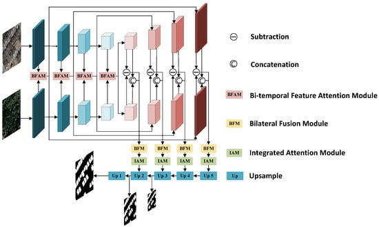
Figure 1.
General overview of AMFNet.
2.1.2. Bi-Temporal Feature Attention Module
In the change detection model, bi-temporal feature fusion involves operator fusion methods, convolution fusion methods, and attention fusion methods. Simple operator fusion methods directly add, subtract, or concatenate bi-temporal features for fusion [54,55,56]. However, noise in bi-temporal features might easily interfere with obtaining reliable detection results using these methods. Convolutional fusion methods enhance bi-temporal features in terms of multi-scale and semantic hierarchies through various convolution operations, reducing the noise interference on bi-temporal features [57]. Typically, the attention fusion approaches use an attention mechanism to effectively fuse bi-temporal characteristics in the channel and spatial dimensions. Convolutional methods concentrate on enhancing bi-temporal characteristics before fusion, while attention refinement approaches focus on improving these characteristics after operator fusion. The temporal information of bi-temporal characteristics is disregarded by both.
As illustrated in Figure 2, we propose a bi-temporal feature attention model (BFAM) to address the problems mentioned previously. BFAM effectively fuses features by utilizing temporal information. The significant portions of the characteristics are identified using channel and spatial attention, and the key sections between the bi-temporal features are identified using temporal information. The channel branch achieves the aggregate of channel information by transmitting the input bi-temporal characteristics across channels via global pooling. The aggregation process can be represented as follows:
where represents the fused channel features. denotes concatenation in the channel dimension. Global average pooling is represented by , and global maximum pooling by . and are the bi-temporal feature inputs. The fused channel features are then passed through one-dimensional convolutions separately with adaptively determined kernel numbers (k), effectively capturing dependencies between channels. This is followed by the generation of attention weights and for the channels using a nonlinear activation function, softmax. The formulation of the two channel weights can be expressed as follows:
where and represent one-dimensional convolution. The methodology for determining the weights in the spatial dimension parallels that of the channel dimension. Global pooling is applied in the spatial dimension, and weights are obtained using two-dimensional convolution and a nonlinear activation function. In the spatial branch, we identify specific regions between bi-temporal characteristics by calculating the bi-temporal spatial weights and . By integrating bi-temporal channel weights and bi-temporal spatial weights, comprehensive bi-temporal weights are obtained, highlighting the essential parts among bi-temporal features. Subsequently, these bi-temporal weights are multiplied with the bi-temporal features for an effective fusion of these features. The resulting output is processed through a convolution and a depth-wise separable convolution, characterized by a lower parameter count, and is then summed with the original input. The output can be formalized as follows:
where represents a set of convolutions, batch normalization, and ReLU activation functions, and stands for depth-wise separable convolution [58], which encompasses depth-wise convolution and point-wise convolution. ⊗ stands for the multiplication operation. This approach significantly reduces the number of parameters while ensuring a larger receptive field.
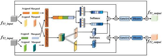
Figure 2.
Bi-temporal feature attention module.
2.1.3. Bilateral Fusion Module
In change detection, the commonly used methods for extracting change information involve addition, subtraction, and concatenation operations [47]. However, these simple operator operations for extracting change features often lead to redundant information, significantly reducing the robustness of change detection. Moreover, deep-level semantic information in the network is abstract, and direct simple operations can result in misjudgments and omissions [59]. To reasonably utilize the difference information and global information generated from the subtraction and concatenation of bi-temporal feature maps, we propose a BFM module, as shown in Figure 3. This module aims to precisely locate changed positions from the abstract bi-temporal feature information in the deep network, further revealing details and texture features of the changes.
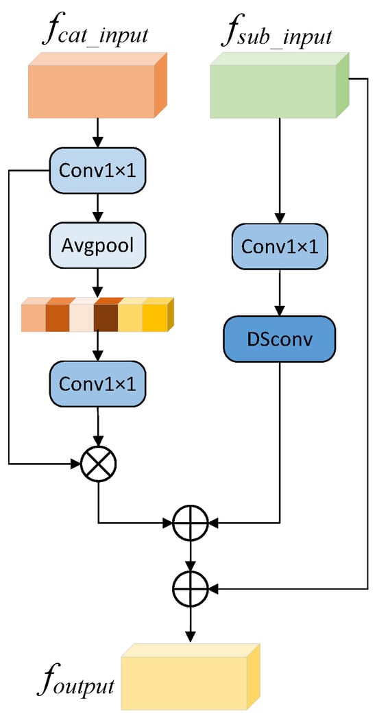
Figure 3.
Bilateral fusion module.
Two branches make up the module: the right branch for extracting difference information and the left branch for extracting global information. Since the initial difference information is obtained by subtracting bi-temporal feature maps, the size of is . It is then processed through a convolution and a depth-wise separable convolution [58] to further extract difference features. For the left branch, the initial global information is obtained by concatenating bi-temporal feature maps along the channel dimension, resulting in with a size of . It first passes through a convolution to obtain an output of size and then undergoes global average pooling to obtain a feature map of size . After further extracting features through a convolution from the weight feature map, it is multiplied by the feature map of size before global pooling to obtain more accurate global information. The ultimate output, , is obtained by fusing the characteristics of the two branches and adding the result to .
Through a sequence of convolution and pooling procedures, the module better extracts change features. The use of a residual structure guides the difference between information and global information, which mutually influence each other, resulting in finer granularity in extracting the edges of change regions. The following are the mathematical expressions:
2.1.4. Integrated Attention Module
Remote sensing images, especially high-resolution ones, frequently encompass extensive data volumes and intricate content details. However, our focus is on the change information between bi-temporal images, primarily including buildings, vegetation, rivers, and infrastructure [55]. The characteristics of the changed targets are often not obvious [40], and the complex background interferes with the target areas [25]. For each pixel label, it is challenging for the network to classify and recognize correctly, which may lead to misjudgment and omission of target features. Considering that unidirectional axial attention may result in the omission of feature information in other dimensions, we propose a novel attention mechanism module, IAM, which consists of two branches. The first branch guides the initial features, while the second branch integrates spatial attention and channel attention mechanisms, enabling simultaneous focus on channel and spatial change information. The two branches employ skip connections for feature fusion, facilitating mutual guidance between the branches. This adaptive attention mechanism allows for more attention to be placed on the changing areas, highlighting their importance while suppressing the non-changing regions. The output is more refined attention features, with a greater focus on the details of the edges in the changing areas. The structure of this module is displayed in Figure 4.

Figure 4.
Integrated attention module.
Suppose that input , where H and W denote the feature map’s height and width, respectively, while C signifies the quantity of channels involved. Initially, the input features are subjected to channel dimension weight resetting by CAM, which involves spatial axis operations on features under each channel. The structure of CAM is illustrated in Figure 5. Specifically, this means condensing the feature map into two vectors of size by executing both spatial plane max pooling and global average pooling. These two vectors are then input separately into a multi-layer perceptron (MLP) in order to perform classification. The channel attention weights (where D is the feature dimension and d is the dth feature) are calculated by integrating the MLP outputs and passing them through a sigmoid activation function. These weights also have the size of . Each element of this vector represents the receptive field of the corresponding channel space. The weighted fusion of the channel attention weights and the input feature map results in the process of refining input features in the channel. This reduces unnecessary channels and highlights those that are important for change detection. The computational formula for the above process can be described as follows:
where represents sigmoid activation function. represents multi-layer perceptron operation. and represent global average pooling and global maximum pooling, respectively.

Figure 5.
Channel attention module.
SAM begins by applying AvgPool and MaxPool operations along the channel axis to the feature map . The structure of SAM is shown in Figure 6. This compression of channel information produces two tensors of size . These tensors are then concatenated and processed through two consecutive convolution operations, which flexibly construct spatial relationships of features. This convolutional operation is equivalent to the receptive field of a convolution but with a significantly reduced parameter count. Finally, a sigmoid activation function is introduced to enhance its nonlinear expression, resulting in the spatial attention weight map , where N represents the total number of pixels in each feature map and p denotes the value of the pth pixel in the attention map. Higher and lower weights are, respectively, allocated to pixels that have changed and those that have not changed. The input feature map is multiplied element-wise by each element in . Pixels within changing regions are multiplied by higher weights, while pixels within unchanged areas are suppressed by lower weights, achieving spatial refinement. This enables the network to rapidly detect areas undergoing change. The computation formula is as follows:
where symbolizes a two-dimensional convolution, inclusive of batch normalization and a ReLU activation function, characterized by a 3-unit convolution kernel. denotes the operation of concatenation along the channel dimension. Meanwhile, is indicative of a feature map that has been enhanced through the use of SAM. and the original input undergo a series of multiplication and fusion operations, enhancing feature selection and preserving important information. The concatenated feature map is then passed through a convolutional layer with a kernel size of . Lastly, the final output feature map, , is obtained by adding the output element-by-element to the original feature map. The formula for the process is specified as follows:

Figure 6.
Spatial attention module.
2.2. Datasets
In order to thoroughly confirm the validity of our AMFNet model, we assessed its capability using three distinct remote sensing image change detection datasets: SYSU-CD [60], LEVIR-CD [43], and GZ-CD [61].
2.2.1. SYSU-CD
Sun Yat-sen University created and released the SYSU-CD dataset [60] in 2022, which is a collection of datasets created especially for change detection applications. This dataset is primarily focused on detecting changes in various natural elements. The dataset comprises distinct sets for training, validating, and testing purposes. It is methodically divided in a ratio of 6:2:2, with 12,000 images allocated for training, 4000 for validation, and another 4000 for testing, ensuring comprehensive coverage for machine learning applications. Each image within the dataset maintains a standard resolution of 256 × 256 pixels, suitable for detailed analysis. Figure 7 displays some example.
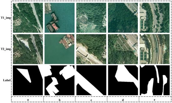
Figure 7.
Diagram of the SYSU-CD dataset. (a–e) correspond to example images in the dataset.
2.2.2. LEVIR-CD
Including very high-quality Google Earth pictures, the LEVIR-CD [43] dataset is a large-scale change detection dataset. The dataset spans a timeframe of 5 to 14 years, with the images captured between 2002 and 2018 primarily focusing on significant transformations in building structures. It includes bi-temporal remote sensing images from 20 distinct areas across multiple cities in Texas, encompassing a wide array of buildings like villas, skyscrapers, small garages, and large warehouses. This diverse collection takes into consideration changes due to seasonal shifts and varying light conditions. For practical applications, the images are resized to 256 × 256 pixels. Using a 7:1:2 ratio, the dataset is logically split into training, validation, and test sets containing 7120, 1024, and 2048 picture pairings, respectively. The data structure is depicted in Figure 8.
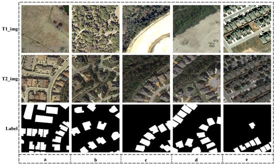
Figure 8.
Diagram of the LEVIR-CD dataset. (a–e) correspond to example images in the dataset.
2.2.3. GZ-CD
The GZ-CD dataset [61], obtained from a suburban area of Guangzhou, China, captures the rapid urban development experienced during its collection, including various alterations in the architecture’s shape and size. It showcases a rich diversity of building types, ranging from expansive industrial facilities to compact mobile homes. Given that the bi-temporal images in this dataset maintain consistent resolution, they were specifically utilized for resolution-independent difference experiments within this methodology to evaluate the model’s adaptability and generalization skills. Figure 9 displays some examples.
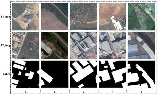
Figure 9.
Diagram of the GZ-CD dataset. (a–e) correspond to example images in the dataset.
2.3. Implementation Details
2.3.1. Evaluation Metrics
To evaluate the performance of our AMFNet model in change detection tasks, we utilized a comprehensive set of evaluation metrics, including precision (), recall (), overall accuracy (), Kappa coefficient (), intersection over union ), and F1 score (). These metrics collectively offer a detailed assessment of the model. The primary indicators used for evaluation are the F1 score, which measures the accuracy of the changed category, and the , assessing the overlap between predicted and actual changed areas. Additionally, , , , and serve as supporting indicators, enriching the evaluation by providing insights into various aspects of the model’s accuracy and reliability. The calculation method of each index is as follows:
In the formulas mentioned above, denotes the true positive, which corresponds to the area of change predicted correctly; signifies the false positive, representing the unchanged area mistakenly identified as changed; is the true negative, referring to the area that is correctly identified as unchanged; indicates the false negative, which is the area of change incorrectly labeled as unchanged.
2.3.2. Multi-Scale Deep Supervised Training
To assist the network in better learning useful feature representations and to accelerate the training process, we incorporate additional loss functions at multiple intermediate layers of the network for multi-scale supervision [52,62]. Changes in change detection tasks can occur at various scales, from large-scale geographical or architectural changes to minor object movements or alterations. Multi-scale supervision ensures that the network effectively learns features at all scales, thereby enhancing its ability to detect changes across different scales. The goal of multi-scale supervision training is to minimize the following:
For losses at different levels, we sequentially define them as , , and from shallow to deep layers. and represent the weights of auxiliary losses at different scales, respectively. We use shallow layer losses as a baseline because shallow layers are usually able to capture more details and texture information, which is crucial for change detection tasks. Moreover, features in shallow layers are closer to the input data, making the loss calculation potentially more stable.
3. Experiment and Results
In this part, we use the GZ-CD, SYSU-CD, and LEVIR-CD datasets for ablation studies and comparison experiments to thoroughly assess the performance of our proposed network and components.
3.1. Experimental Details
The research was conducted using a GeForce RTX 4090 GPU manufactured by NVIDIA, with the chip produced in Taiwan, China, and employed PyTorch (version 2.1) with CUDA 12.1 as the foundational framework. During training, the batch size was established at six, with an initial learning rate () of 0.0001. This learning rate is subject to dynamic modification, adhering to a polynomial adjustment strategy. The computational expression for this adjustment is detailed as follows:
The new learning rate, denoted as , is calculated from the initial learning rate , taking into account the current iteration number (), the maximum iteration number (), and a constant p that controls the decay rate. The epoch count is fixed at 200. Moreover, the network employs binary cross-entropy loss as its loss function and utilizes the Adam optimization algorithm.
3.2. Ablation Experiments on LEVIR-CD
Selecting the right backbone network is crucial for our experiments. We considered ResNet18, ResNet34, ResNet50, VGG16, and VGG19. Table 1, highlighting the best results in bold, indicates ResNet34’s superior performance.

Table 1.
Comparative experiments of AMFNet under different backbone networks (best results are highlighted in bold type).
By adding or removing modules, we examine the function of each component in order to comprehend complicated neural networks. We use the LEVIR-CD dataset for ablation studies to assess these modules’ performance on the backbone network. To directly view the effectiveness of the model, we focus on the PR (precision), RC (recall), IoU (ontersection over union), and metrics. The details are exhibited in Table 2.

Table 2.
The assessment of our proposed module through ablative experiments (best results are highlighted in bold type).
- Ablation experiments of BFAM: We propose the attention-guided BFAM module, which effectively incorporates temporal dynamics into the feature fusion process at both channel and spatial dimensions. This module enhances IoU and F1 scores by 0.78% and 1.13 %, respectively, validating the effectiveness of the proposed module. Table 3 shows the ablation experiment of the convolution kernel size k used for one-dimensional convolution at the channel latitude. The experiment proves that the model performs best when k is an adaptive channel size. From heatmap2 in Figure 10, it can be observed that, compared to heatmap1, the addition of BFAM significantly reduces the areas of misjudgment. The weights along the edges of the target buildings become more pronounced, leading to a more precise localization of the edges.
 Table 3. Ablation experiment of one-dimensional convolution kernel of channel latitude in BFAM (best results are highlighted in bold type).
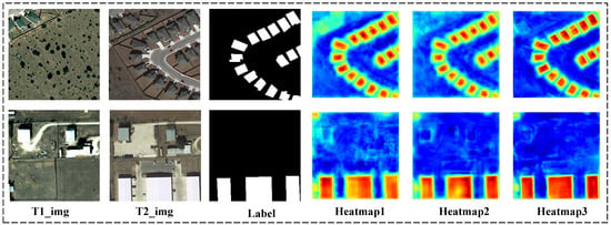 Figure 10. Heatmaps depicting the ablation of different modules. Heatmap1 represents the heatmap of the backbone network, Heatmap2 is the heatmap after adding the BFAM module, and Heatmap3 is the heatmap after adding the BFAM, BFM, and IAM modules.
 - Ablation experiments of BFM: Our proposed BFM facilitates the network in precisely identifying changing locations during the feature decoding phase by integrating global and differential information, thereby enhancing the representation of texture and edge features. Experimental results shown in Table 2 demonstrate that BFM successfully integrates two semantic pieces of information, improving the MIoU score by 0.60% and the F1 score by 0.37%, enhancing the model’s accuracy.
- Ablation experiments of IAM: The attention module enables the network to adaptively adjust the weights and pixel positions across each channel, emphasizing factors related to changes while suppressing irrelevant ones. This method is a crucial approach to improving feature extraction efficiency in the network. The experimental findings presented in Table 2 show that AMFNet raises the F1 score by 0.31% and the IoU by 0.52%, affirming the accuracy of the proposed module. From Heatmap3 in Figure 10, it is evident that employing interactive features for decoding, a key innovation in this paper, achieves remarkable results. The decoded feature maps undergo further processing through BFM and IAM, leading to a higher emphasis on the target regions. This results in a reduction of misjudgments and omissions along the edges, making the distinction between changed and unchanged regions more apparent.
- Ablation experiments of multi-scale supervised training: In order to enhance the detection capability of changes at various scales, we add losses from different layers in the decoding stage to the overall training loss in a certain proportion. This results in an improvement of 0.40% and 0.78% in the F1 and IoU scores, respectively, strengthening the model’s robustness.
Table 4 presents the ablation experiment results of BFAM and IAM on the LEVIR-CD dataset. Both modules are attention-guided fusion modules, with BFAM fusing multi-scale bi-temporal feature maps in the encoding stage and IAM highlighting changing regions and suppressing non-changing regions in the decoding stage. For comparison, we selected CBAM [63] as a conventional attention mechanism model. The first and second rows indicate that using BFAM allows concentrating on the more critical aspects between bi-temporal features in the encoding stage, effectively fusing the bi-temporal features, thereby improving performance. The data in the first and third rows suggest that relative to conventional attention models, employing IAM enhances the merging of multi-semantic features during the decoding phase, thus boosting performance. The fourth row shows that using both BFAM and IAM simultaneously can further enhance performance. According to the data above, change detection capabilities may be further enhanced by integrating BFAM and IAM, which together can boost performance even more.

Table 4.
Attention-guided module ablation experiments (best results are highlighted in bold type).
3.3. Comparative Experiments with Other Classical Networks
3.3.1. Comparative Experiments of Different Algorithms on LEVIR-CD
To fully comprehend and analyze the performance of our model, we contrasted it with many models. Every method applied the same training approach to guarantee comparative fairness, ensuring reliable results. The specific quantified results of various model evaluation metrics are listed in Table 5. Params (M) represents the total number of trainable parameters in the model, expressed in millions, indicating the model’s complexity and capacity. FLOPs (G) denotes the number of floating-point operations required to run the model once, measured in billions, reflecting the computational cost. Time (ms) measures the time taken to execute one forward pass of the model in milliseconds, providing a direct metric of the model’s inference speed. From the comparative experimental results, it is evident that among the change detection methods using deep learning, FC-EF performs the worst, with F1 and IoU scores of only 83.17% and 71.19%, respectively. In contrast, AMFNet demonstrated increases of 0.69% in F1 score and 1.15% in IoU, alongside notable improvements in precision (+2.98%), recall (+2.39%), Kappa (+0.72%), and overall accuracy (+0.05%). Our approach exceeds other algorithms in terms of overall performance based on many measures, which is a clear indication of its potential superiority in practical applications.

Table 5.
Comparative experiments on the LEVIR-CD dataset (best results are highlighted in bold type).
To visualize the prediction results, Figure 11 displays the predicted maps of different algorithms on the LEVIR-CD dataset. We selected three sets of different remote sensing images and generated prediction maps, further illustrating that our algorithm outperforms other state-of-the-art algorithms. Here, white indicates true positives, black indicates true negatives, red indicates false positives, and green indicates false negatives. From the prediction results of the three sets of comparative experiments, it can be observed that other change detection models exhibit more severe omissions and exaggerations, especially in areas with similar features such as color and lighting. In contrast, our proposed algorithm performs better in detecting small-area and high-similarity change regions, providing more accurate predictions of edge details.
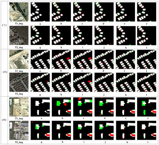
Figure 11.
Three groups of comparative diagrams illustrating the performance of different algorithms on the LEVIR-CD dataset. (a–l) corresponds to the predicted maps of labels, FC-EF, FC-Siam-Conc, FC-Siam-Diff, ChangNet, DSIFN, BIT, ICFNet, SNUNet, DMINet, SAGNet, and our AMFNet network.
3.3.2. Comparative Experiments of Different Algorithms on GZ-CD
We ran comparison tests on the GZ-CD dataset to confirm the effectiveness of our AMFNet method. The outcomes are shown in Table 6. It is evident from the F1 and IoU scores that FC-Siam-Diff performs the worst, with F1 and IoU scores of only 71.06% and 55.11%, respectively. The remaining change detection algorithms show improvements in all four metrics, with our AMFNet exhibiting the best performance. F1 and IoU scores reached 88.09% and 69.85%, respectively, which are 1.79% and 2.80% higher than the second-ranked SAGNet, indicating excellent generalization ability and robustness of our algorithm.

Table 6.
Comparative experiments on the GZ-CD dataset (best results are highlighted in bold type).
On the GZ-CD dataset, the predicted maps for each comparative experiment are illustrated in Figure 12. Other change detection algorithms often exhibit extensive misjudgments and omissions at the edges of change regions. In contrast, our proposed algorithm achieves more accurate edge detection and demonstrates stronger detection capabilities for small targets similar to the background. In Figure 12(II), the portion enclosed by the three buildings on the right side of the image remains unchanged and is still land. However, due to external environmental changes such as lighting and seasonality, many algorithms misclassify it as a changed area. Our algorithm accurately identifies this as an unchanged area, proving the effectiveness of our AMFNet algorithm in change detection tasks.
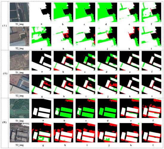
Figure 12.
Three groups of comparison diagrams of different algorithms on GZ-CD dataset. (a–l) corresponds to the predicted maps of labels, FC-EF, FC-Siam-Conc, FC-Siam-Diff, ChangNet, DSIFN, BIT, ICFNet, SNUNet, DMINet, SAGNet, and our AMFNet network.
3.3.3. Comparative Experiments of Different Algorithms on SYSU-CD
Concerning the SYSU-CD dataset, our model AMFNet achieved the highest IoU and F1 indicators, reaching 69.85% and 82.25%, respectively. The outcomes are shown in Table 7.

Table 7.
Comparative experiments on the SYSU-CD dataset (best results are highlighted in bold type).
Figure 13 illustrates the prediction results of different algorithms on the SYSU-CD dataset. Notably, in Figure 13(II), the bottom-right corner contains a shadow, and the outlines of the buildings are somewhat blurred, posing a significant challenge to the change detection task. Other change detection algorithms perform poorly in this region, resulting in numerous misjudgments. In contrast, our proposed algorithm accurately identifies changes in this part. From Figure 13, it is evident that the AMFNet algorithm achieves more precise edge detection and can effectively extract image features for accurate judgment even in challenging environments. It demonstrates robustness in situations where the target area is highly similar to the background.
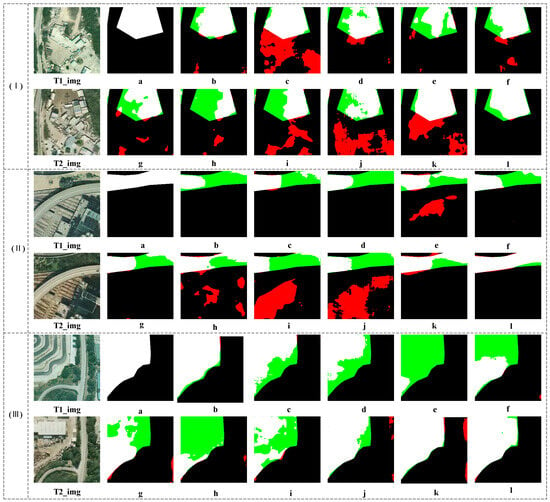
Figure 13.
Three groups of comparative diagrams illustrating the performance of different algorithms on the SYSU-CD dataset. (a–l) corresponds to the predicted maps of labels, FC-EF, FC-Siam-Conc, FC-Siam-Diff, ChangNet, DSIFN, BIT, ICFNet, SNUNet, DMINet, SAGNet, and our AMFNet network.
4. Discussion
4.1. Advantages of the Proposed Method
The proposed attention-guided multi-scale fusion network (AMFNet) introduces significant advancements in the field of change detection. By integrating the bi-temporal feature attention module (BFAM), AMFNet effectively manages the interaction of bi-temporal features, reducing redundancy and enhancing the perception of changes over time. This is a crucial improvement over traditional methods that rely merely on simple arithmetic operations. The incorporation of the bi-temporal fusion module (BFM) in the decoder further refines the process by selectively fusing semantic information, which significantly reduces the intrusion of irrelevant data. Furthermore, the innovative use of the interactive attention module (IAM) in the decoding process not only preserves the temporal sequence but also emphasizes the importance of non-local relationships, allowing for a more nuanced understanding of the scene dynamics. These methodological enhancements enable AMFNet to achieve superior performance metrics, as evidenced by its high F1 scores and intersection over union (IoU) metrics across multiple datasets.
4.2. Limitations and Expectations
While the proposed AMFNet demonstrates impressive performance, it is not without its limitations. The complexity introduced by attention mechanisms and multiscale fusion could lead to increased computational demands [70], potentially hindering real-time processing capabilities or deployment in computationally constrained environments [71]. The model’s sensitivity to hyperparameters and network architecture choices also poses a challenge, necessitating careful tuning to achieve the best possible performance. Furthermore, the current evaluation of the model’s effectiveness has been limited to specific datasets, and its adaptability to larger-scale remote sensing images with more diverse regions [69] remains uncertain. Looking ahead, it is essential to concentrate research efforts on enhancing computational efficiency, reducing the model’s sensitivity to parameter settings, and improving scalability. Such advancements will be crucial in extending the applicability of AMFNet to a wider array of real-world scenarios, thereby solidifying its position as a robust tool in the realm of remote sensing and change detection.
5. Conclusions
In this paper, we proposed an attention-guided multiscale fusion network. The traditional change detection algorithm simply adds and subtracts bi-temporal features, which have a large amount of redundant information and insufficient perception of the tense. So, in the encoding part, we utilized BFAM to facilitate the interaction of bi-temporal features at the same level, eliminating redundant information. Our decoding process was based on interactive feature maps, preserving both the temporal sequence and rich non-local relationships of bi-temporal features during further fusion. By incorporating BFM into the decoder network to fuse global semantic and differential semantic information, we avoided introducing a significant amount of irrelevant semantic information through simple fusion methods. By assigning weights adaptively to different regions, the IAM sharpened the network’s emphasis on differentiating targets from backgrounds and enhances its capacity to identify tiny objects and edge features. Our proposed AMFNet outperforms existing algorithms on the LEVIR-CD, GZ-CD, and SYSU-CD datasets, according to experimental findings. Specifically, it achieved F1 scores of 90.79%, 88.09%, and 82.25%, and IoU metrics of 83.13%, 78.71%, and 69.85% for each dataset, respectively. The model exhibited excellent generalization and robustness.
Author Contributions
Conceptualization, Z.Z. and M.X.; methodology, M.X. and H.R.; software, Z.Z.; validation, X.L., X.W., M.X. and H.L.; formal analysis, M.X.; investigation, Z.Z.; resources, M.X. and H.R.; data curation, Z.Z.; writing—original draft preparation, Z.Z.; writing—review and editing, X.W. and M.X.; visualization, Z.Z.; supervision, M.X.; project administration, M.X.; funding acquisition, M.X. All authors have read and agreed to the published version of the manuscript.
Funding
This work was supported, in part, by the National Natural Science Foundation of PR China (42075130).
Data Availability Statement
The data and the code of this study are available from the corresponding author upon request.
Conflicts of Interest
The authors declare no conflicts of interest.
References
- Amare, M.T.; Demissie, S.T.; Beza, S.A.; Erena, S.H. Land cover change detection and prediction in the Fafan catchment of Ethiopia. J. Geovis. Spat. Anal. 2023, 7, 19. [Google Scholar] [CrossRef]
- Eisavi, V.; Homayouni, S.; Karami, J. Integration of remotely sensed spatial and spectral information for change detection using FAHP. J. Fac. For. Istanb. Univ. 2016, 66, 524–538. [Google Scholar] [CrossRef]
- de Alwis Pitts, D.A.; So, E. Enhanced change detection index for disaster response, recovery assessment and monitoring of accessibility and open spaces (camp sites). Int. J. Appl. Earth Obs. Geoinf. 2017, 57, 49–60. [Google Scholar] [CrossRef]
- Tan, K.; Ma, W.; Chen, L.; Wang, H.; Du, Q.; Du, P.; Yan, B.; Liu, R.; Li, H. Estimating the distribution trend of soil heavy metals in mining area from HyMap airborne hyperspectral imagery based on ensemble learning. J. Hazard. Mater. 2021, 401, 123288. [Google Scholar] [CrossRef]
- Qin, H.; Wang, J.; Mao, X.; Zhao, Z.; Gao, X.; Lu, W. An Improved Faster R-CNN Method for Landslide Detection in Remote Sensing Images. J. Geovis. Spat. Anal. 2024, 8, 2. [Google Scholar] [CrossRef]
- Ji, R.; Tan, K.; Wang, X.; Pan, C.; Xin, L. Spatiotemporal monitoring of a grassland ecosystem and its net primary production using Google Earth Engine: A case study of inner mongolia from 2000 to 2020. Remote Sens. 2021, 13, 4480. [Google Scholar] [CrossRef]
- Kokila, S.; Jayachandran, A. Hybrid Behrens-Fisher-and gray contrast–based feature point selection for building detection from satellite images. J. Geovis. Spat. Anal. 2023, 7, 8. [Google Scholar] [CrossRef]
- Wang, Z.; Xia, M.; Weng, L.; Hu, K.; Lin, H. Dual Encoder–Decoder Network for Land Cover Segmentation of Remote Sensing Image. IEEE J. Sel. Top. Appl. Earth Obs. Remote Sens. 2024, 17, 2372–2385. [Google Scholar] [CrossRef]
- Weismiller, R.; Kristof, S.; Scholz, D.; Anuta, P.; Momin, S. Change detection in coastal zone environments. Photogramm. Eng. Remote Sens. 1977, 43, 1533–1539. [Google Scholar]
- Ke, L.; Lin, Y.; Zeng, Z.; Zhang, L.; Meng, L. Adaptive Change Detection With Significance Test. IEEE Access 2018, 6, 27442–27450. [Google Scholar] [CrossRef]
- Rignot, E.J.; Van Zyl, J.J. Change detection techniques for ERS-1 SAR data. IEEE Trans. Geosci. Remote Sens. 1993, 31, 896–906. [Google Scholar] [CrossRef]
- Ridd, M.K.; Liu, J. A comparison of four algorithms for change detection in an urban environment. Remote Sens. Environ. 1998, 63, 95–100. [Google Scholar] [CrossRef]
- Ferraris, V.; Dobigeon, N.; Wei, Q.; Chabert, M. Detecting changes between optical images of different spatial and spectral resolutions: A fusion-based approach. IEEE Trans. Geosci. Remote Sens. 2017, 56, 1566–1578. [Google Scholar] [CrossRef]
- Du, P.; Wang, X.; Chen, D.; Liu, S.; Lin, C.; Meng, Y. An improved change detection approach using tri-temporal logic-verified change vector analysis. ISPRS J. Photogramm. Remote Sens. 2020, 161, 278–293. [Google Scholar] [CrossRef]
- Deng, J.; Wang, K.; Deng, Y.; Qi, G. PCA-based land-use change detection and analysis using multitemporal and multisensor satellite data. Int. J. Remote Sens. 2008, 29, 4823–4838. [Google Scholar] [CrossRef]
- Zhang, X.; Yang, P.; Zhou, M. Multireceiver SAS imagery with generalized PCA. IEEE Geosci. Remote Sens. Lett. 2023, 20, 1502205. [Google Scholar] [CrossRef]
- Raj, J.R.; Srinivasulu, S. Change detection of images based on multivariate alteration detection method. In Proceedings of the 2020 6th International Conference on Advanced Computing and Communication Systems (ICACCS), Coimbatore, India, 6–7 March 2020; pp. 847–850. [Google Scholar]
- Chen, H.; Yokoya, N.; Chini, M. Fourier domain structural relationship analysis for unsupervised multimodal change detection. ISPRS J. Photogramm. Remote Sens. 2023, 198, 99–114. [Google Scholar] [CrossRef]
- Ji, L.; Zhao, J.; Zhao, Z. A Novel End-to-End Unsupervised Change Detection Method with Self-Adaptive Superpixel Segmentation for SAR Images. Remote Sens. 2023, 15, 1724. [Google Scholar] [CrossRef]
- Dou, P.; Han, Z. Quantifying Land Use/Land Cover Change and Urban Expansion in Dongguan, China, From 1987 to 2020. IEEE J. Sel. Top. Appl. Earth Obs. Remote Sens. 2022, 15, 201–209. [Google Scholar] [CrossRef]
- Dou, P.; Chen, Y. Dynamic monitoring of land-use/land-cover change and urban expansion in Shenzhen using Landsat imagery from 1988 to 2015. Int. J. Remote Sens. 2017, 38, 5388–5407. [Google Scholar] [CrossRef]
- Juan, S.; Gui-Jin, W.; Xing-Gang, L.; Dai-Zhi, L. A change detection algorithm for man-made objects based on multi-temporal remote sensing images. Acta Autom. Sin. 2008, 34, 1040–1046. [Google Scholar]
- Wan, L.; Xiang, Y.; You, H. A post-classification comparison method for SAR and optical images change detection. IEEE Geosci. Remote Sens. Lett. 2019, 16, 1026–1030. [Google Scholar] [CrossRef]
- Wang, X.; Girshick, R.; Gupta, A.; He, K. Non-local neural networks. In Proceedings of the IEEE Conference on Computer Vision and Pattern Recognition, Salt Lake City, UT, USA, 18–23 June 2018; pp. 7794–7803. [Google Scholar]
- Wu, C.; Du, B.; Cui, X.; Zhang, L. A post-classification change detection method based on iterative slow feature analysis and Bayesian soft fusion. Remote Sens. Environ. 2017, 199, 241–255. [Google Scholar] [CrossRef]
- Tan, K.; Zhang, Y.; Wang, X.; Chen, Y. Object-based change detection using multiple classifiers and multi-scale uncertainty analysis. Remote Sens. 2019, 11, 359. [Google Scholar] [CrossRef]
- Han, Y.; Javed, A.; Jung, S.; Liu, S. Object-based change detection of very high resolution images by fusing pixel-based change detection results using weighted Dempster–Shafer theory. Remote Sens. 2020, 12, 983. [Google Scholar] [CrossRef]
- Dou, P.; Huang, C.; Han, W.; Hou, J.; Zhang, Y.; Gu, J. Remote sensing image classification using an ensemble framework without multiple classifiers. ISPRS J. Photogramm. Remote Sens. 2024, 208, 190–209. [Google Scholar] [CrossRef]
- Jiang, S.; Dong, R.; Wang, J.; Xia, M. Credit Card Fraud Detection Based on Unsupervised Attentional Anomaly Detection Network. Systems 2023, 11, 305. [Google Scholar] [CrossRef]
- Dou, P.; Shen, H.; Li, Z.; Guan, X. Time series remote sensing image classification framework using combination of deep learning and multiple classifiers system. Int. J. Appl. Earth Obs. Geoinf. 2021, 103, 102477. [Google Scholar] [CrossRef]
- Dai, X.; Chen, K.; Xia, M.; Weng, L.; Lin, H. LPMSNet: Location Pooling Multi-Scale Network for Cloud and Cloud Shadow Segmentation. Remote Sens. 2023, 15, 4005. [Google Scholar] [CrossRef]
- Wang, X.; Yan, X.; Tan, K.; Pan, C.; Ding, J.; Liu, Z.; Dong, X. Double U-Net (W-Net): A change detection network with two heads for remote sensing imagery. Int. J. Appl. Earth Obs. Geoinf. 2023, 122, 103456. [Google Scholar] [CrossRef]
- Chen, K.; Dai, X.; Xia, M.; Weng, L.; Hu, K.; Lin, H. MSFANet: Multi-Scale Strip Feature Attention Network for Cloud and Cloud Shadow Segmentation. Remote Sens. 2023, 15, 4853. [Google Scholar] [CrossRef]
- Ding, L.; Xia, M.; Lin, H.; Hu, K. Multi-Level Attention Interactive Network for Cloud and Snow Detection Segmentation. Remote Sens. 2024, 16, 112. [Google Scholar] [CrossRef]
- Weng, L.; Pang, K.; Xia, M.; Lin, H.; Qian, M.; Zhu, C. Sgformer: A Local and Global Features Coupling Network for Semantic Segmentation of Land Cover. IEEE J. Sel. Top. Appl. Earth Obs. Remote Sens. 2023, 16, 6812–6824. [Google Scholar] [CrossRef]
- Niu, C.; Tan, K.; Jia, X.; Wang, X. Deep learning based regression for optically inactive inland water quality parameter estimation using airborne hyperspectral imagery. Environ. Pollut. 2021, 286, 117534. [Google Scholar] [CrossRef] [PubMed]
- Ji, H.; Xia, M.; Zhang, D.; Lin, H. Multi-Supervised Feature Fusion Attention Network for Clouds and Shadows Detection. ISPRS Int. J. Geo-Inf. 2023, 12, 247. [Google Scholar] [CrossRef]
- Long, J.; Shelhamer, E.; Darrell, T. Fully convolutional networks for semantic segmentation. In Proceedings of the IEEE Conference on Computer Vision and Pattern Recognition, Boston, MA, USA, 7–12 June 2015; pp. 3431–3440. [Google Scholar]
- Li, X.; He, M.; Li, H.; Shen, H. A combined loss-based multiscale fully convolutional network for high-resolution remote sensing image change detection. IEEE Geosci. Remote Sens. Lett. 2021, 19, 8017505. [Google Scholar] [CrossRef]
- Ronneberger, O.; Fischer, P.; Brox, T. U-net: Convolutional networks for biomedical image segmentation. In Proceedings of the Medical Image Computing and Computer-Assisted Intervention–MICCAI 2015: 18th International Conference, Munich, Germany, 5–9 October 2015; Proceedings, Part III 18. Springer: Berlin/Heidelberg, Germany, 2015; pp. 234–241. [Google Scholar]
- Chen, H.; Qi, Z.; Shi, Z. Remote sensing image change detection with transformers. IEEE Trans. Geosci. Remote Sens. 2021, 60, 5900318. [Google Scholar] [CrossRef]
- Xing, Y.; Jiang, J.; Xiang, J.; Yan, E.; Song, Y.; Mo, D. LightCDNet: Lightweight Change Detection Network Based on VHR Images. IEEE Geosci. Remote Sens. Lett. 2023, 20, 2504105. [Google Scholar] [CrossRef]
- Chen, H.; Shi, Z. A spatial-temporal attention-based method and a new dataset for remote sensing image change detection. Remote Sens. 2020, 12, 1662. [Google Scholar] [CrossRef]
- Lv, Z.; Huang, H.; Sun, W.; Lei, T.; Benediktsson, J.A.; Li, J. Novel enhanced UNet for change detection using multimodal remote sensing image. IEEE Geosci. Remote Sens. Lett. 2023, 20, 2505405. [Google Scholar] [CrossRef]
- Lv, Z.; Liu, J.; Sun, W.; Lei, T.; Benediktsson, J.A.; Jia, X. Hierarchical attention feature fusion-based network for land cover change detection with homogeneous and heterogeneous remote sensing images. IEEE Trans. Geosci. Remote Sens. 2023, 61, 4411115. [Google Scholar] [CrossRef]
- Lv, Z.; Zhang, P.; Sun, W.; Lei, T.; Benediktsson, J.A.; Li, P. Sample Iterative Enhancement Approach for Improving Classification Performance of Hyperspectral Imagery. IEEE Geosci. Remote Sens. Lett. 2023, 21, 2500605. [Google Scholar] [CrossRef]
- Ren, H.; Xia, M.; Weng, L.; Hu, K.; Lin, H. Dual-Attention-Guided Multiscale Feature Aggregation Network for Remote Sensing Image Change Detection. IEEE J. Sel. Top. Appl. Earth Obs. Remote Sens. 2024, 17, 4899–4916. [Google Scholar] [CrossRef]
- Song, L.; Xia, M.; Jin, J.; Qian, M.; Zhang, Y. SUACDNet: Attentional change detection network based on siamese U-shaped structure. Int. J. Appl. Earth Obs. Geoinf. 2021, 105, 102597. [Google Scholar] [CrossRef]
- Luo, F.; Zhou, T.; Liu, J.; Guo, T.; Gong, X.; Ren, J. Multiscale diff-changed feature fusion network for hyperspectral image change detection. IEEE Trans. Geosci. Remote Sens. 2023, 61, 5502713. [Google Scholar] [CrossRef]
- Wang, Y.; Wang, M.; Hao, Z.; Wang, Q.; Wang, Q.; Ye, Y. MSGFNet: Multi-Scale Gated Fusion Network for Remote Sensing Image Change Detection. Remote Sens. 2024, 16, 572. [Google Scholar] [CrossRef]
- Song, L.; Xia, M.; Weng, L.; Lin, H.; Qian, M.; Chen, B. Axial cross attention meets CNN: Bibranch fusion network for change detection. IEEE J. Sel. Top. Appl. Earth Obs. Remote Sens. 2022, 16, 32–43. [Google Scholar] [CrossRef]
- Zhao, H.; Shi, J.; Qi, X.; Wang, X.; Jia, J. Pyramid scene parsing network. In Proceedings of the IEEE Conference on Computer Vision and Pattern Recognition, Honolulu, HI, USA, 21–26 June 2017; pp. 2881–2890. [Google Scholar]
- He, K.; Zhang, X.; Ren, S.; Sun, J. Deep residual learning for image recognition. In Proceedings of the IEEE Conference on Computer Vision and Pattern Recognition, Las Vegas, NV, USA, 27–30 June 2016; pp. 770–778. [Google Scholar]
- Deepanshi, R.; Barkur, D.; Suresh, S.; Lal, C.S.; Reddy, P.G.; Diwakar, P.G. RSCDNet: A Robust Deep Learning Architecture for Change Detection From Bi-Temporal High Resolution Remote Sensing Images. IEEE Trans. Emerg. Top. Comput. Intell. 2022, 7, 537–551. [Google Scholar] [CrossRef]
- Yin, H.; Weng, L.; Li, Y.; Xia, M.; Hu, K.; Lin, H.; Qian, M. Attention-guided siamese networks for change detection in high resolution remote sensing images. Int. J. Appl. Earth Obs. Geoinf. 2023, 117, 103206. [Google Scholar] [CrossRef]
- Ren, W.; Wang, Z.; Xia, M.; Lin, H. MFINet: Multi-Scale Feature Interaction Network for Change Detection of High-Resolution Remote Sensing Images. Remote Sens. 2024, 16, 1269. [Google Scholar] [CrossRef]
- Zhao, S.; Zhang, X.; Xiao, P.; He, G. Exchanging Dual-Encoder–Decoder: A New Strategy for Change Detection With Semantic Guidance and Spatial Localization. IEEE Trans. Geosci. Remote Sens. 2023, 61, 4508016. [Google Scholar] [CrossRef]
- Chollet, F. Xception: Deep learning with depthwise separable convolutions. In Proceedings of the IEEE Conference on Computer Vision and Pattern Recognition, Honolulu, HI, USA, 21–26 July 2017; pp. 1251–1258. [Google Scholar]
- Zhang, H.; Chen, H.; Zhou, C.; Chen, K.; Liu, C.; Zou, Z.; Shi, Z. BiFA: Remote Sensing Image Change Detection with Bitemporal Feature Alignment. IEEE Trans. Geosci. Remote Sens. 2024, 62, 5614317. [Google Scholar] [CrossRef]
- Shi, Q.; Liu, M.; Li, S.; Liu, X.; Wang, F.; Zhang, L. A deeply supervised attention metric-based network and an open aerial image dataset for remote sensing change detection. IEEE Trans. Geosci. Remote Sens. 2021, 60, 5604816. [Google Scholar] [CrossRef]
- Peng, D.; Bruzzone, L.; Zhang, Y.; Guan, H.; Ding, H.; Huang, X. SemiCDNet: A Semisupervised Convolutional Neural Network for Change Detection in High Resolution Remote-Sensing Images. IEEE Trans. Geosci. Remote Sens. 2021, 59, 5891–5906. [Google Scholar] [CrossRef]
- Lee, C.Y.; Xie, S.; Gallagher, P.; Zhang, Z.; Tu, Z. Deeply-supervised nets. In Proceedings of the Artificial Intelligence and Statistics, San Diego, CA, USA, 9–12 May 2015; pp. 562–570. [Google Scholar]
- Woo, S.; Park, J.; Lee, J.Y.; Kweon, I.S. Cbam: Convolutional block attention module. In Proceedings of the European Conference on Computer Vision (ECCV), Munich, Germany, 8–14 September 2018; pp. 3–19. [Google Scholar]
- Daudt, R.C.; Le Saux, B.; Boulch, A. Fully convolutional siamese networks for change detection. In Proceedings of the 2018 25th IEEE International Conference on Image Processing (ICIP), Athens, Greece, 7–10 October 2018; pp. 4063–4067. [Google Scholar]
- Varghese, A.; Gubbi, J.; Ramaswamy, A.; Balamuralidhar, P. ChangeNet: A deep learning architecture for visual change detection. In Proceedings of the European Conference on Computer Vision (ECCV) Workshops, Munich, Germany, 8–14 September 2018. [Google Scholar]
- Zhang, C.; Yue, P.; Tapete, D.; Jiang, L.; Shangguan, B.; Huang, L.; Liu, G. A deeply supervised image fusion network for change detection in high resolution bi-temporal remote sensing images. ISPRS J. Photogramm. Remote Sens. 2020, 166, 183–200. [Google Scholar] [CrossRef]
- Feng, Y.; Xu, H.; Jiang, J.; Liu, H.; Zheng, J. ICIF-Net: Intra-scale cross-interaction and inter-scale feature fusion network for bitemporal remote sensing images change detection. IEEE Trans. Geosci. Remote Sens. 2022, 60, 4410213. [Google Scholar] [CrossRef]
- Fang, S.; Li, K.; Shao, J.; Li, Z. SNUNet-CD: A densely connected Siamese network for change detection of VHR images. IEEE Geosci. Remote Sens. Lett. 2021, 19, 8007805. [Google Scholar] [CrossRef]
- Feng, Y.; Jiang, J.; Xu, H.; Zheng, J. Change detection on remote sensing images using dual-branch multilevel intertemporal network. IEEE Trans. Geosci. Remote Sens. 2023, 61, 4401015. [Google Scholar] [CrossRef]
- Chen, K.; Liu, C.; Chen, H.; Zhang, H.; Li, W.; Zou, Z.; Shi, Z. RSPrompter: Learning to prompt for remote sensing instance segmentation based on visual foundation model. IEEE Trans. Geosci. Remote Sens. 2024, 62, 4701117. [Google Scholar] [CrossRef]
- Chen, K.; Liu, C.; Li, W.; Liu, Z.; Chen, H.; Zhang, H.; Zou, Z.; Shi, Z. Time Travelling Pixels: Bitemporal Features Integration with Foundation Model for Remote Sensing Image Change Detection. arXiv 2023, arXiv:2312.16202. [Google Scholar]
Disclaimer/Publisher’s Note: The statements, opinions and data contained in all publications are solely those of the individual author(s) and contributor(s) and not of MDPI and/or the editor(s). MDPI and/or the editor(s) disclaim responsibility for any injury to people or property resulting from any ideas, methods, instructions or products referred to in the content. |
© 2024 by the authors. Licensee MDPI, Basel, Switzerland. This article is an open access article distributed under the terms and conditions of the Creative Commons Attribution (CC BY) license (https://creativecommons.org/licenses/by/4.0/).