Article

Enhancing GNSS Deformation Monitoring Forecasting with a Combined VMD-CNN-LSTM Deep Learning Model

1
Jiangsu Hydraulic Research Institute, Nanjing 210017, China
2
School of Instrument Science and engineering, Southeast University, Nanjing 210096, China
3
Faculty of Engineering, Imperial College London, London SW7 2AZ, UK
4
The Management Office of Shilianghe Reservoir in Lianyungang City, Lianyungang 222300, China
*
Author to whom correspondence should be addressed.
Remote Sens. 2024, 16(10), 1767; https://doi.org/10.3390/rs16101767
Submission received: 27 March 2024 / Revised: 29 April 2024 / Accepted: 10 May 2024 / Published: 16 May 2024
(This article belongs to the Special Issue Advances in GNSS for Time Series Analysis)

Abstract

:
Hydraulic infrastructures are susceptible to deformation over time, necessitating reliable monitoring and prediction methods. In this study, we address this challenge by proposing a novel approach based on the combination of Variational Mode Decomposition (VMD), Convolutional Neural Network (CNN), and Long Short-Term Memory (LSTM) methods for Global Navigation Satellite Systems (GNSS) deformation monitoring and prediction modeling. The VMD method is utilized to decompose the complex deformation signals into intrinsic mode functions, which are then fed into a CNN method for feature extraction. The extracted features are input into an LSTM method to capture temporal dependencies and make predictions. The experimental results demonstrate that the proposed VMD-CNN-LSTM method exhibits an improvement by about 75%. This research contributes to the advancement of deformation monitoring technologies in water conservancy engineering, offering a promising solution for proactive maintenance and risk mitigation strategies.

1. Introduction

Deformation monitoring is crucial for the management and maintenance of hydraulic structures. Structural damage may lead to disasters during their service life. Therefore, the monitoring and prediction of structural status help take corresponding repair and reinforcement measures [1,2]. Monitoring provides engineers with scientific data to extend the lifespan of structures, reduce the risk of accidents, and ensure the safety of people’s lives and properties. Furthermore, deformation monitoring also serves as a vital reference for engineering design and construction, enabling early detection of issues and hazards, thereby enhancing the quality and reliability of hydraulic structures.
Since 1990, GNSS has gradually been applied to the deformation monitoring for hydraulic structures due to its advantages of all-weather, high precision, and real-time performance [3,4,5,6,7,8]. However, the GNSS time series of hydraulic structures contains both long-term crustal movement periodicity and the periodic characteristics of the actual deformation contaminated by various noises, which pose challenges for its modeling and prediction. Furthermore, the mixed periodic characteristics and the separation of signals present a significant challenge in modeling and prediction.
There are many kinds of methods for the prediction of GNSS deformation monitoring. The Kalman filter is a Bayesian estimation method, which is suitable for introducing state constraints and handling system errors [9,10,11,12,13], but it may face challenges in complex environments. The gray model is suitable for analyzing and modeling incomplete systems [14,15,16,17,18], but it is mainly used for short-term and exponential growth predictions. The Autoregressive Integrated Moving Average (ARIMA) method can extract the autocorrelation of time series [19,20,21,22,23], but it requires the time series to be stable and can only capture linear relationships. Multiple regression analysis is simple and easy to use with high accuracy [24,25,26,27,28], but it has issues with multicollinearity and lacks causal inference capability. Genetic algorithms are suitable for handling complex problems and situations lacking mathematical expressions [29,30,31,32,33], but they require special definitions, and parameter adjustments, and cannot guarantee the quality of solutions. Machine learning methods combined with historical data for prediction may amplify errors in high-dimensional data, leading to reduced training accuracy, such as LSTM [34,35,36], BP [37,38,39], CNN [40,41,42], and so on. Considering the characteristics and limitations of these methods, it is important to choose the appropriate modeling method based on specific situations to improve predictive accuracy and effectiveness in practical applications.
This study aims to integrate the advantages of signal decomposition, feature extraction, and sequential modeling to effectively capture the complex temporal patterns in GNSS time series related to hydraulic structures. In this study, we propose a novel approach based on VMD, CNN, and LSTM to address the limitations of existing methods by leveraging the strengths of each component in the model architecture. The VMD algorithm is employed to decompose the original time series data into intrinsic mode functions, effectively capturing the underlying oscillatory modes and trends in the data. The CNN component is utilized to extract local features from the decomposed sequences, enabling the model to learn important patterns at different scales. The extracted features are then fed into an LSTM model, known for its ability to capture long-term dependencies in sequential data.
The paper is divided into 5 sections. Section 2 discusses the methods used and introduces the principles, processes, and details of the methods used in this study. Section 3 validates the effectiveness and superiority of the proposed methods through experiments. Section 4 summarizes the rationality, superiority, and possible issues of the proposed methods. Section 5 concludes the entire paper, providing analysis and conclusions.

2. Methods

The proposed method utilizes a comprehensive approach for the prediction of GNSS deformation monitoring in hydraulic engineering. It offers a robust framework for feature extraction, representation learning, and long-term sequence modeling, enabling accurate and proactive deformation prediction within hydraulic structures. The workflow integrates VMD, CNN, and LSTM methods to capture spatial–temporal patterns and dependencies, which are presented in Figure 1.
This methodological overview sets the stage for a detailed description of each component and its role in the prediction process of GNSS deformation monitoring in hydraulic structures.

2.1. VMD

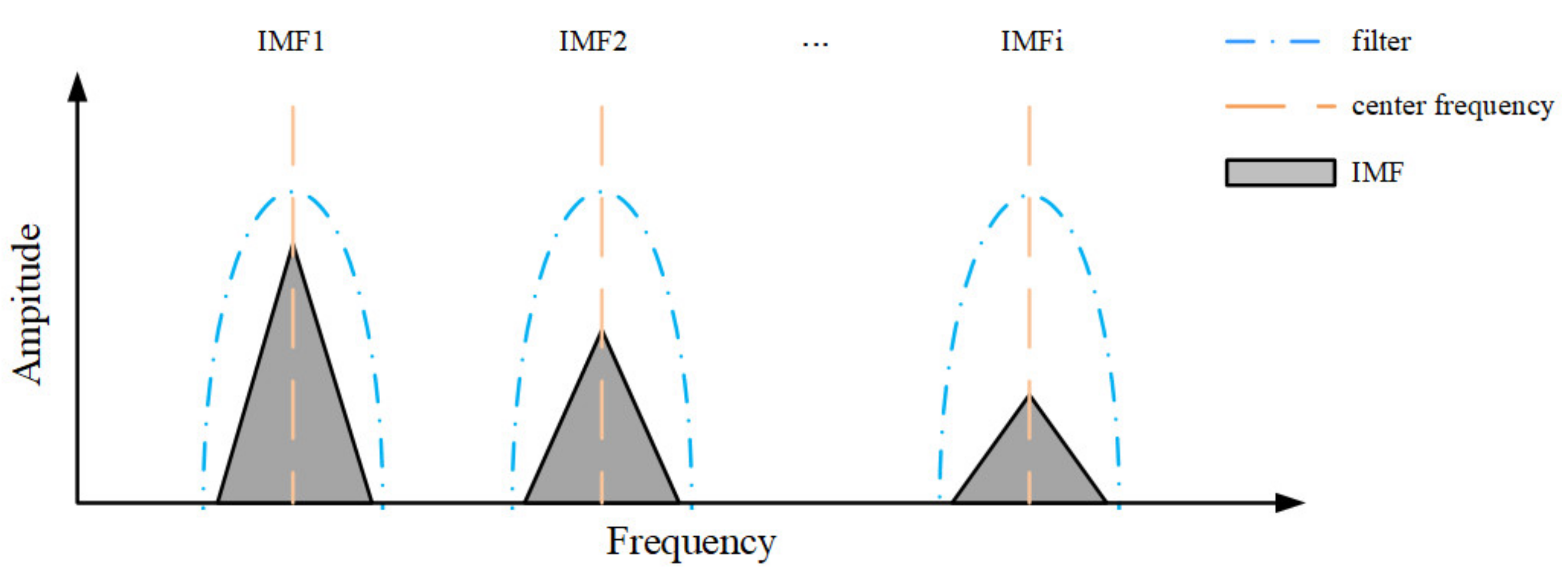
The VMD method is utilized to decompose complex signals into basic functions with diverse forms and different frequency ranges. Its primary purpose is to extract low-frequency and high-frequency modes for signal analysis and processing. The VMD method decomposes the signals into multiple Intrinsic Mode Functions (IMFs) and a residual component, where each IMF corresponds to a vibrating mode within a specific frequency range [43]. The IMFs are obtained by solving a variational problem, showcasing strict bandwidth constraints, and gradually reducing residues. The VMD method allows for bandwidth adjustments as needed and finds wide applications in signal processing, image processing, and data dimensionality reduction fields. The schematic diagram of the VMD method is shown in Figure 2.
The method entails assuming a multi-component signal composed of i finite bandwidth modal components v i t , with each IMF having a center frequency of ω i t . The constrained variational expression ensures that the IMF components have a finite bandwidth with the sum of the center frequencies and estimated bandwidths minimized, while also ensuring that the sum of all modes is equal to the input signal. The constrained variational expression is as follows:
m i n v i , ω i i t δ t + j π t v i t e j ω i t s . t .           i v i t = x t                                            
where v k = v 1 , , v k represents the decomposed IMF components, ω k = ω 1 , , ω k represents the central frequencies of the respective components, t ( ) is the Tikhonov regular term function, δ t is the Dirac function, j denotes the imaginary number, ∗ denotes the convolutional operator, x t is the input signal, δ t + j π t v i t denotes the Hilbert transform, and e j ω i t ) is the frequency modulation operator.
To find the optimal solution, we first introduce the Lagrange multiplier τ t and a second-order penalty factor α , which transforms the constrained variational problem into an unconstrained variational problem. The second-order penalty factor α ensures the accuracy of signal reconstruction in a Gaussian noise environment. The Lagrange multiplier τ t ensures the strictness of the constraint. The extended Lagrange expression is as follows:
L v i , ω i , τ = α i ϑ t δ t + j π t v i t e j ω i t 2 + x t i v i t 2 + τ t , s t k v i t
Then, the Alternating Direction Method of Multipliers (ADMM) is utilized to update each component and its central frequency. The optimal solution to the original problem is ultimately obtained at the saddle point of the unconstrained model. All components can be obtained in the frequency domain as follows:
v ^ k n + 1 ω = s ^ ω i k v ^ i ω + τ ^ ω 2 1 + 2 α ω ω k 2
where ω represents frequency, and v ^ k n + 1 ω , s ^ ω , and τ ^ ω   correspond to the Fourier transforms of v k n ω , s ω , and τ ω .
The VMD method is based on the time-frequency localization characteristics of signals. It decomposes the input signal into multiple modal functions through an iterative optimization process, describing the frequency modulation characteristics of each modal function through frequency modulation parameters. The VMD method can adaptively decompose signals into modal functions with different scales and frequency ranges, making it suitable for various types of signals. Besides, the VMD method provides high decomposition precision, allowing the resulting modal functions to better reflect the local characteristics of the signal.

2.2. CNN

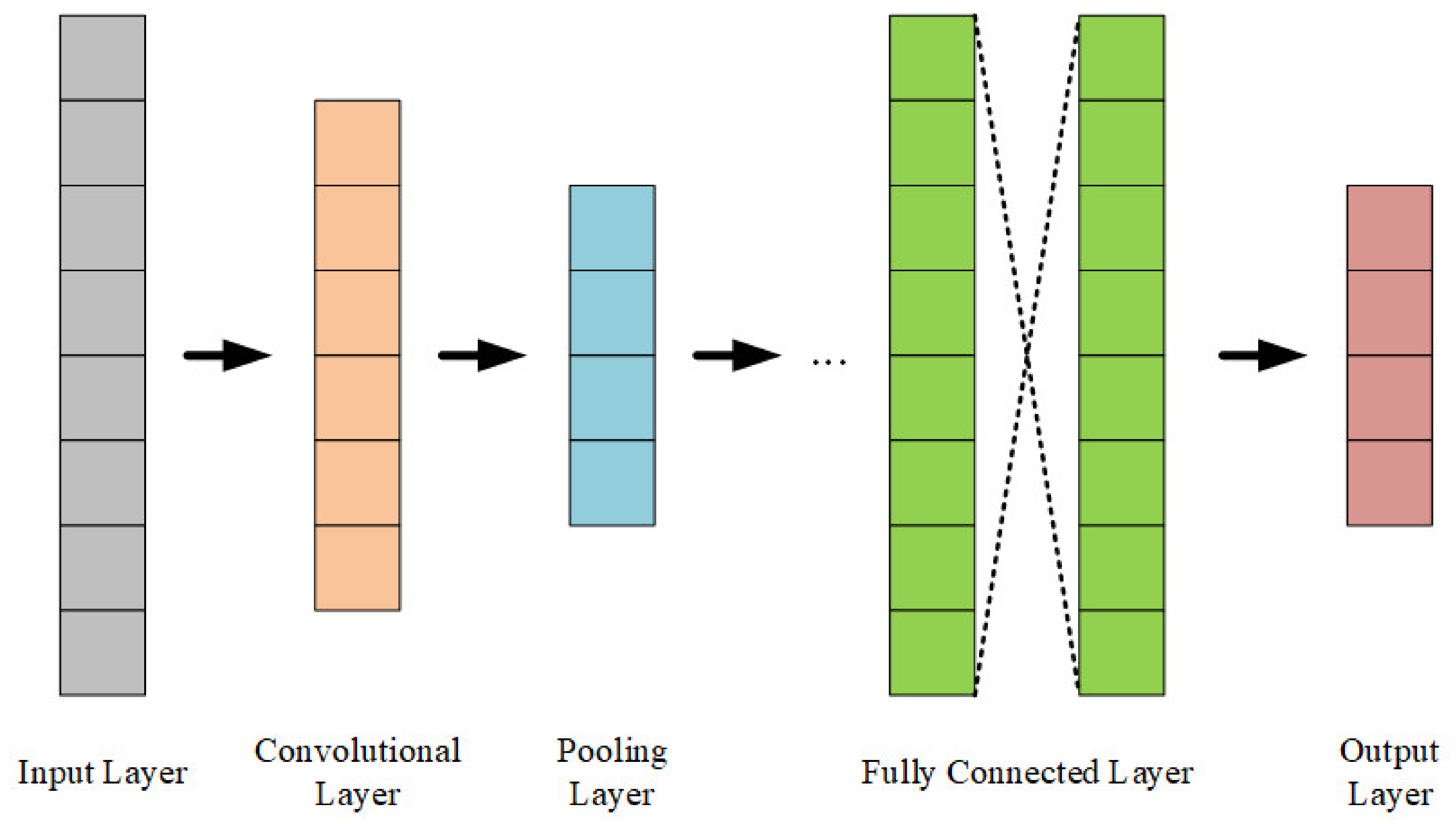
The CNN method is a type of artificial neural network, designed specifically for processing data with grid-like structures. Through convolution operations, the CNN method can effectively identify patterns and features in input data. Composed of multiple convolutional and pooling layers, the CNN method progressively extracts features from input data and ultimately performs classification or prediction. The schematic diagram illustrating its principle is shown in Figure 3:
Figure 3 shows that the convolutional layer, pooling layer, and fully connected layer are the key steps of the CNN method. In this study, the convolution kernel W is a vector. The forward propagation process can be succinctly described as follows:
a 2 = σ z 2 = σ a 1 W 2 + b 2
where a is the input or output dataset, the superscript represents the number of layers in the network,   represents convolution, b represents the bias vector, and σ   is an activation function, usually the rectified linear unit or simply R e L U .
The convolutional layer is the core layer of the CNN method, primarily responsible for convolving input data to extract features. The convolution operation, resembling a sliding window, moves a window across the input data, computing the dot product between the elements within the window and the convolutional kernel to generate a new feature sequence. The convolution operation dimension transformation formula is as follows:
O d = I d k s i z e + 1 s p a d d i n g = V a l i d I d s p a d d i n g = S a m e
where I d   is the input dimension, O d is the output dimension, k s i z e is the size of the convolutional kernel, and s is the stride. In most cases, stacking smaller convolutional kernels is more effective than directly using a single larger convolutional kernel.
The pooling layer is another crucial component in the CNN method, responsible for downsampling input features to reduce the parameter count and prevent overfitting. The formula is as follows:
a ^ l = p o o l a ^ l 1
where p o o l   is the function of reducing the input tensor according to the pooling region and the pooling criteria. The proposed method sets the average pooling, where the average value within each small window is selected as the output, resulting in new pooled features.
The fully connected layer is the final layer in the CNN method, responsible for classifying the features of the pooling layer and mapping them to probabilities of different classes. Its formula is as follows:
a l = σ z l = σ W l a l 1 + b l
where l is the number of layers. Nodes in the fully connected layer form a network where the activation values are transformed into class probabilities using the Softmax function to predict the highest probability class. Each node is connected to the input feature vector, and the activation values are computed using weight matrices and bias vectors, followed by calculating class probabilities through the S o f t m a x function.
The output layer is as follows:
a L = s o f t m a x z L = s o f t m a x W L a L 1 + b L
where L is the number of output layers. The CNN method learns and extracts features through convolutional layers, pooling layers, and fully connected layers for classification or regression tasks. The convolutional layers filter the input GNSS time series through convolution operations to extract local features. The pooling layers downsample the feature dataset to reduce spatial size while retaining essential features. The fully connected layers map the features to the final output.
The CNN method effectively captures local features in GNSS time series through convolution operations and weight sharing, demonstrating strong local perception capabilities. The parameter-sharing mechanism in the CNN method reduces the parameter counts, enhancing training speed and generalization capability. The CNN method has a certain level of invariance through convolution and pooling operations.

2.3. LSTM

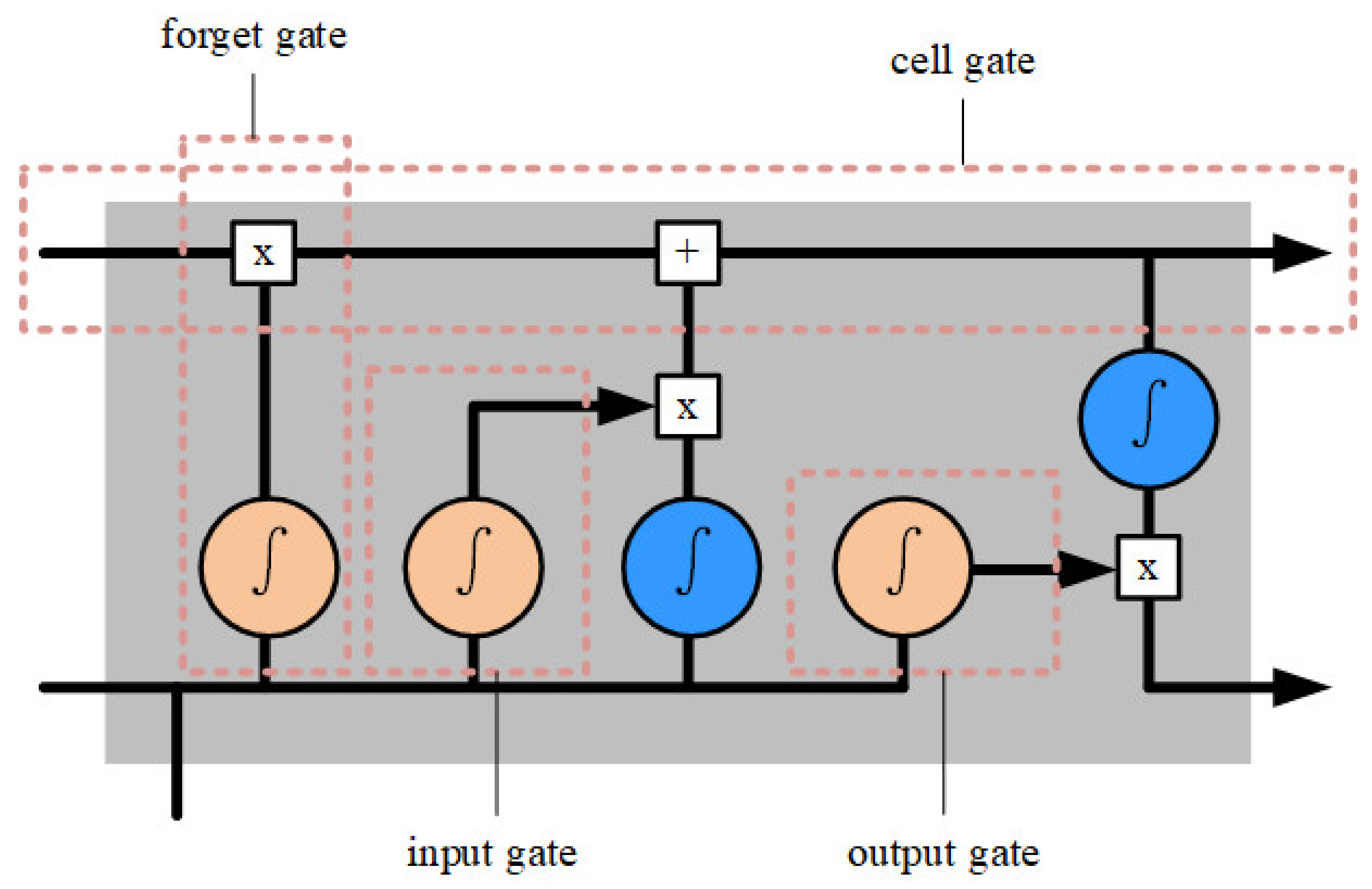
The Recurrent Neural Network (RNN) is a neural network designed for time series, characterized by its recurrent structure, which allows for the propagation and memory of previous states. However, the RNN method suffers from decay over long time intervals, leading to diminished effectiveness in capturing long-term dependencies. To address this challenge, the Long Short-Term Memory (LSTM) network, a specialized RNN method, has been developed. LSTM’s unique design enables it to effectively circumvent long-term dependency issues by inherently retaining early-stage information without incurring significant additional costs. The schematic diagram of the LSTM method is shown in Figure 4.
As shown in Figure 4, there are four key components, including input gate, forget gate, cell gate, and output gate.
The forget gate functions to determine the retention or misplacement in the memory cell from the previous step. This gate uses a sigmoid activation function to determine how to update the cell state, enabling the network to selectively forget unnecessary information. Specifically, the forget gate takes both previous cell state and current input into consideration, outputting a value between 0 and 1 to indicate the ratio of each cell state. The corresponding information is forgotten when the forget gate output is close to 0. Otherwise, the information is retained. The formula of the forget gate is as follows:
f t = σ W f h t 1 , x t + b f
where W f is the weight matrix, b f is the bias term, h t 1 is the hidden state of the previous step, x t is the current input, and σ ( ) is the sigmoid function. This mechanism allows the LSTM method to effectively manage long-term dependencies and better handle GNSS time series.
The input gate functions to control the impact of new input on the cell state. It utilizes a sigmoid activation function to determine what can pass through and be updated into the cell state. Specifically, the input gate performs a weighted sum of the new input and the previous step’s hidden state to determine what needs to be stored or discarded. The formula of the input gate is as follows:
C ˜ t = t a n h W C h t 1 , x t + b C i t = σ W i h t 1 , x t + b i                    
where C ˜ t is the candidate, i t is the value of the input gate, W C , W i is the weight matrix, b C , b i is the bias term, h t 1 is the hidden state of the previous step, x t is the current input, σ ( ) is the sigmoid function, and t a n h ( ) is the hyperbolic tangent function. This mechanism enables the LSTM method to selectively remember or forget certain information, thereby more effectively handling temporal dependencies in long GNSS time series.
The cell gate functions to control the influence of the cell gate by the current input, which filters and integrates input into the cell gate. Specifically, the cell gate uses sigmoid and t a n h functions to generate a candidate for the cell gate. It considers the previous cell gate and the current input and uses multiplication operations to determine what to retain and discard. The formula of the cell gate is as follows:
C t = f t C t 1 + i t C ˜ t
where f t is the output of the forget gate, C t 1 is the previous status of the cell gate, i t is the input gate, and C ˜ t is the candidate. This mechanism allows the LSTM method to effectively control the update of cell gates, capturing important patterns and correlations in sequential data more effectively.
The output gate functions to control the influence of the final output by the current cell gate. It selects the cell gate using s i g m o i d and t a n h functions to generate an output value for the current step. The output gate considers the current cell gate and input gate at the current step, deciding which will be passed to the next layer. The formula of the output gate is as follows:
o t = σ W o h t 1 , x t + b o ) h t = o t tan h C t                    
where W o is the weight matrix, b o is the bias term, h t 1 is the hidden state of the previous step, x t is the current input, σ ( ) is the sigmoid function, and t a n h ( ) is the hyperbolic tangent function. This mechanism allows the LSTM network to effectively produce appropriate outputs based on the current cell gate and input gate, enhancing its ability to handle and predict GNSS time series.
The LSTM method is effective in handling long-term dependencies in GNSS time series, making it suitable for capturing long-span dependencies. These mechanisms help alleviate the vanishing and exploding gradient problems, making the model easier to train. Additionally, the memory cells can retain and update information over periods, aiding in capturing long-term dependencies in GNSS time series.

3. Experiment

Tow experiments are given in this section. The first experiment is performed to prove the feasibility of the proposed method, and the second experiment is performed to give a comparison for the proposed method with the extended Kalman filter (EKF).

3.1. The Feasibility Experiment

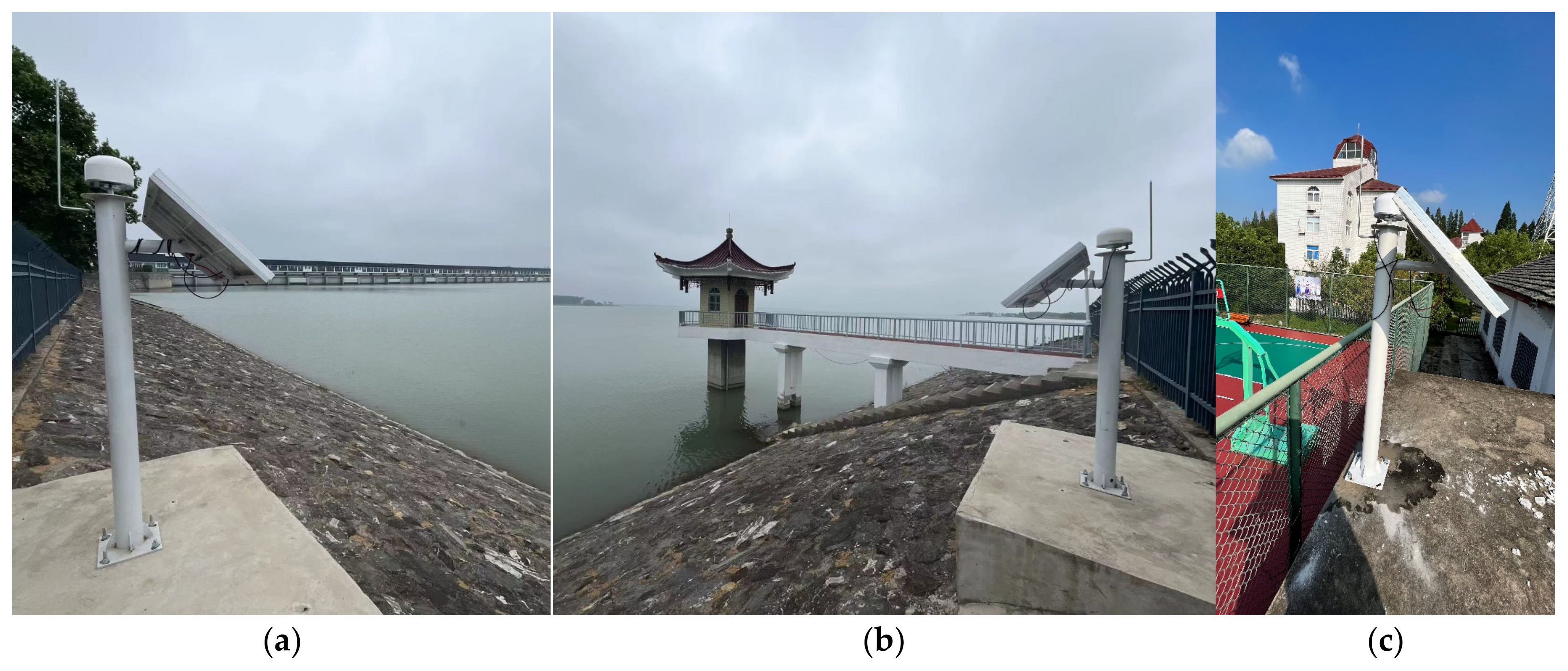
The experiment was conducted at the Sanhe sluice of Hongze Lake, Jiangsu, China, whose configuration parameters are shown in Table 1. The monitoring site and the reference site are shown in Figure 5.
This study validates the effectiveness of the proposed method using east (E)-direction time series as an example. We use 80% of the time series as the training set and the remaining 20% as the validation set. A 24 h extrapolation is provided at the end for prediction. First, the results of the CNN–LSTM method are shown in Figure 5. In the following experiment, we choose the mean-square error (MSE) as the instantaneous function because it can better reflect the gradient changes during the training of neural networks for regression problems.
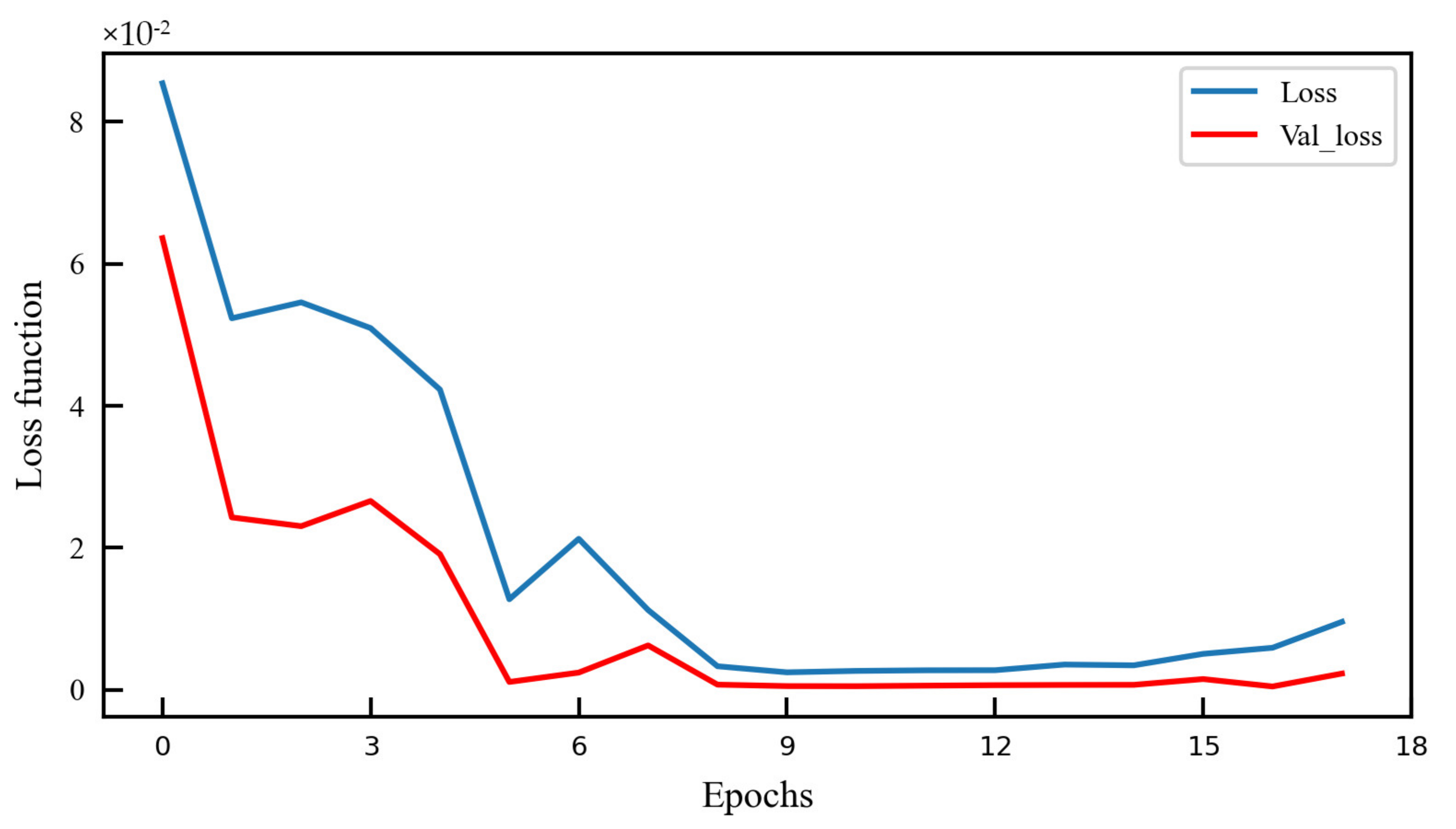
Figure 6 illustrates the curve of the loss function of the training process, in which the number of iterations is set to 17. Legend loss, also known as training loss, quantifies the disparity between the model’s predictions and the actual observations during the training phase. Conversely, val_loss, or validation loss, highlights the deviation between the model’s predictions and the validation data, serving as an indicator of the model’s performance on unseen data. As the number of training iterations increases, the loss function gradually decreases, indicating that the model is converging. In the initial phase (1st–8th epoch), the loss function decreases rapidly, then levels off from the 8th to 17th epoch, eventually converging to a low value. This suggests that after eight epochs of training, the loss function has stabilized, and further increasing the number of training iterations has little impact on performance improvement.
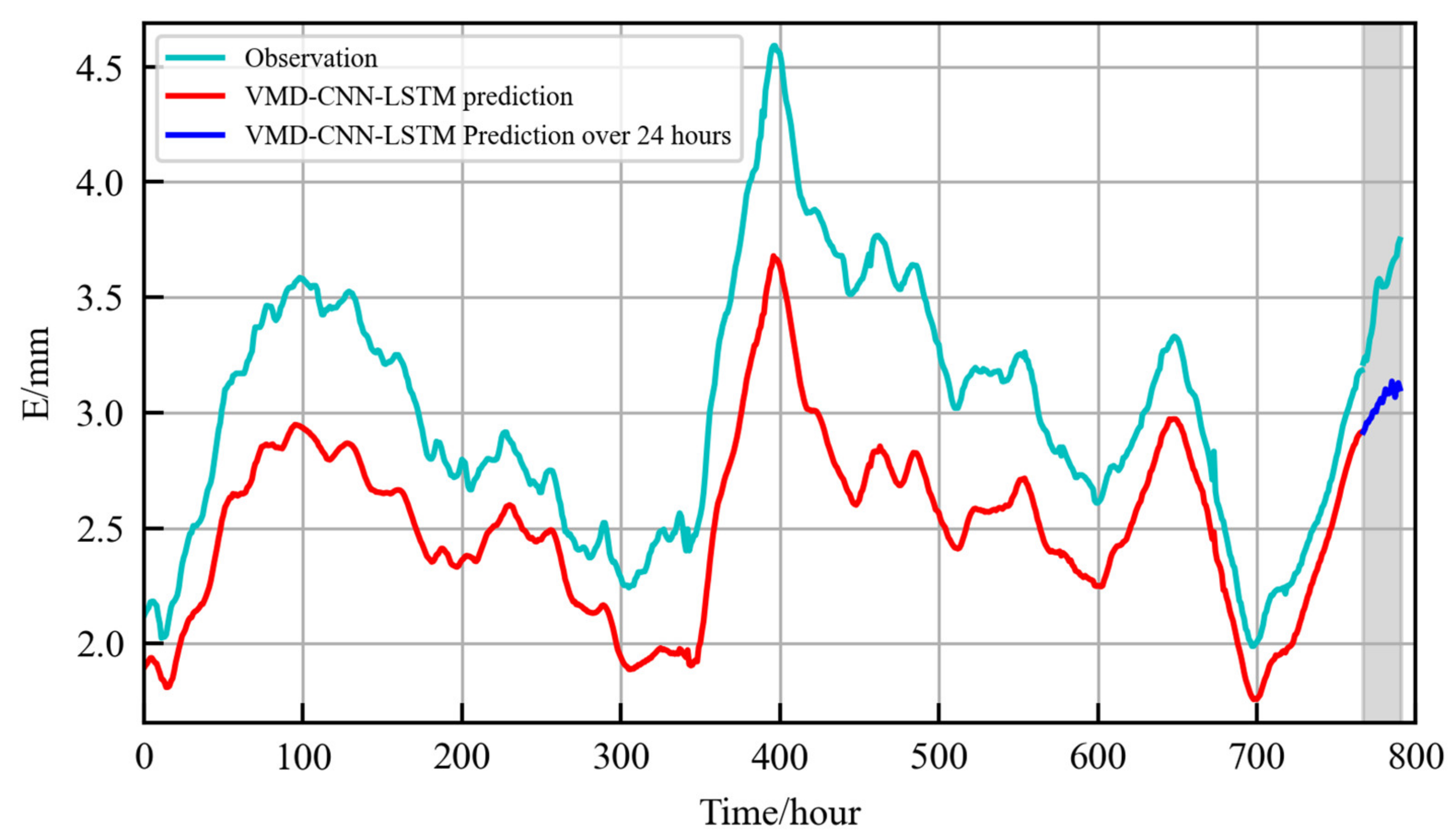
Figure 7 illustrates the observation, model prediction, and extrapolated forecast for the next 24 h in the GNSS time series. The overall trend of the observation aligns with the model prediction, but their agreement is moderate with a maximum difference of approximately 2 mm. Particularly, in the range of the 600th to 800th hour, the consistency between the two is poorer, indicating that the neural network captures features poorly within this interval. Additionally, the 24 h extrapolated forecast in the figure demonstrates the model’s ability to predict, showing a trend of increase followed by a decrease, providing us with some insights into the changing trends within the next day. Figure 7 shows that it is necessary to take additional measures to obtain a better prediction. Firstly, decomposition and analysis of the original GNSS time series are provided.
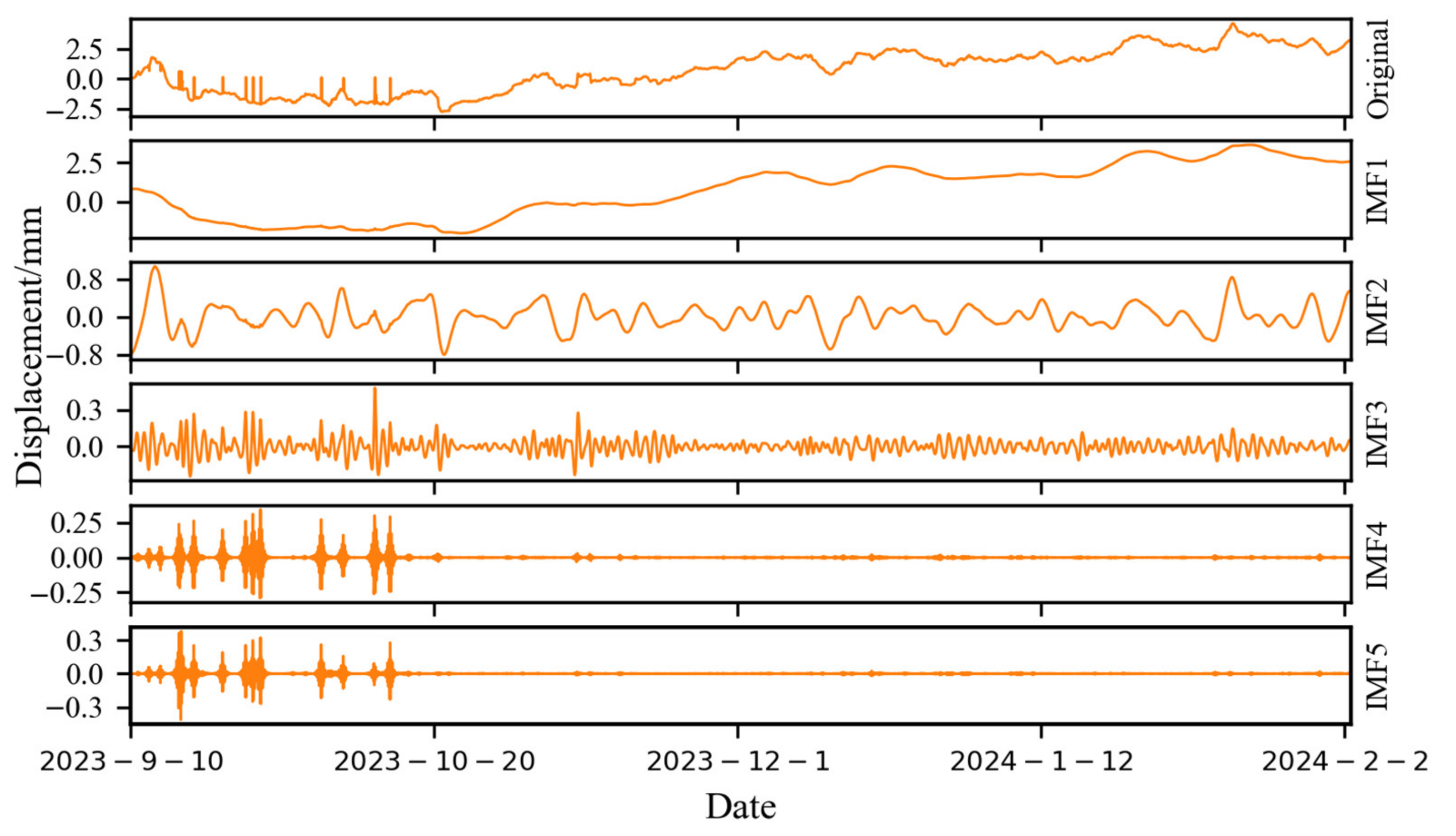
Figure 8 depicts the original GNSS time series and the IMFs of the VMD method. The original signal exhibits abrupt changes between 10 September 2023 and 20 October 2023, while showing jagged fluctuations for the remaining period. The VMD method decomposes the original signal into several modal components with different frequencies and amplitudes. Each modal component can be referred to as an IMF and represents a local pattern or oscillation mode in the original signal, with a better show of the local features and periodic variations in the original signal. IMF1 is the lowest-frequency component, typically encompassing the slowest-changing patterns, which represents the long-term effects. IMF2 shows low-frequency fluctuations, with a maximum fluctuation range of approximately 0.8 mm. It represents foundation settlement. IMF3 represents the medium-frequency fluctuations, exhibiting noticeable fluctuations during the abrupt changes and jagged fluctuations of the original signal, with a maximum fluctuation of about 0.3 mm. It represents deformations caused by cyclical loads. IMF4 represents the high-frequency fluctuations, which represents deformations caused by resonance. IMF5 depicts the high-frequency vibration patterns, reflecting the potential noise interference, with a maximum fluctuation of about 0.3 mm corresponding to the abrupt changes in the original signal. The VMD method also aids in extracting important information and periodic variations in the original signal, facilitating signal processing, feature extraction, and other applications. Through the analysis of the IMFs shown in the figure, we can delve deeper into the underlying structure and features of the GNSS time series, providing valuable references and foundations for subsequent analysis and applications. Figure 8 shows that IMFs have different characteristics, and it is better to apply different parameters for different IMFs in the CNN–LSTM method.
Figure 9 illustrates the curve of the loss function of the training process of IMF1, in which the number of iterations is set to 40. As the number of training iterations increases, the loss function gradually decreases, indicating that the model is converging. In the initial phase (1st–12th epoch), the loss function decreases rapidly, then levels off from the 12th to 17th epoch, eventually converging to a low value. This suggests that after 12 epochs of training, the loss function of IMF1 has stabilized.
Figure 10 illustrates the observation, model prediction, and extrapolated forecast for the next 24 h of IMF1. The overall trend of the observation aligns with the prediction, with a maximum difference of approximately 0.6 mm. In contrast with Figure 7, IMF1 has a smaller difference and better consistency. Particularly, in the range of the 700th to 800th hour, the consistency between the two is better, while the original is poor. Additionally, the 24 h extrapolated forecast in Figure 10 demonstrates a better prediction than that in Figure 7.
To enhance prediction reliability, the subsequent 24 h of data are excluded from the test set. However, decomposing only the 24 h data would result in a time series that is too short, making it challenging to detect the correct signal components and disrupting continuity between the test set and the 24 h outcome. Consequently, the figure cannot depict the IMF observation line for the next 24 h. The reconstructed overall signal, derived from the processed prediction of the IMFs, is compared with the original time series to assess the performance of the proposed method.
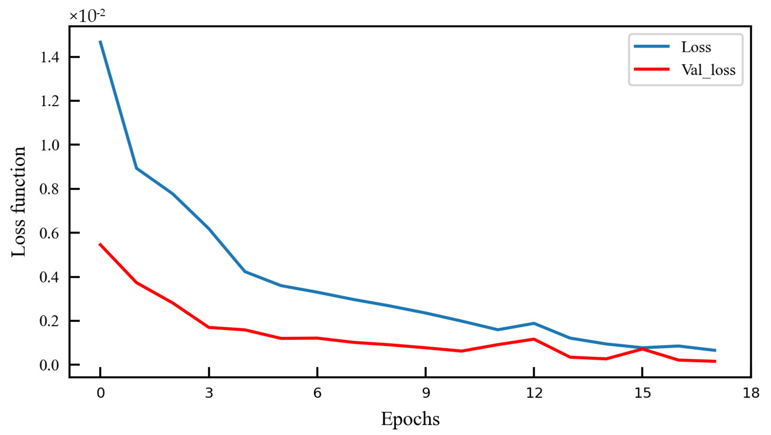
Figure 11 illustrates the curve of the loss function of the training process of IMF2, in which the number of iterations is set to 50. As the number of training iterations increases, the loss function gradually decreases, indicating that the model is converging. In the initial phase (1st–7th epoch), the loss function decreases rapidly, then levels off from the 8th to 30th epoch, and then the loss function decreases slowly. After the 30th epoch, the loss function eventually converges to a low value. In contrast to Figure 7 and Figure 9, Figure 10 has better consistency with no repetition.
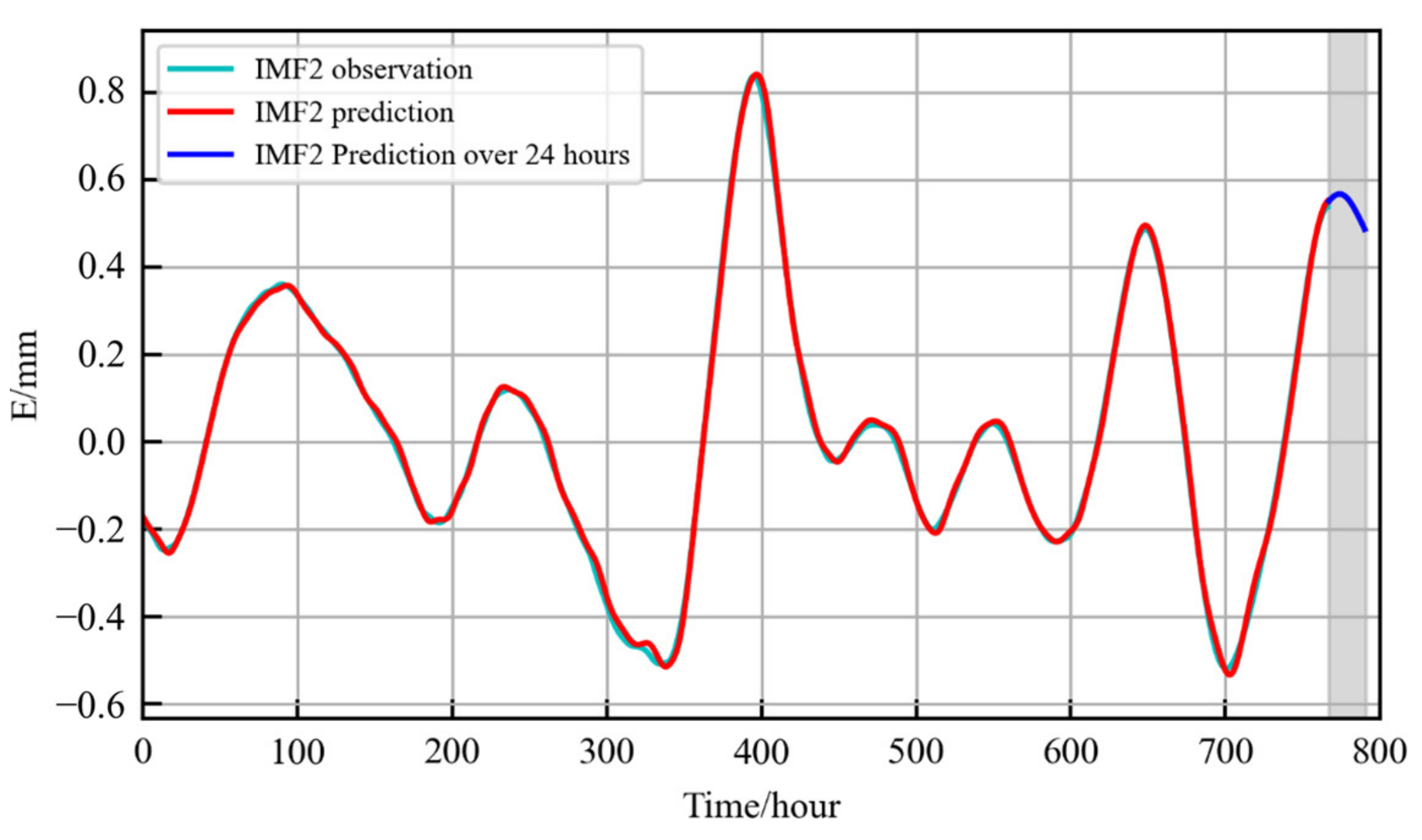
Figure 12 illustrates the observation, model prediction, and extrapolated forecast for the next 24 h of IMF2. The overall trend of the observation aligns with the model prediction perfectly. Additionally, the 24 h extrapolated forecast in the figure demonstrates the model’s ability to predict, showing a trend of increase followed by a decrease, providing us with some insights into the changing trends within the next day. Figure 12 shows a better consistency than Figure 7 and Figure 10.
Figure 13 illustrates the curve of the loss function of IMF3, in which the number of iterations is set to 17. As the number of training iterations increases, the loss function gradually decreases, indicating that the model is converging. In the initial phase (1st–9th epoch), the loss function decreases rapidly, then levels off from the 10th to 17th epoch, eventually converging to a low value. This suggests that after a certain amount of training, the loss function has stabilized, which is similar to the situation in Figure 6 and Figure 9.
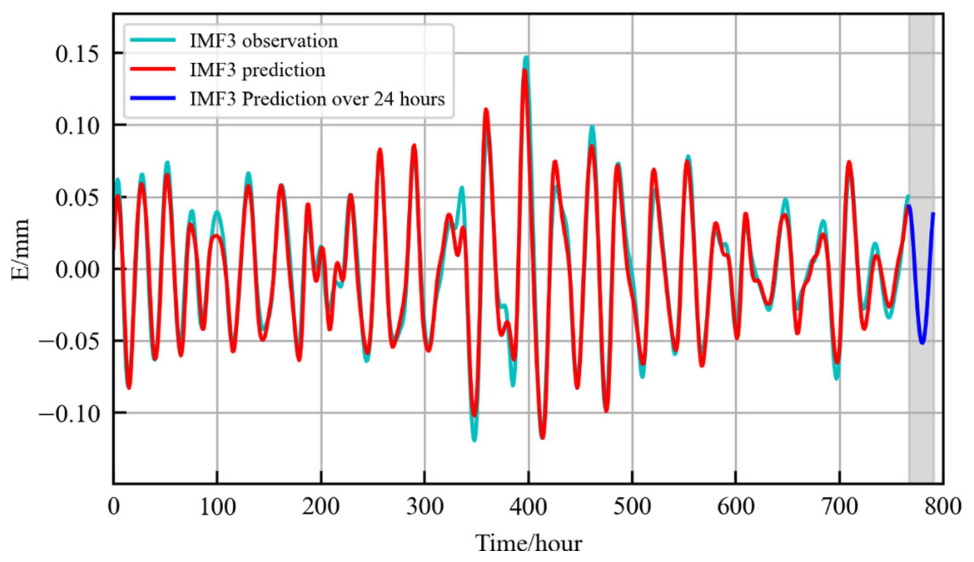
Figure 14 illustrates the observation, model prediction, and extrapolated forecast for the next 24 h of IMF3. The overall trend of the observation perfectly aligns with the model prediction for most of the period, but there are some slight differences, such as from the 300th–400th hour. Additionally, the 24 h extrapolated forecast in the figure demonstrates the model’s ability to predict, showing a trend of increase followed by a decrease.
Figure 15 illustrates the curve of the loss function of IMF4, in which the number of iterations is set to 50. As the number of training iterations increases, the loss function gradually decreases, indicating that the model is converging. In the initial phase (1st–20th epoch), the loss function decreases rapidly, then levels off from the 21st to 50th epoch, eventually converging to a low value with a slight difference. This suggests that after a certain amount of training, the loss function has stabilized, and further increasing the number of training iterations has little impact on performance improvement.
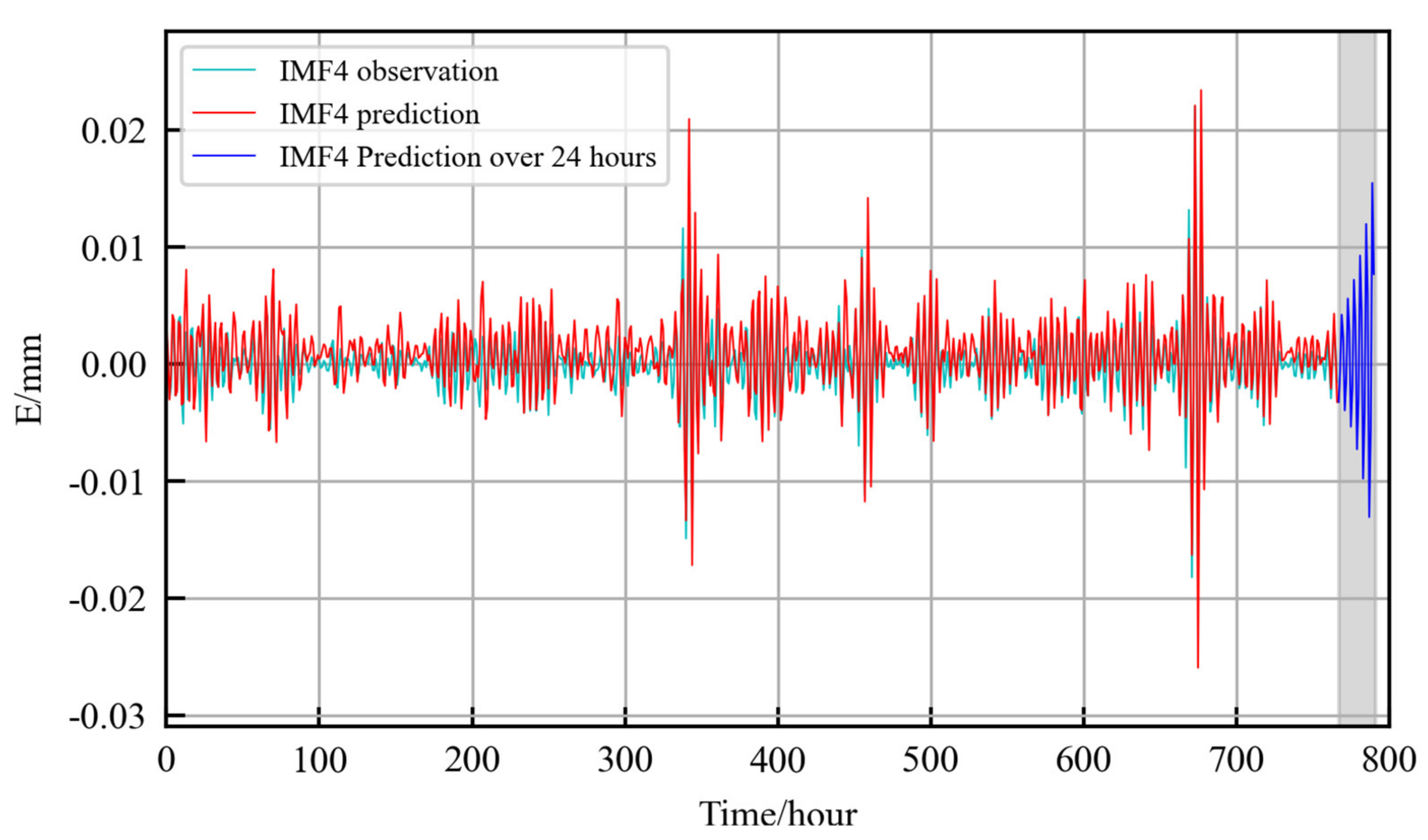
Figure 16 illustrates the observation, model prediction, and extrapolated forecast for the next 24 h of IMF4. The overall trend of the observation aligns with the model prediction perfectly, but there are two significantly different periods in which the prediction has a 0.01 mm difference with the observation, such as periods around the 350th hour and 770th hour. Additionally, the 24 h extrapolated forecast in the figure demonstrates the model’s ability to predict, showing a maximum range of about 0.04 mm. Figure 16 shows an abnormal range of the 24 h extrapolated forecast.
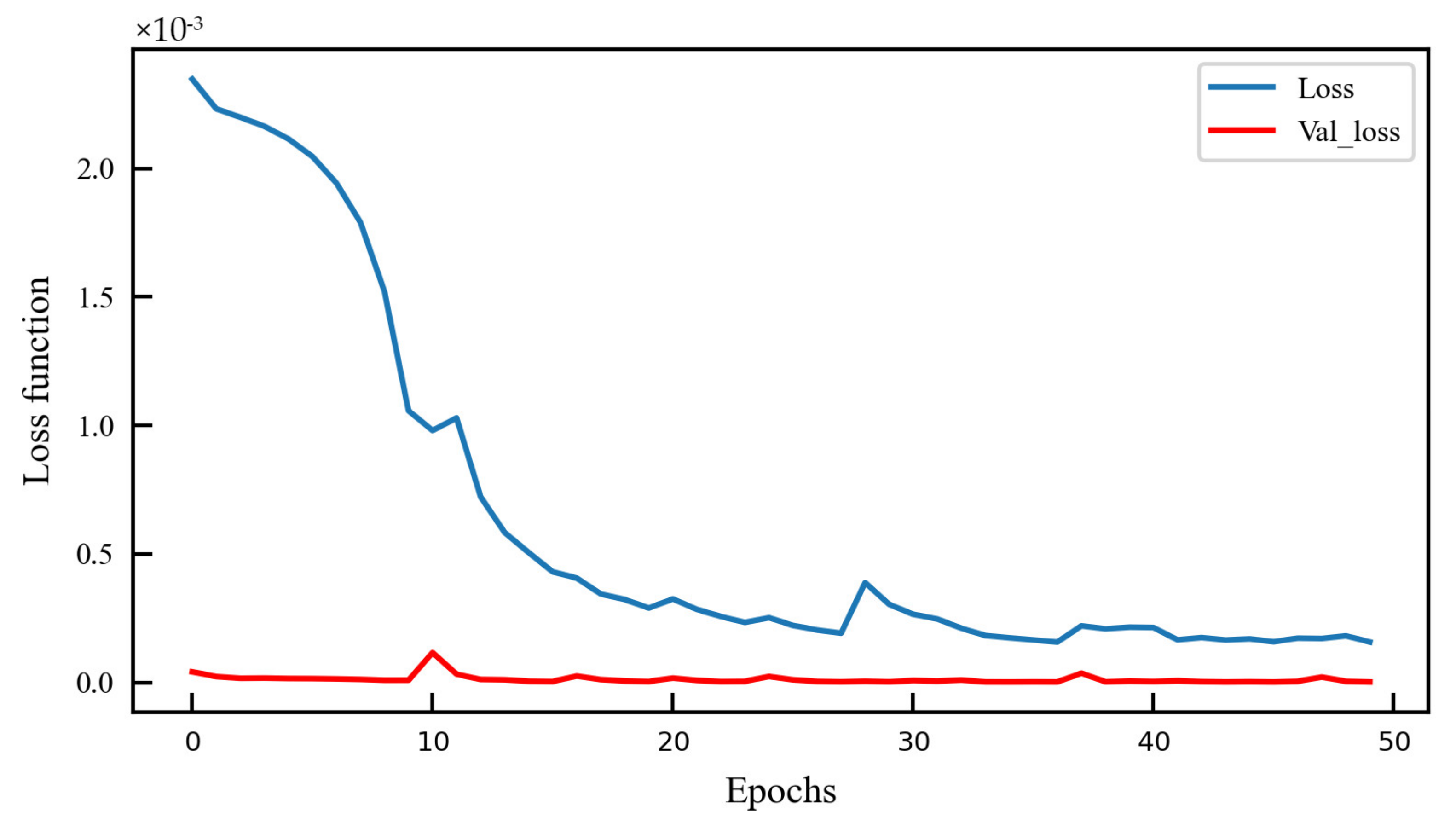
Figure 17 illustrates the curve of the loss function of IMF5, in which the number of iterations is set to 50. As the number of training iterations increases, the loss function gradually decreases, indicating that the model is converging. In the initial phase (1st–30th epoch), the loss function decreases rapidly, then levels off from the 31st to 50th epoch, eventually converging to a low value with a slight difference. This suggests that after a certain amount of training, the loss function has stabilized, and further increasing the number of training iterations has little impact on performance improvement.
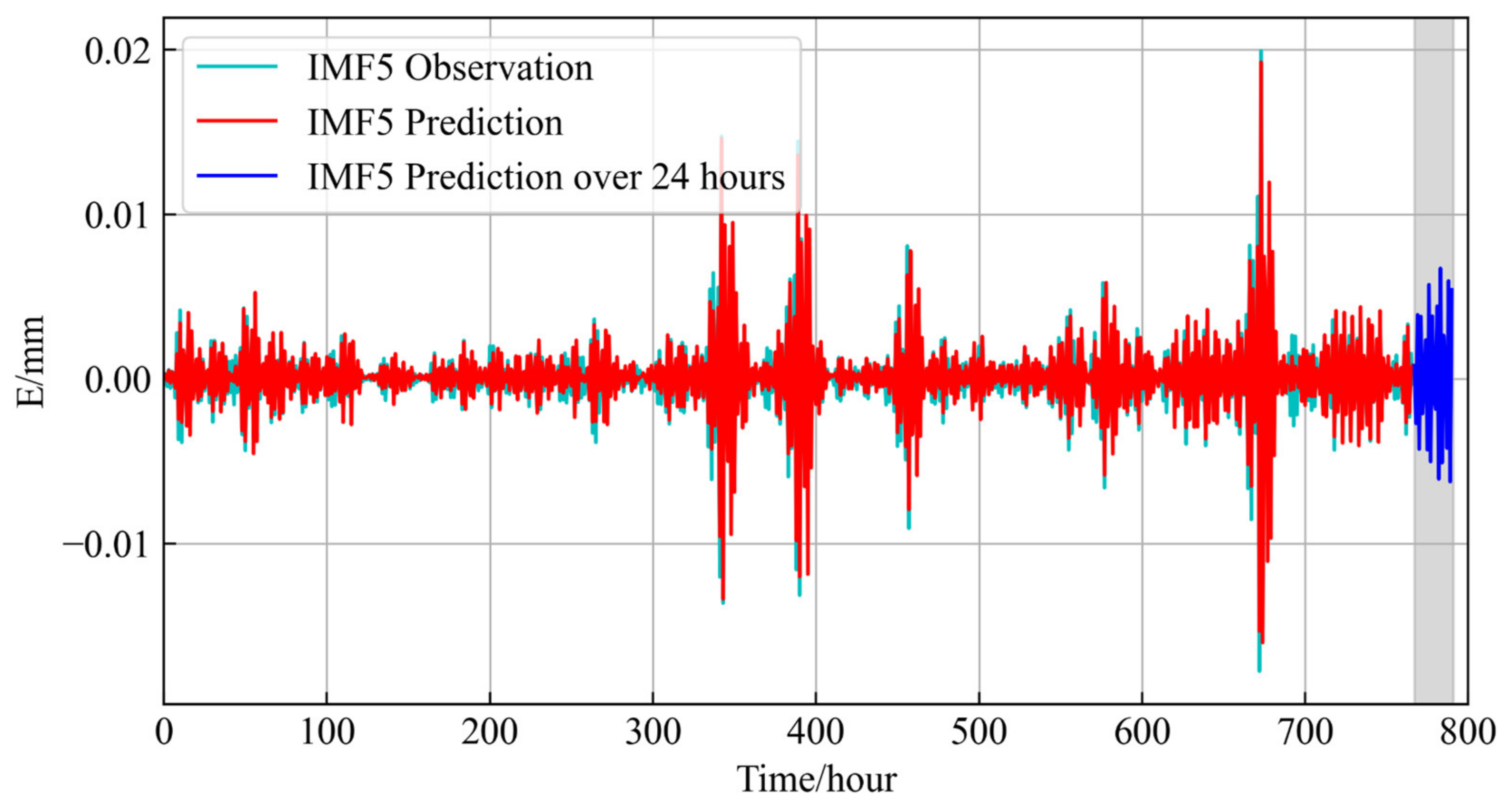
Figure 18 illustrates the observation, model prediction, and extrapolated forecast for the next 24 h of IMF5. The overall trend of the observation aligns with the model prediction, but their agreement is moderate with a maximum difference of approximately 0.01 mm. Additionally, the 24 h extrapolated forecast in the figure demonstrates the model’s ability to predict, showing a trend of increase followed by a decrease, providing us with some insights into the changing trends within the next day.
Figure 19 illustrates the observation, model prediction, and extrapolated forecast for the next 24 h of the VMD-CNN-LSTM method. In contrast with Figure 7, Figure 19 has better consistency with a maximum of about 0.6 mm. Particularly, in the range of the 600th to 800th hour, the prediction of the VMD-CNN-LSTM method has a perfect consistency. Additionally, the 24 h extrapolated forecast shows a trend of increase followed by a decrease, which is better than the CNN–LSTM method. In general, the original GNSS time series has different IMFs with different characteristics. It is better to apply different parameters to obtain better predictions.
The evaluation metrics for the prediction performance of IMFs, including the root mean square error (RMSE), mean-square error (MSE), mean absolute error (MAE), and R-squared (R2), are presented in Table 2. These metrics are utilized to assess the prediction accuracy for each IMF component, revealing the performance differences across different frequency components. It can be observed that the RMSE, MSE, and MAE metrics reflect the prediction accuracy of the model, with only slight discrepancies in the accuracy of IMF1 compared to the others. Furthermore, R², as a measure of the model’s goodness of fit, indicates that IMF2 and IMF3 exhibit good fitting, while IMF1, IMF4, and IMF5 show slightly lower fitting performance.
For further comparison, Figure 20 compares the error statistics of the CNN–LSTM method and the VMD-CNN-LSTM method. The left panel displays the error distribution and curve fitting of the CNN–LSTM method, with errors mainly concentrated in the (−3, 1) range and a central value of approximately −0.8 mm for the fitted curve. The right panel illustrates the error distribution and curve fitting of the VMD-CNN-LSTM method, with errors primarily distributed in the (−2.5, 1.8) range and a central value of about −0.2 mm for the fitted curve. Besides, the proposed method has an improvement of about 75% compared with the CNN–LSTM method. In general, the proposed method, by applying different parameters to different IMFs, achieves better prediction performance.

3.2. The Comparative Experiment

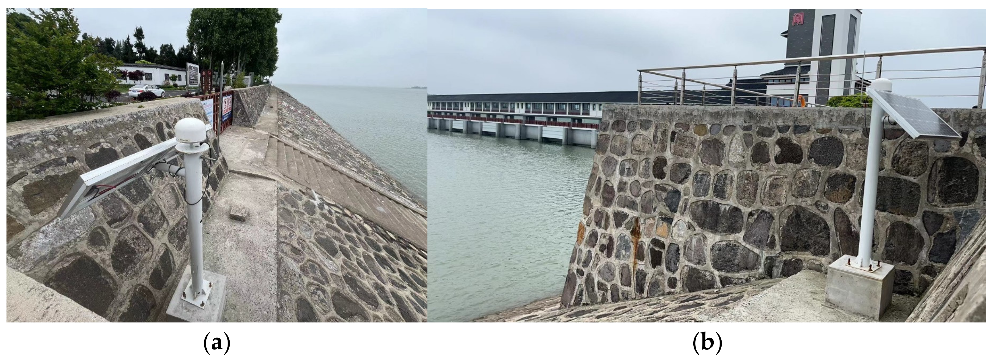
The above experiment proves the feasibility of the proposed VMD-CNN-LSTM method, and the experiment in this section is performed to give a comparison between the proposed method and the EKF. The experiment was also conducted at the Sanhe sluice of Hongze Lake but at a different monitoring station. Figure 21 demonstrates the surrounding environment of this new monitoring station The experimental period is from 10 September 2023–24 April 2024, and other configuration parameters are the same as the above experiment.
Table 3 presents performance metrics for the EKF and the VMD-CNN-LSTM method. The overall assessment reveals significant enhancements across all metrics with the proposed VMD-CNN-LSTM method relative to the EKF, indicating superior accuracy and reliability in GNSS deformation monitoring for hydraulic structures. Specifically, compared to the EKF, the employment of VMD-CNN-LSTM results in approximately a 67.16% reduction in the MSE, a 42.62% decrease in the RMSE, a 43.28% decrease in the MAE, and a 6.88% increase in R2. In summary, the VMD-CNN-LSTM method demonstrates clear advantages in geophysical process analysis, offering more precise and dependable outcomes for geological structure analysis.
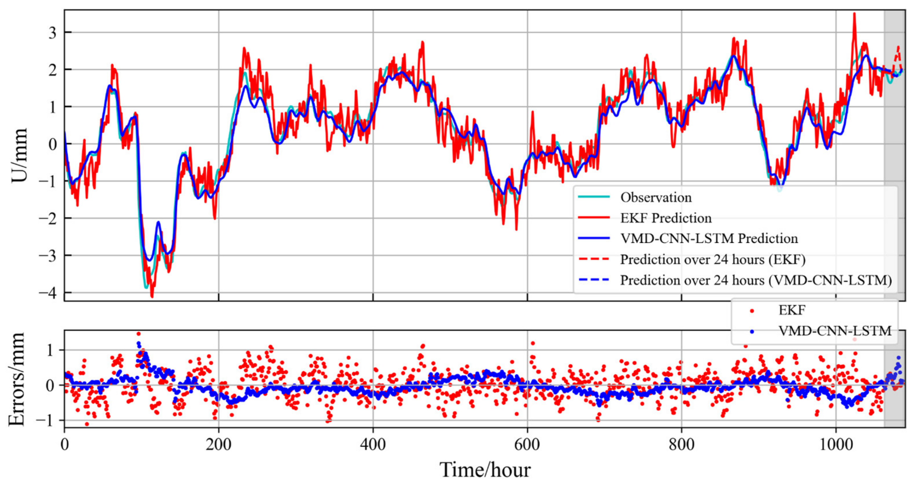
Figure 22 presents a comparison between the proposed VMD-CNN-LSTM and EKF methods, focusing on both the test dataset and 24 h extrapolation results. The figure comprises a time series plot and an error scatter plot. In the time series plot, the VMD-CNN-LSTM method shows a closer alignment with the original observations from the test dataset, while the EKF method demonstrates more frequent fluctuations throughout the process. The error scatter plot corroborates the findings from the time series plot, indicating that the results obtained with VMD-CNN-LSTM are markedly better than those from the EKF. Around the 120th hour, the EKF exhibits prediction errors of approximately 1 mm, while VMD-CNN-LSTM remains more consistent with fewer and less pronounced deviations over the entire interval. Overall, the VMD-CNN-LSTM method outperforms the EKF, delivering more accurate and stable predictions.

4. Discussion

The VMD method is a global optimization method aimed at decomposing the GNSS time series into various modes with distinct frequencies and amplitudes. By minimizing the distances between the signal and each mode, it effectively extracts periodic components and vibration characteristics. However, overlapping frequencies between modes may lead to unclear decomposition outcomes, and noise in the signal also impacts the efficacy of the VMD method. In the future, we will try to apply spectral decomposition methods to separate overlapping vibration modes.
The CNN method can extract features that effectively identify features in GNSS time series, reducing the risk of overfitting, and improving the generalization ability. However, the CNN method has poorer performance for time series than the RNN method. Therefore, an LSTM method is adopted in the subsequent process.
LSTM is one of the RNN methods, which can capture long-term dependencies in GNSS time series. It effectively addresses the gradient problem and aids in prediction for long-time series. Besides, it can also be applied to GNSS time series of different lengths. However, its complex algorithm increases the computational cost of training and inference. To address these issues, we will apply attention mechanisms to enhance the performance and efficiency of LSTM models in the future.
However, several factors can impact the performance of VMD-CNN-LSTM in GNSS deformation monitoring. Firstly, poor data quality, characterized by significant noise contamination or a high proportion of missing values, can hinder the accurate extraction of useful information for prediction. Secondly, for excessively long time series spanning years or more, the model may struggle to effectively capture long-term trends and patterns. Thirdly, the presence of highly complex nonlinear patterns, arising from interactions among multiple factors, may pose challenges for VMD-CNN-LSTM in modeling and predicting deformation accurately. Besides, limited training data availability can impede the model’s ability to fully learn patterns within the time series, thereby affecting its predictive capacity. Moreover, in specific environments such as extreme weather conditions, seismic activity, or instances of human interference, anomalous behavior in GNSS deformation monitoring may exceed the predictive capabilities of VMD-CNN-LSTM, particularly when confronted with limited data samples. These considerations underscore the importance of carefully assessing the suitability of VMD-CNN-LSTM for deformation monitoring tasks under various conditions, while also highlighting potential avenues for future research to address these challenges.

5. Conclusions

In this study, we have introduced a novel methodology based on VMD, CNN, and LSTM for enhancing the accuracy of time series prediction. By leveraging the strengths of these three components within a unified framework, our proposed VMD-CNN-LSTM method has demonstrated promising results in capturing complex temporal patterns and improving predictive performance. The VMD method decomposes the original GNSS time series into IMFs, enabling the isolation of inherent oscillatory modes and trends. The subsequent CNN method facilitates the extraction of features from the decomposition, allowing the model to discern important patterns at multiple scales. The further LSTM method facilitates the refinement and prediction of time series outcomes with improved accuracy and adaptability to diverse temporal dynamics. The experiment proves that the proposed method has an improvement of about 75% over the CNN–LSTM method. By integrating VMD, CNN, and LSTM in a unified framework, our study aims to contribute to the advancement of time series forecasting techniques and pave the way for enhanced predictive modeling in diverse domains.

Author Contributions

Conceptualization, Y.X., X.M. and H.L.; data curation, H.L. and J.W.; formal analysis, J.D. and X.M.; funding acquisition, J.W. and Y.J.; methodology, H.L., X.L. and Y.Y.; project administration, J.W.; resources, J.W. and Y.J.; software, H.L. and Y.X.; writing—original draft, H.L.; writing—review and editing, X.M. and Y.X. All authors have read and agreed to the published version of the manuscript.

Funding

This research was funded by the Jiangsu Provincial Department of Water Resources, grant numbers 2022050 and 2022083, and the Jiangsu Hydraulic Research Institute, grant number 2023z036 and 2023z045.

Data Availability Statement

The data presented in this study are available on request from the corresponding authors.

Conflicts of Interest

The authors declare no conflicts of interest.

References

  1. Strygina, M.A.; Gritsuk, I.I. Hydrological safety and risk assessment of hydraulic structures. RUDN J. Eng. Res. 2018, 19, 317–324. [Google Scholar] [CrossRef]
  2. Tian, D.; Liu, H.; Chen, S.; Li, M.; Liu, C. Human error analysis for hydraulic engineering: Comprehensive system to reveal accident evolution process with text knowledge. J. Constr. Eng. Manag. 2022, 148, 04022093. [Google Scholar] [CrossRef]
  3. Hudnut, K.W.; Behr, J.A. Continuous GPS Monitoring of Structural Deformation at Pacoima Dam, California. Seismol. Res. Lett. 1998, 69, 299–308. [Google Scholar] [CrossRef]
  4. Rossi, G.; Zuliani, D.; Fabris, P. Long-term GNSS measurements from the northern Adria microplate reveal fault-induced fluid mobilization. Tectonophysics 2016, 690, 142–159. [Google Scholar] [CrossRef]
  5. Dardanelli, G.; Pipitone, C. Hydraulic models and finite elements for monitoring of an earth dam, by using GNSS techniques. Period. Polytech. Civ. Eng. 2017, 61, 421–433. [Google Scholar] [CrossRef]
  6. Barzaghi, R.; Cazzaniga, N.E.; De Gaetani, C.I.; Pinto, L.; Tornatore, V. Estimating and comparing dam deformation using classical and GNSS techniques. Sensors 2018, 18, 756. [Google Scholar] [CrossRef] [PubMed]
  7. Riguzzi, F.; Devoti, R.; Pietrantonio, G. GNSS data provide unexpected insights in hydrogeologic processes. Bull. Geophys. Oceanogr. 2021, 62, 637–646. [Google Scholar] [CrossRef]
  8. Jiang, W.; Liang, Y.; Yu, Z.; Xiao, Y.; Chen, Y.; Chen, Q. Progress and thoughts on application of satellite positioning technology in deformation monitoring of water conservancy projects. Geomat. Inf. Sci. Wuhan Univ. 2022, 47, 1625–1634. [Google Scholar]
  9. Harvey, A.C. Forecasting, Structural Time Series Models and the Kalman Filter; Cambridge University Press: Cambridge, UK, 1990. [Google Scholar]
  10. De Lannoy, G.J.; Reichle, R.H.; Houser, P.R.; Pauwels, V.R.; Verhoest, N.E. Correcting for forecast bias in soil moisture assimilation with the ensemble Kalman filter. Water Resour. Res. 2007, 43, 9. [Google Scholar] [CrossRef]
  11. Cassola, F.; Burlando, M. Wind speed and wind energy forecast through Kalman filtering of Numerical Weather Prediction model output. Appl. Energy 2012, 99, 154–166. [Google Scholar] [CrossRef]
  12. Kalnay, E.; Ota, Y.; Miyoshi, T.; Liu, J. A simpler formulation of forecast sensitivity to observations: Application to ensemble Kalman filters. Tellus A Dyn. Meteorol. Oceanogr. 2012, 64, 18462. [Google Scholar] [CrossRef]
  13. Lu, F.; Zeng, H. Application of Kalman filter model in the landslide deformation forecast. Sci. Rep. 2020, 10, 1028. [Google Scholar] [CrossRef] [PubMed]
  14. Lin, Y.-H.; Lee, P.-C. Novel high-precision grey forecasting model. Autom. Constr. 2007, 16, 771–777. [Google Scholar] [CrossRef]
  15. Ho, P.H. Forecasting construction manpower demand by gray model. J. Constr. Eng. Manag. 2010, 136, 1299–1305. [Google Scholar] [CrossRef]
  16. Chang, C.-J.; Li, D.-C.; Huang, Y.-H.; Chen, C.-C. A novel gray forecasting model based on the box plot for small manufacturing data sets. Appl. Math. Comput. 2015, 265, 400–408. [Google Scholar] [CrossRef]
  17. Yang, F.; Tang, X.; Gan, Y.; Zhang, X.; Li, J.; Han, X. Forecast of freight volume in Xi’an based on gray GM (1, 1) model and Markov forecasting model. J. Math. 2021, 2021, 6686786. [Google Scholar] [CrossRef]
  18. Wang, Z.-X.; He, L.-Y.; Zhao, Y.-F. Forecasting the seasonal natural gas consumption in the US using a gray model with dummy variables. Appl. Soft Comput. 2021, 113, 108002. [Google Scholar] [CrossRef]
  19. Newbold, P. ARIMA model building and the time series analysis approach to forecasting. J. Forecast. 1983, 2, 23–35. [Google Scholar] [CrossRef]
  20. Van Der Voort, M.; Dougherty, M.; Watson, S. Combining Kohonen maps with ARIMA time series models to forecast traffic flow. Transp. Res. Part C Emerg. Technol. 1996, 4, 307–318. [Google Scholar] [CrossRef]
  21. Meyler, A.; Kenny, G.; Quinn, T. Forecasting Irish Inflation Using ARIMA Models. Cent. Bank Financ. Serv. Auth. Irel. Tech. 1998, 3, 1–48. [Google Scholar]
  22. Siami-Namini, S.; Tavakoli, N.; Namin, A.S. A comparison of ARIMA and LSTM in forecasting time series. In Proceedings of the 2018 17th IEEE International Conference on Machine Learning and Applications (ICMLA), Orlando, FL, USA, 17–20 December 2018; pp. 1394–1401. [Google Scholar] [CrossRef]
  23. Duan, C.; Hu, M.; Zhang, H. Comparison of ARIMA and LSTM in Predicting Structural Deformation of Tunnels during Operation Period. Data 2023, 8, 104. [Google Scholar] [CrossRef]
  24. Huang, S.-C. Analysis of a model to forecast thermal deformation of ball screw feed drive systems. Int. J. Mach. Tools Manuf. 1995, 35, 1099–1104. [Google Scholar] [CrossRef]
  25. Bruni, C.; Forcellese, A.; Gabrielli, F.; Simoncini, M. Modelling of the rheological behaviour of aluminium alloys in multistep hot deformation using the multiple regression analysis and artificial neural network techniques. J. Mater. Process. Technol. 2006, 177, 323–326. [Google Scholar] [CrossRef]
  26. Du, S.; Li, Y. A novel deformation forecasting method utilizing comprehensive observation data. Adv. Mech. Eng. 2018, 10, 1687814018796330. [Google Scholar] [CrossRef]
  27. Lin, C.; Li, T.; Chen, S.; Liu, X.; Lin, C.; Liang, S. Gaussian process regression-based forecasting model of dam deformation. Neural Comput. Appl. 2019, 31, 8503–8518. [Google Scholar] [CrossRef]
  28. Zhang, B.; Qiu, L.; Zhou, Z. Prediction Analysis for Building Deformation Based on Multiple Linear Regression Model. Proc. IOP Conf. Ser. Earth Environ. Sci. 2020, 455, 012047. [Google Scholar] [CrossRef]
  29. Gao, N.; Gao, C.-Y. Deformation forecasting with a novel high precision grey forecasting model based on genetic algorithm. Comput. Model. New Technol. 2014, 18, 212–217. [Google Scholar]
  30. Du, S.; Zhang, J.; Deng, Z.; Li, J. A new approach of geological disasters forecasting using meteorological factors based on genetic algorithm optimized BP neural network. Elektron. Ir Elektrotechnika 2014, 20, 57–62. [Google Scholar] [CrossRef]
  31. Wang, X.; Yang, K.; Shen, C. Study on MPGA-BP of gravity dam deformation prediction. Math. Probl. Eng. 2017, 2017, 2586107. [Google Scholar] [CrossRef]
  32. Luo, J.; Ren, R.; Guo, K. The deformation monitoring of foundation pit by back propagation neural network and genetic algorithm and its application in geotechnical engineering. PLoS ONE 2020, 15, e0233398. [Google Scholar] [CrossRef]
  33. Liao, K.; Zhang, W.; Zhu, H.-H.; Zhang, Q.; Shi, B.; Wang, J.-T.; Xu, W.-T. Forecasting reservoir-induced landslide deformation using genetic algorithm enhanced multivariate Taylor series Kalman filter. Bull. Eng. Geol. Environ. 2022, 81, 104. [Google Scholar] [CrossRef]
  34. Benabou, L. Development of LSTM networks for predicting viscoplasticity with effects of deformation, strain rate, and temperature history. J. Appl. Mech. 2021, 88, 071008. [Google Scholar] [CrossRef]
  35. Wang, S.; Yang, B.; Chen, H.; Fang, W.; Yu, T. LSTM-based deformation prediction model of the embankment dam of the danjiangkou hydropower station. Water 2022, 14, 2464. [Google Scholar] [CrossRef]
  36. Bui, K.T.T.; Torres, J.F.; Gutiérrez-Avilés, D.; Nhu, V.H.; Bui, D.T.; Martínez-Álvarez, F. Deformation forecasting of a hydropower dam by hybridizing a long short-term memory deep learning network with the coronavirus optimization algorithm. Comput. Aided Civ. Infrastruct. Eng. 2022, 37, 1368–1386. [Google Scholar] [CrossRef]
  37. Zhao, Z.; Li, Y.; Liu, C.; Gao, J. On-line part deformation prediction based on deep learning. J. Intell. Manuf. 2020, 31, 561–574. [Google Scholar] [CrossRef]
  38. Pan, J.; Liu, W.; Liu, C.; Wang, J. Convolutional neural network-based spatiotemporal prediction for deformation behavior of arch dams. Expert Syst. Appl. 2023, 232, 120835. [Google Scholar] [CrossRef]
  39. Luo, S.; Wei, B.; Chen, L. Multi-point deformation monitoring model of concrete arch dam based on MVMD and 3D-CNN. Appl. Math. Model. 2024, 125, 812–826. [Google Scholar] [CrossRef]
  40. Ran, Y.F.; Xiong, G.C.; Li, S.S.; Ye, L.Y. Study on deformation prediction of landslide based on genetic algorithm and improved BP neural network. Kybernetes 2010, 39, 1245–1254. [Google Scholar] [CrossRef]
  41. Gao, C.; Cui, X. Nonlinear time series of deformation forecasting using improved BP neural networks. Comput. Model. New Technol. 2014, 18, 249–253. [Google Scholar]
  42. Cui, D.; Zhu, C.; Li, Q.; Huang, Q.; Luo, Q. Research on deformation prediction of foundation pit based on PSO-GM-BP model. Adv. Civ. Eng. 2021, 2021, 8822929. [Google Scholar] [CrossRef]
  43. González-Cavieres, L.; Pérez-Won, M.; Tabilo-Munizaga, G.; Jara-Quijada, E.; Díaz-Álvarez, R.; Lemus-Mondaca, R. Advances in vacuum microwave drying (VMD) systems for food products. Trends Food Sci. Technol. 2021, 116, 626–638. [Google Scholar] [CrossRef]
  44. Mahjoub, S.; Chrifi-Alaoui, L.; Marhic, B.; Delahoche, L. Predicting energy consumption using LSTM, multi-layer GRU and drop-GRU neural networks. Sensors 2022, 22, 4062. [Google Scholar] [CrossRef] [PubMed]
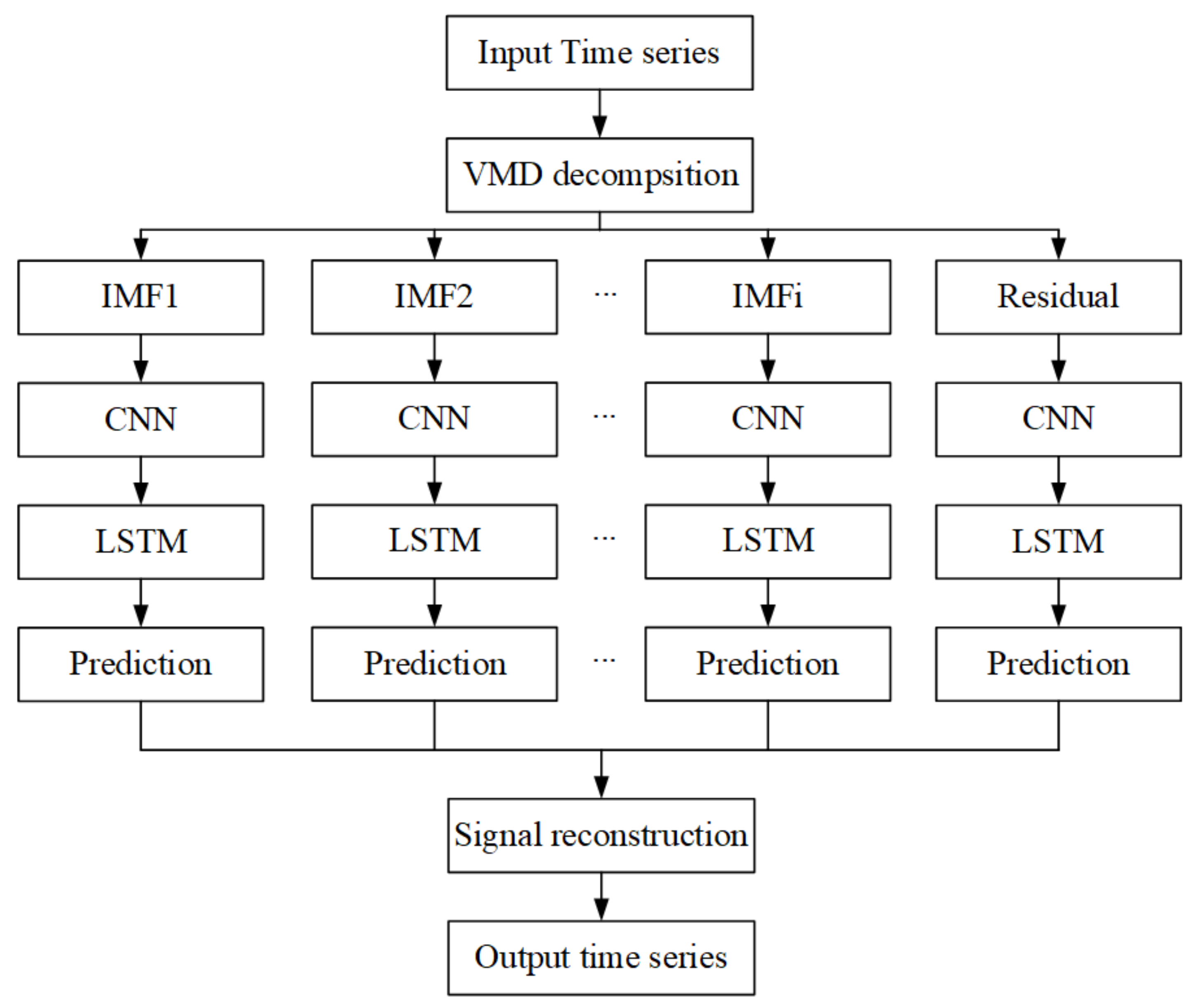
Figure 1. The proposed schemes for data processing.
Remotesensing 16 01767 g001
Figure 2. The schematic diagram of the VMD method.
Remotesensing 16 01767 g002
Figure 3. The schematic diagram of the CNN method.
Remotesensing 16 01767 g003
Figure 4. The schematic diagram of the LSTM method [44].
Remotesensing 16 01767 g004
Figure 5. The figures of the monitoring site (a,b) and the reference site (c).
Remotesensing 16 01767 g005
Figure 6. The training loss function diagram of the CNN–LSTM method.
Remotesensing 16 01767 g006
Figure 7. The prediction diagram of the CNN–LSTM method.
Remotesensing 16 01767 g007
Figure 8. VMD decomposition diagram of the original GNSS time series.
Remotesensing 16 01767 g008
Figure 9. The training loss function diagram of IMF1.
Remotesensing 16 01767 g009
Figure 10. The prediction diagram of IMF1.
Remotesensing 16 01767 g010
Figure 11. The training loss function diagram of IMF2.
Remotesensing 16 01767 g011
Figure 12. The prediction diagram of IMF2.
Remotesensing 16 01767 g012
Figure 13. The training loss function diagram of IMF3.
Remotesensing 16 01767 g013
Figure 14. The prediction diagram of IMF3.
Remotesensing 16 01767 g014
Figure 15. The training loss function diagram of IMF4.
Remotesensing 16 01767 g015
Figure 16. The prediction diagram of IMF4.
Remotesensing 16 01767 g016
Figure 17. The training loss function diagram of IMF5.
Remotesensing 16 01767 g017
Figure 18. The prediction diagram of IMF5.
Remotesensing 16 01767 g018
Figure 19. The prediction diagram of the VMD-CNN-LSTM method.
Remotesensing 16 01767 g019
Figure 20. Error histogram of CNN–LSTM (left) and VMD-CNN-LSTM (right).
Remotesensing 16 01767 g020
Figure 21. The monitoring site used for the comparative experiment from different perspectives (a) view from the left side and (b) right side.
Remotesensing 16 01767 g021
Figure 22. The prediction diagram of the VMD-CNN-LSTM and EKF methods.
Remotesensing 16 01767 g022
Table 1. The configuration parameters of the feasibility experiment.
ConfigurationParameter
The experiment period10 September 2023–21 February 2024
GNSS systems BDS(B1I, B2I), Galileo(E1B/C, E5b), GPS(L1C/A, L2C)
Sampling frequency1 Hz
Ambiguity resolution methodMLAMBDA
Multipath error modelStellar day filter in observational domain
Troposphere methodSaastamoinen model + random walk
Ionosphere methodBroadcast model
Intervals of outputs1 h
Smoothing filter methodRauch–Tung–Striebel smoother filtering method
Table 2. The comparison of the IMFs’ prediction accuracy.
MSE (mm)RMSE (mm)MAE (mm)R2
IMF10.00650.08090.0724−0.6943
IMF22.852 × 10−50.00530.00420.9988
IMF30.00020.01340.01070.9530
IMF46.9622 × 10−60.00260.00200.6527
IMF54.3939 × 10−60.00210.00170.6078
Table 3. The comparison of the VMD-CNN-LSTM and the EKF.
MSE (mm)RMSE (mm)MAE (mm)R2
EKF0.16460.40570.32360.9037
VMD-CNN-LSTM0.05410.23260.18330.9654
Disclaimer/Publisher’s Note: The statements, opinions and data contained in all publications are solely those of the individual author(s) and contributor(s) and not of MDPI and/or the editor(s). MDPI and/or the editor(s) disclaim responsibility for any injury to people or property resulting from any ideas, methods, instructions or products referred to in the content.