An Autonomous Global Star Identification Algorithm Based on the Fast MST Index and Robust Multi-Order CCA Pattern

Abstract

Star identification plays a key role in spacecraft attitude measurement. Currently, most star identification algorithms tend to perform well only in a scene without noise and are highly sensitive to noise. To solve this problem, this paper proposes a star identification algorithm based on the maximum spanning tree (MST) index and multi-order continuous cycle angle (CCA) intended for the lost-in-space mode. In addition, a neighboring star selection method named dynamic eight-quadrant (DEQ) is developed. First, the DEQ method is used to select high-confidence neighboring stars for the main star. Then, the star image is regarded as a graph, and the Prim algorithm is employed to construct the MST pattern for each guide star, which is then combined with the K vector index to perform the main star candidate search. Finally, the Jackard similarity voting for the multi-order CCA of the main star is used to identify the main star, and the global neighboring star identification is conducted by the multi-order CCA of neighboring stars. The simulated and real star images test results show that compared with five mainstream algorithms, when the position noise is 1 pixel, the number of false stars is five, the magnitude noise is 0.5, and the identification accuracy of the proposed algorithm is higher than 98.5%. Therefore, the proposed algorithm has excellent anti-noise ability in comparison to other algorithms.

1. Introduction

The measurement of spacecraft attitude refers to determining the orientation of the spacecraft in the inertial coordinate system. This task plays a key role in the fields of astronomical navigation, remote sensing observation, and deep space exploration missions. In recent years, there have been many examples of fatal problems in satellites due to the incorrect operation of the attitude determination system, and a typical one is: “Lewis spacecraft spins out of control [1].” Therefore, the attitude determination system has been considered a vital subsystem in space missions [2]. The most critical component in the attitude determination system is an aerospace attitude sensor. At present, the commonly used aerospace attitude sensors mainly include sun sensors, infrared horizon sensors, gyroscopes, and star sensors. Compared with the other types of sensors, the star sensor provides more accurate three-axis attitude data in terms of arc seconds and can output attitude without knowing the prior attitude [3]. Due to the mentioned advantages, currently, a star sensor is the most widely used type of aerospace attitude sensor [4].

The workflow of a star sensor mainly includes two stages: offline and online. The offline stage is to load the star pattern database (SPD) on the ground. In contrast, the online stage mainly includes three steps: on-orbit centroid extraction, star identification, and attitude calculation. In addition, a star sensor has two operational modes: lost-in-space (LIS) mode and tracking mode [5]. The LIS mode occurs when there is no prior attitude or the attitude data are lost due to a malfunction [6]. In such a case, the star identification in the full-sky area is performed to determine the initial attitude, but this has high requirements for the robustness and real-time performance of a star identification algorithm. Then, a sensor enters the tracking mode and starts the star searching and identification process in a local area using the initial attitude data. Thus, star identification in the LIS mode is more challenging than that in the tracking mode.

In a realistic space deployment scenario, there can be certain deviations between the captured images and pre-stored guide stars in some boresight directions, which can have a severe impact on the star identification result. The main reasons for these deviations may be due to the following: the interference stars appear on the imaging plane due to radiation from nearby planets and space debris, causing the false star noise; the interference of the internal circuit of a star sensor might lead to high-magnitude star missing, which represents the magnitude noise; the focal length and principal point calibration errors of a star sensor and the jitter of a satellite platform can lead to a deviation in the star imaging position, resulting in the position noise. The listed cases have a high possibility of causing a star identification failure. Therefore, fast and accurate star identification in the LIS mode is extremely challenging, and many star identification algorithms have been proposed in recent years. Generally, the mainstream star identification algorithms can be divided into three categories: the subgraph-based class, pattern-based class, and learning class [7,8,9,10,11]. Typical, recently published star identification algorithms of three different categories are listed in Table 1.

Table 1. Classification of mainstream star identification algorithms.

Algorithm	Category	Methodology
Sun et al. [12]	Subgraph-based	Double-triangle with the star angle and distance
Liu et al. [13]	Subgraph-based	Triangle voting scheme
Kolomenkin et al. [14]	Subgraph-based	Geometric voting strategy
Mortari et al. [15]	Subgraph-based	Pyramid structure and K vector search
Cole et al. [16]	Subgraph-based	Area and polar moments of triangles
Lee et al. [17]	Pattern-based	Polar grid and multi-reference stars
Li et al. [18]	Pattern-based	Two-dimensional angular distances
Aghaei et al. [19]	Pattern-based	Optimization method
Zhang et al. [20]	Pattern-based	Radial and cyclic pattern
Samirbhai et al. [21]	Pattern-based	Rotation-invariant 2D vector
Jiang et al. [22]	Pattern-based	Redundant-coded star pattern
Liu et al. [23]	Pattern-based	A priori algorithm
Jiang et al. [4]	Learning-based	Hierarchical convolutional neural network (CNN)
Yang et al. [9]	Learning-based	1D-CNN

The so-called subgraph-based algorithms use a geometric structure between the stars to identify stars. The SPD is regarded as a graph, and the captured image is regarded as a subgraph, where graph vertices denote stars, and graph edges represent angular distances between the stars. Thereafter, the star identification is realized through the correspondence of vertices and edges between the subgraph and the SPD. The most classical algorithm of this type is the triangle algorithm [24], which regards the three brightest stars in the field of view (FOV) as vertices and angular distances between every two vertices as three edges of a triangle, thus constructing a unique triangle. This algorithm is simple and has been one of the most commonly used algorithms in engineering. However, it has the disadvantage of low feature dimensions, which makes redundant matching prone to occur. In addition, as the detection capability of a star sensor increases, the SPD memory increases exponentially, resulting in a significant decrease in search efficiency. Aiming to solve the aforementioned problems, recent research has proposed many triangle-derived algorithms [12,13,14,15,16], of which the most representative is the pyramid algorithm [15] that has been successfully applied to the High-Energy Transient Explorer (HETE) task. In this algorithm, four stars are used to form a pyramid structure, and the feature dimension is improved, reducing the probability of redundant matching. Furthermore, the K vector algorithm was introduced, which greatly improves search efficiency. In [14], the authors developed a voting strategy based on the relationship between stars to vote, but the identification accuracy decreased significantly with the number of false stars. In view of that, in [13], the authors proposed a multi-layer voting algorithm, which can slightly improve the anti-noise ability, but its SPD storage is large. Overall, the subgraph-based algorithms generally face the problem of large SPD storage memory.

Compared with the subgraph-based algorithms, the pattern-based algorithms typically have a smaller SPD. The first proposed algorithm of this type was the grid algorithm [25,26], which aims to construct a unique star pattern based on the positional relationship between the main star and the nearest neighboring star, called the reference star. However, due to over-reliance on the reference star, the identification accuracy decreases rapidly when there is noise interference. On this basis, many improved algorithms were derived [17,18,19,27]. For instance, in [17], a grid pattern vector in the polar grid was constructed, and a multi-reference stars method was proposed, but the problems of dependence on the reference star and high sensitivity to noise remained unsolved. In [18], the authors used a two-dimensional angular distance pattern to replace the original grid pattern and combined the traversal method to determine the reference star, which improved the robustness to noise. However, the traversal method has high computational complexity, resulting in reduced real-time performance. In addition, a series of algorithms for circular and radial patterns were developed [20,22,28]. In [22], an algorithm combining radial and neighboring star patterns was proposed, and redundant coding was used for storage, which reduced the storage capacity of the SPD. Further, in [23], companion stars were determined by the a priori algorithm, and a radial pattern image was generated, but only the selected neighboring stars could be identified. In [21], an innovative rotation-invariant two-dimensional vector pattern was designed; this design is robust against the positional noise, but its identification accuracy drops rapidly with the number of false stars. In [29], a combination of hamming distance and spearman correlation was adopted for star identification. However, this approach could identify only one to two stars adjacent to the main star. The general disadvantage of the pattern-based algorithms is that most of them perform poorly under the aforementioned three types of noises and cannot achieve global star identification.

Learning-based algorithms essentially represent a class of pattern-based algorithms [30]. Since CNN was applied to star identification [31], many CNN-based algorithms for star identification have been proposed, and the most representative ones use spider-web images and hierarchical CNN [4], mixed star patterns and multi-layer SOM neural networks [32], and 1D CNN [9]. They input the constructed patterns or star images into the network for training to classify and identify the guide stars in a captured star image. Although this kind of algorithm can improve the identification accuracy, the iterative updating of network weights results in a long running time. In addition, the memory consumption of learning-based algorithms is generally large.

Through the aforementioned analysis, it is found that star identification mainly has the disadvantages of a long running time, large memory usage, and sensitivity to noise. In this paper, with reference to pattern-based algorithms, a global star identification algorithm based on the maximum spanning tree fast index and continuous cycle angle is proposed, which greatly improves the search time and anti-noise ability of pattern-based star identification.

The main contributions of this study can be summarized as follows:

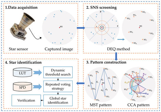
• A dynamic eight-quadrant method for neighboring stars selection, which makes the guide stars in the FOV uniformly distributed and increases the identifiability of the constructed pattern, is proposed. This provides a novel idea for the selection of neighboring stars;
• The Prim algorithm is introduced into the field of star identification first, constructing the maximum spanning tree pattern for each main star, and is then combined with the K vector to define a fast index, which greatly improves the search efficiency of the main star;
• A multi-order continuous cycle angle pattern is designed and used to perform the global identification of neighboring stars, which improves the anti-noise performance of the pattern-based algorithm;
• Extensive experiments are conducted on simulated and real star images, and the experimental results show that the proposed algorithm is superior to most mainstream algorithms in terms of identification accuracy, memory, and time consumption.

The rest of this paper is organized as follows. Section 2 introduces the pre-knowledge and pattern framework. Section 3 presents the proposed algorithm, including the strategies for LUT, SPD generation, and star identification. Section 4 compares the proposed algorithm with five mainstream algorithms. Section 5 discusses the advantages and limitations of this study. Finally, Section 6 concludes this study. Appendix A summarizes all the abbreviations used in the study.

2. Pre-Knowledge and Pattern Framework

2.1. Pre-Knowledge

This section briefly introduces the terms involved in this study.

Guide star catalog: The original star catalog used in this study is the Smithsonian Astrophysical Observatory (SAO) star catalog, which contains 258,997 stars with a magnitude dimmer than 11 and includes data on the right ascension (α_i), declination (β_i), apparent magnitude, and other astronomical parameters of each star [33]. According to the detection capability of the star sensor used in this study, the stars with a magnitude below 6 are selected to form the guide star catalog, and a two-dimensional distribution graph is drawn according to the position coordinates (α_i,β_i) of the selected stars, as shown in Figure 1.

Figure 1. The two-dimensional distribution of the guide stars with a magnitude lower than 6.

Star sensor: The model diagram of the star sensor imaging the stars on the imaging plane is shown in Figure 2, where the reddish-brown star represents the main star (MS) in the current FOV, the blue star represents the star in the FOV but not selected as neighboring star (NS), the orange star represents the star selected as NS, and the number of NSs is denoted by N; the orange stars represent other stars in the celestial sphere, and A_ij is the angular distance between stars i and j.

Figure 2. The illustration of the star imaging process by the star sensor.

Continuous cyclic angle: The maximum FOV radius is denoted by PR_max, and the continuous cyclic angle (CCA) is defined as an angle between the lines connecting the MS and any two NSs in the FOV. The CCA for N = 8 is presented in Figure 3; Figure 3a shows the angle between the adjacent NSs, denoted by ${\theta }_i$ (i = 1, 2, ..., N), which represents the first-order CCA pattern of an NS; Figure 3b shows the multi-order CCA pattern of ${\mathrm{NS}}_1$, denoted by ${\theta }_{1,m}$ (m = 2, 3, …, N). Among them, ${\theta }_{1,2}={\theta }_1$, ${\theta }_{1,3}={\theta }_1+{\theta }_2$, …, ${\theta }_{1,8}={\theta }_1+{\theta }_2+{\theta }_3+{\theta }_4+{\theta }_5+{\theta }_6+{\theta }_7$. The CCAs of other orders of ${\mathrm{NS}}_1$ are calculated in the same way. Similarly, the multi-order CCA patterns of other NSs are constructed.

Figure 3. Schematic diagram of the multi-order CCA construction process. (a) First-order CCA of all NSs; (b) Multi-order CCA of ${\mathrm{NS}}_1$; (c) Multi-order CCA of ${\mathrm{NS}}_8$.

Graph structure: A star image is regarded as an undirected graph in this study; namely, all stars are regarded as a vertex set (V) of graphs (G), and all inter-star connections are regarded as an edge set (E); the Euclidean distance of E is regarded as an edge weight. The maximum spanning tree (MST) represents the set of the maximum edge weights that connect all vertices without loops, and it can be represented by a set$\mathrm{T}=\left\{d\right(u,v\left)\right|(u,v) \in V\}$, where $d(u,v)$ represents the edge weight for the MST. Therefore, the value of MST can be calculated as $w\left(\mathrm{T}\right)={{\displaystyle \sum }}_{d(u,v)\in \mathrm{T}} d(u,v)$.

2.2. Proposed Rotation-Invariant Pattern Frames

Ideally, the star sensor should be imaged in the same position as a star when the SPD is constructed. However, in the real imaging process, it is common that a star rotates on the imaging plane, and constructing a rotation-invariant pattern is the primary task in the star identification algorithm design.

In this study, a multi-order CCA pattern star image identification framework based on the MST fast index is proposed. The construction and identification principles of the proposed framework are explained in detail in Section 3, and in this section, the rotation invariance of the proposed framework is explained.

First, the projection transformation steps of the star sensor are analyzed. According to (α_i, β_i) of the guide star, the coordinates of the ith guide star in the earth-centered inertial (ECI) coordinate system can be expressed as follows:

$${\mathit{v}}_i^{ECI}=[X_i^{ECI};Y_i^{ECI};Z_i^{ECI}]=[\cos {\alpha }_i\cos {\beta }_i;\sin {\alpha }_i\cos {\beta }_i;\sin {\beta }_i].$$

(1)

Then, the coordinates of the ith guide star in the star sensor coordinate system are defined by:

$${\mathit{v}}_i^{sen}=[X_i^{sen};Y_i^{sen};Z_i^{sen}]=\mathit{C}\cdot {\mathit{v}}_i^{ECI},$$

(2)

where $\mathit{C}$ is the attitude rotation matrix [1], which converts the ECI coordinates ${[X}_i^{\mathit{ECI}}{, Y}_i^{\mathit{ECI}}{, Z}_i^{\mathit{ECI}}]$ to the star sensor coordinates ${[X}_i^{\mathit{sen}}{, Y}_i^{\mathit{sen}}{, Z}_i^{\mathit{sen}}]$.

Finally, the coordinates of the ith guide star on the imaging plane ${(x}_i{, y}_i)$ are calculated by:

$$\{\begin{array}{l}{x}_i=\frac{f{X}_i^{sen}}{p_x{Z}_i^{sen}}+\frac{D_x}{2}\\ y_i=\frac{f{Y}_i^{sen}}{p_y{Z}_i^{sen}}+\frac{D_y}{2}\end{array},f=\frac{D_x{p}_x}{2\tan (\frac{FO{V}_x}{2})}=\frac{D_y{p}_y}{2\tan (\frac{FO{V}_y}{2})},$$

(3)

where $p_x{, D}_x$, and ${\mathit{FOV}}_x$ denote the pixel size, the number of pixels, and the degree of FOV in the x-dimension, respectively; the meaning of the parameters in the y-dimension is the same.

Next, the rotation invariance analysis of the CCA pattern is performed. The first-order CCA of all NSs is expressed as follows:

$${\theta }_i=\{\begin{array}{l}\left[\arccos (\frac{dot((x_i-x_m,y_i-y_c),(x_{i+1}-x_m,y_{i+1}-y_m))}{\left|\right|x_i-x_m,y_i-y_m|{|}_2\cdot ||x_{i+1}-x_m,y_{i+1}-y_m|{|}_2})\right],i=1,\dots ,N-1,\\ \left[\arccos (\frac{dot((x_N-x_m,y_N-y_m),(x_1-x_m,y_1-y_m))}{\left|\right|x_N-x_m,y_N-y_m|{|}_2\cdot ||x_1-x_m,y_1-y_m|{|}_2})\right],i=N,\end{array}$$

(4)

where ${(x}_i{, y}_i)$ are the coordinates of the ith NS on the imaging plane, and ${(x}_m{, y}_m)$ are the coordinates of the MS of the imaging plane; function dot(${\mathit{b}}_1$,${\mathit{b}}_2$) returns the dot product of vectors ${\mathit{b}}_1$ and ${\mathit{b}}_2$; $\left|\right|·{\left|\right|}_2$ represents the two-norm of a vector; $[·]$ indicates rounding to the nearest integer.

Assume that $\mathit{S}=\left[{\theta }_1,{\theta }_2,\dots ,{\theta }_N\right],$ which represents the first-order CCA set; then, according to the CCA definition and Equation (4), the ith NS multi-order CCA pattern of the kth MS can be expressed as follows:

$$\begin{array}{l}{\mathit{A}}^k[i]=[{\mathit{S}}_i,{\mathit{S}}_i+{\mathit{S}}_{i>>1},\dots ,{\mathit{S}}_i+{\mathit{S}}_{i>>1}+\dots +{\mathit{S}}_{i>>(N-1)}],\\ s.t.\hspace{1em}1<i\le N\end{array}$$

(5)

where the symbol “>>” means that vector S is shifted circularly to the right.

Further, define the matrix consisting of ${ \mathit{A}}^k\left[i\right] (i=1, 2,\dots , N)$ as a multi-order CCA pattern of the kth MS as follows:

$${\mathit{A}}^k=[{\mathit{A}}^k[1];{\mathit{A}}^k[2];\dots ;{\mathit{A}}^k[N]],$$

(6)

where the rows in ${\mathit{A}}^k$ represent the ${ \mathit{A}}^k\left[i\right] (i=1, 2,\dots , N)$ of NSs, and the columns denote the zth-order CCA patterns, where $\mathrm{z}=1, 2,\dots , N – 1$.

As a star sensor rotates, the imaging plane coordinates of stars change. According to Equation (4), the rotated first-order CCA can be expressed by:

$${\theta }_i^{R_{\delta }}=\{\begin{array}{l}\left[\arccos (\frac{R_{\delta }\cdot dot((x_i-x_m,y_i-y_m),(x_{i+1}-x_m,y_{i+1}-y_m))}{\sqrt{R_{\delta }}\cdot \sqrt{R_{\delta }}\cdot \left|\right|x_i-x_m,y_i-y_m|{|}_2\cdot ||x_{i+1}-x_m,y_{i+1}-y_m|{|}_2})\right],i=1,\dots ,N-1,\\ \left[\arccos (\frac{R_{\delta }\cdot dot((x_N-x_m,y_N-y_m),(x_1-x_m,y_1-y_m))}{\sqrt{R_{\delta }}\cdot \sqrt{R_{\delta }}\cdot \left|\right|x_N-x_m,y_N-y_m|{|}_2\cdot ||x_1-x_m,y_1-y_m|{|}_2})\right],i=N,\end{array}$$

(7)

where $R_{\mathsf{\delta }}$ denotes the rotation matrix obtained after the rotation by angle$\mathsf{\delta }$, and it is given by:

$$R_{\delta }=\left[\begin{array}{cc}\cos \delta & -\sin \delta \\ \sin \delta & \cos \delta \end{array}\right].$$

(8)

Based on Equations (4) and (7), it holds that ${\theta }_i={\theta }_i^{R_{\mathsf{\delta }}}$. This shows that the first-order CCA set S$=\left[{\theta }_1,{\theta }_2,\dots ,{\theta }_N\right]$ does not change with rotation, while the multi-order CCA matrix ${ \mathit{A}}^k$ is constructed based on the set S, so its value is also unchanged. Thus, the rotation changes only the row order of the pattern matrix ${\mathit{A}}^k$, while its value remains unchanged and can be considered rotation-invariant. The row alignment is described in Section 3.2.

Finally, the MST construction only uses the Euclidean distance of stars on the imaging plane. According to the MST definition given in Section 2.1 and the construction process presented in Section 3.1.2, the MST pattern is also rotation-invariant. Therefore, both patterns constructed in this study are rotation-invariant. In addition, the proposed dynamic eight-quadrant NS selection method ensures the invariance of the star pattern, which is explained in Section 3.1.1.

3. Proposed Methodology

Inspired by the pattern-based algorithms, this study proposes an innovative star identification algorithm based on the MST fast index and multi-order CCA pattern. In addition, this study develops a guide star selection method named the DEQ method, which can make the guide stars in the FOV more uniform, thus ensuring the pattern is more identifiable. The proposed algorithm includes two main tasks: offline LUT and SPD generation and online star identification. The specific steps of the proposed algorithm are as follows. In the offline step, each star at the center of the FOV is denoted as MS, a unique MST look-up table (LUT) index is constructed, and a multi-order CCA pattern is generated to obtain the SPD. In the online step, both patterns are constructed from the captured or simulated images. First, the candidate MS set is obtained using the K vector value from the LUT, and then the unique MS and NSs in the image are identified based on the CCA pattern. The flowchart of the proposed algorithm is shown in Figure 4, where DMS and DNS represent the MS and NS of the LUT and SPD, respectively; SMS and SNS denote the MS and NS of the captured and simulated images, respectively. In Figure 4, the upper and lower structures represent two major steps, and the right side presents the rough flow of the proposed global star identification.

Figure 4. The flowchart of the proposed algorithm consisting of the offline and online steps.

3.1. LUT and SPD Generation

Before constructing the offline LUT and SPD, it is necessary to preprocess the guide star catalog, which includes performing magnitude filtering and double star merging [34] and then obtaining $N_s$= 4956 stars. Next, the LUT and SPD construction steps are conducted. Generally, if the number of stars in the FOV is too small, the star identification will fail; in contrast, if the number of stars in the FOV is too large, the star pattern will be redundant, which will also cause identification errors. Therefore, it is essential to select an optimal number of stars before constructing the star pattern. The number of stars in different FOVs is presented in Figure 5, where it can be seen that there are redundant stars in most of the boresight for FOV = 20° × 20°. To solve this problem, this study proposes a dynamic eight-quadrant NS selection method named the DEQ method. The NSs selected by the DEQ method are more uniformly distributed in the FOV, which makes the constructed patterns more identifiable.

Figure 5. The distribution of star numbers for different FOVs.

3.1.1. DEQ Method

The DEQ method involves two main steps: eight-quadrant division and dynamic soft interval select ${\mathrm{DNS}}_i^k$, which are explained in the following.

Step 1: Eight-quadrant division: In the guide star catalog, place each star in the center of the FOV in turn and select the center star as the ${\mathrm{DMS}}^k \left(k=1, 2, \dots , N_s\right)$ each time, which is denoted by reddish-brown in Figure 6a. Then, set the minimum field radius PR_min = 0.1°, avoiding selecting a ${\mathrm{DNS}}_i^k$ (i = 1, …, N) that is too close to the ${\mathrm{DMS}}^k$. Further, initialize the dynamic radius PR_d, as shown in Figure 6b. Based on the x and y axes and the diagonal direction, the eight quadrants are divided, as shown in Figure 6c;

Figure 6. The NS selection rules in the proposed DEQ method. (a) Distribution of redundant NSs in the FOV; (b) Parameter settings; (c) Eight-quadrant division based on the imaging plane coordinate system; (d) According to ${\lambda }_i$ of the stars in each quadrant, a dynamic NS selection is performed.

Step 2: Dynamic soft interval select ${\mathrm{DNS}}_i^k$: First, set an initial value of g to make PR_d change dynamically within (PR_min, PR_max), where PR_max is FOV/2, as shown in Figure 6d. Moreover, denote the maximum number of $\mathrm{DNSs}$ by N_max. The values of N_max and g and the initial value of PR_d are given in Table 2. The parameter N_max is to ensure that there is a guide star in each quadrant in most boresight directions; therefore, the value is set to eight. By randomly generating 10,000 boresight directions, most of the guide stars under the FOV = 20° × 20° are distributed within the FOV with a radius of 5°, so PR_d = 5° is set; moreover, it is set to g = 1.25°. When the FOV radius of 5° does not meet the aforementioned distributions, then it can be satisfied after one or two iterations.

Table 2. Parameter settings of the DEQ method.

Parameters	Illustration	Value
$N_{\mathit{max}}$	Maximum number of NSs	8
g	Dynamic step size	1.25 (deg)
$P_d$	Initial radius	5 (deg)

Next, the process of the DEQ method is explained in detail.

In this study, the confidence factor λ_i is defined for each ${\mathrm{DNS}}_i^k$ by Equation (9), which served as an NS selection criterion for each quadrant.

$${\lambda }_i=- (\frac{Ma{g}_i-Ma{g}_{min}}{Ma{g}_{max}-Ma{g}_{min}}+\frac{r_i}{d_{max}}\ast 2),$$

(9)

where ${\mathit{Mag}}_i$ and $r_i$ are the magnitude and the Euclidean distance from the center of the ith star, respectively; Mag_min and Mag_max are the minimum and maximum magnitudes, respectively; $d_{\mathit{max}}=\sqrt{{D_x}^2+{D_y}^2}$ is the maximum imaging plane distance.

Next, select a star from each of the eight quadrants in the range (PR_min, PR_d). The process is as follows: according to the definition of ${\lambda }_i$, the lower the ${\mathit{Mag}}_i$ and $r_i$, the larger the ${\lambda }_i$ value is, and the easier it is for a star to be selected as ${\mathrm{DNS}}_i^k$. Thus, the DNS with the largest ${\lambda }_i$ value in each quadrant is selected, as shown in Figure 6d. When the number of selected DNSs is less than N_max, PR_d is incremented by g to increase the field range; this process is repeated until PR_d = PR_max to meet the condition that there is a star in all eight quadrants, which is defined as the eight-quadrant distribution. However, for sky areas with a small number of stars, if the number of stars does not meet the eight-quadrant distribution, the stars are directly arranged according to the descending order of ${\lambda }_i$, and the top N_max stars are selected as DNSs. Compared to the direct selection of the brightest N_max stars in the FOV, which represents the BR method, or N_max stars closest to the DMS, which is the ED method, the proposed DEQ method can effectively reduce the noise interference caused by missing and false stars and position deviation. The performance of the proposed DEQ method is demonstrated in Section 4.1.

3.1.2. MST and CCA Pattern Construction

In the proposed DEQ method, a uniform distribution and a relatively fixed number of DNSs are selected for each ${\mathrm{DMS}}^k$, which paves the way for the construction of more identifiable MST and CCA patterns.

The first step is based on the LUT of MST, which is to index the candidate MSs to speed up the star identification process. As mentioned in Section 2.1, stars captured by a star sensor are regarded as a vertex of G, and the weight between two vertices (u,v) is defined as their Euclidean distance on the imaging plane, which is calculated by:

$$\begin{array}{l}d(u,v)=\sqrt{{(x_u-x_v)}^2+{(y_u-y_v)}^2},\\ s.t. u,v\in \mathrm{V}\end{array}$$

(10)

where ${(x}_u{, y}_u)$ and ${(x}_v{, y}_v)$are the coordinates of the two stars on the imaging plane.

Next, the MST pattern is constructed. There are two commonly used algorithms for MST construction: the Kruskal algorithm and the Prim algorithm. Among them, the Kruskal algorithm is more suitable for sparse graphs, whereas the Prim algorithm is more appropriate for dense graphs [35]. The general judgment principle for dense and sparse graphs is defined as follows:

$$\{\begin{array}{l}{L}_E\ge L_V\ast \log L_V, \mathrm{dense} \mathrm{graphs}, \\ \mathrm{otherwise}, \mathrm{sparse} \mathrm{graphs}, \end{array}$$

(11)

where $L_E$ represents the number of edges, and $L_V$ represents the number of vertices.

In this study, the number of vertices represents the number of stars in the FOV after screening by the DEQ method, that is, $L_V=N+1=9$. Considering the edge weights between all stars in the FOV, there are nine vertices, with $L_E{=\mathrm{C}}_9^2=36$ edges. After substituting $L_V$ and $L_E$ into Equation (11), it can be concluded that this problem belongs to the MST construction problem of dense graphs. Therefore, this study uses the Prim algorithm for the MST pattern construction of each guide star.

The detailed steps of the MST index construction process are as follows. First, define V = {${\mathrm{NS}}_1{, \mathrm{NS}}_2{, \mathrm{NS}}_3{, \mathrm{NS}}_4{, \mathrm{MS}, \mathrm{NS}}_5{, \mathrm{NS}}_6{, \mathrm{NS}}_7{, \mathrm{NS}}_8$} as a set of all vertices and U as a set of MST vertices. Randomly select a star from the guide stars selected in the eight quadrants as a starting point (i.e., ${\mathrm{NS}}_3$ in Figure 7a), use Equation (10) to calculate the distance between it and other stars as an edge weight, and select the maximum edge weight value as $r_1$, as shown in Figure 7b. In addition, the vertex of MST is denoted by U = {${\mathrm{NS}}_3{, \mathrm{NS}}_6$}. Then, select the edge with the largest weight from all edges connected with ${\mathrm{NS}}_3$and ${\mathrm{NS}}_6$as the second edge $r_2$, as shown in Figure 7c; then, the MST vertex is expressed by U = {${\mathrm{NS}}_2{, \mathrm{NS}}_3{, \mathrm{NS}}_6$}. According to the aforementioned steps and the rule that any three vertices cannot form a loop, when all nine vertices are selected as MST vertices, the MST pattern construction of the ${\mathrm{DMS}}^k$ is completed, as shown in Figure 7d. The final MST pattern calculation is given by:

$$w_D(T^k)={\displaystyle \sum _{i=1}^N{d}_i(u,v)}.$$

(12)

Figure 7. The MST pattern construction steps when the Prim algorithm is used. (a) Randomly select the starting vertex (${\mathrm{NS}}_3$) and calculate the Euclidean distance to the other stars; (b) Select the edge with the largest distance as a weight of the first edge ($r_1$); (c) Select another vertex (${\mathrm{NS}}_6$) connected to $r_1$ as the second vertex; similarly, select the weight of the second edge ($r_2$); (d) Construct the eight maximum edge weights.

After obtaining the MST pattern of each MS, store the generated patterns in a one-dimensional vector Y with a length of $N_s$, denoted by ${\mathbf{Y}\left(k\right)=\{\mathrm{w}}_{\mathrm{D}}{(\mathrm{T}}^1{), \mathrm{w}}_{\mathrm{D}}{(\mathrm{T}}^2{), \dots , \mathrm{w}}_{\mathrm{D}}{(\mathrm{T}}^{N_s}\left)\right\}$. In addition, to increase the search efficiency of the MST candidate MS, the K vector algorithm is used to locate the search interval rapidly. Namely, it takes only a few simple steps to perform interval indexing fast, and the corresponding time complexity is O(1).

The specific steps in combining the K vector with the MST are as follows:

(1)

Arrange vector Y in ascending order, that is, Y(1) =${ \mathrm{Y}}_{\mathit{min}}$, $\mathrm{Y}\left(N_s\right){=\mathrm{Y}}_{\mathit{max}}$. The average step size occupied by each element in vector Y is $L_d=(\mathrm{Y}\left(N_s\right){ - \mathrm{Y}\left(1\right))/(N}_s- 1)$. Mortari et al. [15] pointed out that the straight line connecting (1, Y(1) − $L_d/2$), ($N_s$, Y($N_s$) + $L_d/2$) can ensure that each step contains Y(k). Therefore, a straight line y(x) is drawn according to the vector Y, which can be expressed as follows:

$$\{\begin{array}{l}y(x)=a_{1}x+a_0,\\ a_1=\frac{\mathrm{Y}(N_s)-\mathrm{Y}(1)+L_d}{N_s-1},\\ a_0=\mathrm{Y}(1)-a_1-L_d/2.\end{array}$$

(13)

(2)

Define the K vector index function K(x) as follows:

$$\{\begin{array}{l}\mathrm{K}(x)=k,\\ \mathrm{Y}(k)<y(x)<\mathrm{Y}(k+1),\end{array}$$

(14)

where k is the serial number of ${\mathrm{DMS}}^k$ in the LUT, and x is the MST index value.

Next, the CCA pattern in the SPD is constructed. The CCA definition is introduced in Section 2.1; therefore, in this section, only the construction process is presented. First, the first-order CCA set that is shown in Figure 8a is denoted as $\mathbf{S}=\left[{\theta }_1,{\theta }_2,\dots ,{\theta }_N\right]$, and the corresponding calculation formula is given in Equation (4). The ${\mathrm{DMS}}^k$ multi-order CCA of the ith ${\mathrm{DNS}}_i^k$ (i = 1, 2, …, N) is calculated by Equations (5) and (6). The multi-order CCA construction process of eight NSs is presented in Figure 8b,c, where ${\theta }_{uv}$ represents the counterclockwise angle between the vertices u and v; for instance, ${\theta }_{85}={\theta }_8+{\theta }_1+{\theta }_2+{\theta }_3+{\theta }_4$. The multi-order CCA pattern of the ${\mathrm{DMS}}^k$ is presented in Figure 8d, and it is used to select the correct MS from the candidate DMS set obtained by the MST if the candidate star obtained by the MST is not unique, as well as to identify NSs. The multi-order CCA of each ${\mathrm{DMS}}^k$ is an N × (N – 1) matrix, where each column denotes the CCA pattern of ${\mathrm{DMS}}^k$ from the first order to the (N – 1)th order, which is used to obtain the correct MS from the candidate DMS set; each row in the matrix represents the multi-order CCA of ${\mathrm{DNS}}_i^k$, which is used to identify NSs. After obtaining the correct MS, the row identification can be directly performed to obtain the correct NS. The identification process is described in detail in Section 3.2.

Figure 8. The multi-order CCA pattern construction process of ${\mathrm{DMS}}^k$. (a) The first-order CCA of ${\mathrm{NS}}_1$–${\mathrm{NS}}_8$; (b) The multi-order CCA of ${\mathrm{NS}}_1$; (c) The multi-order CCA of ${\mathrm{NS}}_8$; (d) The multi-order CCA pattern of ${\mathrm{DMS}}^k$.

Finally, the storage format of the guide star catalog, including the LUT and SPD, is shown in Figure 9. The LUT is stored in an increasing order of MST, and the multi-order CCA of each ${\mathrm{DMS}}^k$ is stored in the ${\mathrm{DNS}}_i^k$ counterclockwise order. The storage content mainly includes the star number (k), right ascension (${\mathsf{\alpha }}_k$), declination (${\mathsf{\beta }}_k$), and magnitude of stars. In addition, MST and CCA patterns for each star are included, which are stored in LUTs and SPDs, respectively. Among them, each row in the LUT corresponds to a main star, which is used to rapidly search for candidate DMSs; the SPD stores the CCA pattern matrix of each star, and the meaning of its row and column has been indicated in Figure 9, which is used to realize the determination of the unique DMS and the global SNSs identification.

Figure 9. The storage format of the guide star catalog, including the LUT and SPD. (a) Parameters stored in the guide star catalog; (b) The LUT storage format used to obtain the candidate DMS set; (c) The SPD storage format used to obtain the correct ${\mathrm{DMS}}^k$ and identify ${\mathrm{SNS}}_i^k$.

3.2. Star Identification Scheme

To identify the SMS and SNSs rapidly and accurately after screening by the DEQ method, this study proposes a two-step identification method. First, the star coordinates in the captured image are extracted and shifted to the image center, and the SNSs are selected using the DEQ method. Then, the selected guide stars are used to generate the MST pattern and combined with the K vector algorithm to establish an indexing mechanism for the rapid locating of DMS candidates from the LUT. Next, the correct SMS and its SNSs are identified from the DMS candidate set by voting using the Jaccard similarity coefficients of each order CCA pattern. Finally, the identified stars are verified to eliminate mismatched stars. The identification framework is shown in Figure 10.

Figure 10. The overall identification framework.

The specific steps of the identification algorithm are as follows:

Step 1: SMS selection

In real scenes, it cannot be guaranteed that there is a guide star in every FOV center. Therefore, when a star image frame is to be identified and captured, the centroid extraction algorithm is used first to calculate the 2D coordinates of each star in the FOV. Then, the Euclidean distance between them and the image center${(x}_c{, y}_c)$is calculated. Finally, the star with the smallest value is selected as an SMS and denoted by${(x}_m{, y}_m)$.

Step 2: SNS selection for SMS

The DEQ method is employed to perform SNSs selection. First, the 2D coordinate deviations between${(x}_c{, y}_c)$and${(x}_m{, y}_m)$in the x and y dimensions are calculated and denoted by ${\Delta x=x}_m {- x}_c{ \mathrm{and} \Delta y=y}_m{ - y}_c$, respectively. Then, translate${(x}_m{, y}_m)$to coincide with${(x}_c{, y}_c)$ following the translation rule of:

$$\{\begin{array}{l}{x^{\prime }}_m=x_m-\Delta x\\ {y^{\prime }}_m=y_m-\Delta y\end{array}.$$

(15)

The coordinates${(x}_s{, y}_s)$of other stars in the FOV are also translated according to the rule defined by Equation (15), and stars whose coordinate value is greater than PR_max after translation are eliminated. Next, the same parameters, PR_d, N_max, and g, are used to define a DEQ SNS selection rule, and the confidence factor ${\mathsf{\lambda }}_i$ of each star in each quadrant is calculated by Equation (9); the star with the maximum ${\mathsf{\lambda }}_i$ value in each quadrant is selected as an SNS. Finally, eight SNSs with a relatively uniform distribution and high confidence are selected.

Step 3: MST fast index definition and candidate DMS search

Similarly, regard the nine stars, including SMS, as graph vertices and select a starting vertex randomly; next, use the Prim algorithm to construct an MST pattern for SMS until all vertices are involved in the tree denoted by $w_{\mathit{S}}\left(T\right)$. Due to the rounding errors in the tree construction process, the initial threshold $D_{\mathit{th}}$ and the dynamic change parameter $\Delta \mathrm{D}$ are used to search for the candidate DMS from the LUT roughly and rapidly. The DMS that meets the following conditions will be stored in the candidate DMS set ${\mathsf{\Omega }}_{\mathit{candi}}$:

$$\begin{array}{l}{\mathsf{\Omega }}_{candi}=\{{\mathrm{DMS}}^k,(k=1,\dots ,N_{candi})|w_S(T)-D_{th}\le w_D(T)\le w_S(T)+D_{th}\},\\ s.t.\hspace{1em}{D}_{th}=D_{th}+l\cdot \Delta \mathrm{D},l=l+1,l\ge 0\end{array}$$

(16)

where l is the iteration number, which is used to increase the threshold interval when the correct DMS is not involved in ${\mathsf{\Omega }}_{\mathit{candi}}$, and $N_{\mathit{candi}}$is the number of candidate DMSs.

The advantage of the dynamic threshold is that it not only effectively avoids a long search time under the high threshold but also reduces the probability of missing the correct candidate star due to the too-small threshold. In this way, the search efficiency is significantly improved, while the length of ${\mathsf{\Omega }}_{\mathit{candi}}$ is effectively reduced. In this study, set $D_{\mathit{th}}$= 1 pixel and $\Delta \mathrm{D}$ = 16 pixels. This is because the maximum position noise in real scenes is approximately 1 pixel; in this case, the maximum MST pattern difference caused by the position noise is about 16 pixels.

Simultaneously, to increase the search efficiency, using the K vector algorithm to create a fast index mechanism, rapidly locate the starting and ending candidate DMS intervals. First, calculate the index value $x_{\mathit{star}}{ \mathrm{and} x}_{\mathit{end}}$ as follows:

$$\{\begin{array}{l}{x}_{start}=\frac{w_S(T)-D_{th}-a_0}{a_1},\\ x_{end}=\frac{w_S(T)+D_{th}-a_0}{a_1}.\end{array}$$

(17)

Then, substitute the index value into the K vector function, Equation (14), to obtain the serial number $(k_{\mathit{start}}{, k}_{\mathit{end}}$) of the candidate DMSs in the LUT. The obtained row corresponds to a candidate DMS; finally, store them in ${\mathsf{\Omega }}_{\mathit{candi}}.$Step 4: Multi-order CCA pattern construction for SMS and SNS identification

First, randomly select a star as a starting star and use Equations (4)–(6) to obtain the multi-order CCA pattern of the captured star image. If the number of candidate DMSs $N_{\mathit{candi}}$ is less than one, a dynamic threshold will adjust the range to obtain a new set of candidate DMSs; if $N_{\mathit{candi}}=1$, the candidate DMS is considered to be the correct MS; otherwise, the Jackard similarity coefficient of the multi-order CCA (i.e., each column of the matrix ${\mathit{A}}_{\mathit{capt}}\left[\mathrm{z}\right]$ and ${\mathit{A}}_{\mathit{candi}}^k\left[\mathrm{z}\right]$) between the SMS and the candidate DMSs in ${\mathsf{\Omega }}_{\mathit{candi}}$ is calculated as follows:

$$\begin{array}{l}{\mathit{J}}_{sim}^k[z]=Jackard({\mathit{A}}_{capt}[z],{\mathit{A}}_{candi}^k[z])=\frac{\left|{\mathit{A}}_{capt}[z]\cap {\mathit{A}}_{candi}^k[z]\right|}{\left|{\mathit{A}}_{capt}[z]\cup {\mathit{A}}_{candi}^k[z]\right|},\\ s.t.\hspace{1em}z=1,\dots ,N-1,k=1,\dots ,N_{candi}\end{array}$$

(18)

where ${\mathit{J}}_{\mathrm{sim}}^k\left[\mathrm{z}\right]$ represents the zth order CCA Jackard similarity coefficient between the SMS and the kth candidate DMS; ${\mathit{A}}_{\mathit{capt}}\left[\mathrm{z}\right]$ and ${\mathit{A}}_{\mathit{candi}}^k\left[\mathrm{z}\right]$ are the zth order CCA of the SMS and the zth order CCA of the kth candidate DMS, respectively.

The Jaccard similarity offers a significant advantage in that it effectively disregards any order differences between DNS and SNS by treating them as two unordered sets, eliminating the step of determining the reference star or edge in most pattern-based algorithms. This is also the motivation for choosing it as a similarity measure.

Further, a repeated voting strategy is employed to identify the unique MS. Equation (18) is used to calculate the CCA Jackard similarities of the first to (N– 1)th order, and the number of votes for the candidate DMSs with the maximum similarity in each order is increased by one. After the (N– 1)th order CCAs are calculated, the star with the largest number of repeated votes is denoted as the correct DMS, which can be expressed as follows:

$$\begin{array}{l}\underset{{\mathrm{DMS}}_{candi}^k\in {\Omega }_{candi}}{\arg \max }{\displaystyle \sum _{z=1}^{N-1}Vote{(\mathrm{DMS}}_{candi}^k)=\{ k|max({\mathit{J}}_{sim}^k\left[\mathrm{z}\right]) \}},\\ s.t. 1<k<N_{candi}\end{array}$$

(19)

where function$\mathit{Vote}(·)$adds one to the number of votes, and function $\mathit{max}(·)$ returns the maximum value.

Finally, the global identification of SNSs is performed using the multi-order CCA pattern of each SNS (i.e., each row of ${\mathit{A}}_{\mathit{capt}}$). The specific process is as follows. First, an SNS is randomly selected from the captured image, and the CCA pattern of the selected SNS is denoted as${\mathit{A}}_{\mathit{capt}}\left[i\right]$ (1 < i < N). Next, the CCA pattern of the correctly identified MS is recorded as${\mathit{A}}_{\mathit{corr}}^k$. Then, each row of the N × (N– 1) matrix${ \mathit{A}}_{\mathit{corr}}^k$is subtracted from the 1 × (N– 1) vector${\mathit{A}}_{\mathit{capt}}\left[i\right]$ to obtain the difference matrix ${ \mathit{A}}_{\mathit{diff}}$, which can be expressed by:

$$\begin{array}{l}{\mathit{A}}_{diff}={\mathit{A}}_{corr}^k-{\mathit{A}}_{capt}[i],\\ s.t.\hspace{1em}1<i<N\end{array}$$

(20)

where k is the serial number of the correctly identified MS.

Next, the number of elements less than $\eta$ in each row in${ \mathit{A}}_{\mathit{diff}}$ is obtained by:

$$\begin{array}{l}{\mathit{N}}_{zeros}[i]=Count({\mathit{A}}_{diff}[i]<\eta ),\\ s.t.\hspace{1em}i=1,\dots ,N\end{array}$$

(21)

where $\eta$ is an infinitesimal number close to zero; function$\mathit{Count}(·)$is used to determine the number of zeros in each row; the row with the largest number of elements close to zero is considered the guide star identity ${\mathit{ID}}_{\mathit{alig}}$ corresponding to the aforementioned randomly selected SNS, and it is called the alignment star and is obtained by:

$$I{D}_{alig}=\underset{i=1,\dots ,N}{\arg \max } {\mathit{N}}_{zeros}[i].$$

(22)

As mentioned in Section 2.2, since the rotation of the captured star image changes only the row sequence of the CCA pattern matrix of the SMS$({\mathit{A}}_{\mathit{corr}}^k$), after determining the ${\mathit{ID}}_{\mathit{alig}}$ of the correct DMS, it only needs to be shifted cyclically to achieve an ${\mathrm{NS}}_{{\mathit{ID}}_{\mathit{alig}}}$ alignment in the matrix of ${\mathit{A}}_{\mathit{corr}}^k$ and ${\mathit{A}}_{\mathit{capt}}$. In this way, SNS corresponds to the DNS of the correct DMS one by one, so the identity of other SNSs can be identified.

Step 5: SNSs verification

First, compare the difference in multi-order CCA between the ${\mathrm{DNS}}_{{\mathit{ID}}_{\mathit{alig}}}$ of the correct DMS (${ \mathit{A}}_{\mathit{corr}}^k{[\mathit{ID}}_{\mathit{alig}}]$) and the alignment star in the captured image (${\mathit{A}}_{\mathit{capt}}{[\mathit{ID}}_{\mathit{alig}}]$) as follows:

$$[{\mathit{D}}_v,\mathit{I}\mathit{n}\mathit{d}]={\mathit{A}}_{\mathit{corr}}^k[I{D}_{alig}]-{\mathit{A}}_{capt}[I{D}_{alig}] ,$$

(23)

where ${\mathit{D}}_v$is the difference vector in the identified alignment star between the captured image and the SPD, and ind denotes the SNSs index vector; if there are elements larger than one in ${\mathit{D}}_v$, they are considered misidentified neighboring stars and are eliminated by the index vector Ind.

In general, if three or more stars within the FOV are identified, and neither false stars nor correct stars are misidentified, the identification of the current frame is considered successful.

4. Experimental Results

Compared with most pattern-based algorithms, the main advantage of the proposed algorithm is that it does not rely on the reference star, which improves algorithm robustness against noise significantly. The effectiveness of the proposed algorithm was verified by experimental tests on simulated and real captured star images using the star sensor, whose parameters are listed in Table 3.

Table 3. The main parameters of the star sensor used in the experimental verification.

Parameters	Value
FOV (${\mathit{FOV}}_x{\times \mathit{FOV}}_y$)	20° × 20°
Imaging plane ($D_x{\times D}_y$)	1536 × 1536 (pixels)
Single-pixel size ($p_x{\times p}_y$)	0.0055 × 0.0055 (mm)
Focal length (f)	24.03 (mm)

At present, most star identification algorithms use the ED method or the BR method to select NSs, but they both have certain disadvantages in real applications. Among them, the ED method is more significantly affected by position noise and false star noise, whereas the BR method is extremely sensitive to magnitude noise, which may result in wrong NS selection. In this study, combining the advantages of the ED and BR methods, a confidence factor (Equation (9)) is defined for stars, and the DEQ method is proposed for NS selection. Therefore, to illustrate the advantages of the proposed DEQ method better, this study compares the identification accuracy of the three methods under the effect of position noise, false star noise, and magnitude noise.

Then, the identification accuracy and speed of the proposed algorithm were compared with the corresponding performances of five state-of-the-art algorithms. In the experiments, the Monte Carlo method was employed to generate 15,000 simulated star images; also, all guide stars were projected separately to the center of the FOV, and an additional 4956 simulated star images were obtained, which included the scenes where every guide star was MS. Finally, $199,546$simulated star images were obtained ($N_{\mathrm{T}}=199,546$) and used as a test dataset. The CPU used the Core i7-6500U manufactured by Intel in Santa Clara, California, USA, with a main frequency of 2.5 GHz and a memory of 12 GB, and the program was written in Matlab2018a.

4.1. Comparison Results of Different Star Selection Strategies

First, the tests were performed in the absence of noise interference, and the results indicated that the three methods performed well, achieving similar identification accuracy values, particularly ED (99.95%), BR (99.94%), and DEQ (99.95%).

Then, the three methods’ performances were tested under positional noise. In [36], the authors pointed out that the maximum position deviation in real scenes is approximately 1 pixel. Therefore, a Gaussian position noise with a mean of zero and a standard deviation of 0.1–1 pixels was used in the experiment, and the obtained experimental results are presented in Figure 11a. As shown in Figure 11a, when the position noise was 0–0.2 pixels, the identification accuracy of the three methods was maintained at a relatively high level; it was higher than 99%. When the position noise reached the value of 1 pixel, the identification accuracy of the ED method decreased significantly to 97.56%, but the BR and DEQ methods could maintain high accuracy in this case. The results indicated that the proposed DEQ method was robust to position noise.

Figure 11. The identification accuracy results of the three star selection methods under the effect of three types of noises. (a) Scenes with a deviation of 0–1 pixels in positional noise; (b) Scenes with 0–5 false stars; (c) Scenes with a deviation of 0–0.5 in magnitude noise.

The comparison results of the three methods obtained under the effect of the false star noise are presented in Figure 11b, where it can be seen that when the number of false stars was one, the identification accuracy values of the three methods were basically the same. However, when the number of false stars increased, the identification accuracy values of the DEQ and BR were less affected than that of the ED method. This was because the ED method used only the Euclidean distance for NS selection, so the probability of selecting false stars closer to the MS was high, which affected the identification accuracy.

Finally, magnitude noise with a mean value of zero and a standard deviation of 0–0.5 was used to test the three methods’ accuracy, as shown in Figure 11c. The results indicated that with the increase in magnitude noise, the identification accuracy of the BR method obviously decreased, and when the magnitude noise reached the value of 0.5, its accuracy decreased to 94.83%. This was because this method relied only on the magnitude in the NS selection, so the probability of a wrong NS selection increased with the magnitude noise. The ED method achieved better performance than the BR method. Namely, when the magnitude noise reached the value of 0.5, the identification accuracy of the ED method was still high, reaching 97.61%. Finally, the proposed DEQ method defined the confidence of each NS and thus could achieve a high identification accuracy of 98.03% under the 0.5 magnitude noise.

Consequently, it can be concluded that the proposed DEQ method has good robustness against different noises in star identification.

4.2. Comparison and Analysis Results of Identification Algorithms

Next, the identification accuracy, memory, and running time consumption of the proposed algorithm and five state-of-the-art algorithms were compared. The five algorithms used for comparison included: the optimized grid pattern algorithm (OGP) [19], radial and cyclic pattern algorithm (RCP) [20], geometric voting algorithm (GMV) [14], pyramid algorithm [15], and discrete HMM-Based algorithm (HMM) [37]. These selected comparison algorithms were mainly pattern-based and subgraph-based, and all claim to have achieved good performance. The reason why the learning-based algorithm was not selected is that it did not seem to have reported any examples of on-orbit applications.

In this study, the identification accuracy was defined as follows:

$$Accuracy=\frac{N_T-N_E}{N_T}\times 100\%,$$

(24)

where $N_{\mathrm{T}}$ is the number of stars in the test dataset, and $N_E$ is the number of identification failures.

4.2.1. Identification Accuracy Comparison

First, the test was performed in an ideal scene without any noise, and the obtained identification accuracy results of the six algorithms are shown in Table 4. Next, the accuracy comparison experiment was conducted under three types of noises, in turn, and the results are shown in Table 4, where AIA represents the average identification accuracy, and MIA represents the identification accuracy under the maximum noise interference scenes.

Table 4. Comparison results of the identification accuracy of the six algorithms in different scenes.

	No Noise	Position Noise		False Star Noise		Magnitude Noise
	AIA(%)	AIA(%)	MIA(%)	AIA(%)	MIA(%)	AIA(%)	MIA(%)
Proposed	99.95	99.23	98.63	98.95	97.91	98.95	98.03
OGP	98.63	98.01	97.39	95.92	91.29	95.92	96.42
RCP	97.59	95.09	92.42	89.63	80.18	89.63	92.17
GMV	97.54	93.30	88.35	88.58	76.46	88.58	93.29
Pyramid	99.12	97.53	94.89	97.30	95.33	97.30	96.84
HMM	98.72	98.22	97.81	96.89	94.26	98.10	97.13

(1)

Positional noise effect

The comparison results of the identification accuracy of the six algorithms under the position noise are presented in Figure 12. In the experiment, the added noise was the Gaussian noise with a mean value of zero and a standard deviation of 0.1–1 pixels. When the position noise’s standard deviation was in the range of 0.1–0.2, the identification accuracy of all algorithms was greater than 96%. When the standard deviation of the position noise increased to 0.8, the accuracy values of the RCP, GMV, and Pyramid algorithms decreased to 93.61%, 90.64%, and 96.96%, respectively. The OGP, HMM, and proposed algorithms could still maintain high accuracy. When the standard deviation of the position noise increased to one, the identification accuracy of the RCP and GMV algorithms decreased significantly to 92.42% and 88.35%, respectively. This was because the GMV algorithm used only the distance voting scores of NSs for identification, while the RCP algorithm had deviations in binary codes in radial and circular directions due to star position deviations. However, the identification accuracy of the proposed algorithm was still high, above 98.5%. This was due to the dynamic threshold used in the proposed algorithm, and the constructed MST and CCA could make full use of the global characteristics of NSs. Therefore, the proposed algorithm showed high robustness against the position noise.

Figure 12. The identification accuracy results of the six algorithms under the positional noise.

(2)

False star noise effect

The impact of a different number of false stars on the identification accuracy of the six algorithms is presented in Figure 13. In this experiment, the number of false stars was set from zero to five. When the number of false stars reached the value of five, the identification accuracy of the RCP algorithm decreased to 80.18%. This was because the false stars made the wrong selection of the minimum central angle, which resulted in a failure of the cycle pattern. Due to the increase in the number of false stars appearing in the grid, the accuracy of the OGP algorithm was reduced to 91.29%. Namely, the erroneous voting of false stars significantly affected the identification accuracy of the GMV algorithm, reducing its accuracy to 76.46%. The HMM eigenvectors were disturbed by false stars, causing matching errors, so the identification accuracy of the HMM algorithm decreased to 94.26%. The proposed algorithm was based on the DEQ method, using the defined confidence factor of the NSs, which could effectively suppress the interference of false stars. In addition, the global influence of false stars on the graph was not great, and the topology structure of a multi-order CCA pattern could also accurately eliminate the interference of false stars. Therefore, even in scenes with false stars, the proposed algorithm could achieve a high identification accuracy.

Figure 13. The identification accuracy results of the six algorithms under the false star noise.

(3)

Magnitude noise effect

The comparison results of the identification accuracy of the six algorithms under the deviation of 0–0.5 caused by the magnitude noise are presented in Figure 14. As the deviation increased from 0 to 0.5, the identification accuracy of the proposed algorithm decreased from 99.95% to 98.03%. When the magnitude noise reached 0.5, the accuracy of the proposed algorithm was 4.74%, 5.86%, 1.61%, 1.19%, and 0.9% higher than the accuracy of the GMV, RCP, OGP, Pyramid, and HMM algorithms, respectively. This was because the GMV algorithm relied on the votes of NSs, and the circular pattern of the RCP algorithm depended on the starting edge. However, the magnitude noise led to the loss of NSs and caused the starting edge selection error. Namely, due to the influence of the magnitude noise, the guide star was missing in the OGP grid cells. Therefore, the GMV, RCP, and OGP algorithms were sensitive to magnitude noise. However, the proposed algorithm did not need to determine the starting star like the RCP algorithm, and both patterns selected the starting star randomly and considered the global characteristics between stars, thus effectively reducing the interference caused by missing stars. Thus, the proposed algorithm had a high tolerance to the magnitude noise.

Figure 14. The identification accuracy results of the six algorithms under magnitude noise.

4.2.2. Memory and Running Time Test

The running time of a star identification algorithm mainly refers to the time consumed from the centroid extraction of a star image to achieve the correct identification of stars in the FOV. The average running time (AIT) results obtained under no-noise and different noisy conditions and the running time values obtained at the maximum noise (MIT) are presented in Table 5. The running time of the OGP algorithm was relatively long; this was because of a relatively complex optimization process of the OGP algorithm. Thus, to ensure identification accuracy, it is necessary to sacrifice the running time. The HMM algorithm had the shortest running time among all algorithms, which was due to the simplicity of its pattern and identification process. The running time of the RCP algorithm was shorter than those of the OGP, GMV, and Pyramid algorithms, but as the noise level increased, the RCP algorithm required performing multi-step identification to realize the star identification, which increased the running time significantly. The running time of the proposed algorithm changed slightly under the influence of magnitude noise and false star noise. Under the position noise, to ensure high identification accuracy, the dynamic threshold search process became longer, and the running time increased accordingly, but this increase could be considered acceptable. The running time comparison results of different algorithms obtained under three types of noises are shown in Figure 15. The memory usage of a star identification algorithm is mainly defined by the LUT and SPD. The comparison results of the memory usage of different algorithms are shown in Table 5. The results demonstrated that the proposed algorithm with N_max = 8 was superior to most mainstream algorithms in terms of memory and running time consumption.

Table 5. Comparison results of the identification accuracy of the six algorithms in different scenes.

	Memory (KB)	Position Noise		False Star Noise		Magnitude Noise
		AIT (ms)	MIT (ms)	AIT (ms)	MIT (ms)	AIT (ms)	MIT (ms)
Proposed	1103.48	11.92	20.87	8.56	9.05	10.68	13.87
OGP	1638.43	77.86	89.95	83.29	126.78	81.41	110.36
RCP	573.44	9.65	13.53	8.71	11.03	8.12	10.68
GMV	1863.68	33.72	41.52	35.87	45.39	31.68	37.39
Pyramid	2068.48	24.75	29.49	27.64	10.35	29.09	44.92
HMM	2283.52	3.18	4.56	2.66	3.96	3.44	4.98

Figure 15. The running time results of different star identification algorithms under three types of noises. (a) Scenes with a deviation of 0–1 pixels in positional noise; (b) Scenes with 0–5 false stars; (c) Scenes with a deviation of 0–0.5 in magnitude noise.

4.3. Real Star Image Test

The performance of the proposed algorithm was verified by real-scene experiments using the real star images collected by a star sensor, as shown in Figure 16a. The images were collected in Lijiang City, Yunnan Province, China; this area was selected because of good weather and thin clouds, which could better simulate actual space scenes. Under the rotation of the three-axis turntable, a total of 3128 real star images were collected, as illustrated in Figure 16b. In this experiment, the key parameters of the star sensor were set, as shown in Table 3. An example of an identification result record of a one-frame real star image is shown in Table 6, where the star catalog serial number of the SMS is 233.

Figure 16. Real star image experiments. (a) Star sensor used in the experiments; (b) Picture of the star sensor placed on the three-axis turntable to collect real star images.

Table 6. The identification results of the one-frame real star image.

Scheme	Centroids		Guide Star Catalog
	x (pixel)	y (pixel)	Serial Number in Star Catalog	Right Ascension (deg)	Declination (deg)	Star Magnitude
$\mathrm{SMS}$	710.68	840.13	233	20.8790	−30.9456	5.83
${\mathrm{SNS}}_1$	1052.82	891.73	177	15.6101	−31.5520	5.51
${\mathrm{SNS}}_2$	1048.15	1458.62	176	15.3261	−38.9165	5.59
${\mathrm{SNS}}_3$	569.81	1295.78	256	22.2336	−36.8652	5.50
${\mathrm{SNS}}_4$	411.44	954.22	288	25.5358	−32.3270	5.26
${\mathrm{SNS}}_5$	501.81	765.63	265	24.0355	−29.9073	5.70
${\mathrm{SNS}}_6$	590.52	481.08	251	22.5954	−26.2079	5.93
${\mathrm{SNS}}_7$	575.54	792.00	255	22.9301	−30.28	5.79
${\mathrm{SNS}}_8$	1123.05	727.28	174	14.6515	−29.3574	4.31

5. Discussion

Star identification is to find the correspondence between a captured star image and the pre-stored guide star catalog and obtain the identity of the guide star in the FOV in preparation for the high-precision spacecraft attitude measurement. However, most existing algorithms perform poorly in terms of identification accuracy and running time under noisy conditions, which has been the main motivation of this study for developing an efficient star identification algorithm that can perform well under different noisy conditions. The proposed algorithm was compared with five state-of-the-art algorithms under different conditions, and the results have indicated that the proposed algorithm has certain advantages over the existing algorithm, which could be summarized as follows:

• The confidence factor is defined for each guide star, and the proposed DEQ method is used to select NSs. Compared with the BR and ED methods, in the proposed method, the probability of wrong NS selection is reduced, and the selected NSs are more evenly distributed, which increases pattern identifiability;
• Compared with the existing pattern-based algorithms, neither the MST nor the CCA pattern in the proposed algorithm depends on the reference star or edge. Therefore, the proposed algorithm is more robust to noise than the existing algorithms;
• The MST and CCA patterns fully consider the global characteristics of stars, thus significantly enhancing the anti-noise ability of the identification algorithm. In addition, the combination of MST and the K vector can significantly improve the efficiency of the candidate DMS search. Moreover, the dynamic threshold adopted in the proposed algorithm not only ensures the identification accuracy but also reduces the interval search time. The CCA pattern requires determining only one NS, and then it completes the global identification of other NSs by simply shifting to achieve an alignment.

Despite the aforementioned advantages, the proposed algorithm has certain limitations, which are as follows:

• The proposed DEQ method can be used only in combination with a large-FOV star sensor. Namely, under the small-FOV conditions, with the increase in detection capability, the number of faint stars in the FOV increases significantly, and the confidence discrimination of guide stars decreases, resulting in an NS selection error. In the future, we will try to build a virtual FOV through multi-frame star images stitching and combine the incomplete star catalog to make it also suitable for small-FOV.
• The MST pattern is constructed based on the Euclidean distance between stars, but it is susceptible to positional noise. To address this shortcoming, in the proposed algorithm, an iterative dynamic threshold interval is defined to ensure identification accuracy, but this can be achieved at the cost of an increase in the running time. In the future, we will try to use optimization methods to determine an optimal static threshold to eliminate the running time of iterations.

6. Conclusions

The practical significance of the proposed algorithm is that when the star sensor is in the LIS mode, the algorithm can identify stars accurately and rapidly and provide accurate attitude information for the satellite.

In this study, a global star identification algorithm based on the MST index and multi-order CCA is developed using the Euclidean distance and star angle pattern with a rotation invariance. First, aiming at the shortcomings of the BR and ED methods in neighboring star selection, a confidence factor is defined for stars. The proposed DEQ method can more effectively reduce the loss and mis-selection rate of neighboring stars caused by different noises than the BR and ED methods. In addition, the starting star vertex is randomly selected, and the Prim algorithm is employed to construct the MST pattern for each main star and combine it with the K vector algorithm; a dynamic threshold interval matching method is used to search for main star candidates rapidly. Finally, the Jackard similarity coefficients of the multi-order CCA (with 1 − (N − 1) columns in each matrix) between the captured image and main star candidates are calculated, and a voting strategy is used to identify the correct main star. Simultaneously, the neighboring stars are identified by using a multi-order CCA (1 − N rows in the matrix) cyclic shift of the neighboring star of the correct main star. The robustness and rapidity of the proposed algorithm are verified by comparison experiments with five state-of-the-art algorithms, considering the identification accuracy and running time under position noise, false star noise, and magnitude noise. Moreover, the experimental results obtained on 3128 real star images verify the excellent performance of the proposed algorithm.

In the future, combined with the research of the high-precision centroid extraction algorithm, the performance of the algorithm under high dynamic conditions should be verified; in addition, researchers should continue to optimize the proposed algorithm and complete the on-orbit applications.

References

- Samirbhai, M.D. A Reliable and Fast Lost-in-Space Mode Star Tracker. Ph.D. Dissertation, Nanyang Technological University, Singapore, 2019. [Google Scholar]
- Du, J.; Wei, X.; Li, J.; Wang, G.; Zang, C. Star identification based on radial triangle mapping Matrix. IEEE Sens. J. 2022, 22, 8795–8807. [Google Scholar] [CrossRef]
- Pham, M.D.; Low, K.-S.; Chen, S. An autonomous star recognition algorithm with optimized database. IEEE Trans. Aerosp. Electron. Syst. 2013, 49, 1467–1475. [Google Scholar] [CrossRef]
- Jiang, J.; Liu, L.; Zhang, G. Star identification based on spider-web image and hierarchical CNN. IEEE Trans. Aerosp. Electron. Syst. 2019, 56, 3055–3062. [Google Scholar] [CrossRef]
- Lu, K.; Liu, E.; Zhao, R.; Tian, H.; Zhang, H. A Fast Star Identification Algorithm of Star Sensors in the LIS Mode. Remote Sens. 2022, 14, 1739. [Google Scholar] [CrossRef]
- Mehta, D.S.; Chen, S.; Low, K.S. A robust star identification algorithm with star shortlisting. Adv. Space Res. 2018, 61, 2647–2660. [Google Scholar] [CrossRef]
- Wang, G.; Li, J.; Wei, X. Star identification based on hash map. IEEE Sens. J. 2017, 18, 1591–1599. [Google Scholar] [CrossRef]
- Li, J.; Wei, X.; Zhang, G. Iterative algorithm for autonomous star identification. IEEE Trans. Aerosp. Electron. Syst. 2015, 51, 536–547. [Google Scholar] [CrossRef]
- Yang, S.; Liu, L.; Zhou, J.; Zhao, Y.; Hua, G.; Sun, H.; Zheng, N. Robust and Efficient Star Identification Algorithm based on 1-D Convolutional Neural Network. IEEE Trans. Aerosp. Electron. Syst. 2022, 58, 4156–4167. [Google Scholar] [CrossRef]
- Wang, H.; Wang, Z.-y.; Wang, B.-d.; Yu, Z.-q.; Jin, Z.-h.; Crassidis, J.L. An artificial intelligence enhanced star identification algorithm. Front. Inf. Technol. Electron. Eng. 2020, 21, 1661–1670. [Google Scholar] [CrossRef]
- Zhang, G. Star Identification: Methods, Techniques and Algorithms; Springer: Berlin/Heidelberg, Germany, 2016. [Google Scholar]
- Sun, L.; Zhou, Y. Mvdt-si: A multi-view double-triangle algorithm for star identification. Sensors 2020, 20, 3027. [Google Scholar] [CrossRef]
- Liu, M.; Wei, X.; Wen, D.; Wang, H. Star identification based on multilayer voting algorithm for star sensors. Sensors 2021, 21, 3084. [Google Scholar] [CrossRef] [PubMed]
- Kolomenkin, M.; Pollak, S.; Shimshoni, I.; Lindenbaum, M. Geometric voting algorithm for star trackers. IEEE Trans. Aerosp. Electron. Syst. 2008, 44, 441–456. [Google Scholar] [CrossRef]
- Mortari, D.; Junkins, J.L.; Samaan, M. Lost-in-space pyramid algorithm for robust star pattern recognition. In Proceedings of the Guidance and Control 2001, Breckenridge, CO, USA, 31 January–4 February 2001; pp. 49–68. [Google Scholar]
- Cole, C.L.; Crassidis, J.L. Fast star-pattern recognition using planar triangles. J. Guid. Control Dyn. 2006, 29, 64–71. [Google Scholar] [CrossRef]
- Lee, H.; Bang, H. Star pattern identification technique by modified grid algorithm. IEEE Trans. Aerosp. Electron. Syst. 2007, 43, 1112–1116. [Google Scholar]
- Li, J.; Wei, X.; Wang, G.; Zhou, S. Improved grid algorithm based on star pair pattern and two-dimensional angular distances for full-sky star identification. IEEE Access 2019, 8, 1010–1020. [Google Scholar] [CrossRef]
- Aghaei, M.; Moghaddam, H.A. Grid star identification improvement using optimization approaches. IEEE Trans. Aerosp. Electron. Syst. 2016, 52, 2080–2090. [Google Scholar] [CrossRef]
- Zhang, G.; Wei, X.; Jiang, J. Full-sky autonomous star identification based on radial and cyclic features of star pattern. Image Vis. Comput. 2008, 26, 891–897. [Google Scholar] [CrossRef]
- Mehta, D.S.; Chen, S.; Low, K.-S. A rotation-invariant additive vector sequence based star pattern recognition. IEEE Trans. Aerosp. Electron. Syst. 2018, 55, 689–705. [Google Scholar] [CrossRef]
- Jiang, J.; Ji, F.; Yan, J.; Sun, L.; Wei, X. Redundant-coded radial and neighbor star pattern identification algorithm. IEEE Trans. Aerosp. Electron. Syst. 2015, 51, 2811–2822. [Google Scholar] [CrossRef]
- Liu, H.; Wei, X.; Li, J.; Wang, G. A star identification algorithm based on recommended radial pattern. IEEE Sens. J. 2022, 22, 8030–8040. [Google Scholar] [CrossRef]
- Liebe, C.C. Pattern recognition of star constellations for spacecraft applications. IEEE Aerosp. Electron. Syst. Mag. 1993, 8, 31–39. [Google Scholar] [CrossRef]
- Padgett, C.; Kreutz-Delgado, K.; Udomkesmalee, S. Evaluation of star identification techniques. J. Guid. Control Dyn. 1997, 20, 259–267. [Google Scholar] [CrossRef]
- Padgett, C.; Kreutz-Delgado, K. A grid algorithm for autonomous star identification. IEEE Trans. Aerosp. Electron. Syst. 1997, 33, 202–213. [Google Scholar] [CrossRef]
- Na, M.; Zheng, D.; Jia, P. Modified grid algorithm for noisy all-sky autonomous star identification. IEEE Trans. Aerosp. Electron. Syst. 2009, 45, 516–522. [Google Scholar] [CrossRef]
- Wei, X.; Wen, D.; Song, Z.; Xi, J.; Zhang, W.; Liu, G.; Li, Z. A star identification algorithm based on radial and dynamic cyclic features of star pattern. Adv. Space Res. 2019, 63, 2245–2259. [Google Scholar] [CrossRef]
- Samirbhai, M.D.; Chen, S.; Low, K.S. A hamming distance and spearman correlation based star identification algorithm. IEEE Trans. Aerosp. Electron. Syst. 2018, 55, 17–30. [Google Scholar] [CrossRef]
- Zhang, G.; Zhang, G. Star Identification Utilizing Neural Networks; Springer: Berlin/Heidelberg, Germany, 2017; pp. 153–176. [Google Scholar]
- Alvelda, P.; San Martin, A. Neural network star pattern recognition for spacecraft attitude determination and control. Adv. Neural Inf. Process. Syst. 1989, 314–322. [Google Scholar]
- Wang, Y.; Zhang, H. Star recognition based on mixed star pattern and multilayer SOM neural network. In Proceedings of the 2017 IEEE Aerospace Conference, Big Sky, MT, USA, 4–11 March 2017; pp. 1–6. [Google Scholar]
- Myers, J.; Sande, C.; Miller, A.; Warren, W., Jr.; Tracewell, D. SKY2000-master star catalog-star catalog database. Bull. Am. Astron. Soc. 1997, 191, 128. [Google Scholar]
- Zhu, Z.; Ma, Y.; Dan, B.; Zhao, R.; Liu, E.; Zhu, Z. ISSM-ELM–a guide star selection for a small-FOV star sensor based on the improved SSM and extreme learning machine. Appl. Opt. 2022, 61, 6443–6452. [Google Scholar] [CrossRef]
- Ayegba, P.; Ayoola, J.; Asani, E.; Okeyinka, A. A comparative study of minimal spanning tree algorithms. In Proceedings of the 2020 International Conference in Mathematics, Computer Engineering and Computer Science (ICMCECS), Lagos, Nigeria, 18–21 March 2020; pp. 1–4. [Google Scholar]
- Jun, Z.; Yuncai, H.; Li, W.; Da, L. Studies on dynamic motion compensation and positioning accuracy on star tracker. Appl. Opt. 2015, 54, 8417–8424. [Google Scholar] [CrossRef]
- Sun, L.; Jiang, J.; Zhang, G.; Wei, X. A discrete HMM-based feature sequence model approach for star identification. IEEE Sens. J. 2015, 16, 931–940. [Google Scholar] [CrossRef]
Disclaimer/Publisher’s Note: The statements, opinions and data contained in all publications are solely those of the individual author(s) and contributor(s) and not of MDPI and/or the editor(s). MDPI and/or the editor(s) disclaim responsibility for any injury to people or property resulting from any ideas, methods, instructions or products referred to in the content. |
© 2023 by the authors. Licensee MDPI, Basel, Switzerland. This article is an open access article distributed under the terms and conditions of the Creative Commons Attribution (CC BY) license (https://creativecommons.org/licenses/by/4.0/).