Geophysical Surveys for Geotechnical Model Reconstruction and Slope Stability Modelling

Abstract

Performing a reliable stability analysis of a landslide slope requires a good understanding of the internal geometries and an accurate characterisation of the geotechnical parameters of the identified strata. Geotechnical models are commonly based on geomorphological data combined with direct and intrusive geotechnical investigations. However, the existence of numerous empirical correlations between seismic parameters (e.g., S-wave velocity) and geotechnical parameters in the literature has made it possible to investigate areas that are difficult to reach with direct instrumentation. These correlations are often overlooked even though they enable a reduction in investigation costs and time. By means of geophysical tests, it is in fact possible to estimate the N-SPT value and derive the friction angle from results obtained from environmental seismic noise measurements. Despite the empirical character and a certain level of uncertainty derived from the estimation of geotechnical parameters, these are particularly useful in the preliminary stages of an emergency, when straight data are not available and on all those soils where other direct in situ tests are not reliable. These correlations were successfully applied to the Theilly landslide (Western Alps, Italy), where the geotechnical model was obtained by integrating the results of a multi-parameter geophysical survey (H/V seismic noise and ground-penetrating radar) with stratigraphic and geomorphological observations, digital terrain model and field survey data. The analysis of the triggering conditions of the landslide was conducted by means of hydrological–geotechnical modelling, evaluating the behaviour of the slope under different rainfall scenarios and considering (or not) the stabilisation interventions present on the slope. The results of the filtration analyses for all events showed a top-down saturation mechanism, which led to the formation of a saturated face with a maximum thickness of 5 m. Stability analyses conducted for the same events showed the development of a shallow landslide in the first few metres of saturated soil. The modelling results are compatible with the actual evolution of the phenomenon and allow us to understand the triggering mechanism, providing models to support future interventions.

1. Introduction

Mountains and hills are increasingly the target of instability phenomena, capable of causing loss of life and extensive damage to infrastructure [1,2,3]. Several kinds of landslide exist; they can involve different materials [4,5], and can be triggered by different factors. Among them, heavy rainfall is one of the most important [6,7,8,9,10].

The growing rise in landslide phenomena has increased the demand for adequate stability analyses of the areas subject to gravitational movements. The basis of a reliable stability analysis is the geological model of the landslide, which must faithfully represent reality. To realise it, a good knowledge of the landslide phenomenon and the availability of a good data set is necessary. Landslide geological models are commonly built based on geomorphological data combined with direct and invasive investigations such as excavations, boreholes and surveys [11,12,13]. These methodologies are very common but expensive and require an easily accessible area. Moreover, being point survey techniques, they necessitate more measurements than indirect survey methodologies such as geophysical techniques. The latter allow the reconstruction of subsurface geometries based on variations in physical characteristics measured from the surface [14,15,16].

As reported in [17], geophysical techniques are widely used to detect subsurface properties, and study buried geometries and map landslide areas. Among the most widely used geophysical techniques employed to investigate landslides are seismic refraction, electrical tomography, passive seismic and ground penetrating radar (GPR) [14,16,18,19,20,21,22,23,24,25]. These techniques are widely used because of their many advantages, despite some limitations. Geophysical methods, in fact, allow large areas and volumes to be investigated and the mechanical properties of dry and wet soils to be determined because acquired data reflect the geological and hydrological characteristics of the area. Moreover, measurements can be repeated without disturbing the environment, and, above all, they can be used in contexts that are difficult to reach by classical instrumentation (e.g., drilling machines). However, geophysical techniques have limitations due to the calibration of the data set and the decrease in resolution with depth, and, furthermore, they provide the physical parameters of the subsurface and not the geotechnical ones. For this reason, geophysical techniques are considered complementary to geotechnical techniques, and their use allows a detailed study of a landslide slope.

In this work, geophysical techniques such as single-station environmental seismic noise (analysed according to the horizontal-to-vertical spectral ratio, HVSR or H/V, [26]) and GPR measurements were used to support geotechnical investigations (geognostic survey such as the standard penetration test and geotechnical in situ and laboratory tests) to return a detailed geological model for subsequent numerical modelling. The H/V spectral ratio measurements are increasingly used in landslide areas to identify the potential slip surface [27,28,29,30]. In fact, they make it possible to identify deep surface discontinuities separating materials characterised by a strong acoustic impedance (loose material versus. bedrock) [22] and references therein). The technique requires the use of portable and not so heavy instruments and has the great advantage that it can be used in all those environments, such as landslides, which are difficult to reach. Thanks to new high-resolution antennas, the GPR technique has been widely used in recent years to map the subsurface and identify its geometric characteristics [31,32,33,34,35]). GPR has also been applied with good results in landslide studies to obtain a detail of the landslide structure, to identify the depth of the sliding surface, and lithological contacts. The radargram can in fact provide a scan of the internal structure of the landslide and the distribution of water within it [24,36,37,38].

The combined use of geophysical and geotechnical data made it possible, in this study, to create the geological model employed in the stability analysis that was carried out by performing a combined filtration and stability analysis using the GEOSLOPE package [39,40]. Indeed, evaluating the effect of pore water pressures is fundamental to understanding the mechanism of slope failure in the case of landslides triggered by precipitation. The SEEP/W software [39] allows, through an implicit solution of the Darcy equation, to evaluate the pore water pressure and to build models describing the movement of water within porous materials. The results obtained from the filtration modelling can be entered into the SLOPE/W software [40], which allows stability models to be built using the limit equilibrium method (LEM). Among the various solutions of LEM methods proposed to solve the Factor of Safety (FS), the one proposed by [41] was used [42,43,44]. Ref. [41] developed a solution in which the relationship between vertical and horizontal interface forces is expressed through an unknown function, whose parameters are derived from the global mass balance ([13] and references therein). The geotechnical parameters, necessary for modelling, are generally derived from direct in situ or laboratory tests. In this work, the parameters were derived by applying empirical formulas using the N-SPT parameter derived from direct and indirect tests. In particular, the values of Vs allowed the N-SPT value to be estimated and the friction angle (φ′) to be derived, which was subsequently inserted into the stability analysis models. Although the existence of these formulae is known, they are to date scarcely used in the modelling of landslide slopes, as it is preferred to derive the parameters from direct evidence. In this paper, it is shown how the estimated geotechnical parameter can be used with good reliability for stability analyses.

The methodology was validated for the Theilly landslide (AO, Italy), for the study of which direct data (survey and samples) and indirect data (H/V and GPR data) were collected to reconstruct the geometry of the slope under study. The combined analysis of geophysical and geotechnical data led to the creation of the geological model of the landslide. The model subsequently allowed the study of the various phases of reactivation of the movement through filtration–stability analysis, allowing the FS of the slope to be evaluated before and after the collapse of the works. The stability analysis also allowed the evaluation of the slope in the presence of bioengineering works, such as grassing interventions.

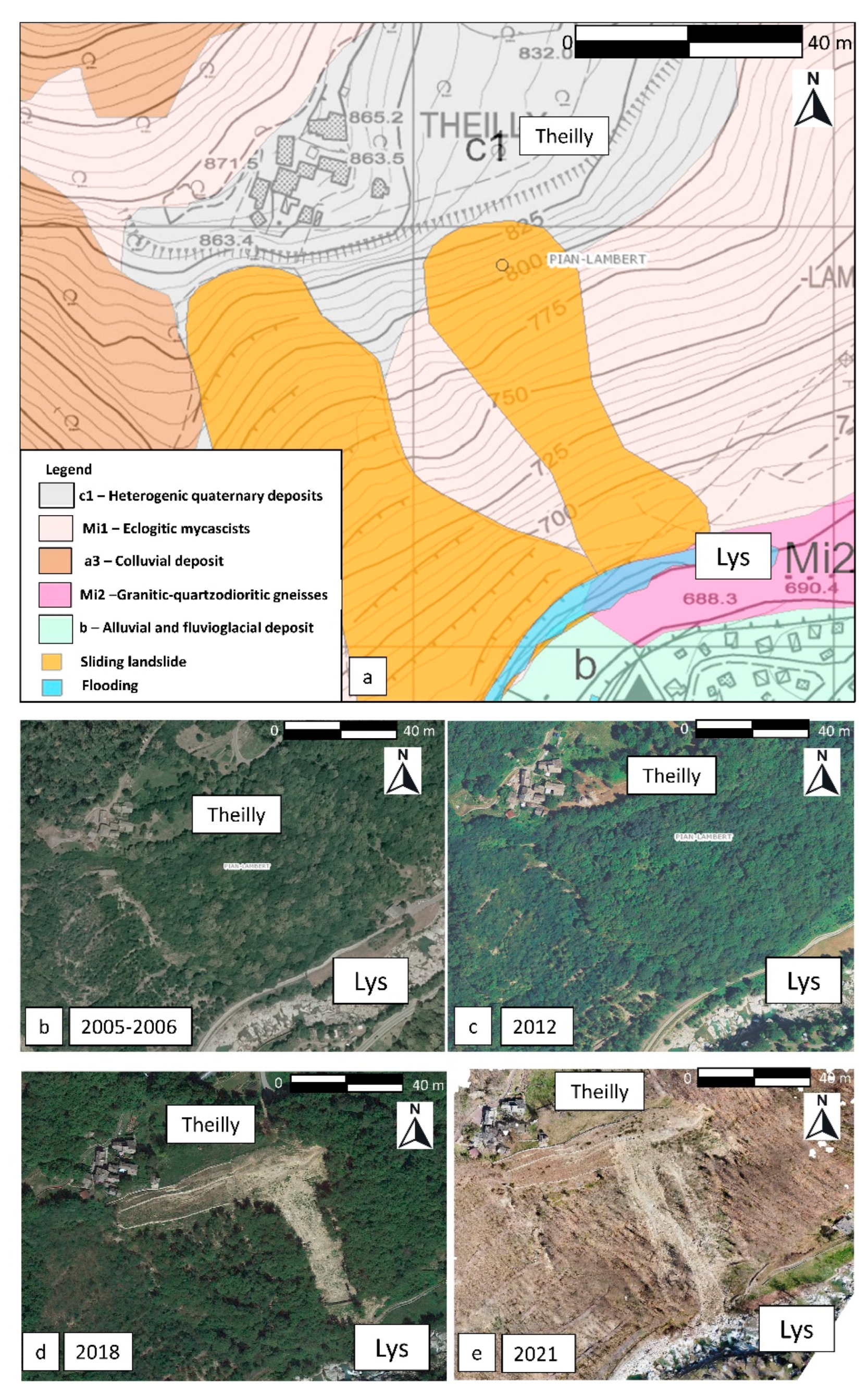
2. Study Area and Landslide Description

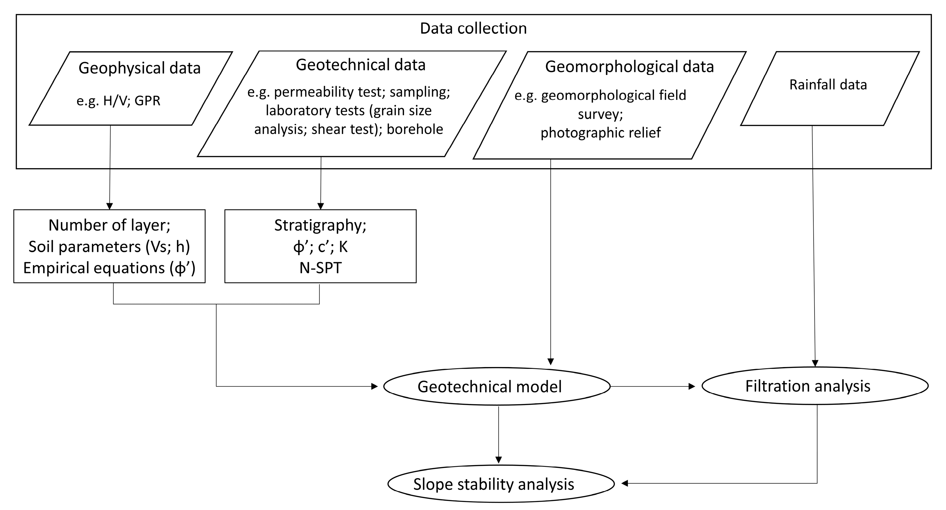
The village of Theilly (in the Fontainemore municipality, Aosta province, North-West Italy, Figure 1) rises at 840 m a.s.l. on the right bank of the Lys Stream. The slopes of the Lys valley were deeply modelled by the action of the great Quaternary glaciers and, subsequently, the valley was further eroded by four main processes: (a) the powerful action of the Lys stream, which engraved a V-shaped valley in the U-shaped glacial valley; (b) the erosive processes implemented by the surface and subsurface circulation of water; (c) the effect of gravity; and (d) the anthropic intervention. Therefore, the morphology of the area is typically post-glacial, characterised by the presence of the confluence step and the slope sector downstream of the main glacial terraces. In particular, the steep slope of Theilly is made up of a thick Quaternary detrital cover characterised by detrital deposits of mixed genesis (deposits consisting of materials linked to the rehash of pre-existing deposits, mainly glacial deposits), and undifferentiated glacial deposits (heterogeneous deposits, made up of blocks of various kinds immersed in a silty–sandy matrix [45] (Figure 1a). This interpretation is based on direct evidence gathered during a dedicated geological survey [46] and is consistent with the information on regional geological maps at a scale of 1:100,000. The blocks have dimensions from centimeters to meters. The rocky substratum is mainly made up of micaschists. The slopes of the Lys valley are also characterised by important water circulation, and, thanks to the high permeability of the deposits and the fractures of the bedrock, the water quickly reaches the valley, where the rocky substrate emerges.

The Theilly landslide is classified as a shallow slide [5] affecting the debris deposits on the slope downstream of the Theilly village. The sliding of the moraine material, arranged on very high slopes, was caused by the undermining of the foot by the Lys stream. Disasters in this sector have been ongoing for a long time, but the first reports recorded date back to 1975. Since 2011, numerous interventions have been carried out to restore and safeguard the village, through the installation of gabions, which have allowed the revegetation of a large part of the affected area (Figure 1b–e), without however resolving the instability situation. Despite the restoration work, the landslide under study underwent several reactivations, with damage to the gabions and falling blocks. Three major reactivations are highlighted: 25–28 November 2016, 24 November 2019 and 2–3 October 2020. All reactivations of the landslide occurred following heavy rainfall of short duration, without however resolving the situation of instability.

3. Methods

The main goals of the work were the evaluation of the stability of the Theilly landslide and the assessment of the triggering mechanism. The workflow is characterised by two main phases:

• processing and integration of geological, geophysical and spatial data;
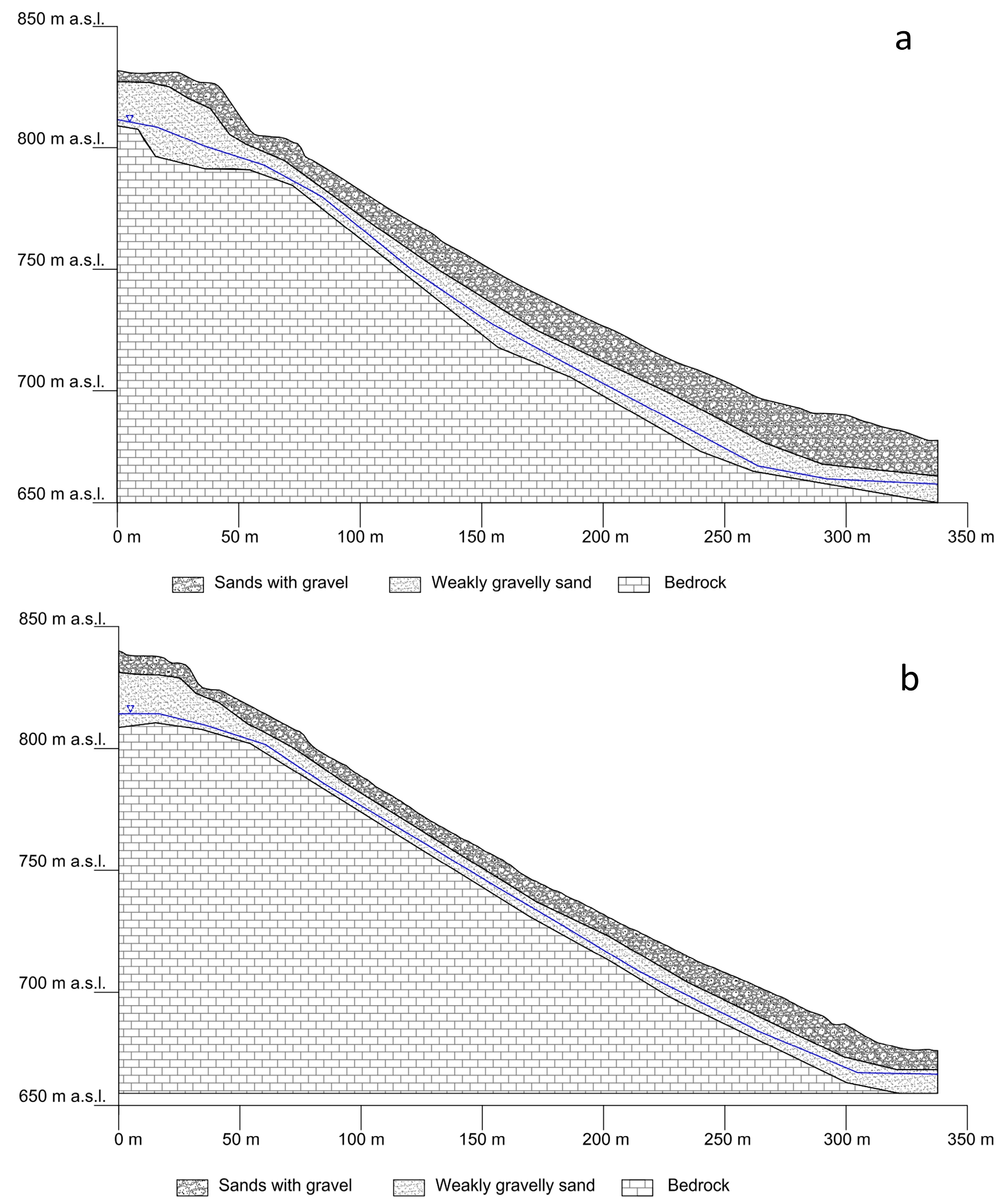
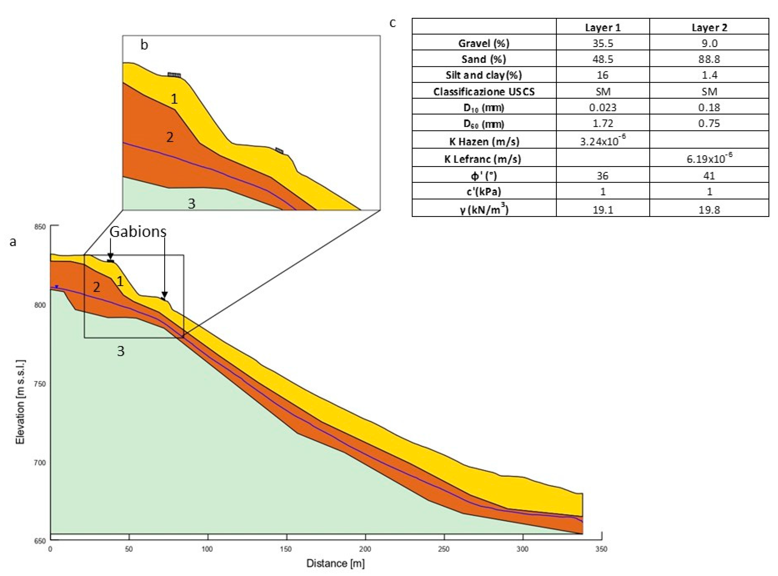
• stability analysis of two representative sections of the geotechnical model (Figure 2).

The geological model of the slope was created integrating geophysical and geotechnical data collected in two campaigns (September–October 2021). All the available data were used to build the geotechnical model of the slope in terms of stratigraphy, slope geometry and geotechnical parameters for slope stability analysis through hydrological–geotechnical modelling.

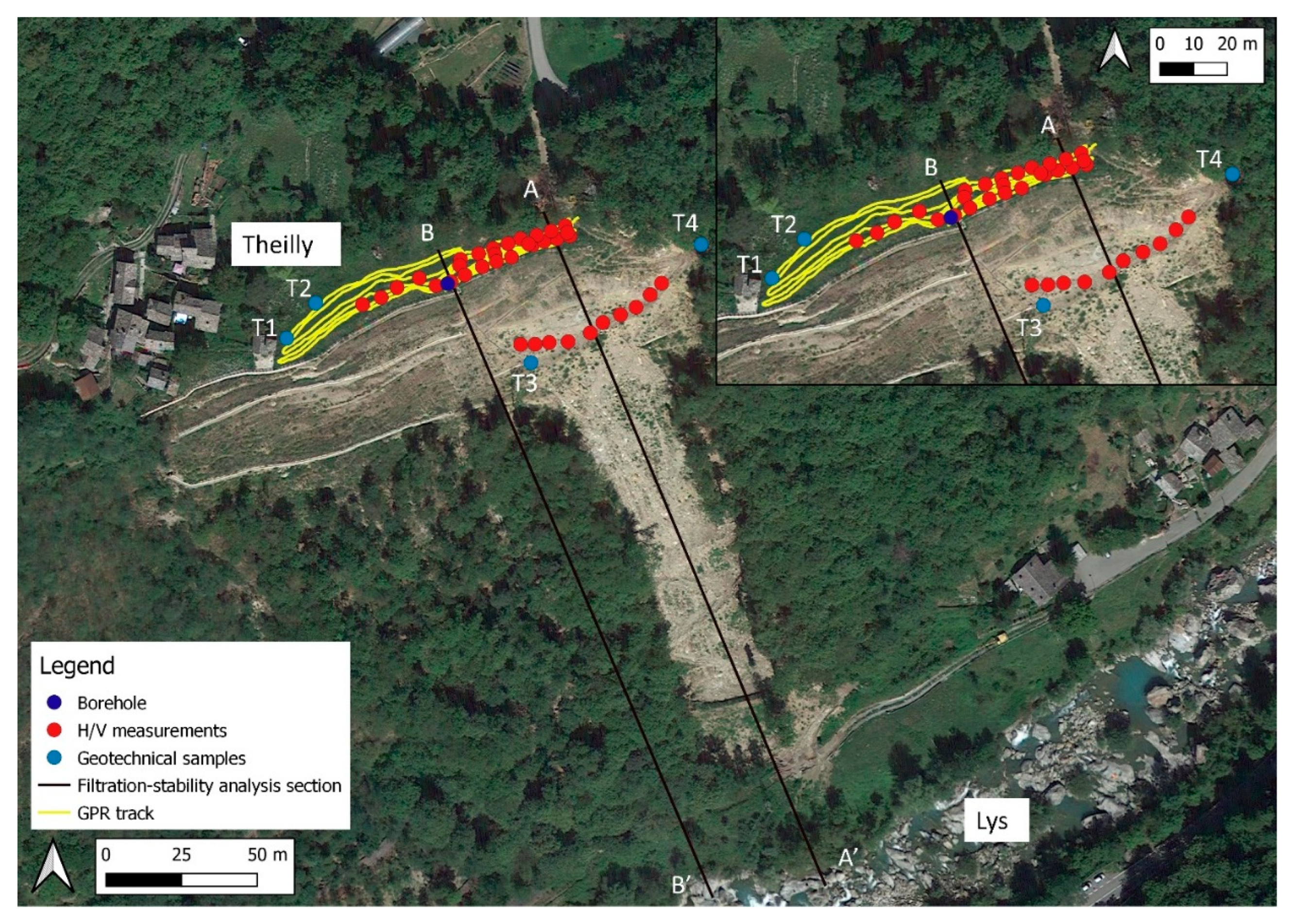
3.1. Geophysical Survey

Geophysical investigations (seismic noise single-station measures and GPR) were conducted with the aim of characterising the landslide slope to identify the layering and potential slip surface. Given the characteristics of the slope and the fact that the landslide area was difficult to access to instrumentation, 35 single-station passive seismic (H/V) measurements (red dots in Figure 3) were carried out and paired with a ground penetrating radar (GPR) survey (yellow lines in Figure 3) on the terrace above the slope (Figure 3).

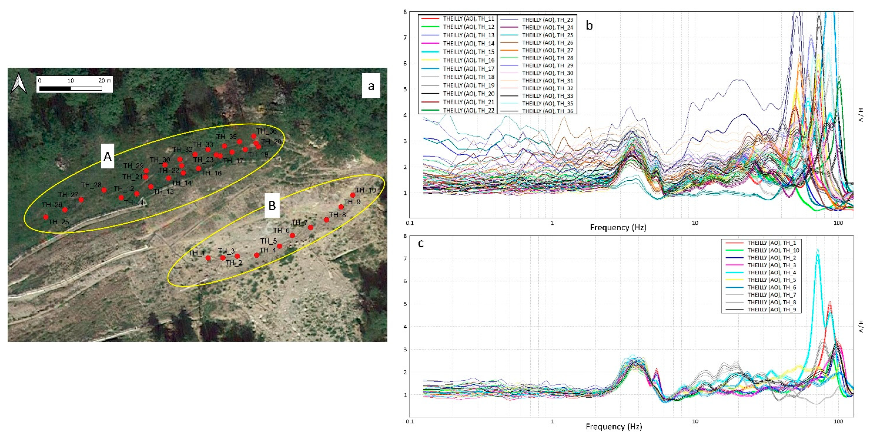
3.1.1. H/V Measurements

The microtremor methodology is a passive single-station analysis technique of environmental seismic noise. The term microtremor refers to all surface vibrations, characterised by low energy levels and low amplitudes, generated by both natural and anthropogenic sources [48]. The horizontal-to-vertical spectral ratio (HVSR or H/V) technique developed by [26] allows the natural frequency of vibration of a sedimentary deposit to be determined. The spectral relationship between the amplitude of the microtremor measured along the horizontal components (H) and the vertical ones (V) is assessed, as it is strongly correlated with the geological setting of the site (e.g., [22,49,50]. The HVSR technique therefore allows the fundamental or resonance frequency of a soil to be determined. The H/V ratio curve shows the presence of one or more frequency peak/s in the case of heterogeneous soils with high acoustic impedance contrasts. The peaks correspond to the presence of several layers with different lithology and depth. If the depth (z) or S-wave velocity (V_S) of the upper layer is known, it is then possible to reconstruct the V_S–z profile of the subsoil [51] according to the well-known law:

$$\mathrm{f}=\frac{{\mathrm{V}}_{\mathrm{S}}}{4·\mathrm{h}}$$

(1)

where h indicates the thickness of the layer. For this purpose, 35 H/V measurements were collected near the landslide crown and within the landslide body (green dots in Figure 3). The measurements were carried out using four three-way digital tromometers. Measurements were carried out under free field conditions, setting a sampling frequency of 256 Hz and an acquisition time length of 20 min. The acquired measurements were analysed and processed using the Grilla^® software, and all records were processed in the frequency range 0–128 Hz, considering time windows of 20 s each and applying a smoothing technique based on a triangular window with an amplitude of 10%.

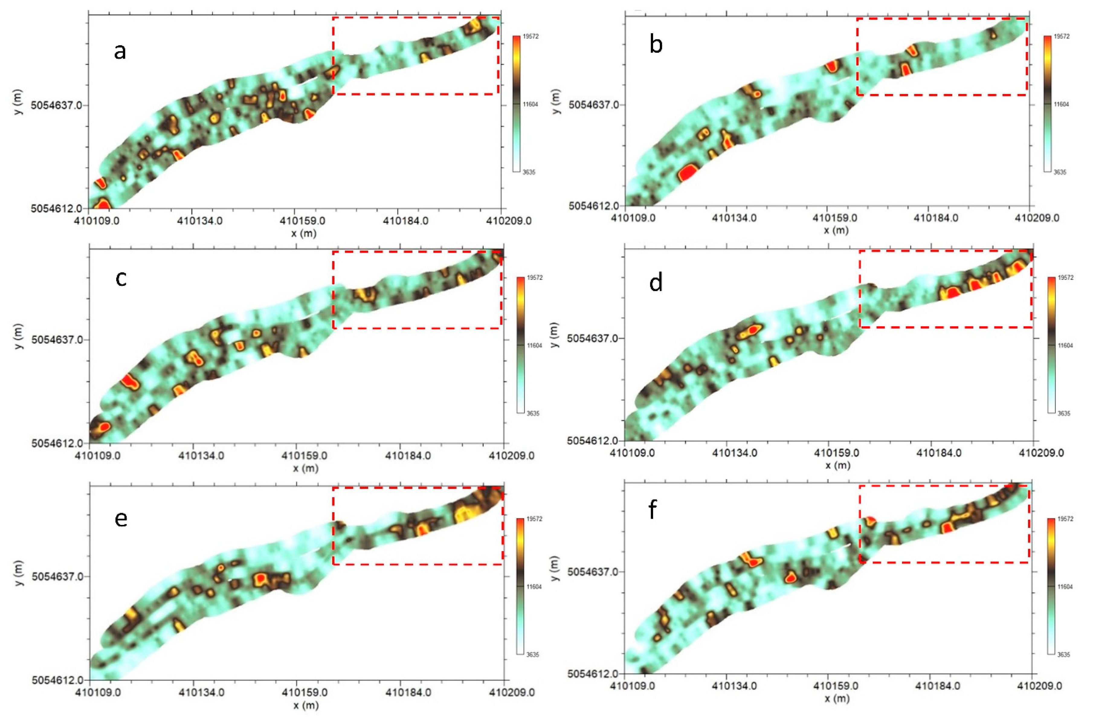
3.1.2. GPR Measurements

The GPR technique is a geophysical, non-invasive and non-destructive method that has become widely established in recent years due to its ability to return high-resolution images of the area under investigation [33,38]. GPR is widely used in the fields of geology for the identification of cavities, piezometric surface, stratigraphic succession and location of buried services [18,24,37,38,52,53,54,55,56], and archaeology [57] and engineering [58,59,60].

The GPR method identifies changes in the physical properties of soil using an electromagnetic pulse generated by a radar antenna ([61,62,63,64] and references within). The electromagnetic wave emitted by the transmitting antenna propagates in the subsurface at a speed dictated by the dielectric characteristics of the materials. The emitted pulse is reflected by the discontinuities/interfaces present in the subsoil or by the objects having different relative dielectric permittivity, and then it is recorded by the receiving antenna that measures the travel time [38,65,66]. The GPR method can reconstruct the stratigraphic and hydrogeological characteristics of the subsurface.

The GPR instrument used in this study is the Cobra CBD Radarteam Sweden antenna; it is a triple-band antenna with a frequency of 200–800 MHz, having decimetre resolution. It is suitable for surveys with high resolution and limited depth of investigation. The depth of investigation is a function of the frequency of the antenna and the electrical conductivity of the soils being surveyed. In this specific case, profiles were performed on the terrace at the escarpment with the objective of extracting information on the shallow stratigraphy (first 6 m), evidenced by previous site restoration work. Yellow lines in Figure 3 show the GPR traces performed.

3.2. Empirical Equations and N-SPT

An efficient stability analysis is closely related to a good assignment of geotechnical parameters (φ′ and c′) to the strata identified in the construction of the geological model. However, it is not always possible to determine the geotechnical parameters from direct tests, but indirect methods exist in the literature to be able to trace the values of φ′ and c′ also by using seismic parameters (V_S) [67,68].

Shear wave velocity (V_S) is a fundamental parameter for studying the dynamic properties of soils. Numerous empirical correlations exist in the literature that relate the value of Vs to in situ tests such as the SPT test. In the absence of the direct measurements of Vs or N-SPT, one of these values can be determined by indirect methods. Since the 1970s, numerous Vs and N-SPT correlation studies have been conducted in Japan and the United States, among which it is necessary to mention: [69,70,71,72,73,74,75,76]. There is extensive literature on these correlations, the different fields of application [77,78,79,80,81,82,83,84] and their use for all soil types [85,86,87].

Most of the correlations in the literature have the following form:

$${\mathrm{V}}_{\mathrm{S}}=\mathrm{a}·{\left({\mathrm{N}}_{\mathrm{S}\mathrm{P}\mathrm{T}}\right)}^{\mathrm{b}}$$

(2)

where the constants a and b were determined by different authors from a data set and by statistical regressions. Therefore, by knowing the value of Vs or N-SPT, it is possible to trace back by direct or inverse formula to one of the two unknowns.

Moreover, by having the value of N-SPT, it is possible to derive the value of the friction angle φ′ directly using the RBS (road bridge specification) direct correlation method, which is based on the following relationship:

$$\mathsf{\phi }\prime =\sqrt{15·{\mathrm{N}}_{\mathrm{N}\mathrm{O}\mathrm{R}\mathrm{M}}}+15$$

(3)

where N_NORM denotes the normalised value, derived from the following correlation:

$${\mathrm{N}}_{\mathrm{N}\mathrm{O}\mathrm{R}\mathrm{M}}={\left(\frac{{\mathsf{\sigma }}_0^{\prime }}{{\mathsf{\sigma }}_{\mathrm{v}0}^{\prime }}\right)}^{0.5}·{\mathrm{N}}_{\mathrm{S}\mathrm{P}\mathrm{T}}$$

(4)

where σ′₀ is the reference lithostatic pressure, assumed to be 100 kPa, and σ′_v0 is the effective vertical pressure at the depth of the test.

In this study, the Equations (2)–(4) were used to determine the value of N-SPT from the known V_S, expressing N-SPT as:

$${\mathrm{N}}_{\mathrm{S}\mathrm{P}\mathrm{T}}={\left(\frac{{\mathrm{V}}_{\mathrm{S}}}{\mathrm{a}}\right)}^{\frac{1}{\mathrm{b}}}$$

(5)

The SPT test is among the most widely used methods for obtaining information on poorly cohesive soils. This test returns with good reliability the properties of the investigated soils, such as φ′, relative density (Dr), Young’s elastic modulus and S-wave velocity (V_S) [8,8]. By knowing the number of N-SPT blows from direct in situ measurements, it is possible to obtain φ′ through correlations found in the literature.

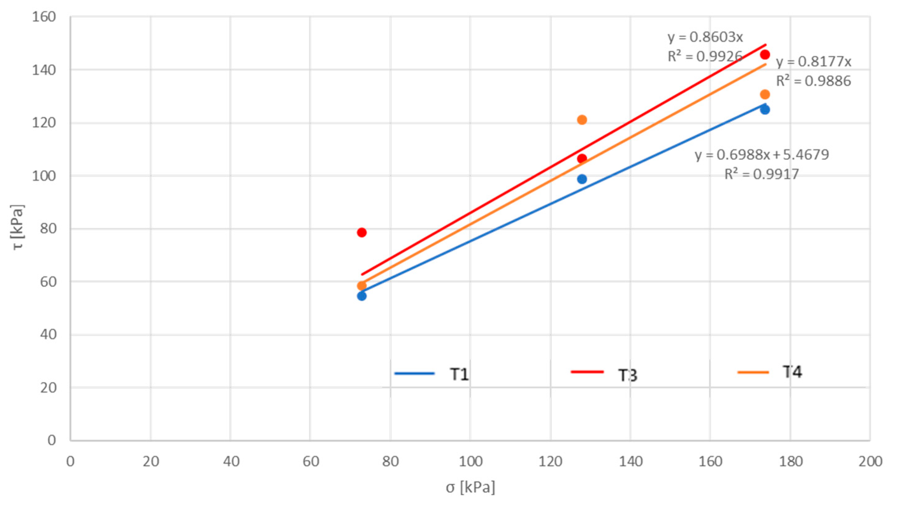
3.3. Geotechnical Surveys

Geotechnical characterisation of the materials affected by the landslide was carried out through laboratory tests and geognostic survey. The laboratory tests, performed on samples collected in situ, consisted of (i) grain size analysis, (ii) determination of index properties and (iii) determination of shear strength parameters. Blue dots in Figure 3 show the location of the sampling sites: samples were collected at different locations on the slope (both inside and outside the landslide body), at different depths (0.25 m, 0.37 m and 0.20 m), to characterise in detail the materials involved in the slope dynamics.

Particle size analysis of the samples was performed by wet sieving in accordance with ASTM (American Society for Testing and Materials) international standards [88]. The evaluation of the saturated hydraulic conductivity (K_sat) was performed in situ using a portable constant-load permeability measuring device (Amoozmeter or CCHP, Compact Constant Head Permeameter, [89]). Due to the nature of the soil, only one in situ saturated permeability test could be performed at the T2 sampling point (Figure 3), at a depth of 37 cm from ground level. The results were interpreted according to Glover’s solution [90,91,92]. Shear strength parameters (effective friction angle φ′ and effective cohesion c′) of the samples were determined by means of consolidated and drained direct shear tests under saturated conditions with Casagrande-type shear equipment, applying procedures standardized by [93]. Shear stages on the investigated samples were carried out using normal load values (σ_N) of 73 kPa, 128 kPa and 177 kPa. The results are compatible with the data set of data present in [94] and relating to similar terrains.

In addition, the geotechnical investigations included the drilling of a geognostic borehole for continuous core investigation near the escarpment (yellow dot in Figure 3). The investigation was conducted with the aim of determining the lithological and geotechnical characteristics of the soils involved in the movement. The survey performed by continuous coring reached a depth of 40 m and was equipped with an open-tube piezometer. During the execution of the survey, 9 SPTs (standard penetration tests) were performed at the following depths: 3.0 m; 6.0 m; 9.0 m; 12.0 m; 18.0 m; 21.0 m; 24.0 m; 27.0 m and 33.0 m. The SPT [95] measures the number (N) of blows required to infill a standard mallet percussively, with a predetermined drop height, a standard sampler. The sampler is lowered into the borehole until it rests on the level to be examined. The number of blows required to penetrate it by 30 cm is called the number of blows N-SPT [25]. In addition, 7 soil samples were collected, on which grain size analysis was performed. Finally, 4 Lefranc permeability tests were performed [96]. The results of geotechnical investigations are reported in Section 4.2.

3.4. Slope Stability

The analysis of the triggering conditions of the Theilly landslide was conducted by hydrological and geotechnical modelling, which allowed the identification of the variation of the FS in response to various rainfall events. Combined filtration–stability analysis was conducted with the codes SEEP/W and SLOPE/W, both belonging to the GeoStudio 2020 package [39,40].

Slope modelling in response to the rainfall event, i.e., analysis of saturated and unsaturated flow along the slope under transient conditions, was conducted with the finite element code SEEP/W. The code is based on the filtration law formulated by [97], which describes the motion of water in a saturated soil. The law was later modified by extending it to unsaturated soils [98,99]. The filtration model adopted is based on the equation of motion and the equation of conservation of mass, in the form extended to unsaturated conditions [99,100]. Under transient conditions, the input data are the precipitation values along the entire surface of the section under analysis. The filtration analysis made it possible to reconstruct, in the slope affected by the landslide, the trend of interstitial soil pressures as a function of the rainfall regime for the thirty days preceding the event.

The stability analysis was performed with SLOPE/W software. The negative and positive interstitial pressure distributions calculated with the SEEP/W model during the events were incorporated within the stability analysis. The code implemented the limit equilibrium method (LEM), and the slope FS was calculated using the method of [41], in which the relationship between vertical and horizontal interface forces is expressed through an unknown function in which the parameters are derived from the global mass balance ([13] and references therein). The code usesof the Mohr–Coulomb criterion in terms of effective stresses in the case of positive interstitial pressures, and the equation of [101] in the case of negative interstitial pressures. In particular, the equation of [101] allows the quantification of material strength under undersaturated conditions through the material characteristic curve and effective shear strength parameters.

4. Results

4.1. Geophysical Results

The distribution of single-station seismic noise measurements is shown in Figure 4a. The 35 H/V measurements have been grouped into two sets (A and B in Figure 4a). Figure 4b shows the H/V curves of group A, recorded near the landslide crown, while Figure 4c shows the curves of group B, recorded on the landslide body. Thanks to previous studies conducted on the landslide, it was possible to constrain by means of the Vs (

Table 1. Values of f (frequency), depth (h) and mean S-wave velocity (Vs) for each of the each of the seismo-layers identified by the HVSR analysis.

Seismo-Layer	f (Hz)	h (m)	Vs (m/s)
1	20–35	2–4	298
2	3.3–4.3	18–35	433
3	/	∞	832

) the main identified natural peaks and determine the layer depth by solving Equation (1). Both sections show the presence of a natural peak at about 3.3–4.3 Hz, corresponding to a depth of about 18–35 m. It can be attributed to the interface between the weathered material and the unweathered substratum. Some of the peaks at higher frequencies are both natural and anthropogenic peaks. In particular, the presence of a second natural peak (group B) at high frequencies of approximately 20–35 Hz, corresponding to a depth of 2–4 m, is evident. It can be attributed to the interface between the anthropogenic fill present in the area and the landslide.

The acquired GPR data made it possible to create representative subsurface sections at different depths (Figure 5) of the investigated area. The colour scale represents the medium’s ability to absorb the impulse (cold colours) or reflect the signal (warm colours). Therefore, a homogeneous and uniform medium will allow the signal to pass through undisturbed, resulting in cold tones, while an anisotropic medium will show warmer colours. The rectangle in red in Figure 5 shows the area affected by the landslide. At depths between 1 and 4 m, there is an increase in interference, probably produced by the chaotic material in situ. In this area, the investigation went down to a depth of 6 m, allowing a detailed study of the area close to the crown of the landslide, where anthropogenic filling had taken place because of the slope restoration work (approximately 4 m thick). Starting from a depth of 4 m, in the red rectangle, the presence of an anomaly (warm colours) extending up to 6 m (maximum depth reached by the survey) is noted. This anomaly can be traced back to a stratigraphic change associated with the presence of decimetric-sized gneiss blocks in this area. The investigation allowed for an understanding of the thickness and extent of the fill, highlighting portions of major anomalies at different depths associated with gneiss blocks of different sizes and the presence of an extremely heterogeneous layer 5–6 m thick.

4.2. Geotechnical Results

The samples analysed are representative of soils characterised by heterogeneous grain size. They are mainly granular soils, with a predominance of a sandy fraction in samples T1, T2 and T3, and a predominance of a gravelly fraction in sample T4. Based on grain size analysis results, the soils involved in the landslide movement are classifiable as silty sands (SM) according to USCS (Unified Soil Classification System) classification. Data from direct shear tests indicated friction angle values in the range of 35° to 39.4° and a cohesion of 5.5 kPa (Figure 6).

Table 2. Summary of the geotechnical parameters of the four samples collected from the Theilly landslide. K = permeability constant load test; w = water content; φ′ = friction angle; and c′ = cohesion.

Sample	T1	T2	T3	T4
Depth (m)	0.25	0.37	0.2	0.25
Gravel (%)	31.2	20.7	35.5	41.8
Sand (%)	36.8	40.2	48.5	34.1
Silt (%)	30.4	39	16	23.4
Clay (%)	1.6	0.1	/	0.7
USCS Classification	SM	SM	SM	SM
K (m/sec)	/	8.87 × 10−6	/	/
K Hazen (m/s)	2.56 × 10−6	9.02 × 10−7	/	3.24 × 10−6
w (%)	8.6	33	1	2.8
φ′ (°)	35	/	39.4	38.4
c′ (kPa)	5.5	/	0	0

shows the results of the tests performed on the samples.

The stratigraphy derived from the borehole showed the presence of reworked soil, classified as anthropogenic fill, up to a depth of 7.5 m. From that depth, the survey showed an alternation of coarse gravel with a sandy matrix that was partially-to-well cemented and medium-to-coarse sand with pebbles of varying sizes, from millimetres to centimetres. These gravel and sand layers were interrupted in the sequence by the presence of leucocratic gneiss blocks with quartz, white mica, k-feldspar and chlorite. The results of particle size analysis and the Lefranc permeability test, performed on the seven samples taken during the survey, are summarised in

Table 3. Summary of the geotechnical parameters of the borehole. C1, C2, C3 and C4 indicate the samples at various depths on which the tests were performed. K = permeability coefficient determined by the Lefranc permeability test.

Sample	C1	C2	C3	C4	C5	C6	C7
Depth (m)	4.5–4.8	10.0–10.2	14.5–14.7	18.20–18.50	20.0–20.40	30.0–30.3	33.3–33.6
Pebble (%)	19.4	31.5	/	/	/	/	/
Gravel (%)	35.2	30.1	9.8	52.2	34.4	47.2	23.9
Sand (%)	30.6	23.3	88.8	36.4	49.1	32.8	62.3
Silt/Clay (%)	14.8	15.1	1.4	11.4	15.5	18.8	13.8
USCS Classification	GM-GC	GM-GC	SW	GW-GM	SM-SC	SM-SC	SM-SC
K (m/s)	/	6.9 × 10−6	/	/	2.14 × 10−5	4.94 × 10−6	1.08 × 10−5

.

Figure 7 shows the geological sections along the two investigated profiles, created using the data derived from the stratigraphic survey and laboratory tests performed on the samples taken.

Of the nine SPT tests performed, only those at a depth of 12.45 m (N-SPT = 44) and at 21.45 m (N-SPT = 80) were usable. The remaining seven failed, as the number of hits (N) exceeded the value of 50 for a 15 cm section, this value representing ‘Rejection’, i.e., the end of the test.

4.3. Landslide Modelling

The geophysical investigations, the geotechnical characterisation of materials in situ and in the laboratory, and the results of the survey allowed the creation of a detailed geotechnical model of the landslide area. The data agreed in showing the presence of three layers, characterised by an increase in the degree of thickening with depth. It is justified by an increase in seismic wave velocities and by an alternation of coarse sands and gravels with a sandy matrix, whose cementation increases with depth, interspersed with altered gneissic blocks. Slope modelling was carried out in two areas of the slope by making two geological–technical sections (A–A’ and B–B’) (black lines in Figure 3). Section A–A’ covers the slope section affected by the 2020 landslide. Section B–B’, on the other hand, covers a portion upstream of the landslide at the point where the geognostic survey was performed. For each of the two sections, two topographic profiles were obtained from the digital terrain model (DTM) data with 1 m resolution, made available by the Valle d’Aosta Region.

The geotechnical model of the slope can be simplified, proceeding from ground level to depth, with the following three layers. Layer 1—surface detritus consisting mainly of sands with gravel varying in thickness from 3 m (at the landslide crown) to 15 m along the landslide body. Layer 2—weakly thickened slope deposits. This is an underlying layer of increasingly thickened materials consisting mainly of weakly gravelly sand. The thickness of this layer varies between 5 and 15 m. Layer 3—the bedrock. Considering the nature of the landslide and its characteristics, the search for critical surfaces was only conducted in the first two layers, as the substrate was never affected by movements during landslide reactivations. The geotechnical and hydrological parameters of the first two levels were obtained by combining all the analyses conducted and described in the previous paragraphs. Table 1 shows the values assigned to the two modelled layers. The bedrock parameters have not been reported as it was considered impenetrable. The water table level for the two sections was defined based on the depth found during the survey and is located for both sections within Layer 2.

The modelling made it possible to define the behaviour of the slope under various rainfall scenarios without and with the stabilisation measures carried out in 2011. In particular, the filtration–stability conditions were evaluated for three main rainfall events (see [45]) that produced a reactivation of the landslide: 25–28 November 2016; 24 November 2019 and 2–3 October 2020 (Figure 8). Finally, a model of filtration stability was analysed, considering the effect of vegetation in terms of increased root cohesion.

To simulate the stabilisation interventions, a vertical overload corresponding to the weight of these gabions, estimated from technical data in the literature, was applied (Figure 9).

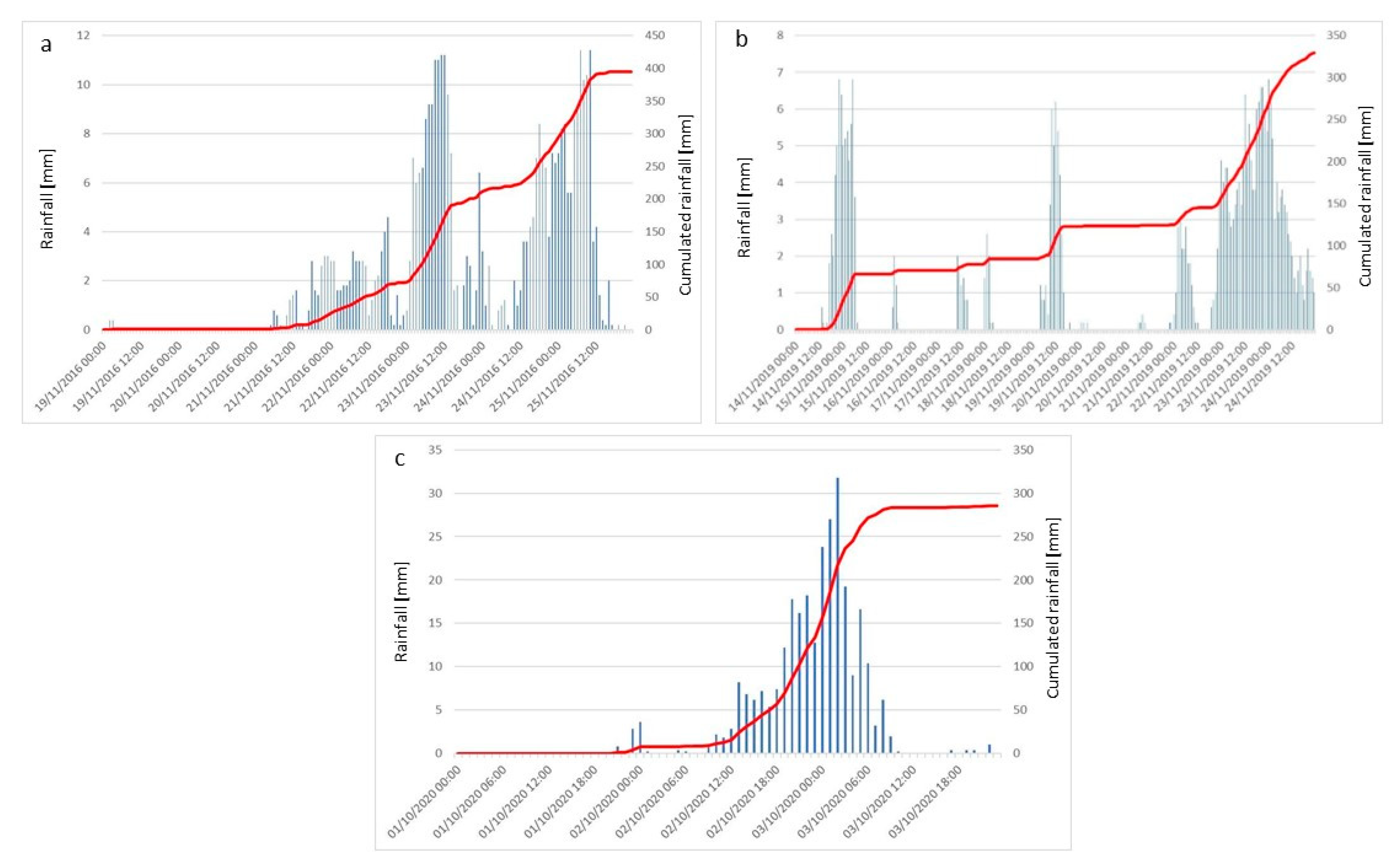
4.4. Filtration Analysis

The filtration analysis, conducted on Sections A–A’ and B–B’ for all three events (2016, 2019 and 2020), allowed us to reconstruct the slope’s filtration mechanism considering the precipitation in the thirty days before the event (only one day’s analysis is shown here; for the remainder see the Supplementary Materials section). The analysis showed for all events a top-down saturation mechanism.

Section A–A’

The 25–28 November 2016 rainfall event was characterised by high intensity and short duration. Figure 10a shows the interstitial pressures for 26 November 2016, obtained using the SEEP/W software. Initially (20 November), Layer 1 was in an undersaturated condition; with the onset of precipitation on 21 November, the interstitial pressures of the more superficial horizons began to increase, taking on positive values and reaching maximum values (around 2 kPa) from 24 November. Figure 10a shows the water pressure profiles within the layer for a depth of about 10 m. The deep portion of Layer 1 was not affected by pressure variations, in accordance with the dynamics of the rainfall event, characterised by a short duration and high intensity of precipitation, which partly led to the saturation of the first soil layers and partly flowed down the slope, also due to the latter’s high acclivity.

The November 2019 rainfall event had a longer duration than that of 2016 and was characterised by several intervals of short duration and high intensity that led to the progressive saturation of the soil horizons of Layer 1. Figure 10b shows the changes in interstitial pressures along the slope, while the graph shows the water pressure profiles within Layer 1 for a depth of approximately 7 m. The analysis determines an initial undersaturation of Layer 1. The rainfall events recorded between 13 and 15 November saturated the more superficial soil layers, generating slightly positive interstitial pressures. Subsequent rainfall events contributed to the maintenance of saturation and allowed the infiltration of water into the lower layers and the consequent increase in interstitial pressures, until the rainfall event that began on 22 November produced an increase in interstitial pressures, destabilising the slope. The change in pressures was therefore consistent with the dynamics of the rainfall event characterised by relatively heavy rainfall, which led to the saturation of soil Layer 1. The 22–24 November event, characterised by high intensity, led to the formation of overpressures in the most superficial layers.

The October 2020 rainfall event was characterised by a short duration and very high rainfall intensity, with peaks of over 30 mm/h. This event led to a rapid saturation of the ground surface levels. The modelling was carried out by modifying the topographic profile based on the in situ surveys and available photographic material, thus considering the effects of the 2016 and 2019 landslides, and eliminating the second order of works. Figure 10c shows the variation of interstitial pressures along the slope, while the graph shows the water pressure profiles within Layer 1 for a depth of approximately 9 m. From the analysis, Layer 1 was in an undersaturated condition at the beginning of the rainfall event; with the rainfall recorded from 1 October onwards, the uppermost layer of the soil began to saturate, where positive interstitial pressures were generated. As the event continued, the lower levels also began to saturate. This behaviour is consistent with the dynamics of the rainfall event, the short duration of which, combined with a very high rainfall intensity, exceeded the infiltration capacity of the soil; this, in combination with the high slope gradient, resulted in the soil remaining undersaturated at depth.

Section B–B’

The filtration analysis along the B–B’ profile of the 25–28 November 2016 event showed a pressure distribution (Figure 11a) like that described for the A–A’ profile. At the beginning of the rainfall event, Layer 1 was undersaturated and, as the rainfall event progresses, a saturation phase of the more superficial soil layers began for a thickness of about 3 m.

The filtration analysis of the 24 November 2019 event confirmed the same saturation process that occurred in the A–A’ profile. Figure 11b shows the distribution of interstitial pressures, while the graph (Figure 11b) illustrates the water pressure profiles within Layer 1. The water was initially undersaturated, then began to saturate in the more superficial layers with the onset of precipitation. As precipitation continued, characterised by several medium-intensity events, the slope became progressively saturated down to a depth of approximately 8 m.

The filtration analysis of the last event (2–3 October 2020) on this portion of the slope confirms what was observed for section A–A’; in this case too, it can be observed that layer 1 was initially undersaturated (Figure 11c), then with the onset of rainfall the saturation of the more superficial soil levels was observed (graph Figure 11c), to a thickness of about 1 m, while at greater depths no overpressure formation was observed. Again, the distribution of interstitial pressures and their temporal evolution were consistent with the dynamics of an extremely intense and brief rainfall event, which at times exceeded the infiltration capacity of the soil.

4.5. Stability Analysis

The stability analysis was carried out for each event (2016, 2019 and 2020) evaluating for section A–A’ the FS both in the presence and absence of the structural works (gabion wall); meanwhile the collapse of the gabions at the section had occurred, and it was necessary to evaluate the FS both in the presence and absence of the works. Meanwhile, for section B–B’, the analysis was conducted only in the presence of gabion walls, since the collapse of the gabions did not occur in this area and looking for the critical surface in the slope section that included the order of gabion walls downstream of the slope, so that the results could be compared with section A–A’.

The modelling carried out along section A–A’ and relating to the event of 24–26 November 2016 (Figure 12) showed, in the presence of gabion walls, the development of the most critical slip surface upstream of the second order of gabion walls propagating downstream for 40 m. The analysis of the FS showed a slope in a precarious condition already at the beginning of the rainfall event (FS = 1.1) and which, as the rainfall progressed, reached borderline equilibrium conditions between 23 and 24 November (FS = 1.05), when the landslide occurred (Figure 13). The same section in the absence of gabion walls showed a sliding surface like the modelling in the presence of structural works and originating at the same point (Figure 12). Similarly, the evolution of the FS during the rainfall event showed a similar trend; however, the FS values were slightly higher, since at the beginning of the event FS = 1.15, which then decreased to a value of 1.08 between 24 and 25 November (Figure 13).

On the other hand, the modelling carried out along section B–B’ for the 2016 event identified the most critical surface downstream of the last order of gabion walls (Figure 12), with the development of a surface landslide of approximately 50 m in length. The evolution of the factor of safety during the rain event showed that the slope was in a precarious equilibrium condition, with a minimum FS value of 1.09 and a maximum of 1.15 (Figure 13).

The stability analysis of the 24 November 2019 event was performed with the same settings as the modelling of the 2016 event, as no information on the geometry of the landslide generated was available. The simulation along section A–A’ (Figure 12) in the presence of gabion walls developed, as in the previous case, downstream of the second order of gabion walls. The FS at the beginning of the event presented a value of 1.12, which decreased to 1.03 as the rainfall event progressed (Figure 13). In the absence of gabions, the critical surface identified was almost identical to the surface in the presence of gabions. Similarly, the FS presented an evolution very similar to that in the presence of works; however, the minimum value stopped at 1.06. Modelling along section B–B’ (Figure 12) identified the development of the most critical slip surface approximately 16 m downstream of the last order of gabion walls, with the creation of a surface landslide approximately 37 m long. The analysis of the FS highlighted the precarious balance of the slope; in fact, at the beginning of the rainfall event there were FS values of just over 1.1 (Figure 13), which decreased to values of just under 1.08 as the rainfall event continued.

The modelling of the event of 2–3 October 2020 identified along section A–A’ in the presence of the works (Figure 12) a sliding surface with an extremely shallow depth (minimum thickness of 0.5 m and maximum within 2.5 m), which affected a part of the slope where the containment works were located. The analysis of the factor of safety (Figure 13) showed a condition of boundary equilibrium of this portion of the slope already with the onset of rain (FS = 1.0); however, with the evolution of the meteorological event, the FS did not vary.

The simulation conducted in the absence of overburden (Figure 12) revealed, during the October 2020 event, a critical sliding surface almost coinciding in location and size with that identified by simulating the presence of overburden. The evolution of the FS (Figure 13) also showed a similar trend to that seen previously, although with slightly higher FS values, reaching a minimum value of 1.03.

The stability analysis along section B–B’ (Figure 12) showed that on this portion of the slope the most critical surface was generated approximately 12 m downstream of the last order of gabion walls, with the creation of a surface landslide approximately 37 m long. The analysis of the FS, also in this case, highlighted the precarious equilibrium of the slope; in fact, at the beginning of the rainfall event, FS values of slightly more than 1.1 were recorded (Figure 13), consistent with the results of the simulations of the previous events. However, in this case, no reduction in the FS values was observed as the rainfall event evolved.

5. Discussion

The analysis of geophysical and geotechnical data combined with the support of spatial data (DTM) allowed the reconstruction of a detailed geological model of the Theilly landslide. The HVSR investigation led to the identification of two important natural peaks, one at high frequencies (20–35 Hz), which made it possible to identify the thickness of the material reworked by anthropic intervention, and one at low frequencies (3.3–4.3 Hz), attributable to a deeper level (20–30 m), characterised by a high Vs value (>800 m/s).

The geotechnical investigation confirmed the presence of a strong layer of reworked soil between 3 and 4 m thick, below which there was an alternation of coarse sands and gravels immersed in a sandy–loam matrix, interspersed with gneiss blocks. The geotechnical investigation associated with the geophysical investigation made it possible to reconstruct the geometry of the slope and its thicknesses and to derive the geotechnical parameters for the filtration–stability analysis.

5.1. V_S-N-SPT-φ′ Correlation and Evaluation

In Section 3.2, it is shown how the Vs values can be related to the N-SPT and, by having the value of N-SPT, how it is possible to derive the friction angle φ′ directly. As presented in the Results section, the H/V data made it possible to relate the depth of the interface to the frequency of the identified peaks and to the Vs of the identified seismo-layers. Thus, empirical equations could be applied to derive the value of N-SPT, and consequently φ′, from the Vs obtained by means of H/V measures. Of course, the estimation of N-SPT values from geophysical data is affected by a higher level of uncertainty, compared with the direct measure during a borehole survey. Nevertheless, this N-SPT indirect estimation could be very useful in the first phases of an emergency when direct data are not available, and a preliminary back and forward stability analysis could be performed to evaluate the landslide evolution and to assess civil protection actions. In the following, the goodness and reliability of this procedure is shown and discussed.

Table 4. Values of the coefficients a and b proposed by 17 different authors and used to estimate N-SPT. N_norm indicates the normalised value of NSPT and φ′ is the value of the friction angle obtained for each value of N-SPT.

			Seismo-Layer 1			Seismo-Layer 2
Authors	a	b	N-SPT	Nnorm	φ′	N-SPT	Nnorm	φ′
[71]	85.35	0.348	38	55	43	45	25	34
[102]	18.9	0.6	83	132	56	90	54	43
[103]	31.7	0.6	42	62	45	63	31	36
[104]	84	0.31	58	87	51	61	35	38
[105]	87.2	0.36	31	46	41	44	23	33
[70]	81.4	0.39	29	42	40	44	23	33
[70]	59.4	0.47	31	46	41	60	29	35
[72]	92	0.329	37	54	43	45	24	34
[106]	89.9	0.341	35	51	42	42	23	33
[107]	91	0.337	35	51	42	42	23	33
[108]	80	0.333	54	79	49	53	30	36
[109]	61	0.5	24	36	38	53	22	33
[110]	100.5	0.29	45	65	46	44	25	34
Muzzi (1984)1	80.6	0.331	54	79	49	53	30	36
[111]	65.58	0.502	21	30	36	45	19	32
[73]	157.4	0.49	29	43	40	61	28	35
[112]	104.7	0.296	36	53	43	35	20	32
Mean			40	59	44	52	27	35
Standard deviation			15.3	24.2	4.9	12.8	8.1	2.8

¹ Personal communication.

shows the values of coefficients a and b, proposed by 17 different authors and used in this work to estimate N-SPT. For the two main seismo-layers identified by the H/V measurements, the values of φ′ shown in Table 4 were determined, using the value of Vs employed in the H/V data and empirically deriving the value of N-SPT, which was necessary to determine the value of φ′.

Performing the survey and N-SPT tests made it possible to derive from direct formulas the value of φ′.

Table 5. φ′ values derived from the N-SPT value of the survey for each proposed author.

N-SPT from in situ Measurements	44	80
Depth (m)	85.35	0.348
Author	φ′
R.B.S	35.0	37.9
[113]	35.0	37.5
[114]	21.4	33.9
[70]	38.1	41.4
[115]	35.5	37.8
[116]	34.7	37.0
[117]	38.9	40.7
[118]	40.3	43.2
[119]	34.7	36.9
[120]	42.0	42.0

shows the calculated φ′ values for each of the correlations used. The N-SPT value of 44 (corresponding to the depth of 12.45 m) was used to calculate the φ′ value for Layer 1 and that of 80 (corresponding to the depth of 21.45 m) for Layer 2.

Comparing the φ′ values range obtained from the laboratory tests (35–39°), that of empirical V_S-N-SPT correlations (35–44°), and that from N-SPT correlations (36–39°), we observed that the φ′ value varied between a minimum value of 35° in all measurements and a maximum of 39° (laboratory tests and N-SPT correlation) and 44° (V_S-N-SPT correlation). The greatest variability, as expected, was observed in the φ′ value derived from the empirical correlations between Vs and N-SPT, while the laboratory and N-SPT data were very much in agreement in the value of φ′. However, a good agreement clearly emerged in the data obtained from direct and indirect measurements, making it reliable to estimate φ′ from geophysical data when direct N-SPT measures or soil samples are not available.

5.2. Effect of Vegetation on Slope Stability

The slope stability analysis for the 2016 event was repeated by inserting the effects of a possible grassing of the slope into the model. It is in fact known that the use of specific herbaceous species allows an increase in the stability of the slopes, increasing the cohesion of the soil (on average from 5 kPa to 8 kPa, [121]) and shear strength, but also reducing the infiltration of water and the superficial erosive processes [122]. To simulate this process, the geological model of the slope (limited to section A–A’) was modified, inserting a surface level with a thickness of 1 m, in which cohesion was increased to simulate the effect of the radical cohesion of the plants (Figure 14a). Cohesion was increased by 5 kPa, as indicated by the technical data of the literature. In addition, in this case, two simulations were carried out: with the gabions and without the gabions. For each of them, the most critical sliding surface identified previously was loaded (see Section 4.5) and the evolution of the FS was analysed. The evolution of the FS with the effect of radical cohesion, for the two scenarios, is shown Figure 14c, from which it is observed how the inclusion of an artificialised slope in the model allowed a significantly increase in the stability of the slope. In the presence of gabions, the FS values varied between 1.15 and 1.24, with a variable increase between 10 and 16% compared with the previous simulation. In the absence of gabions, the FS values varied between 1.16 and 1.24, with a variable increase between 7% and 10% compared with the previous simulation. In this simulation, the effect of reducing infiltration due to vegetation was not considered, and, consequently, the increases in the safety factor could be underestimated compared with the real ones.

6. Conclusions

Geophysical and geotechnical data combined with spatial data (DTM) allowed the reconstruction of a detailed geological–geotechnical model of the Theilly landslide. The SEEP/W simulations carried out for three selected rainfall events made it possible to reconstruct the dynamics of water filtration in the slope and the processes that led to the triggering of the landslide phenomena.

The results of the combined filtration–stability analysis showed that:

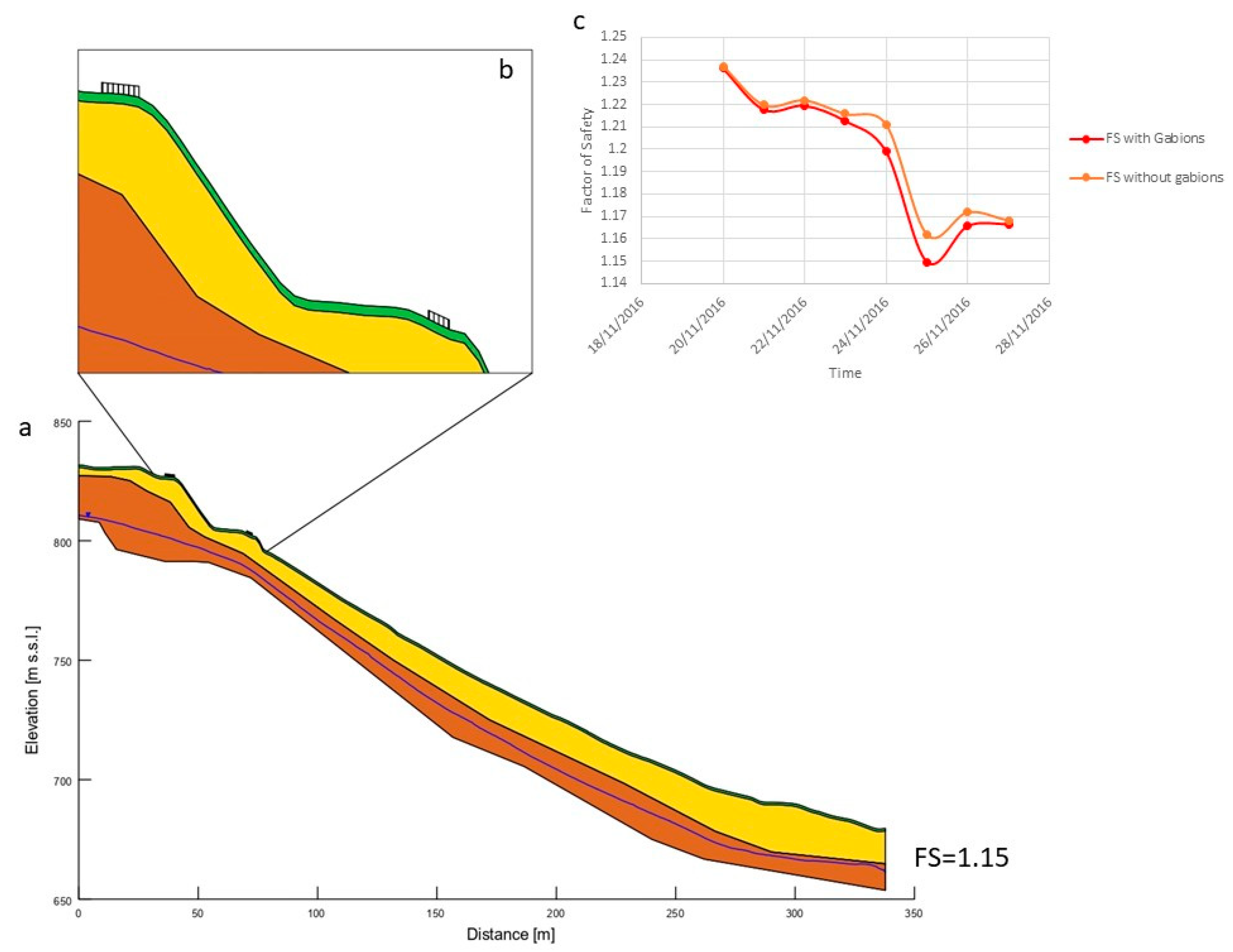
• the slope, due to the steepness of the slope and the nature of the materials, was in limit equilibrium conditions even in dry ground conditions;
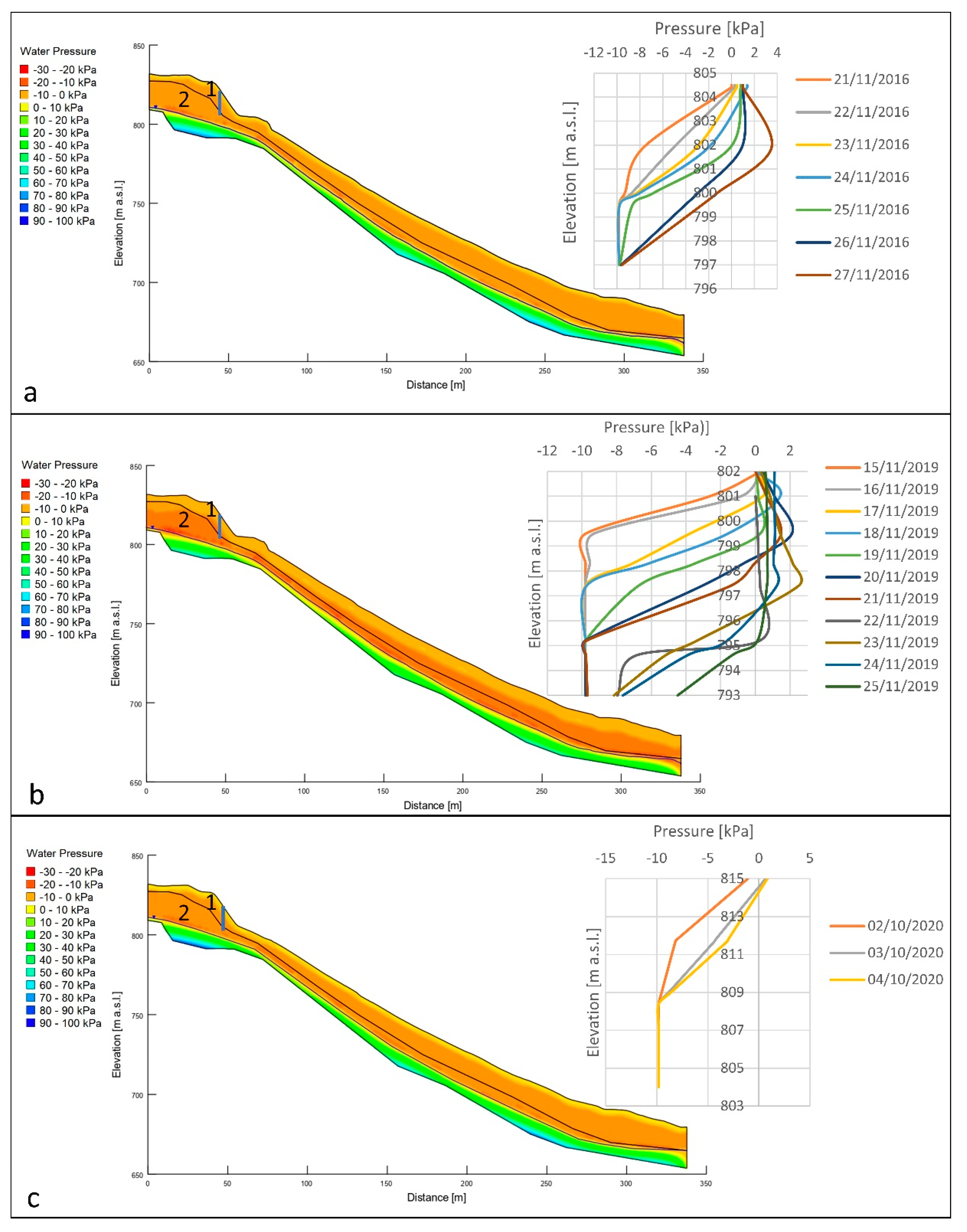
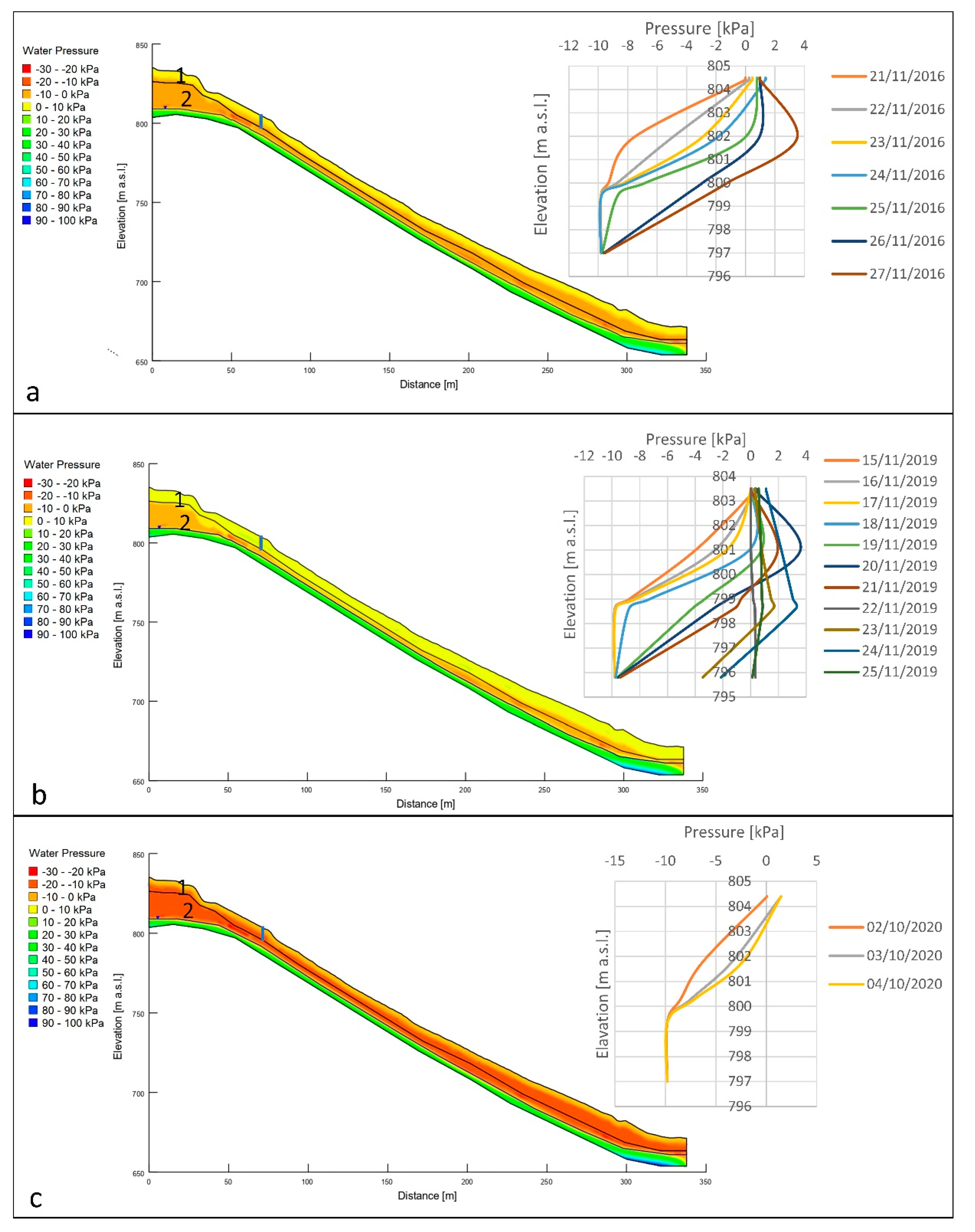
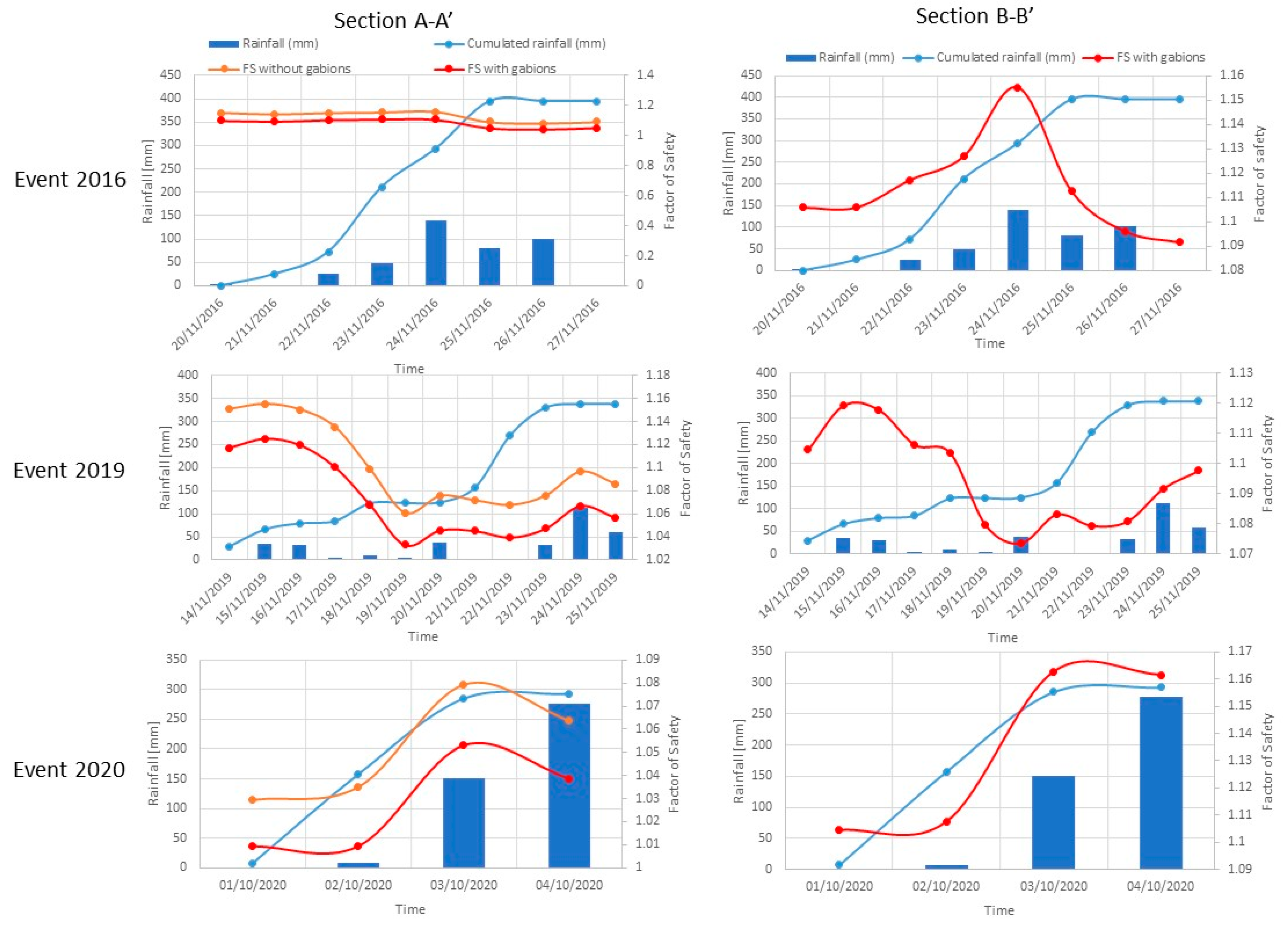
• the filtration analyses conducted for the 2016, 2019 and 2020 events revealed a dynamic of soil saturation from top to bottom, which led to the generation of positive interstitial pressures in the first few metres of soil, and the formation of a saturated front with a maximum thickness of 5 m;
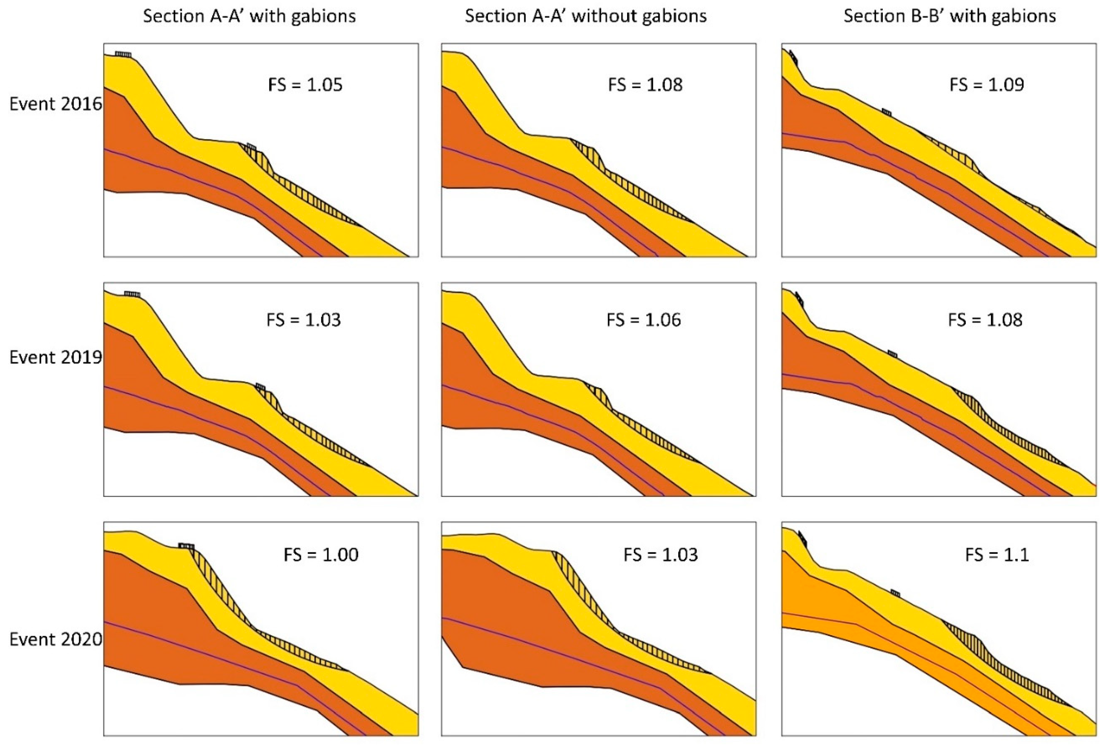
• the stability analyses conducted for the 2016, 2019 and 2020 events showed the development of surface landslides affecting the first few metres of saturated soil;
• the analyses also showed that the presence of the gabion walls played no beneficial role in slope stability, as the FS values in the presence of the works were slightly lower than the values in the absence of the works.

Moreover, the simulation with the presence of bioengineering works showed that a possible grassing of the slope could benefit its stability. This simulation was conducted using the minimum values of root cohesion reported in the literature and without considering the reduction of infiltration due to vegetation, so an intervention in this sense could bring benefits even greater than those estimated.

Finally, the availability of Vs values from geophysical data made it possible to verify the reliability of employing these data in the empirical VS-N-SPT correlations to estimate φ′. This result is important, especially in the first phases of an emergency when civil protection actions must be assessed and a rapid estimation of the further landslide evolution (forward stability analysis) is necessary, but direct N-SPT measures or soil samples are not available.

References

1. Alimohammadlou, Y.; Najafi, A.; Yalcin, A. Landslide Process and Impacts: A Proposed Classification Method. Catena 2013, 104, 219–232. [Google Scholar] [CrossRef]
2. Cepeda, J.; Höeg, K.; Nadim, F. Landslide-Triggering Rainfall Thresholds: A Conceptual Framework. Q. J. Eng. Geol. Hydrogeol. 2010, 43, 69–84. [Google Scholar] [CrossRef]
3. Winter, M.G. Landslide Hazards and Risks to Road Users, Road Infrastructure and Socio-Economic Activity. In Proceedings of the 17th European Conference on Soil Mechanics and Geotechnical Engineering, ECSMGE, Reykjavík, Iceland, 1–6 September 2019; pp. 196–228. [Google Scholar]
4. Milne Cruden, D. Landslide Types and Processes; USGS: Reston, VA, USA, 1996; Volume 247. [Google Scholar]
5. Hungr, O.; Leroueil, S.; Picarelli, L. The Varnes Classification of Landslide Types, an Update. Landslides 2014, 11, 167–194. [Google Scholar] [CrossRef]
6. Chae, B.G.; Park, H.J.; Catani, F.; Simoni, A.; Berti, M. Landslide Prediction, Monitoring and Early Warning: A Concise Review of State-of-the-Art. Geosci. J. 2017, 21, 1033–1070. [Google Scholar] [CrossRef]
7. Gariano, S.L.; Melillo, M.; Peruccacci, S.; Brunetti, M.T. How Much Does the Rainfall Temporal Resolution Affect Rainfall Thresholds for Landslide Triggering? Nat. Hazards 2020, 100, 655–670. [Google Scholar] [CrossRef]
8. Troncone, A.; Pugliese, L.; Conte, E. Rainfall Threshold for Shallow Landslide Triggering Due to Rising Water Table. Water 2022, 14, 2966. [Google Scholar] [CrossRef]
9. Iverson, R.M. Landslide Triggering by Rain Infiltration. Water Resour. Res. 2000, 36, 1897–1910. [Google Scholar] [CrossRef]
10. Yi, X.; Feng, W.; Bai, H.; Shen, H.; Li, H. Catastrophic Landslide Triggered by Persistent Rainfall in Sichuan, China: August 21, 2020, Zhonghaicun Landslide. Landslides 2021, 18, 2907–2921. [Google Scholar] [CrossRef]
11. Duncan, J.M. State of the Art: Limit Equilmrium and Finite-Element Analysis of Slopes 8. J. Geotech. Eng. 1996, 122, 577–596. [Google Scholar] [CrossRef]
12. Memon, Y.A. Comparison Between Limit Equilibrium and Finite Element Methods for Slope Stability Analysis. 2011. Available online: https://www.researchgate.net/publication/329697782_A_Comparison_Between_Limit_Equilibrium_and_Finite_Element_Methods_for_Slope_Stability_Analysis (accessed on 18 March 2022).
13. Innocenti, A.; Pazzi, V.; Borselli, L.; Nocentini, M.; Lombardi, L.; Gigli, G.; Fanti, R. Reconstruction of the Evolution Phases of a Landslide by Using Multi-Layer Back-Analysis Methods. Landslides 2022, 20, 189–207. [Google Scholar] [CrossRef]
14. Mreyen, A.S.; Cauchie, L.; Micu, M.; Onaca, A.; Havenith, H.B. Multiple Geophysical Investigations to Characterize Massive Slope Failure Deposits: Application to the Balta Rockslide, Carpathians. Geophys. J. Int. 2021, 225, 1032–1047. [Google Scholar] [CrossRef]
15. Pazzi, V.; Ciani, L.; Cappuccini, L.; Mattia, C. ERT Investigation of Tumuli: Does the Errors in Locating Electrodes Influence the Resistivity? In Proceedings of the IMEKO TC4 International Conference on Metrology for Archaeology and Cultural Heritage, Florence, Italy, 4–6 December 2019. [Google Scholar]
16. Perrone, A.; Lapenna, V.; Piscitelli, S. Electrical Resistivity Tomography Technique for Landslide Investigation: A Review. Earth Sci. Rev. 2014, 135, 65–82. [Google Scholar] [CrossRef]
17. Pazzi, V.; Morelli, S.; Fanti, R. A Review of the Advantages and Limitations of Geophysical Investigations in Landslide Studies. Int. J. Geophys. 2019, 2019, 2983087. [Google Scholar] [CrossRef]
18. Borecka, A.; Herzig, J.; Durjasz-Rybacka, M. Ground Penetrating Radar Investigations of Landslides: A Case Study in a Landslide in Radziszów. Stud. Geotech. Mech. 2015, 37, 11–18. [Google Scholar] [CrossRef]
19. Hussain, Y.; Schlögel, R.; Innocenti, A.; Hamza, O.; Iannucci, R.; Martino, S.; Havenith, H.B. Review on the Geophysical and UAV-Based Methods Applied to Landslides. Remote Sens. 2022, 14, 4564. [Google Scholar] [CrossRef]
20. Imani, P.; Abd El-Raouf, A.; Tian, G. Landslide Investigation Using Seismic Refraction Tomography Method: A Review. Ann. Geophys. 2021, 64, SE657. [Google Scholar] [CrossRef]
21. Lapenna, V.; Perrone, A. Time-Lapse Electrical Resistivity Tomography (TL-ERT) for Landslide Monitoring: Recent Advances and Future Directions. Appl. Sci. 2022, 12, 1425. [Google Scholar] [CrossRef]
22. Pazzi, V.; Tanteri, L.; Bicocchi, G.; D’Ambrosio, M.; Caselli, A.; Fanti, R. H/V Measurements as an Effective Tool for the Reliable Detection of Landslide Slip Surfaces: Case Studies of Castagnola (La Spezia, Italy) and Roccalbegna (Grosseto, Italy). Phys. Chem. Earth 2017, 98, 136–153. [Google Scholar] [CrossRef]
23. Whiteley, J.S.; Chambers, J.E.; Uhlemann, S.; Boyd, J.; Cimpoiasu, M.O.; Holmes, J.L.; Inauen, C.M.; Watlet, A.; Hawley-Sibbett, L.R.; Sujitapan, C.; et al. Landslide Monitoring Using Seismic Refraction Tomography—The Importance of Incorporating Topographic Variations. Eng. Geol. 2020, 268. [Google Scholar] [CrossRef]
24. Ullah, F.; Su, L.J.; Alam, M.; Cheng, L.; Rehman, M.U.; Asghar, A.; Hussain, G. Landslide Stability Investigation and Subsurface Deformation Mapping by Optimizing Low-Frequency GPR: A Mega Rainfall Susceptible Landslide Case Study (Gilgit Baltistan, Pakistan). Bull. Eng. Geol. Environ. 2022, 81, 373. [Google Scholar] [CrossRef]
25. Rezaei, S.; Shooshpasha, I.; Rezaei, H. Empirical Correlation between Geotechnical and Geophysical Parameters in a Landslide Zone (Case Study: Nargeschal Landslide). Earth Sci. Res. J. 2018, 22, 195–204. [Google Scholar] [CrossRef]
26. Nakamura, Y. A Method for Dynamic Characteristics Od Subsurface Using Microtremor on the Ground Surface; Quaterly Reports; Railway Technical Research Institute: Tokyo, Japan, 1989; Volume 30. [Google Scholar]
27. Fiorucci, M.; Martino, S.; Della Seta, M.; Lenti, L.; Mancini, A. Seismic Response of Landslides to Natural and Man-Induced Ground Vibrations: Evidence from the Petacciato Coastal Slope (Central Italy). Eng. Geol. 2022, 309, 106826. [Google Scholar] [CrossRef]
28. Hussain, Y.; Cardenas-Soto, M.; Uagoda, R.; Martino, S.; Sanchez, N.P.; Moreira, C.A.; Martinez-Carvajal, H. Shear Wave Velocity Estimation by a Joint Inversion of Hvsr and F-k Curves under Diffuse Field Assumption: A Case Study of Sobradinho Landslide. Anu. Inst. Geocienc. 2019, 42, 742–750. [Google Scholar] [CrossRef]
29. Noguchi, T.; Nishimura, I.; Kagawa, T. Estimation of subsurface structure of landslide area based on microtremor observation in the hojoshima, nawashiro and amedaki area, Tottori, Japan. Int. J. GEOMATE 2021, 21, 48–53. [Google Scholar] [CrossRef]
30. Pazzi, V.; Di Filippo, M.; Di Nezza, M.; Carlà, T.; Bardi, F.; Marini, F.; Fontanelli, K.; Intrieri, E.; Fanti, R. Integrated Geophysical Survey in a Sinkhole-Prone Area: Microgravity, Electrical Resistivity Tomographies, and Seismic Noise Measurements to Delimit Its Extension. Eng. Geol. 2018, 243, 282–293. [Google Scholar] [CrossRef]
31. Kannaujiya, S.; Chattoraj, S.L.; Jayalath, D.; Champati ray, P.K.; Bajaj, K.; Podali, S.; Bisht, M.P.S. Integration of Satellite Remote Sensing and Geophysical Techniques (Electrical Resistivity Tomography and Ground Penetrating Radar) for Landslide Characterization at Kunjethi (Kalimath), Garhwal Himalaya, India. Nat. Hazards 2019, 97, 1191–1208. [Google Scholar] [CrossRef]
32. Levashov, S.P.; Bozhezha, D. 21001 Groundwater Flow Studies by EM and GPR Methods for Landslide Zones Prediction. Geoinformatics 2021, 2021, 1–7. [Google Scholar]
33. Stumpf, T.; Bigman, D.P.; Day, D.J. Mapping Complex Land Use Histories and Urban Renewal Using Ground Penetrating Radar: A Case Study from Fort Stanwix. Remote Sens. 2021, 13, 2478. [Google Scholar] [CrossRef]
34. Tandon, R.S.; Gupta, V.; Venkateshwarlu, B.; Joshi, P. An Assessment of Dungale Landslide Using Remotely Piloted Aircraft System (RPAS), Ground Penetration Radar (GPR), and Slide & RS2 Softwares. Nat. Hazards 2022, 113, 1017–1042. [Google Scholar] [CrossRef]
35. Velayudham, J.; Kannaujiya, S.; Sarkar, T.; Champati ray, P.K.; Taloor, A.K.; Singh Bisht, M.P.; Chawla, S.; Pal, S.K. Comprehensive Study on Evaluation of Kaliasaur Landslide Attributes in Garhwal Himalaya by the Execution of Geospatial, Geotechnical and Geophysical Methods. Quat. Sci. Adv. 2021, 3, 100025. [Google Scholar] [CrossRef]
36. Sestras, P.; Bilașco, Ș.; Roșca, S.; Veres, I.; Ilies, N.; Hysa, A.; Spalević, V.; Cîmpeanu, S.M. Multi-Instrumental Approach to Slope Failure Monitoring in a Landslide Susceptible Newly Built-Up Area: Topo-Geodetic Survey, UAV 3D Modelling and Ground-Penetrating Radar. Remote Sens. 2022, 14, 5822. [Google Scholar] [CrossRef]
37. Zhang, D.; Li, J.; Liu, S.; Wang, G. Multi-Frequencies GPR Measurements for Delineating the Shallow Subsurface Features of the Yushu Strike Slip Fault. Acta Geophys. 2019, 67, 501–515. [Google Scholar] [CrossRef]
38. Xie, P.; Wen, H.; Xiao, P.; Zhang, Y. Evaluation of Ground-Penetrating Radar (GPR) and Geology Survey for Slope Stability Study in Mantled Karst Region. Env. Earth Sci. 2018, 77, 122. [Google Scholar] [CrossRef]
39. GeoStudio, 2020. SEEP/W Model and User Manual; Geo-Slope International: Calgary, AB, Canada, 2020. [Google Scholar]
40. GeoStudio, 2020. SLOPE/W Model and User Manual; Geo-Slope International: Calgary, AB, Canada, 2020. [Google Scholar]
41. Morgenstern, N.R.; Price, V.E.; George, G.; London, S. The Analysis of the Stability of General Slip Surfaces the Institution of Civil Engineers the Rights of Publication and of Translation are Reserved. Géotechnique 1965, 15, 79–93. [Google Scholar] [CrossRef]
42. Agostini, A.; Tofani, V.; Nolesini, T.; Gigli, G.; Tanteri, L.; Rosi, A.; Cardellini, S.; Casagli, N. A New Appraisal of the Ancona Landslide Based on Geotechnical Investigations and Stability Modelling. Q. J. Eng. Geol. Hydrogeol. 2014, 47, 29–44. [Google Scholar] [CrossRef]
43. Casagli, N.; Dapporto, S.; Ibsen, M.L.; Tofani, V.; Vannocci, P. Analysis of the Landslide Triggering Mechanism during the Storm of 20th-21st November 2000, in Northern Tuscany. Landslides 2006, 3, 13–21. [Google Scholar] [CrossRef]
44. Nocentini, M.; Tofani, V.; Gigli, G.; Fidolini, F.; Casagli, N. Modeling Debris Flows in Volcanic Terrains for Hazard Mapping: The Case Study of Ischia Island (Italy). Landslides 2015, 12, 831–846. [Google Scholar] [CrossRef]
45. Comune di Fontaneimore. Available online: https://www.comune.fontainemore.ao.it/it-it/home (accessed on 19 January 2023).
46. Segoni, S.; Barbadori, F.; Gatto, A.; Casagli, N. Application of Empirical Approaches for Fast Landslide Hazard Management: The Case Study of Theilly (Italy). Water 2022, 14, 3485. [Google Scholar] [CrossRef]
47. GeoNavigatore SCT. Available online: https://mappe.partout.it/pub/geocartageo/index.html (accessed on 19 January 2023).
48. Okada, H.; Suto, K. The Microtremor Survey Methods; Society of Exploration Geophysicists: Houston, TX, USA, 2003. [Google Scholar]
49. del Gaudio, V.; Muscillo, S.; Wasowski, J. What We Can Learn about Slope Response to Earthquakes from Ambient Noise Analysis: An Overview. Eng. Geol. 2014, 182, 182–200. [Google Scholar] [CrossRef]
50. Molnar, S.; Sirohey, A.; Assaf, J.; Bard, P.Y.; Castellaro, S.; Cornou, C.; Cox, B.; Guillier, B.; Hassani, B.; Kawase, H.; et al. A Review of the Microtremor Horizontal-to-Vertical Spectral Ratio (MHVSR) Method. J. Seism. 2022, 26, 653–685. [Google Scholar] [CrossRef]
51. Castellaro, S.; Mulargia, F. The Effect of Velocity Inversions on H/V. Pure Appl. Geophys. 2009, 166, 567–592. [Google Scholar] [CrossRef]
52. Al-Fares, W.; Bakalowicz, M.; Guérin, R.; Dukhan, M. Analysis of the Karst Aquifer Structure of the Lamalou Area (Hérault, France) with Ground Penetrating Radar. J. Appl. Geophys. 2002, 51, 97–106. [Google Scholar] [CrossRef]
53. Huisman, J.A.; Snepvangers, J.J.J.C.; Bouten, W.; Heuvelink, G.B.M. Mapping Spatial Variation in Surface Soil Water Content: Comparison of Ground-Penetrating Radar and Time Domain Reflectometry. J. Hydrol. 2002, 269, 194–207. [Google Scholar] [CrossRef]
54. Nichol, D.; Lenham, J.W.; Reynolds, J.M. Application of ground-penetrating radar to investigate the effects of badger setts on slope stability at St Asaph Bypass, North Wales. Q. J. Eng. Geol. Hydrogeol. 2003, 36, 143–153. [Google Scholar] [CrossRef]
55. Sass, O.; Bell, R.; Glade, T. Comparison of GPR, 2D-Resistivity and Traditional Techniques for the Subsurface Exploration of the Öschingen Landslide, Swabian Alb (Germany). Geomorphology 2008, 93, 89–103. [Google Scholar] [CrossRef]
56. Zajc, M.; Pogačnik, Ž.; Gosar, A. Ground Penetrating Radar and Structural Geological Mapping Investigation of Karst and Tectonic Features in Flyschoid Rocks as Geological Hazard for Exploitation. Int. J. Rock Mech. Min. Sci. 2014, 67, 78–87. [Google Scholar] [CrossRef]
57. Martínez, J.; Rey, J.; Gutiérrez, L.M.; Novo, A.; Ortiz, A.J.; Alejo, M.; Galdón, J.M. Electrical Resistivity Imaging (ERI) and Ground-Penetrating Radar (GPR) Survey at the Giribaile Site (Upper Guadalquivir Valley; Southern Spain). J. Appl. Geophy. 2015, 123, 218–226. [Google Scholar] [CrossRef]
58. Baryshnikov, V.D.; Khmelin, A.P.; Denisova, E.V. GPR Detection of Inhomogeneities in Concrete Lining of Underground Tunnels. J. Min. Sci. 2014, 50, 25–32. [Google Scholar] [CrossRef]
59. Alsharahi, G.; Faize, A.; Maftei, C.; Driouach, A. GPR Application for Risks Detection in Subsurface Engineering Construction Projects. Ovidius Univ. Ann. Constanta—Ser. Civ. Eng. 2019, 21, 51–58. [Google Scholar] [CrossRef]
60. Grandjean, G.; Gourry, J.C.; Bitri, A. Evaluation of GPR Techniques for Civil-Engineering Applications: Study on a Test Site. J. Appl. Geophys. 2000, 45, 141–156. [Google Scholar] [CrossRef]
61. Daniels, J.J. Fundamentals of Ground Penetrating Radar; Society of Exploration Geophysicists: Denver, CO, USA, 1989; pp. 62–142. [Google Scholar]
62. Neal, A. Ground-Penetrating Radar and Its Use in Sedimentology: Principles, Problems and Progress. Earth Sci. Rev. 2004, 66, 261–330. [Google Scholar] [CrossRef]
63. Rasol, M.; Pérez-Gracia, V.; Fernandes, F.M.; Pais, J.C.; Santos-Assunçao, S.; Roberts, J.S. Ground Penetrating Radar System: Principles. In Handbook of Cultural Heritage Analysis; Springer International Publishing: Cham, Switzerland, 2022; pp. 705–738. [Google Scholar]
64. Schrott, L.; Sass, O. Application of Field Geophysics in Geomorphology: Advances and Limitations Exemplified by Case Studies. Geomorphology 2008, 93, 55–73. [Google Scholar] [CrossRef]
65. Mellett, J.S. I FFLIEI GEI PI 51C5 Ground Penetrating Radar Applications in Engineering, Environmental Management, and Geology; Elsevier: Amsterdam, The Netherlands, 1995; Volume 33. [Google Scholar]
66. Sonkamble, S.; Chandra, S. GPR for Earth and Environmental Applications: Case Studies from India. J. Appl. Geophy. 2021, 193, 104422. [Google Scholar] [CrossRef]
67. Marto, A.; Soon, T.C.; Kasim, F.; Suhatril, M. A correlation of shear wave velocity and standard penetration resistance. Electron. J. Geotech. Eng. 2013, 18, 463–471. [Google Scholar]
68. Brandenberg, S.J.; Bellana, N.; Shantz, T. Shear wave velocity as function of standard penetration test resistance and vertical effective stress at California bridge sites. Soil Dyn. Earthq. Eng. 2010, 30, 1026–1035. [Google Scholar] [CrossRef]
69. Sil, A.; Haloi, J. Empirical correlations with standard penetration test (SPT)-N for estimating shear wave velocity applicable to any region. Int. J. Geosynth. Ground Eng. 2017, 3, 22 . [Google Scholar] [CrossRef]
70. Ohsaki, Y.; Iwasaki, R. On Dynamic Shear Moduli and Poisson’s Ratios of Soil Deposits. Soils Found. 1973, 13, 61–73. [Google Scholar] [CrossRef]
71. Ohta, Y.; Goto, N. Empirical Shear Wave Velocity Equations in Terms of Characteristic Soil Indexes. Earthq. Eng. Struct. Dyn. 1978, 6, 167–187. [Google Scholar] [CrossRef]
72. Imai, T.; Yoshimura, Y. The Relation of Mechanical Properties of Soils to P and S-Wave Velocities for Ground in Japan; Technical Note OYO Corporation: Tokyo, Japan, 1975. [Google Scholar]
73. Lee, S.H.H. Regression Models of Shear Wave Velocities in Taipei Basin. J. Chin. Inst. Eng. 1990, 13, 519–532. [Google Scholar] [CrossRef]
74. Jafari, M.K.; Asghari, A.; Rahmani, I. Empirical Correlation between Shear Wave Velocity (Vs) and SPT-N Value for South of Tehran Soils. In Proceedings of the 4th International Conference on Civil Engineering, Tehran, Iran. 1997. [Google Scholar]
75. Skempton, A.W. Standard Penetration Test Procedures and the Effects in Sands of Overburden Pressure, Relative Density, Particle Size, Ageing and Overconsolidation. Geotechnique 1986, 36, 425–447. [Google Scholar] [CrossRef]
76. Mayne, P.W.; Rix, G.J. Correlations between shear wave velocity and cone tip resistance in natural clays. Soils Found. 1995, 35, 107–110. [Google Scholar] [CrossRef] [PubMed]
77. Anbazhagan, P.; Parihar, A.; Rashmi, H.N. Review of Correlations between SPT N and Shear Modulus: A New Correlation Applicable to Any Region. Soil Dyn. Earthq. Eng. 2012, 36, 52–69. [Google Scholar] [CrossRef]
78. Ataee, O.; Moghaddas, N.H.; Lashkaripour, G.R. Estimating Shear Wave Velocity of Soil Using Standard Penetration Test (SPT) Blow Counts in Mashhad City. J. Earth Syst. Sci. 2019, 128, 66. [Google Scholar] [CrossRef]
79. Esfehanizadeh, M.; Nabizadeh, F.; Yazarloo, R. Correlation between Standard Penetration (N SPT) and Shear Wave Velocity (V S) for Young Coastal Sands of the Caspian Sea. Arab. J. Geosci. 2015, 8, 7333–7341. [Google Scholar] [CrossRef]
80. Madun, A.; Tajuddin, S.A.A.; Abdullah, M.E.; Abidin, M.H.Z.; Sani, S.; Siang, A.J.L.M.; Yusof, M.F. Convertion Shear Wave Velocity to Standard Penetration Resistance. In Proceedings of the IOP Conference Series: Materials Science and Engineering ; Institute of Physics Publishing: Bristol, UK, 2016; Volume 136. [Google Scholar]
81. Maheswari, R.U.; Boominathan, A.; Dodagoudar, G.R. Use of Surface Waves in Statistical Correlations of Shear Wave Velocity and Penetration Resistance of Chennai Soils. Geotech. Geol. Eng. 2010, 28, 119–137. [Google Scholar] [CrossRef]
82. Sun, C.G.; Cho, C.S.; Son, M.; Shin, J.S. Correlations Between Shear Wave Velocity and In-Situ Penetration Test Results for Korean Soil Deposits. Pure Appl. Geophys. 2013, 170, 271–281. [Google Scholar] [CrossRef]
83. Tsiambaos, G.; Sabatakakis, N. Empirical Estimation of Shear Wave Velocity from in Situ Tests on Soil Formations in Greece. Bull. Eng. Geol. Environ. 2011, 70, 291–297. [Google Scholar] [CrossRef]
84. Madiai, C.; Simoni, G. Shear Wave Velocity-Penetration Resistance Correlation for Holocene and Pleistocene Soils of an Area in Central Italy. In Proceedings of the 2nd International Conference on Geotechnical and Geophysical Site Characterization, Porto, Portugal; 2004; pp. 1687–1694. [Google Scholar]
85. Jamiolkowski, M.; Ghionna, V.N.; Lancellotta, R.; Pasqualini, E. New correlations of penetration tests for design practice. In Penetration Testing 1988: Proceedings of the First International Symposium on Penetration Testing 1988, ISOPT-1, Orlando, FL, USA, 20–24 March 1988; De Ruiter, J., Ed.; Brookfield: Rotterdam, The Netherlands; Volume 1, pp. 263–296.
86. Nassaji, F.; Kalantari, B. SPT Capability to Estimate Undrained Shear Strength of Fine-Grained Soils of Tehran, Iran. Electron. J. Geotech. Eng. 2011, 16, 1229–1238. [Google Scholar]
87. Duong, T.H. Effects of Spt Numbers on Liquefaction Potential Assessment of Fine Soil. In Proceedings of the Lecture Notes in Civil Engineering; Springer: Cham, Switzerland, 2020; Volume 80, pp. 691–699. [Google Scholar]
88. ASTM D2217-85; Standard Practice for Wet Preparation of Soil Samples for Particle-Size Analysis and Determination of Soil Constants (Withdrawn 2007). ASTM International: West Conshohocken, PA, USA, 1998.
89. Amoozegar, A. Compact Constant Head Permeameter: A Convenient Device for Measuring Hydraulic Conductivity. In Advances in Measurement of Soil Physical Properties: Bringing Theory into Practice; Wiley: Hoboken, NJ, USA, 2012; pp. 31–42. ISBN 9780891189251. [Google Scholar]
90. Bicocchi, G.; Tofani, V.; D’Ambrosio, M.; Tacconi-Stefanelli, C.; Vannocci, P.; Casagli, N.; Lavorini, G.; Trevisani, M.; Catani, F. Geotechnical and Hydrological Characterization of Hillslope Deposits for Regional Landslide Prediction Modeling. Bull. Eng. Geol. Environ. 2019, 78, 4875–4891. [Google Scholar] [CrossRef]
91. Tofani, V.; Bicocchi, G.; Rossi, G.; Segoni, S.; D’Ambrosio, M.; Casagli, N.; Catani, F. Soil Characterization for Shallow Landslides Modeling: A Case Study in the Northern Apennines (Central Italy). Landslides 2017, 14, 755–770. [Google Scholar] [CrossRef]
92. Philip, J.R. Approximate Analysis of the Borehole Permeameter in Unsaturated Soil. Water Resour. Res. 1985, 21, 1025–1033. [Google Scholar] [CrossRef]
93. ASTM D3080/D3080M; Direct Shear Test of Soils under Consolidated Drained Conditions. ASTM International: West Conshohocken, PA, USA, 2011.
94. Vannocci, P.; Segoni, S.; Masi, E.B.; Cardi, F.; Nocentini, N.; Rosi, A.; Bicocchi, G.; D’Ambrosio, M.; Nocentini, M.; Lombardi, L.; et al. Towards a National-Scale Dataset of Geotechnical and Hydrological Soil Parameters for Shallow Landslide Modeling. Data 2022, 7, 37. [Google Scholar] [CrossRef]
95. ASTM-D1586; Standard Test Method for Standard Penetration Test (SPT) and Split-Barrel Sampling of Soils. ASTM International: West Conshohocken, PA, USA, 2011.
96. Kruse, E.; Eslamian, S.; Ostad-Ali-Askari, K.; Hosseini-Teshnizi, S.Z. Borehole Investigations. Encycl. Earth Sci. Ser. 2018, PartF3. [Google Scholar] [CrossRef]
97. Darcy, H. Les Fontaines Publiques de La Ville de Dijon Exposition et Application; Victor Dalmont.: Paris, France, 1856. [Google Scholar]
98. Childs, E.C.; Collis-George, N. The Permeability of Porous Materiald. Proc. R. Soc. London. Ser. A. Math. Phys. Sci. 1950, 201, 392–405. [Google Scholar]
99. Richards, L.A. Capillary Conduction of Liquids through Porous Mediums. Physics 1931, 1, 318–333. [Google Scholar] [CrossRef]
100. Fredlund, D.G.R.H. Soil Mechanics for Unsaturated Soils; John Wiley & Sons, Inc.: Hoboken, NJ, USA, 1993. [Google Scholar]
101. Vanapalli, S.K.; Fredlund, D.G.; Pufahl, D.E.; Clifton, A.W. Model for the Prediction of Shear Strength with Respect to Soil Suction. Can. Geotech. J. 1996, 33, 379–392. [Google Scholar] [CrossRef]
102. Kanai, K. Improved Empirical Formula for the Characteristics of Strong Earthquake Motions, Proceedings; Japan Earthquake Engineering Symposium: Tokyo, Japan, 1966; pp. 1–4. [Google Scholar]
103. Shibata, T. Analysis of Liquefaction of Saturated Sand during Cyclic Loading. Disaster Prevention Res. Inst. Bull. 1970, 13, 563–570. [Google Scholar]
104. Ohba, S.; Toriumi, I. Dynamic Response Characteristics of Osaka Plain. In Proceedings of the Annual Meeting, A.I.J. (in Japanese), Tokyo, Japan, 5–7 December 1970. [Google Scholar]
105. Ohta, T.; Hara, A.; Niwa, M.; Sakano, T. Elastic Shear Moduli as Estimated from N-Value. In Proceedings of the Proc. 7th Ann. Convention of Japan Society of Soil Mechanics and Foundation Engineering, Tokyo, Japan, July 1972; pp. 265–268. [Google Scholar]
106. Imai, T.; Fumoto, H.; Yokota, K. The Relation of Mechanical Properties of Soils to P-and S-Wave Velocities in Japan. In Proceedings of the Fourth Japanese Earthquake Engineering Symposium, Tokyo, Japan, 19 January 1975; pp. 86–96. [Google Scholar]
107. Imai, T.P.; Wave, S. Velocities of the Ground in Japan. In Proceedings of the International Conference on Soil Mechanics and Foundation Engineering, Tokyo, Japan, 10–15 July 1977; pp. 127–132. [Google Scholar]
108. Japan Road Association. Specification and Interpretation of Bridge Design for Highway; Part V Resilient Des; Japan Road Association: Tokyo, Japan, 1980; p. 14. [Google Scholar]
109. Seed, H.; Idriss, I. Evaluation of Liquefaction Potential of Sand Deposits Based on Observations of Performance in Previous Earthquakes. In Proceedings of the Conference on In Situ Testing to Evaluate Liquefaction Susceptibility; ASCE: St. Louis, MO, USA, 1981. preprint. pp. 81–544. [Google Scholar]
110. Sykora, D.W.; Stokoe, K.H., II. Correlations of In Situ Measurements in Sands of Shear Wave Velocity, Soil Characteristics, and Site Conditions. In Report GR83–3; Civil Engineering Department, University of Texas: Austin, TX, USA, 1983. [Google Scholar]
111. Lin, J.S.; Deng, J.G.; Su, Y.A. Application of Finite Element Method in the Analysis of Deep Excavation. Res. Rep. Taiwan Constr. Technol. Res. 1984. [Google Scholar]
112. Leed, S.H.-H. Analysis of the multicollinearity of regression equations of shear wave velocities. Soils Found. 1992, 32, 205–214. [Google Scholar]
113. Jianguo, C.H. Japan Road Association Correlation Analysis of SPT N Values and Cohesion and Internal Angle of a Clay. Soil Eng. Found. 1990, 26, 91–93. [Google Scholar]
114. de Mello, V.F.B. The Standard Penetration Test State of the Art Review. In Proceedings of the 4th Pan-American Conference SMFE Puerto Rico, San Juan, PR, USA, 1971; Volume 1, pp. 1–86. [Google Scholar]
115. Sowers, G.F. Introductory Soil Mechanics and Foundations, 4th ed.; Macmillan, 621: New York, NY, USA, 1979. [Google Scholar]
116. Peck, R.B.; Hanson, W.E.; Thorburn, T.H. Foundation Engineering, 2nd ed.; John Wiley and Sons: New York, NY, USA, 1974; pp. I 13–I 15. [Google Scholar]
117. Meyerhof, G.G. Penetration Tests and Bearing Capacity of Cohesionless Soils. ASCE J. Geotech. Eng. 1956, 82, 866-1–866-19. [Google Scholar] [CrossRef]
118. Hatanaka, M.; Uchida, A. Empirical Correlation between Penetration Resistance and Internal Friction Angle of Sandy Soils. Soils Found. 1996, 36, 1. [Google Scholar] [CrossRef] [PubMed]
119. Wolff, T.F. Pile Capacity Prediction Using Parameter Functions. Predicted and Observed Axial Behavior of Piles, Results of a Pile Prediction Symposium, sponsored by Geotechnical Engineering Division, ASCE, Evanston, Ill., June 1989. ASCE Geotech. Spec. Publ. 1989, 23, 96–106. [Google Scholar]
120. Schmertmann, J.H. Use the SPT to Measure Dynamic Soil Properties?—Yes, But; ASTM International: West Conshohocken, PA, USA, 1978; pp. 341–355. [Google Scholar]
121. De Baets, S.; Poesen, J.; Reubens, B.; Wemans, K.; De Baerdemaeker, J.; Muys, B. Root Tensile Strength and Root Distribution of Typical Mediterranean Plant Species and Their Contribution to Soil Shear Strength. Plant Soil 2008, 305, 207–226. [Google Scholar] [CrossRef]
122. Masi, E.B.; Segoni, S.; Tofani, V. Root Reinforcement in Slope Stability Models: A Review. Geosciences 2021, 11, 212. [Google Scholar] [CrossRef]
Figure 1. (a) Geological map (retrieved from [47] (accessed on 19 January 2023)) of the Theilly landslide (AO, Italy); (b) 2005–2006 aerial image of Theilly slope; (c) 2012 aerial image of Theilly slope; (d) 2018 aerial image of Theilly slope; (e) 2021 aerial image of Theilly slope. Source of the aerial images: [47].
Remotesensing 15 02159 g001
Figure 2. Flowchart of the phases and data needed to reconstruct the geological–geotechnical model of the slope employed in the stability analysis using the GEOSLPE package.
Remotesensing 15 02159 g002
Figure 3. Location of surveys performed. Red dots are the H/V measurements, blue light dots are the point where the material samples were collected, blue dark dot is the borehole, yellow lines indicate the location of GPR tracks, and black lines are the location of the two sections (A-A’ and B-B’) modelled by filtration–stability analysis.
Remotesensing 15 02159 g003
Figure 4. (a) Location of H/V measurements divided into two groups defined as A and B. (b) H/V curves of group A recorded near the crown. (c) H/V curves of group B recorded on the landslide body.
Remotesensing 15 02159 g004
Figure 5. GPR sections taken at different depths: (a) Z = 1.0 m; (b) Z = 2.0 m; (c) Z = 3.0 m; (d) Z = 4.0 m; (e) Z = 5.0 m; and (f) Z = 6.0 m. The colour scale represents the ability of the medium to absorb/let the pulse pass through it.
Remotesensing 15 02159 g005
Figure 6. Mohr–Coulomb failure envelope for samples T1, T3 and T4.
Remotesensing 15 02159 g006
Figure 7. (a) Geological section along the A-A’ profile; and (b) geological section along the B-B’ profile.
Remotesensing 15 02159 g007
Figure 8. Rainfall path of the (a) November 2016; (b) November 2019; and (c) October 2020 events.
Remotesensing 15 02159 g008
Figure 9. (a) Geotechnical slope model along section A–A’ reconstructed along the line of maximum slope for the last landslide event. 1: Layer 1, sand with gravel; 2: Layer 2, weakly gravelly sand; and 3: Layer 3, bedrock. (b) Zoom of the area with the locations of the gabions. (c) The table shows the geotechnical and hydrological parameters of the two modelled layers.
Remotesensing 15 02159 g009
Figure 10. Distribution of interstitial pressures in the slope (Section A–A’) during selected storm phases: (a) November 2016 event; (b) November 2019 event; and (c) October 2020 event. The blue line in each section represents the vertical transect for which interstitial pressure variations were analysed and graphed. 1 Layer 1; and 2 Layer 2.
Remotesensing 15 02159 g010
Figure 11. Distribution of interstitial pressures in the slope (section B–B’) during selected time steps: (a) November 2016 event; (b) November 2019 event; and (c) October 2020 event. The blue line in the image represents the vertical transect for which the changes in interstitial pressures shown in the graphs were analysed. 1 Layer 1; and 2 Layer 2.
Remotesensing 15 02159 g011
Figure 12. Stability analysis of the 3 events under study. For section A–A’, the analysis was carried out in the presence and absence of structural works, and for section B–B’ only in the presence of retaining works. A zoom of the most critical slip surface identified by the modelling is shown in the figure; for the location of the zoom refer to Figure 9.
Remotesensing 15 02159 g012
Figure 13. Variation of the FS of the most critical slip surface in the presence (red) and absence (orange) of gabion walls in relation to rainfall (dark blue) and cumulated rainfall (light blue).
Remotesensing 15 02159 g013
Figure 14. (a) Slope model for stability analysis simulating the effect of root cohesion. (b) Zoom of the area affected by the critical surface in the presence of gabion walls. (c) Variations of the factor of safety for section A–A’ in the presence of a slope grassing intervention. Red line with the presence of gabion walls; orange line in the absence of gabion walls. 1 Grassing layer; 2 Layer 1; and 3 Layer 2.
Remotesensing 15 02159 g014