Article

Multi-LEO Satellite Stereo Winds

1
Carr Astronautics Corporation, Greenbelt, MD 20770, USA
2
NASA Goddard Space Flight Center, Greenbelt, MD 20771, USA
3
Earth System Science Interdisciplinary Center, University of Maryland, College Park, MD 20740, USA
4
Science Systems and Application Inc., Lanham, MD 20706, USA
*
Author to whom correspondence should be addressed.
Remote Sens. 2023, 15(8), 2154; https://doi.org/10.3390/rs15082154
Submission received: 23 February 2023 / Revised: 15 April 2023 / Accepted: 17 April 2023 / Published: 19 April 2023
(This article belongs to the Special Issue Cloud Remote Sensing: Current Status and Perspective)

Abstract

:
The stereo-winds method follows trackable atmospheric cloud features from multiple viewing perspectives over multiple times, generally involving multiple satellite platforms. Multi-temporal observations provide information about the wind velocity and the observed parallax between viewing perspectives provides information about the height. The stereo-winds method requires no prior assumptions about the thermal profile of the atmosphere to assign a wind height, since the height of the tracked feature is directly determined from the viewing geometry. The method is well developed for pairs of Geostationary (GEO) satellites and a GEO paired with a Low Earth Orbiting (LEO) satellite. However, neither GEO-GEO nor GEO-LEO configurations provide coverage of the poles. In this paper, we develop the stereo-winds method for multi-LEO configurations, to extend coverage from pole to pole. The most promising multi-LEO constellation studied consists of Terra/MODIS and Sentinel-3/SLSTR. Stereo-wind products are validated using clear-sky terrain measurements, spaceborne LiDAR, and reanalysis winds for winter and summer over both poles. Applications of multi-LEO polar stereo winds range from polar atmospheric circulation to nighttime cloud identification. Low cloud detection during polar nighttime is extremely challenging for satellite remote sensing. The stereo-winds method can improve polar cloud observations in otherwise challenging conditions.

Graphical Abstract

1. Introduction

Tracking of cloud features from space to derive Atmospheric Motion Vectors (AMVs), or winds, is a long-established and important measurement technique. Operational meteorological agencies around the globe routinely produce satellite wind products using multi-temporal sequences of imagery from a single Geostationary (GEO) satellite [1,2,3,4] or imagery from multiple passes over the poles by Low-Earth Orbiting (LEO) satellites [5,6]. One of the largest sources of errors in satellite wind measurements is the height assignment for a wind vector [7]. Velden and Bedka [8] estimated that height assignment is the dominant factor in satellite wind uncertainty and contributes up to 70% of the total error. Thus, several studies focused on interpreting satellite AMVs as a layer-average variable [9,10,11].
The height of atmospheric clouds and aerosol features is also a key parameter to understand and characterize their impacts on atmospheric dynamical, chemical, and radiative processes. Accurate cloud top height is critical for determining cloud radiation effects and cloud interactions with precipitation and dynamics [12,13,14]. Aerosol plume heights, such as those from wildfires, dust, and volcano eruptions, play a pivotal role in aerosol transport, air quality prediction, and aviation safety [15,16,17].
Light Detection and Ranging (LiDAR) instruments provide accurate measurements of height, but over a narrow swath, or curtain, without full horizontal sampling of the surrounding thermodynamics and cloud/aerosol processes [18,19]. While such sampling by the Aeolus Doppler-wind LiDAR has been shown to have positive impacts on Numerical Weather Prediction (NWP) [20,21,22], its horizontal coverage and 80 km sampling would be less than ideal for many mesoscale process, Planetary Boundary Layer (PBL), and precipitation studies.
The standard practice of assigning height using Infra-Red (IR) brightness temperature requires prior information or assumptions about the atmospheric thermal structure, which can become problematic in the cases where the atmospheric temperature has a weak or inverted vertical gradient [23,24]. Recent work has focused on improving height assignments using stereo methods, which are not new [25] but are now capable of making accurate height measurements thanks to the improved Image Navigation and Registration (INR) of modern observing systems such as the Geostationary Operational Environmental Satellite R series (GOES-R) Advanced Baseline Imager (ABI) with geo-registration accuracy of a few tenths of a pixel [26,27]. Stereo methods unlock information about the vertical dimension by interpreting apparent shifts in feature locations observed from multiple vantage points as a combination of motion and parallax. Our previous work has developed and validated the stereo method using a pair of Geostationary (GEO) satellites [28,29] or a GEO and a Low-Earth Orbiting (LEO) satellite [30,31]. Using a GEO satellite practically limits the application of stereo methods to ±60° latitude and where there is overlapping coverage. This work seeks to develop the stereo method using multiple LEO satellites to allow for polar coverage.
The Multi-angle Imaging SpectroRadiometer (MISR) is a pathfinder instrument on the NASA Terra satellite that is expressly designed for stereoscopy, including stereo cloud-motion wind applications [32,33]. Although MISR has nine angular looks to determine the cloud height and the cross-track wind component, the along-track winds and height parallaxes are coupled and difficult to separate cleanly [34]. By pairing MISR with GEO imagery, as shown by Carr et al., 2018 [30], a joint LEO-GEO wind retrieval can resolve the along-track wind and height ambiguity, achieving a much better accuracy in both AMV and height. The same could be tried by pairing MISR with imagery from another LEO satellite covering the same area; however, the lack of a thermal IR channel limits the usefulness of MISR for polar observing, although interesting observations of Polar Stratospheric Clouds (PSCs) have been made during polar daylight [35]. In the present work, we consider other sensor combinations for polar stereo-wind observations. An especially promising LEO constellation involves the Moderate Resolution Imaging Spectroradiometer (MODIS) on Terra and the Sea and Land Surface Temperature Radiometer (SLSTR) on the Sentinel-3A and -3B satellites, which offers both down- and aft-looking views of the Earth and thermal IR capability [36]. SLSTR is a successor to the Along Track Scanning Radiometer (ATSR) instrument flown on the European Remote Sensing-1 and -2 (ERS-1 and -2) satellites and the Advanced ATSR (AATSR) flown on the Envisat satellite. An operational multi-LEO SLSTR AMV product is under development at EUMETSAT, but its wind height assignments are based on IR methods rather than stereo [37].
Muller et al. [38,39,40] and other investigators [41,42,43,44,45,46,47] have pioneered the LEO stereo method with ASTR, AASTR, and MISR and have proposed future stereo-observing systems; also studied is the use of cloud shadows in Sentinel-3 imagery to measure cloud heights [48]. The contribution of our work is twofold: (i) fusion of information across LEO platforms (i.e., Terra and Sentinel-3) to cleanly separate the cloud height and the cross-track wind and (ii) compensation of small relative image deregistration errors to further improve stereo-wind retrieval accuracy. Section 2 of this paper introduces the multi-LEO approach to stereo-wind observing and identifies several candidate configurations, including SLSTR-MODIS. The remainder of the paper focuses on the SLSTR-MODIS configuration and the polar regions. Results over both the Arctic and Antarctic are presented in Section 3 and the discussions in Section 4 provide validation and identify applications ranging from cloud analysis to polar circulation.

2. Materials and Methods

Our formulation of the multi-satellite or “stereo” winds method designates a geo-registered scene from one satellite as the reference scene and remaps the scenes from the others into the frame of the reference scene. After remapping, each pixel shares the same apparent geographic coordinates across all scenes. Apparent shifts in the locations of patterns between scenes are known as disparities. These disparities are then interpreted by the retrieval algorithm as a combination of geometric parallax due to feature height and horizontal advection (wind) during the time difference between pixel acquisitions. Disparities relative to the reference scene are measured with subpixel precision by interpolation on a surface of normalized cross correlation used to measure the similarity of a pattern with its translated copy. The best correlations are achieved when time differences are small enough so that cloud patterns retain their shapes (typically under 20 min in the cases presented here) and patterns represent features in a dominant atmospheric layer. Geo-registration accuracy is important for this application, as relative registration errors can map to wind vector and height assignment errors.

2.1. Stereo Wind Retrievals

In the GEO-GEO application, we designate one of a multi-temporal triplet of GEO satellite scenes as the reference and extract all pattern templates from it. The Level-1 products from operational GEO environmental satellites, such as GOES, Himawari, and Meteosat, are geo-registered to a reference ellipsoid (e.g., WGS-84 or GRS-80) so that points on the terrain surface will generally show a disparity with a component that is in proportion to the terrain height above the ellipsoid when feature matching between satellites. In the multi-LEO case, the LEO Level-1 products may not be geo-registered to the ellipsoid but instead registered to the terrain surface.
There are two important differences between this multi-LEO stereo-winds study and our previous work [28,29,30,31]. One is that the multi-LEO wind retrievals derive heights with respect to the terrain surface rather than the ellipsoid. Another difference is the level of overdetermination in the retrieval process associated with the multi-LEO measurements. Overdetermination helps to better constrain the retrieval problem and provide a more robust data quality control. The wind retrieval process is fundamentally a fit to model parameters and each disparity brings two scalar pieces of information. If there are N scenes, including the reference one, there are N − 1 such disparities or 2(N − 1) pieces of information. The GEO-GEO legacy retrieval model solves for five parameters: two horizontal wind vector components and a position adjustment with one vertical and two horizontal components. The vertical position adjustment represents the wind vector height and the horizontal position adjustments absorb the parallax shift of the feature, as seen in the reference scene plus any geo-registration errors. Therefore, the GEO-GEO model must have 2(N − 1) > 5 to be overdetermined. This is easily achieved in a GEO-GEO configuration, with three repetitions of a scene from the reference satellite and two repetitions taken from the other satellite for N = 5. Overdetermination all but assures that the residual disparities after the retrieval at each site are not exactly zero. This enables retrieval quality screening based on the residual statistics. Those retrievals for which the residuals are anomalous with respect to the ensemble statistics can be flagged as suspect as their disparities have not been accurately interpreted by the retrieval model in terms of the model states.
On the other hand, the LEO-GEO case may have less overdetermination. If the LEO sensor is MODIS or VIIRS, then three GEO scenes and one LEO scene count for N = 4. This case is only overdetermined in the five-state model by a single scalar observation and the residuals, which sit in a tangent plane on the ellipsoid, tend to elongate in directions perpendicular to the parallax. Moreover, working with a pair or triplet of LEO sensors such as MODIS or VIIRS (N < 4) clearly provides insufficient information from which to retrieve the five states, while being sufficient for non-stereo winds.
To admit the triple-LEO case, we have reformulated the retrieval problem (Appendix A) to only have three states: two wind velocity vector components and the height. The horizontal position for the wind vector is constrained so that the wind vector 3D-position within the atmosphere must lie on the line-of-site between the reference satellite and the center of the feature template on the terrain surface as indicated in Figure 1. In this formulation, we need 2(N − 1) > 3 to be overdetermined and therefore no fewer than three satellites are required for a stereo retrieval. Such triple-LEO configurations can have the ground tracks of all LEO satellites generally parallel to each other (tandem) or one of the satellite ground tracks crossing the other two. VIIRS on the Suomi National Polar-orbiting Partnership (SNPP) satellite and NOAA-20 (N20) plus MODIS-Aqua is an example of the three-satellite tandem arrangement shown in Figure 2, while any two of these three with MODIS-Terra creates a crossing case, as shown in Figure 3.
The retrieval outputs from fitting the disparities are an estimated state vector with three variables (height and horizontal wind velocity) and a 3 × 3 covariance matrix. The covariance matrix provides an uncertainty for the state vector, based on statistics for the observational uncertainties of the disparities. It is useful to identify places where there is poor stereo acuity because of the geometrical arrangement of the lines-of-sight from the satellites to the feature being tracked. In such cases, the diagonal element (i.e., variance) associated with the height state begins to diverge. Figure 4 shows that this happens in both configurations at high latitudes, which is highly undesirable. The crossing case is relatively better than the tandem one but with less area under triple-overlapping coverage and still a small stereo blind spot.

2.2. Multi-Angle Sensing

Multi-angle observations offer a solution to the stereo blind spot problem just described and makes stereo-wind observing in polar regions interesting from an applications’ perspective. Both MISR (on Terra only) and SLSTR on Sentinel-3A and -3B offer such possibilities; however, we focus on SLSTR in this paper because it has relatively larger swaths and IR capabilities, which MISR lacks. The multi-angle IR capability is important at high latitudes because of reduced solar illumination, particularly in polar winter months. Figure 5 shows the SLSTR coverage concept with (almost) nadir and oblique scans. The SLSTR Level-1 product gives geographic coordinates for each sample for each of nine spectral channels, as summarized in Table 1. Table 1 also shows the alignment between the SLSTR and MODIS channels, mapping each SLSTR channel to the MODIS channel with the nearest central wavelength. Overall channel spectral alignment is quite good, with only S5 and S6 central wavelengths narrowly missing inclusion in a MODIS spectral band.
The ground tracks of the two Sentinel-3 satellites and Terra are close enough to enable full-orbit triple overlaps with MODIS-Terra and the nadir and oblique views of at least one of either Sentinel-3A or -3B SLSTR. SLSTR could also be paired with a VIIRS or MODIS-Aqua to provide polar (but not full-orbit) stereo coverage similar to that shown in Figure 3. The oblique views from both Sentinel-3A and -3B SLSTR also overlap in the polar regions, which allows for quadruple overlap without the benefit of MODIS-Terra. In this paper, we consider mainly the single-Sentinel case. In the dual-Sentinel case, we can have N = 4; in the single-Sentinel case with MODIS-Terra, we have N = 3, as just explained. Either single- or dual-Sentinel configurations allow for overdetermined stereo-wind retrievals with the three-state model without stereo blind spots, as will be demonstrated in our results, but the extent of coverage is greater in the single-Sentinel case. We run full orbits for either Sentinel on a NASA cluster and process retrievals for individual or concatenated consecutive reference satellite granules each time. We use Terra as the reference satellite and take advantage of the high accuracy of MODIS geo-registration to calibrate relative registration errors between each SLSTR view and Terra over clear-sky features, as we explain in Section 4. Other investigators have developed techniques to correct for relative registration between SLSTR spectral channels [52].

3. Results

There are 14 to 15 overpasses of each pole by Terra and both Sentinel-3 satellites each day. High-quality stereo winds have been produced over both poles and the descending (daylight) passage across the midlatitudes and equator. The ascending (nighttime) passage has been found to be problematic, possibly due to larger geo-registration errors because of the lack of reflective channel ground control points during the nighttime ascending segment of the Sentinel-3 orbit; however, the focus of this paper is the polar regions. There have been no problems encountered either during polar summer (day) or polar winter (night) using the LWIR and Mid-Wave IR (MWIR). In the LWIR case, MODIS Band 31 is used with SLSTR Band S8. In the MWIR case, MODIS Band 22 is used with SLSTR S7. Visible (VIS) stereo winds have been successfully performed with MODIS Band 1 and SLSTR S2 during polar summers. In the next section, we discuss validation of the polar stereo-wind retrievals using clear-sky terrain and LiDAR and applications for polar stereo winds.
Figure 6 shows an example of an LWIR case over Antarctica (Appendix B shows a full daily cycle for both poles). The orbital periods for the Sentinel-3 satellites (101 min) differ slightly from that of Terra (99 min), so the phasing of a Sentinel-3 overpass with respect to Terra advances each orbit by about 2 min, while Sentinel-3A and -3B remain phase-locked with respect to each other with Sentinel-3B trailing -3A by 40 min. The time difference between the SLSTR oblique and the nadir views is approximately constant at less than 3 min. In general, when the time between the Sentinel-3 and Terra (Δt) is small, then the patterns being tracked have less time to change shape. The method assumes that the tracked patterns are undergoing pure translation, which is an assumption best satisfied in the limit, as Δt tends to zero; the most high-quality matches (as indicated by the peak normalized cross correlation) are found in this limit. However, the wind retrieval precision must depend inversely on |Δt|, meaning it would be better to have a larger |Δt|. There are two Sentinel-3 satellites from which to choose and, when one is either too far or too close to Terra, the other one can be used instead.
LWIR, MWIR, and VIS cases for polar summer and winter are included in the Supplementary Materials as network Common Data Form (netCDF) files.

4. Discussion

In this section, we validate the retrieved stereo winds over the poles using three methods: ground point retrieval statistics, LiDAR layer–height comparisons, and comparisons with reanalysis winds. Finally, we discuss applications for the polar stereo-wind method.

4.1. Validation

4.1.1. Clear-Sky Terrain Features

Patterns that represent terrain features under clear skies are entirely satisfactory for the application of the stereo method [53]. Their retrieved wind speeds should be zero and their heights above the terrain surface should be zero. Deviations from ideal are indicative of the accuracy of the retrievals. In general, one finds numerous ground points on each polar overpass and both their retrieved heights and speeds can have noticeable biases. Ground-point retrievals are readily identified by K-means clustering in speed–height space as the cluster with the least height–speed combination. We use the time difference between the two satellites as the time scale to convert speed to distance units, before quadratically combining it with the height and sorting the clusters. The clustering population is restricted to heights above ground level less than 2 km and speeds less than 1 m/s.
We can see in Figure 7, where the ground-point retrieval statistics have been plotted for each polar overpass during a one-day period, that there is a noticeable bias in all height retrievals after a first pass of processing. It is interesting to look at the disparities for the ground points, which are plotted in Figure 8. Ideally, these disparities should all cluster at the origin, since all the imagery is registered to the terrain surface; however, Figure 8 shows a clear mean offset between the SLSTR nadir and the oblique scenes and the MODIS reference that is indicative of a deregistration between the SLSTR imagery and MODIS.
Because the retrieval algorithm is very sensitive to small relative registration errors between SLSTR and MODIS, it is useful to conduct a second retrieval pass that reprocesses the disparities after being compensated by the means of the errors observed in the first-pass ground points. This is functionally equivalent to using ground control points from MODIS to reregister the SLSTR nadir and oblique scenes to MODIS. Like GOES-R, the MODIS registration to the terrain surface is very accurate (within 60 m [54]). SLSTR data product quality reports are published for each 27-day orbital cycle [55]. Registration errors are typically larger for the oblique view, as is the case for Figure 8.
Figure 9 shows the ground-point retrieval statistics after the second processing pass. The compensation is carried out independently for each polar overpass whenever there is an adequate population of ground points to be found. Figure 10 shows the compensations for each overpass of a full day (14 orbits). Even if no ground points can be found on a given overpass, it could still be useful to compensate for the registration errors using the compensation from a previous orbit. The overall bias in the retrieved heights seen in Figure 7 has been effectively compensated in Figure 9 after the second processing pass. Similarly, the means for the ground-point velocities are closer to zero. It is also interesting to observe that the standard deviations of the ground-point velocities in Figure 9 are smallest when the absolute values of the SLSTR-MODIS time differences are largest. The time difference for the first overpass is −29 min and increases by about 2 min per overpass until it reaches −1 min for overpass 14. The approach just described shares similarities with Fisher and Muller [56], where the registration between the forward and nadir views of ATSR was modeled from tie-point measurements.

4.1.2. LiDAR Layer Heights

Ground-point standard deviations are typically ~200 m in height and ~0.25 m/s in each velocity component and provide an indication of the retrieval accuracy. However, ground points are not clouds and therefore are not tracking winds. The retrieval errors associated with cloud tracking may be larger [57]. LiDAR provides a second means to validate the height retrievals and has been used by other investigators to assess wind height assignments [58]. The ground track of the Cloud-Aerosol Lidar and Infrared Pathfinder Satellite Observations (CALIPSO) satellite, also in a near-polar orbit, will intersect the swath of SLSTR-MODIS stereo winds on every orbit, with the opportunity to collocate stereo winds and LiDAR measurements from the Cloud-Aerosol Lidar with Orthogonal Polarization (CALIOP) instrument (e.g., Figure 6). Specifically, we use the CALIOP cloud-layer Level-2 product, which reports the top and bottom layer heights for up to 10 layers, and collocate each LiDAR curtain site along the CALIPSO ground track where it intersects the stereo swath, as shown in Figure 11. The collocation algorithm considers all reported layers and all LiDAR footprints within a radius of each stereo-wind site, which allows a tolerance for the horizontal resolution of the stereo retrievals (i.e., template size of 32 km), apparent misregistration of the curtain relative to MODIS (including parallax), and motion of cloud features during the interval between the LiDAR pulses and the MODIS reference imagery. The latter is variable, since CALIPSO and Terra have different orbital periods. The best height match across all layers in the collocation window is used. It is expected that the first LiDAR layer will sometimes be a semitransparent layer above the layer being tracked by the stereo method. Additionally, there is a large effective horizontal spatial resolution mismatch between the stereo method that tracks multi-kilometer scale features and the LiDAR that samples in sub-kilometer laser footprints. This means that LiDAR will sometimes sample holes between broken clouds in the stereo pattern being tracked and, since the LiDAR product has a layer height every 1 km along the ground track, there will typically be many LiDAR samples as CALIPSO traverses the stereo-wind template.
Despite the challenges described above, CALIOP provides a useful tool to assess height-retrieval accuracy along with the measured height of clear-sky ground features relative to the terrain surface. Table 2 reports the height errors determined from the ground points and the difference between retrieved height and CALIOP cloud-top height. For each stereo-wind site, we consider the set of all CALIOP layer tops within 32 km of that site (up to 64 samples) and select the layer nearest the stereo height if more than one LiDAR layer is reported. The Median Absolute Difference (MAD) method provides a robust estimate of the mean and standard deviation of the difference between the LiDAR and stereo heights. In some examples, there is significant variation within the collocated CALIOP heights, indicating a heterogenous layer for which it is hard to interpret the LiDAR heights sampled as being representative of the whole stereo feature template. The last columns of Table 2 report the mean and standard deviation across all sites for a full day of the MAD-estimated mean LiDAR–stereo differences at each site, where the population of sites (N) has been restricted to homogenous layers (MAD-estimated standard deviations in the collocated LiDAR heights < 500 m) and within the same layer (absolute difference between LiDAR and stereo heights < 1 km).
Figure 12 conveys an appreciation of the LiDAR–stereo comparison at a qualitative level. It shows two examples of LiDAR versus stereo height for 21 December 2021: an LWIR case over the Arctic and a visible case over the Antarctic. Both show large populations of differences near zero. The LWIR case has more of a positive bias in the central part of its histogram but both cases show asymmetry to the positive side. This is to be expected, since LiDAR may identify a layer height at an optical depth less than that of the imagery.
While LiDAR provides a precision measurement of a layer height at an optical thickness that may be thinner than that of the imagery, the cloud top is not necessarily the relevant height for the wind assignment. The stereo method uses a pattern that may contain objects with a diverse set of heights and the retrieval is based on how that pattern appears to translate in time and with changing viewing perspectives. The height and wind velocity are therefore effective ones that are characteristic of the pattern. Moreover, in low wind shear conditions within an atmospheric layer, either a height assigned based on cloud tops or a pattern height would apply equally well and a difference between the two is not a wind height assignment error. A similar analysis using the Aeolus Doppler wind LiDAR could also be attempted; however, its requirement to observe the dark side of the terminator will limit the opportunities to collocate with MODIS near the poles. The LiDAR standard deviations in Table 2 are consistently larger than those of the ground points, but this may overestimate the stereo-wind errors.

4.1.3. Reanalysis Winds

To validate the retrieved stereo-wind vectors, we use European Center for Medium Range Weather Forecasting (ECMWF) fifth-generation Reanalysis (ERA5) [59] wind profiles for the dates in question, collocated in space and time with the stereo-retrieval sites using a nearest neighbor assignment. The ERA5 model updates hourly and has a grid spacing of 0.25°, which allows for collocation to better ±15 km, so each stereo-wind template will contain a grid point simultaneous to within ±30 min. ERA5 profiles are recorded at 37 distinct pressure levels. The geopotential is provided at each pressure level, from which we calculate the geopotential height. We interpolate a reanalysis wind to compare with each stereo wind at the stereo height using the wind versus the geopotential height at the 37 model levels. Figure 13 provides an example of one comparison and Table 3 provides aggregated statistics across all overpasses of the pole for each case in comparison with ground-point error statistics. The best results correspond to cases where the ERA5 data are most simultaneous with the stereo winds (e.g., Figure 13). The statistics exclude a small outlier population (absolute difference > 15 m/s). The outlier population size depends on the time difference between the stereo and reanalysis winds. In Figure 13, the reanalysis and observed winds are essentially simultaneous and the excluded outlier population is <1%, but, when the difference exceeds 20 min, it can be >3%. The low bias and ~2.5 m/s standard deviation are similar to results found in a study comparing ERA5 with radiosonde winds collected in a field campaign at high latitudes [60]. Another study [34], comparing MISR stereo winds to GOES and MODIS winds, shows similar differences (2–4 m/s) between datasets. The ERA5 comparisons in Table 3 show larger errors than the ground points and are also likely to overestimate the stereo-wind errors.

4.2. Applications

The multi-LEO method developed here improves upon existing operational methods in the polar regions and has important applications to strengthen our understanding of polar weather and climate.

4.2.1. Consistency in Polar Day–Night Cloudiness

The Arctic climate is warming at an alarming rate, nearly four times faster than the rest of the world since 1979 [61]. Polar clouds play a crucial role in the Earth’s climate system, including the Arctic, because of their major influence on surface radiation and subsequent cryospheric/atmospheric thermodynamics. During the summer months, bright white clouds can reflect a large amount of solar radiation back into space and reduce direct solar heating of the polar surfaces. In the winter, polar nighttime clouds can trap heat near the surface and keep the polar region warmer than without them.
In a comparative study of MODIS and CALIOP cloud-mask products, Liu et al., 2010 [62], found that the Arctic cloud cover from the passive IR radiometric method tends to bias low in the presence of Sea Ice Concentration (SIC). Both data sets show that the cloudiness tends to decrease with increased SIC, but MODIS cloudiness decreases at a larger rate due to the systematic low bias. The MODIS cloudiness bias is more pronounced in the nighttime than the daytime measurements, likely because of lacking the visible band in the cloud detection.
Climate models struggle to reproduce the observed Arctic cloud amount and differ significantly between each other, showing larger differences in wintertime than summertime cloudiness [63]. On the other hand, differences also exist between cloud amount from satellite observations and reanalysis data [64]. Thus, reducing uncertainties of the satellite observations in the polar region is critically needed, as a cloud mask is fundamental to retrieving other cloud properties in subsequent data processing. The multi-LEO stereo cloud mask developed in this study from the IR band, which classifies clouds as a feature above the terrain height from the stereo technique, can be used as a new independent data set for polar cloud detection. In addition to its swath coverage, the independence of visible channels and radiometric calibration allows the multi-LEO stereo data to produce consistent cloud observations between day and night for studying diurnal and annual variations.
Stereo methods have been successfully used to discriminate clouds from polar surface backgrounds using ATSR-2 [65]. Here, we exploit the MODIS-SLSTR stereo-wind product to derive a probabilistic cloud mask that classifies whether a tracking template has clouds or is almost all clear using the likelihood ratio between the alternative hypotheses: the template is cloudy or the template is clear. The ground-point clustering algorithm introduced in Section 4.1.1 provides an identification of retrievals over clear-sky terrain. We use these retrievals to establish a Gaussian model for the tri-variate distribution of height and horizontal velocity to compare with a presumed uniform distribution for clouds (a height up to 16 km and speed up to 60 m/s captures almost all retrievals). The likelihood ratio between the Gaussian model and uniform distributions provides the discrimination between clear and cloudy. In the following, we compare stereo-wind classifications to the MODIS Level-2 cloud mask at 2 km resolution [66,67,68] using a known challenging case, polar winter [69,70], as an example. The MODIS cloud mask provides per pixel classifications with the labels: “unknown”, “cloudy”, “uncertain clear”, “probably clear”, and “clear”. In this analysis, we count the number of each for all retrieval templates. There are no instances of the “unknown” label observed, but between ~5% and ~25% for the “uncertain clear” and “probable clear” labels was seen in the polar overpasses. Figure 14 is a density plot of stereo-cloudy/clear likelihood ratio versus the MODIS cloud fraction for each template, considering only templates without “uncertain clear” pixels. The “probably clear” pixels are counted as not cloudy. We can see that most of the population fits in the four corners of the plot. In most cases, the stereo classifier makes a clear choice because there is a rather clear separation between the clear-sky ground cluster and other clusters associated with cloud layers. The corners on the upper right and bottom left are occurrences where MODIS and the stereo method agree. The other corners are where they disagree. Note that the stereo method provides a cloudiness assessment for a template rather than a pixel. It categorizes templates as cloudy, based on trackable cloud features that potentially cover only ~10% of the template.
This example shows how the stereo method can potentially improve or validate cloud-masking datasets from other sensors. Figure 14 omitted templates for which MODIS cloud mask pixels could not be confidently resolved as clear or cloudy (“uncertain clear”). Stereo methods may be useful in their resolution.

4.2.2. Polar Meridional Transport Processes

The multi-LEO stereo cloud winds provide tracking of cloud development and life cycle in the polar region. Atmospheric Rossby waves produce periodical poleward meridional transport, or Warm Air Intrusions (WAIs), as well as equatorward transport, or Cold Air Outbreaks (CAOs), which often lead to different cloud formation and atmospheric responses. During the WAI events in the northern hemisphere, the poleward transport of warm humid air into the Arctic can enhance or prolong sea-ice melt. On the other hand, large-scale CAO events export cold dry air from the Arctic to the midlatitudes, which can cause severe weather in the winter [71].

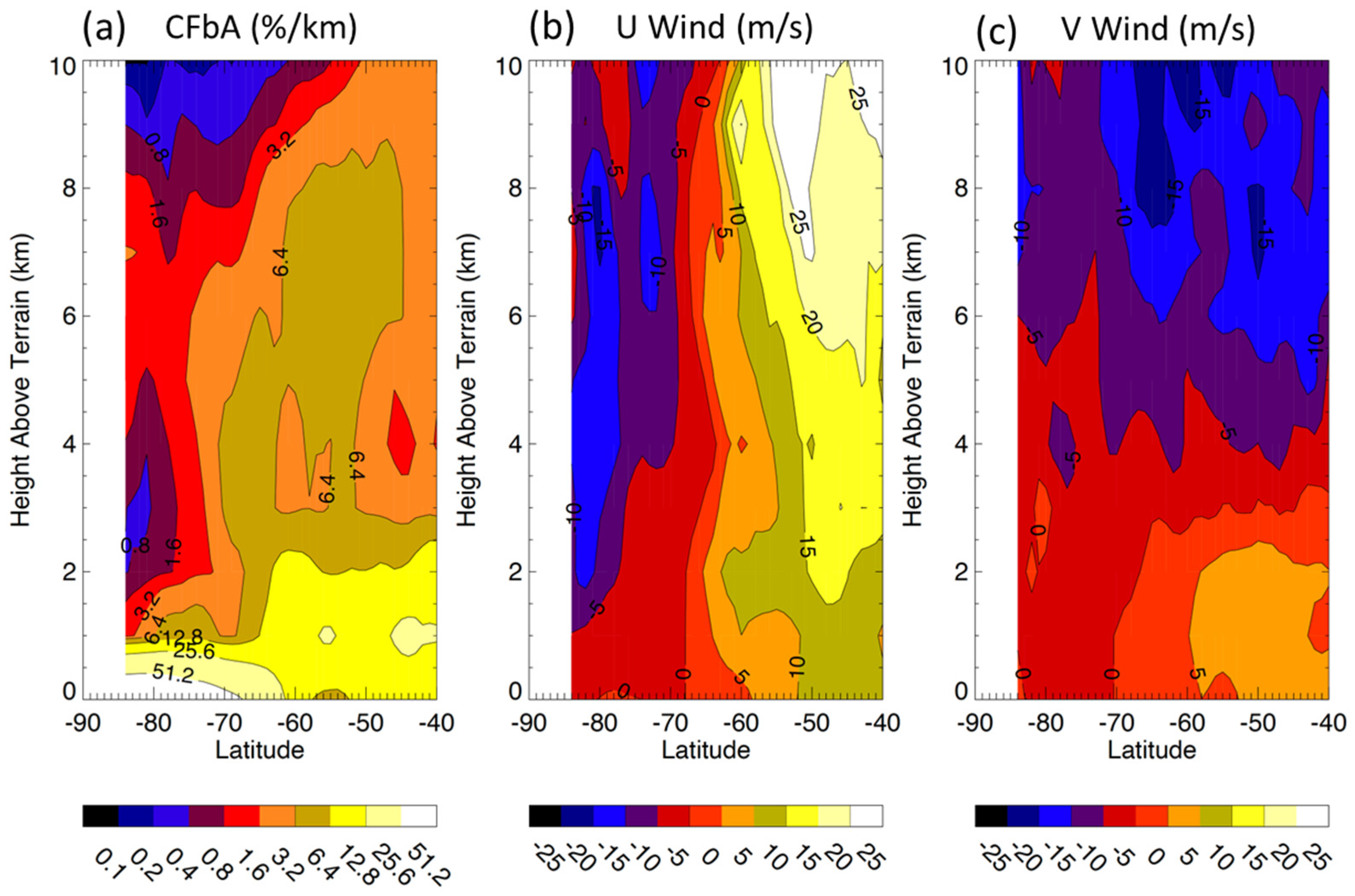
4.2.3. Antarctic Tropospheric Circulation

Antarctica is one of most windy regions in the world and yet the observations there are relatively sparse. To illustrate the mean atmospheric circulation over the Antarctic, we processed 5 days of the LEO-LEO stereo winds from 7 to 11 July 2021. The zonal mean distributions of the 5 day zonal (U) and meridional (V) winds as well as Cloud occurrence Frequency by Altitude (CFbA) are shown in Figure 15. The general circulation in the southern hemisphere polar region is evident in the zonal mean V wind and CFbA. The equatorward and poleward flows are seen in the lower (<3 km) and upper (>5 km) troposphere at latitudes between 40°S and 70°S. This mean meridional circulation results in a descending flow in the Antarctic interior due to mass conservation, which manifests itself as the low CFbA seen in the LEO-LEO stereo observations at latitudes of 75°S poleward. This circulation is also called a polar cell. In addition, CFbA shows more frequent occurrences in the PBL that often tops at ~2 km above the surface at oceanic latitudes between 40°S and 65°S. The cloud-defined PBL top appears to drop sharply at latitudes 65°S–85°S over the Antarctic, where the cold surface and the air descent keep cloud layers low.
The polar descending air is the fundamental driving force of downslope katabatic winds near the surface in the Antarctic. Around the coastal regions, the Antarctic winds are subject to large variations influenced by the katabatic flow and by synoptic perturbations such as cyclones in the Southern Ocean. Figure 16 shows maps of low-level (500–2000 m) winds and their variability from the five days when a cyclone swept through the Southern Ocean. Effects of the cyclone are clearly seen in the wind-speed map that has a low speed near the cyclone center and high values surrounding it. The cyclone generated an average poleward flow near the Peninsula and an equatorward flow near the Ross Sea. The cyclone created strong wind disturbances over Antarctica, as indicated by the enhanced standard deviations in wind speed.

5. Conclusions

The stereo method retrieves both wind velocity and height directly using only geometric information. It is a direct determination of height without any prior assumptions about atmospheric temperature profiles. No synchronization of observations between satellites is required, but pixel times must either be known or accurately modeled. We have developed the stereo-winds method for multi-LEO configurations, permitting stereo-winds coverage of the polar regions. It has been applied to several cases, including three-satellite combinations in tandem and crossing formations. Three satellites orbiting in tandem (e.g., Aqua, NOAA-20, and SNPP; or NOAA-20, -21, and SNPP) can provide full-orbit coverage of the Earth, but there are stereo blind spots where the acuity of the stereo retrieval of height is poor due to the lines-of-sight from each satellite to a common point on the Earth becoming nearly parallel. The acuity is improved when one of the three satellites crosses the path of the other two (e.g., Terra, Aqua, and NOAA-20).
Better quality stereo winds can be produced by pairing a multi-angle sensor (e.g., MISR or SLSTR) with another LEO, because a second satellite is needed to cleanly separate the in-track wind component from the height, even in the case of MISR, which has nine cameras. MISR has visible and near-IR bands only, so it is not well-suited to remote sensing in the polar regions, except during polar summers. SLSTR has only two looks (aft and nadir) but possesses thermal IR bands. We mostly explored the pairing of SLSTR with MODIS for these reasons. MODIS on Terra flies in a train configuration with SLSTR on the Sentinel-3A and -3B satellites. This enables full-orbit coverage with Terra paired with either of the Sentinel-3 satellites. The multi-angle capability of SLSTR assures the lack of stereo blind spots, which is a clear demonstration of the benefit of multi-angle imaging used in tandem with another platform.
The applications in this paper focus on the polar regions and include polar circulation and cloud masking. The zonal and meridional winds over the Antarctic from 5 day stereo-wind retrievals reveal a reasonable general polar-cell circulation pattern in the troposphere and frequent occurrence of PBL clouds at oceanic latitudes between 40°S and 65°S. Polar cloud detection is critical in climate research in other remote sensing applications. This study demonstrates that multi-LEO stereo cloud masks from the IR band can serve as an independent data set for these applications with consistent cloud detection between day and night.
The MODIS-SLSTR combination is limited by the lifetime of Terra; however, MODIS-SLSTR will remain useful for retrospective studies, starting from the Sentinel-3A launch in early 2016 and configurations where the ground track of a Sentinel-3 satellite crosses a JPSS or an SNPP satellite carrying VIIRS will remain viable. Sentinel-3A and -3B paired together can also be used for stereo winds, albeit with less coverage area over the poles; two additional Sentinel-3 satellites are planned to continue the Sentinel-3 mission. Other observing systems are planned that could benefit from the methods described in this paper. Notably, ESA has recently selected Harmony as an Earth Explorer mission. Harmony will consist of a tandem pair of satellites flying in coordination with Sentinel-1. In addition to a bistatic receive-only Synthetic Aperture Radar (SAR) using illumination from Sentinel-1, each satellite will carry a thermal IR multi-angle imager with 300 m resolution [72,73]. The Compact Midwave Imaging System (CMIS) [74] is another sensor with multi-angle IR capability with potential future flight opportunities, flying in tandem pairs or in a train with another series of satellites (e.g., JPSS or MetOp-Second Generation). In most of the work presented here, stereo coverage is limited by the narrow swath of the SLSTR oblique view, which is still larger than that of MISR (740 km versus 380 km). A two-satellite constellation will only cover a small portion of each pole in each orbit (e.g., Figure A1, Figure A2, Figure A3 and Figure A4). This could be sufficient for research purposes, but a larger constellation of low-cost imagers could serve as a cost-effective solution for operational wind products serving NWP objectives. Such constellation concepts are under formulation to meet future weather sensing needs (e.g., as a follow-on to JPSS [75]).
We have validated our stereo-wind retrievals using fixed clear-sky ground points, collocated CALIOP cloud-top heights, and ERA5 reanalysis winds. All validation methods have some nuance to their interpretations. The ground points show the smallest retrieval errors, ~200 m and ~0.25 m/s, but ground points are not clouds borne in the wind and are expected to underestimate wind retrieval errors. Moreover, we use the ground- point disparities to remove biases in the retrievals (~400 m and ~0.25 m/s) that are due to small relative geo-registration errors between MODIS and SLSTR with a second retrieval processing pass; therefore, ground points are not entirely independent measurements of retrieval accuracy. The ground-point disparities are modeled as constant for each polar overpass but may have a more complicated temporal structural to be modeled to improve upon the compensation. More work is needed to fully understand these errors, which can be related directly to height and velocity retrieval errors. Cloud optical depth and inhomogeneity can play a significant role in the cloud-top heights observed by LiDAR and IR sensors [58]. The LiDAR measurements only exist along a narrow path cutting through the retrieval swath that may not representatively sample the cloud tops of a tracking template. Moreover, the LiDAR signal return may be from an optical depth above the effective height of clouds in passive imagery or even from a different layer. It is therefore not surprising to see generally positive biases of several hundred meters between CALIOP layer heights and the stereo retrievals, with ~500 m standard errors. The reanalysis winds are expected to show some differences with observational wind fields, since they are modeled winds on discrete layers and not always simultaneous with the observational winds. Our comparisons with ERA5 are generally unbiased, with ~3 m/s standard errors, which are similar to other comparisons between reanalysis and observational winds [60].
Stereo-wind observations in the polar regions not only facilitate the study of polar atmospheric dynamics but also provide a reliable technique for mapping polar clouds in darkness or when cloud layers are close to the ground. Large uncertainty about cloud cover is a challenging problem in polar regions, with a direct bearing on climate. Consistent polar cloud detection from stereo-wind methods during daytime and nighttime is critical for model evaluation and understanding of the underlying dynamical and radiative processes. We show, as has also been demonstrated with ATSR-2 [65], that stereo methods have potential to contribute to consistent polar day–night cloud detection.

Supplementary Materials

Data supplement is available for download as Carr, James; Wu, Dong; Friberg, Mariel; Summers, Tyler (2023), Polar Stereo Winds, Dryad, Dataset, https://doi.org/10.5061/dryad.rfj6q57g5 (accessed on 19 February 2023).

Author Contributions

Conceptualization, J.L.C. and D.L.W.; methodology, J.L.C. and D.L.W.; software, J.L.C., M.D.F., and T.C.S.; validation, J.L.C.; formal analysis, J.L.C. and D.L.W.; investigation, J.L.C. and D.L.W.; resources, D.L.W.; data curation, T.C.S.; writing—original draft preparation, J.L.C. and D.L.W.; writing—review and editing, J.L.C. and D.L.W.; visualization, J.L.C.; supervision, J.L.C. and D.L.W.; project administration, D.L.W.; funding acquisition, D.L.W. All authors have read and agreed to the published version of the manuscript.

Funding

J.L.C. and T.C.S. received support from NASA Goddard Space Flight Center under the NNG17HP01C contract through Support for Atmospheres, Modeling, and Data Assimilation (SAMDA). Resources supporting this work were provided by the NASA High-End Computing (HEC) Program (NASA program manager: Tsengdar Lee) through the NASA Center for Climate Simulation (NCCS) at Goddard Space Flight Center. D.L.W. received support from NASA’s Terra Project.

Data Availability Statement

Stereo-winds datasets are available in the Supplementary Materials. MODIS and SLSTR Level-1 datasets used for this study are available through the NASA Level-1 and Atmosphere Archive & Distribution System Distributed Active Archive Center (LAADS DAAC) https://ladsweb.modaps.eosdis.nasa.gov/ (accessed on 19 February 2023).

Acknowledgments

Special thanks to Jan-Peter Muller, University College London, for guiding us towards an understanding of the Sentinel-3 Sea and Land Surface Temperature Radiometer (SLSTR) and its data products.

Conflicts of Interest

The authors declare no conflict of interest.

Appendix A

The math model of the retrieval algorithm for the multi-LEO case is adapted from the MISR-GEO [30] and MODIS-GEO [31] models. Each satellite image is assumed to have been remapped into common coordinates (e.g., a polar stereographic projection) so that disparities can be easily found by pattern matching. It is applicable to any constellation of satellites (including only GEO satellites) and sensors with and without multi-angle capabilities. The reduced solution order (three versus the five variables of our other models [28,29,30,31]) allows a solution to be found with fewer observations.
Consider a moving object O (e.g., the cloud shown in Figure 1) and let r n ( O ) be where it appears to rest on the surface (or ellipsoid if imagery is registered to the ellipsoid rather than the terrain surface) as viewed from satellite/look n at the respective observation times t n . Reserve n = 0 to designate the reference scene from which we draw the template. The true position vector for the object O would be r ( O ) = r 0 ( O ) + δ ( t ) , where δ ( t ) is the adjustment needed to position O in 3D space off the surface (or ellipsoid) at time t . We seek to discover δ , for which the component in the direction of the local vertical would be the height assignment and the trajectory of δ that is parallel to the surface of the ellipsoid would represent the wind.
Consider a single disparity pairing for which the matching algorithm has found the coordinates for O as it would appear from satellite/look n were it to sit on the surface (or ellipsoid). The line-of-sight to O for satellite/look n starts at the position vector for the satellite ( R n ) and runs parallel to the vector touching the apparent location of O on the surface (or ellipsoid) r n ( O ) and must run through the 3D location of the object r ( O ) = r 0 ( O ) + δ . Expressed mathematically, there must be some multiplier λ 1 that makes this equation hold:
r 0 ( O ) + δ = λ 1 ( r n ( O ) R n + ϵ n ) + R n .
The apparent position of O on the surface (or ellipsoid) r n ( O ) could not have been determined perfectly, so we have introduced a vector ϵ n in Equation (A1) to make equality hold that we can interpret as deriving from an error or uncertainty in the disparity measurement. Normally, ϵ n should be small. All imagery has been mapped into common coordinates, the point of correspondence is found where the template best matches, the coordinates of the match inverted to determine the latitude and longitude, and finally the apparent position vector ( r n ( O ) ) is calculated. In doing so, r n ( O ) can only rest on the surface (or ellipsoid), so we can consider small deviations in the calculations represented by ϵ n as sitting in the tangent plane at r n ( O ) ; i.e., z ^ n · ϵ n = 0 , where z ^ n is taken to be the local vertical at r n ( O ) . We rearrange Equation (A1) to isolate ϵ n on the left-hand side:
ϵ n = λ   ( r 0 ( O ) R n + δ ) ( r n ( O ) R n ) .
Equation (A2) is used to derive an equation for λ from the constraint z ^ n · ϵ n = 0 ,
λ = z ^ n · ( r n ( O ) R n ) z ^ n · ( r 0 ( O ) R n + δ ) .
Equation (A3) is nonlinear in δ , but given a guess δ 0 for the value of δ , we can linearize it in a Taylor series:
λ   z ^ n · ( r n ( O ) R n ) z ^ n · ( r 0 ( O ) R n + δ 0 ) z ^ n · ( r n ( O ) R n ) ( z ^ n · ( r 0 ( O ) R n + δ 0 ) ) 2 z ^ n · ( δ δ 0 ) .
Substituting λ from Equation (A4) into (A2) and discarding terms higher than linear in δ δ 0 gives an approximate linear measurement model:
ϵ n = A n ( δ 0 ) · ( δ δ 0 ) b n ( δ 0 ) .
The matrix A n ( δ 0 ) and vector b n ( δ 0 ) are defined accordingly (with I as the identity matrix):
A n ( δ 0 ) = λ 0 [ I ( r 0 ( O ) R n + δ 0 ) z ^ n T z ^ n · ( r 0 ( O ) R n + δ 0 ) ] ,  
b n ( δ 0 ) = ( r n ( O ) R n ) λ 0 ( r 0 ( O ) R n + δ 0 ) .
λ 0 = z ^ n · ( r n ( O ) R n ) z ^ n · ( r 0 ( O ) R n + δ 0 ) .  
We next parameterize δ ( t ) = h r 0 ( O ) R 0 ( r 0 ( O ) R 0 ) · z ^ 0 + V · ( t t 0 ) so that at t = t 0 , δ ( t 0 ) is parallel to the line-of-sight from the apparent location in the reference scene to the reference satellite with the height being the projection onto the local vertical z ^ 0 and further require that the wind velocity V is perpendicular to z ^ 0 (i.e., V = V u u ^ 0 + V v v ^ 0 for vectors in the local tangent plane u ^ 0 and v ^ 0 directed towards the east and north, respectively). Substituting for δ into Equation (A5) gives an equation in terms of the three variables or “states” X = [ h   V u   V v ] T :
ϵ n = B n ( δ 0 ) · ( X X 0 ) b n ( X 0 ) ,
with
B n = [ A n r 0 ( O ) R 0 ( r 0 ( O ) R 0 ) · z ^ 0 ,   ( t n t 0 ) A n u ^ 0 ,   ( t n t 0 ) A n v ^ 0 ]

Appendix A.1. Solution by Simple Least Squares

We can solve for X in a least squares sense by minimizing
χ 2 = n = 1 N ϵ n T W n ϵ n .  
A weighting matrix W n has been introduced. It can be the identity matrix for an unweighted solution. This solution to this least-squares problem is the solution to the linear system:
( n = 1 N B n ( X 0 ) T W n B n ( X 0 ) ) ( X X 0 ) = n = 1 N B n ( X 0 ) T W n b n ( X 0 ) .  
To solve for X as a nonlinear problem, we start with a guess X 0 , solve for Δ X = X X 0 , update the guess, and iterate. The solution is considered to have converged once | Δ X | is less than a tolerance. If the measurement errors for the disparities are random and uncorrelated and each is weighted by a W n that is the inverse of the covariance matrix of the measurement uncertainty, then the uncertainty of the estimate for X is described by a covariance matrix P , which is given by the coefficient matrix in Equation (A10):
P = ( n = 1 N B n ( X 0 ) T W n B n ( X 0 ) ) 1 .  
The square roots of the diagonal elements of P can be interpreted as error bars for each of the solved parameters in accordance with the statistical description of the disparity measurement errors.

Appendix A.2. Solution with Priors

The three-state problem can be singular or nearly singular in certain geometrical configurations. An effective means of coping with this problem and retaining the benefit of retrieving some information is to introduce a prior X ˜ for the state vector and a symmetric matrix M that quantifies our uncertainty in the prior information. We introduce the diagonal matrix M 1 and allow (slightly abusively) for it to have zero diagonal values so that we can loosely constrain only the height (make velocity diagonals zero) or velocity (make height diagonal zero). Setting M 1 = 0 will revert to the unconstrained problem. Thus, we modify Equation (A9) and initialize the solution search with X 0 = X ˜ :
χ 2 = n = 1 N ϵ n T W n ϵ n + ( X X ˜ ) T M 1 ( X X ˜ ) .  
The more general form of the solution of an iteration is now
( P 1 + M 1 ) ( X X 0 ) = M 1 ( X ˜ X 0 ) + n = 1 N B n ( X 0 ) T W n b n ( X 0 ) .

Appendix A.3. Solution by Constrained Optimization

Another approach to achieve the same purpose is through constrained optimization with a Lagrange multiplier ( Λ ) in either of two formulations:
χ 2 = n = 1 N ϵ n T W n ϵ n + Λ ( X T g X v c 2 ) ,   or  
χ 2 = n = 1 N ϵ n T W n ϵ n + Λ ( X T k h c ) .  
In the first, the constraint is X T g X = v c 2 , with a “metric” matrix g that can project out the velocity part of the state vector such that the solved-for speed is v c . The idea of constraining the wind is similar to the MINX approach to MISR retrievals [76]. In the second, the constraint is X T k = h c , with a vector k that selects the height part of the state vector such that the solved-for height is h c . Following the usual procedure, Equation (A14a) or (A14b) is solved and the solution is a function of Λ that is in turn determined by solving the constraint. In the respective cases, the equivalents of Equation (A10) are
( P 1 + Λ g ) ( X X 0 ) = n = 1 N B n ( X 0 ) T W n b n ( X 0 ) Λ g X 0 ,   or  
P 1 ( X X 0 ) = n = 1 N B n ( X 0 ) T W n b n ( X 0 ) 1 2 Λ k .  
In the first case, the solution is nonlinear in the Lagrange multiplier and will require a numerical solution. In the second case, the solution is linear in the Lagrange multiplier and the Lagrange multiplier is easily solved from the constraint equation:
Λ = 2 k T P k ( X T k + ( n = 1 N B n ( X 0 ) T W n b n ( X 0 ) ) T P k h c ) .

Appendix A.4. Cloud Mask Only

The simple least-squares approach is used in this paper. Constrained optimization or solution with priors can be helpful when other sources of information are present or the objective is to only construct a cloud mask where velocity or height above the surface (or ellipsoid) can be presumed. This can be useful in cases where the simple solution is singular (or nearly so) and there is a stereo blind spot. In such a case, a cloud mask can still be made by solving for height conditioned on zero speed or solving for velocity conditioned on zero height above the terrain surface. In the former case, clouds are indicated as objects close to the terrain surface; in the latter case, they are indicated as objects with velocity close to zero.

Appendix B

Figure A1, Figure A2, Figure A3 and Figure A4 show examples of LWIR stereo heights for one day (21 December 2021) over the Antarctic and Arctic from Terra and Sentinel-3A/B to illustrate the progression of coverage over a full day. The same heatmap is used to code the retrieved wind heights for all figures. The retrievals from the first processing pass are shown so that a complete set is present (pass 2 was not performed for some overpasses when there were too few ground points in the Sentinel-3B cases). The horizontal and vertical axes are km in a polar stereographic projection. The time shown above each panel is a nominal Terra granule time for the retrievals from that overpass and differs slightly between pairings with Sentinel-3A (S3A) and -3B (S3B). The time difference of Sentinel-3 relative to Terra, Δt, for each case is shown in minutes in parentheses above each panel.
The retrieval density appears to increase when the time between Sentinel-3 and Terra, |Δt|, decreases because of higher densities of qualifying feature matches. Figure A4 notes where |Δt| is too small to retrieve a wind velocity and where there is a gap. There are 40 min between S3A and S3B. The top-layer cloud-top heights from the most simultaneous CALIPSO pass are also shown as a line traversing the stereo-wind swaths. The time difference between Terra and CALIPSO changes each orbit, but the angle at which the two ground tracks cross will remain nearly the same because each is in a sun-synchronous orbit with close to invariant local times for their equatorial crossings.
Figure A1. Terra and Sentinel-3A retrievals for South Polar summer (21 December 2021, LWIR).
Remotesensing 15 02154 g0a1
Figure A2. Terra and Sentinel-3B retrievals for South Polar summer (21 December 2021, LWIR).
Remotesensing 15 02154 g0a2
Figure A3. Terra and Sentinel-3A retrievals for North Polar winter (21 December 2021, LWIR).
Remotesensing 15 02154 g0a3
Figure A4. Terra and Sentinel-3B retrievals for North Polar winter (21 December 2021, LWIR).
Remotesensing 15 02154 g0a4

References

  1. Menzel, W.P. Cloud tracking with satellite imagery: From the pioneering work of Ted Fujita to the present. Bull. Am. Meteorol. Soc. 2001, 82, 33–47. [Google Scholar] [CrossRef]
  2. Velden, C.; Daniels, J.; Stettner, D.; Santek, D.; Key, J.; Dunion, J.; Holmlund, K.; Dengel, G.; Bresky, W.; Menzel, P. Recent innovations in deriving tropospheric winds from meteorological satellites. Bull. Am. Meteorol. Soc. 2005, 86, 205–224. [Google Scholar] [CrossRef]
  3. Daniels, J.; Bresky, W.; Bailey, A.; Allegrino, A.; Velden, C.S.; Wanzong, S. Winds from ABI on the GOES-R Series. In The GOES-R Series; Elsevier: Amsterdam, The Netherlands, 2020; pp. 79–94. [Google Scholar] [CrossRef]
  4. Borde, R.; Carranza, M.; Hautecoeur, O.; Barbieux, K. Winds of Change for Future Operational AMV at EUMETSAT. Remote Sens. 2019, 11, 2111. [Google Scholar] [CrossRef]
  5. Key, J.R.; Santek, D.; Velden, C.S.; Bormann, N.; Thepaut, J.N.; Riishojgaard, L.P.; Zhu, Y.; Menzel, W.P. Cloud-drift and water vapor winds in the polar regions from MODISIR. IEEE Trans. Geosci. Remote Sens. 2003, 41, 482–492. [Google Scholar] [CrossRef]
  6. Santek, D. The impact of satellite-derived polar winds on lower-latitude forecasts. Mon. Weather Rev. 2010, 138, 123–139. [Google Scholar] [CrossRef]
  7. Nieman, S.J.; Schmetz, J.; Menzel, W.P. A Comparison of Several Techniques to Assign Heights to Cloud Tracers. J. Appl. Meteorol. 1993, 32, 1559–1568. [Google Scholar] [CrossRef]
  8. Velden, C.S.; Bedka, K.M. Identifying the Uncertainty in Determining Satellite-Derived Atmospheric Motion Vector Height Attribution. J. Appl. Meteorol. Clim. 2009, 48, 450–463. [Google Scholar] [CrossRef]
  9. Bedka, K.M.; Velden, C.S.; Petersen, R.A.; Feltz, W.F.; Mecikalski, J.R. Comparisons of Satellite-Derived Atmospheric Motion Vectors, Rawinsondes, and NOAA Wind Profiler Observations. J. Appl. Meteorol. Clim. 2009, 48, 1542–1561. [Google Scholar] [CrossRef]
  10. Weissmann, M.; Folger, K.; Lange, H. Height Correction of Atmospheric Motion Vectors Using Airborne Lidar Observations. J. Appl. Meteorol. Clim. 2013, 52, 1868–1877. [Google Scholar] [CrossRef]
  11. Hernandez-Carrascal, A.; Bormann, N. Atmospheric Motion Vectors from Model Simulations. Part II: Interpretation as Spatial and Vertical Averages of Wind and Role of Clouds. J. Appl. Meteorol. Clim. 2014, 53, 65–82. [Google Scholar] [CrossRef]
  12. Wood, R.; Bretherton, C.S. Boundary Layer Depth, Entrainment, and Decoupling in the Cloud-Capped Subtropical and Tropical Marine Boundary Layer. J. Clim. 2004, 17, 3576–3588. [Google Scholar] [CrossRef]
  13. Zuidema, P.; Painemal, D.; De Szoeke, S.; Fairall, C. Stratocumulus cloud-top height estimates and their climatic implications. J. Clim. 2009, 22, 4652–4666. [Google Scholar] [CrossRef]
  14. Karlsson, J.; Svensson, G.; Cardoso, S.; Teixeira, J.; Paradise, S. Subtropical cloud-regime transitions: Boundary layer depth and cloud-top height evolution in models and observations. J. Appl. Meteorol. Climatol. 2010, 49, 1845–1858. [Google Scholar] [CrossRef]
  15. Zhu, A.; Ramanathan, V.; Li, F.; Kim, D. Dust plumes over the Pacific, Indian, and Atlantic oceans: Climatology and radiative impact. J. Geophys. Res. Atmos. 2007, 112. [Google Scholar] [CrossRef]
  16. Val-Martin, M.; Logan, J.; Kahn, R.; Leung, F.-Y.; Nelson, D.L.; Diner, D.J. Smoke injection heights from fires in North America: Analysis of 5 years of satellite observations. Atmos. Chem. Phys. 2010, 10, 1491–1510. [Google Scholar] [CrossRef]
  17. Woodhouse, M.J.; Hogg, A.J.; Phillips, J.C.; Sparks, R.S. Interaction between volcanic plumes and wind during the 2010 Eyjafjallajökull eruption, Iceland. J. Geophys. Res. Solid Earth 2013, 118, 92–109. [Google Scholar] [CrossRef]
  18. Sassen, K.; Khvorostyanov, V.I. Cloud effects from boreal forest fire smoke: Evidence for ice nucleation from polarization lidar data and cloud model simulations. Environ. Res. Lett. 2008, 3, 025006. [Google Scholar] [CrossRef]
  19. Delanoë, J.; Hogan, R.J. Combined CloudSat-CALIPSO-MODIS retrievals of the properties of ice clouds. J. Geophys. Res. Atmos. 2010, 115. [Google Scholar] [CrossRef]
  20. Rennie, M.P.; Isaksen, L.; Weiler, F.; de Kloe, J.; Kanitz, T.; Reitebuch, O. The impact of Aeolus wind retrievals on ECMWF global weather forecasts. Q. J. R. Meteorol. Soc. 2021, 147, 3555–3586. [Google Scholar] [CrossRef]
  21. Garrett, K.; Liu, H.; Ide, K.; Hoffman, R.N.; Lukens, K.E. Optimization and impact assessment of Aeolus HLOS wind assimilation in NOAA’s global forecast system. Q. J. R. Meteorol. Soc. 2022, 148, 2703–2716. [Google Scholar] [CrossRef]
  22. Laroche, S.; St-James, J. Impact of the Aeolus Level-2B horizontal line-of-sight winds in the Environment and Climate Change Canada global forecast system. Q. J. R. Meteorol. Soc. 2022, 148, 2047–2062. [Google Scholar] [CrossRef]
  23. Holz, R.E.; Ackerman, S.A.; Nagle, F.W.; Frey, R.; Dutcher, S.; Kuehn, R.E.; Vaughan, M.A.; Baum, B. Global Moderate Resolution Imaging Spectroradiometer (MODIS) cloud detection and height evaluation using CALIOP. J. Geophys. Res. Atmos. 2008, 113. [Google Scholar] [CrossRef]
  24. Garay, M.J.; de Szoeke, S.P.; Moroney, C.M. Comparison of marine stratocumulus cloud top heights in the southeastern Pacific retrieved from satellites with coincident ship-based observations. J. Geophys. Res. Atmos. 2008, 27, 113. [Google Scholar] [CrossRef]
  25. Hasler, A.F. Stereographic Observations from Geosynchronous Satellites: An Important New Tool for the Atmospheric Sciences. Bull. Am. Meteorol. Soc. 1981, 62, 194–212. [Google Scholar] [CrossRef]
  26. Chapel, J.; Stancliffe, D.; Bevacqua, T.; Winkler, S.; Clapp, B.; Rood, T.; Gaylor, D.; Freesland, D.; Krimchansky, A. Guidance, navigation, and control performance for the GOES-R spacecraft. CEAS Space J. 2015, 7, 87–104. [Google Scholar] [CrossRef]
  27. Tan, B.; Dellomo, J.J.; Folley, C.N.; Grycewicz, T.J.; Houchin, S.; Isaacson, P.J.; Johnson, P.D.; Porter, B.C.; Reth, A.D.; Thiyanaratnam, P.; et al. GOES-R series image navigation and registration performance assessment tool set. J. Appl. Remote Sens. 2020, 14, 032405. [Google Scholar] [CrossRef]
  28. Carr, J.L.; Wu, D.L.; Daniels, J.; Friberg, M.D.; Bresky, W.; Madani, H. GEO–GEO Stereo-Tracking of Atmospheric Motion Vectors (AMVs) from the Geostationary Ring. Remote Sens. 2020, 12, 3779. [Google Scholar] [CrossRef]
  29. Carr, J.L.; Daniels, J.; Wu, D.L.; Bresky, W.; Tan, B. A Demonstration of Three-Satellite Stereo Winds. Remote Sens. 2022, 14, 5290. [Google Scholar] [CrossRef]
  30. Carr, J.L.; Wu, D.L.; Kelly, M.A.; Gong, J. MISR-GOES 3D Winds: Implications for Future LEO-GEO and LEO-LEO Winds. Remote Sens. 2018, 10, 1885. [Google Scholar] [CrossRef]
  31. Carr, J.L.; Wu, D.L.; Wolfe, R.E.; Madani, H.; Lin, G.; Tan, B. Joint 3D-Wind Retrievals with Stereoscopic Views from MODIS and GOES. Remote Sens. 2019, 11, 2100. [Google Scholar] [CrossRef]
  32. Diner, D.J.; Beckert, J.C.; Reilly, T.H.; Bruegge, C.J.; Conel, J.E.; Kahn, R.A.; Martonchik, J.V.; Ackerman, T.P.; Davies, R.; Gerstl, S.A.; et al. Multi-angle Imaging SpectroRadiometer (MISR) instrument description and experiment overview. IEEE Trans. Geosci. Remote Sens. 1998, 36, 1072–1087. [Google Scholar] [CrossRef]
  33. Muller, J.P.; Mandanayake, A.; Moroney, C.; Davies, R.; Diner, D.J.; Paradise, S. MISR stereoscopic image matchers: Techniques and results. IEEE Trans. Geosci. Remote Sens. 2002, 40, 1547–1559. [Google Scholar] [CrossRef]
  34. Mueller, K.J.; Wu, D.L.; Horváth, Á.; Jovanovic, V.M.; Muller, J.-P.; Di Girolamo, L.; Garay, M.J.; Diner, D.J.; Moroney, C.M.; Wanzong, S. Assessment of MISR cloud motion vectors (CMVs) relative to GOES and MODIS atmospheric motion vectors (AMVs). J. Appl. Meteorol. Climatol. 2017, 56, 555–572. [Google Scholar] [CrossRef]
  35. Mueller, K.J.; Di Girolamo, L.; Fromm, M.; Palm, S.P. Stereo observations of polar stratospheric clouds. Geophys. Res. Lett. 2008, 35. [Google Scholar] [CrossRef]
  36. Coppo, P.; Mastrandrea, C.; Stagi, M.; Calamai, L.; Barilli, M.; Nieke, J. The sea and land surface temperature radiometer (SLSTR) detection assembly design and performance. In Sensors, Systems, and Next-Generation Satellites XVII; SPIE: Bellingham, WA, USA, 2013; Volume 8889, pp. 256–279. [Google Scholar] [CrossRef]
  37. Barbieux, K.; Hautecoeur, O.; De Bartolomei, M.; Carranza, M.; Borde, R. The Sentinel-3 SLSTR Atmospheric Motion Vectors Product at EUMETSAT. Remote Sens. 2021, 13, 1702. [Google Scholar] [CrossRef]
  38. Muller, J.P.; Fisher, D.; Yershov, V. Stereo Retrievals of Cloud and Smoke Winds and Heights from EO Platforms: Past, Present and Future. In Proceedings of the International Winds Workshop #12, Auckland, New Zealand, 20–24 February 2012; Available online: https://www-cdn.eumetsat.int/files/2020-04/pdf_conf_p60_s1_05_muller_v.pdf (accessed on 6 January 2023).
  39. Muller, J.P.; Walton, D.; Fisher, D.; Cole, R. SMVs (Stereo Motion Vectors) from ASTR2-AATSR and MISRlite (Multi-Angle Infrared Stereo Radiometer) Constellation. In Proceedings of the 10th International Winds Workshop, Tokyo, Japan, 22–26 February 2010; pp. 22–26. Available online: https://www-cdn.eumetsat.int/files/2020-04/pdf_conf_p56_s7_04_muller_v.pdf (accessed on 6 January 2023).
  40. Muller, J.P.; Denis, M.A.; Dundas, R.D.; Mitchell, K.L.; Naud, C.; Mannstein, H. Stereo cloud-top heights and cloud fraction retrieval from ATSR-2. Int. J. Remote Sens. 2007, 28, 1921–1938. [Google Scholar] [CrossRef]
  41. Fisher, D.; Poulsen, C.A.; Thomas, G.E.; Muller, J.P. Synergy of stereo cloud top height and ORAC optimal estimation cloud retrieval: Evaluation and application to AATSR. Atmos. Meas. Tech. 2016, 9, 909–928. [Google Scholar] [CrossRef]
  42. Seiz, G.; Poli, D.; Gruen, A. Stereo cloud-top heights from MISR and AATSR for validation of Eumetsat cloud-top height products. In Proceedings of the Prague: EUMESTAT Users, Conference 2004, Prague, Czech Republic, 31 May–4 June 2004. [Google Scholar]
  43. Naud, C.A.; Mitchell, K.L.; Muller, J.P.; Clothiaux, E.E.; Albert, P.E.; Preusker, R.E.; Fischer, J.U.; Hogan, R.J. Comparison between ATSR-2 stereo, MOS O2-A band and ground-based cloud top heights. Int. J. Remote Sens. 2007, 28, 1969–1987. [Google Scholar] [CrossRef]
  44. Fisher, D.; Muller, J.P. Stereo Derived Cloud Top Height Climatology over Greenland from 20 Years of the Along Track Scanning Radiometer (ATSR) Instruments; International Society of Photogrammetry & Remote Sensing ISPRS: Melbourne, Australia, 26 August 2012; Available online: https://noa.gwlb.de/servlets/MCRFileNodeServlet/cop_derivate_00025154/isprsarchives-XXXIX-B8-109-2012.pdf (accessed on 6 January 2023).
  45. Naud, C.; Muller, J.P.; Clothiaux, E.E. Assessment of multispectral ATSR2 stereo cloud-top height retrievals. Remote Sens. Environ. 2006, 104, 337–345. [Google Scholar] [CrossRef]
  46. Fisher, D.; Muller, J.P.; Yershov, V.N. Automated stereo retrieval of smoke plume injection heights and retrieval of smoke plume masks from AATSR and their assessment with CALIPSO and MISR. IEEE Trans. Geosci. Remote Sens. 2013, 52, 1249–1258. [Google Scholar] [CrossRef]
  47. Virtanen, T.H.; Kolmonen, P.; Rodríguez, E.; Sogacheva, L.; Sundström, A.M.; de Leeuw, G. Ash plume top height estimation using AATSR. Atmos. Meas. Tech. 2014, 7, 2437–2456. [Google Scholar] [CrossRef]
  48. Fernandez-Moran, R.; Gómez-Chova, L.; Alonso, L.; Mateo-García, G.; López-Puigdollers, D. Towards a novel approach for Sentinel-3 synergistic OLCI/SLSTR cloud and cloud shadow detection based on stereo cloud-top height estimation. ISPRS J. Photogramm. Remote Sens. 2021, 181, 238–253. [Google Scholar] [CrossRef]
  49. European Space Agency. Sentinel-3 SLSTR User Guide. Available online: https://sentinel.esa.int/web/sentinel/user-guides/sentinel-3-slstr/coverage (accessed on 4 January 2023).
  50. Polehampton, E.; Cox, C.; Smith, D.; Ghent, D.; Wooster, M.; Xu, W.; Bruniquel, J.; Dransfeld, S. Copernicus Sentinel-3 SLSTR Land User Handbook. Available online: https://sentinel.esa.int/documents/247904/4598082/Sentinel-3-SLSTR-Land-Handbook.pdf (accessed on 4 January 2023).
  51. NASA. MODIS Specification. Available online: https://modis.gsfc.nasa.gov/about/specifications.php (accessed on 4 January 2023).
  52. Caseiro, A.; Rücker, G.; Tiemann, J.; Leimbach, D.; Lorenz, E.; Frauenberger, O.; Kaiser, J.W. Persistent Hot Spot Detection and Characterisation Using SLSTR. Remote Sens. 2018, 10, 1118. [Google Scholar] [CrossRef]
  53. Moroney, C.; Horvath, A.; Davies, R. Use of stereo-matching to coregister multiangle data from MISR. IEEE Trans. Geosci. Remote Sens. 2002, 40, 1541–1546. [Google Scholar] [CrossRef]
  54. Lin, G.; Wolfe, R.E.; Tilton, J.C.; Zhang, P.; Dellomo, J.J.; Tan, B. (Terra, Aqua) MODIS Geolocation Status. In Proceedings of the October 2018 MODIS Science Team Meeting, Silver Spring, MD, USA, 15–19 October 2018; Available online: https://modis.gsfc.nasa.gov/sci_team/meetings/201810/calibration.php (accessed on 4 September 2019).
  55. European Space Agency. S3 SLSTR Cyclic Performance Report. Available online: https://sentinels.copernicus.eu/web/sentinel/technical-guides/sentinel-3-slstr/data-quality-reports (accessed on 6 January 2023).
  56. Fisher, D.; Muller, J.P. Global warping coefficients for improving ATSR co-registration. Remote Sens. Lett. 2013, 4, 151–160. [Google Scholar] [CrossRef]
  57. Lonitz, K.; Horváth, Á. Comparison of MISR and Meteosat-9 cloud-motion vectors. J. Geophys. Res. Atmos. 2011, 116. [Google Scholar] [CrossRef]
  58. Di Michele, S.; McNally, T.; Bauer, P.; Genkova, I. Quality assessment of cloud-top height estimates from satellite IR radiances using the CALIPSO lidar. IEEE Trans. Geosci. Remote Sens. 2012, 51, 2454–2464. [Google Scholar] [CrossRef]
  59. Hersbach, H.; Bell, B.; Berrisford, P.; Hirahara, S.; Horányi, A.; Muñoz-Sabater, J.; Nicolas, J.; Peubey, C.; Radu, R.; Schepers, D.; et al. The ERA5 global reanalysis. Q. J. R. Meteorol. Soc. 2020, 146, 1999–2049. [Google Scholar] [CrossRef]
  60. Graham, R.M.; Hudson, S.R.; Maturilli, M. Improved performance of ERA5 in Arctic gateway relative to four global atmospheric reanalyses. Geophys. Res. Lett. 2019, 46, 6138–6147. [Google Scholar] [CrossRef]
  61. Rantanen, M.; Karpechko, A.Y.; Lipponen, A.; Nordling, K.; Hyvärinen, O.; Ruosteenoja, K.; Vihma, T.; Laaksonen, A. The Arctic has warmed nearly four times faster than the globe since 1979. Commun. Earth Environ. 2022, 3, 168. [Google Scholar] [CrossRef]
  62. Liu, Y.; Ackerman, S.A.; Maddux, B.C.; Key, J.R.; Frey, R.A. Errors in cloud detection over the Arctic using a satellite imager and implications for observing feedback mechanisms. J. Clim. 2010, 23, 1894–1907. [Google Scholar] [CrossRef]
  63. Taylor, P.C.; Boeke, R.C.; Li, Y.; Thompson, D.W. Arctic cloud annual cycle biases in climate models. Atmos. Chem. Phys. 2019, 19, 8759–8782. [Google Scholar] [CrossRef]
  64. Lenaerts, J.T.; Van Tricht, K.; Lhermitte, S.; L’Ecuyer, T.S. Polar clouds and radiation in satellite observations, reanalyses, and climate models. Geophys. Res. Lett. 2017, 44, 3355–3364. [Google Scholar] [CrossRef]
  65. Cawkwell, F.G.; Bamber, J.L.; Muller, J.P. Determination of cloud top amount and altitude at high latitudes. Geophys. Res. Lett. 2001, 28, 1675–1678. [Google Scholar] [CrossRef]
  66. Frey, R.A.; Ackerman, S.A.; Liu, Y.; Strabala, K.I.; Zhang, H.; Key, J.R.; Wang, X. Cloud detection with MODIS. Part I: Improvements in the MODIS cloud mask for collection 5. J. Atmos. Ocean. Technol. 2008, 25, 1057–1072. [Google Scholar] [CrossRef]
  67. Ackerman, S.A.; Holz, R.E.; Frey, R.; Eloranta, E.W.; Maddux, B.C.; McGill, M. Cloud detection with MODIS. Part II: Validation. J. Atmos. Ocean. Technol. 2008, 25, 1073–1086. [Google Scholar] [CrossRef]
  68. Baum, B.A.; Menzel, W.P.; Frey, R.A.; Tobin, D.C.; Holz, R.E.; Ackerman, S.; Heidinger, A.; Yang, P. MODIS cloud-top property refinements for collection 6. J. Appl. Meteorol. Climatol. 2012, 51, 1145–1163. [Google Scholar] [CrossRef]
  69. Liu, Y.; Key, J.R.; Frey, R.A.; Ackerman, S.A.; Menzel, W.P. Nighttime polar cloud detection with MODIS. Remote Sens. Environ. 2004, 92, 181–194. [Google Scholar] [CrossRef]
  70. Jafariserajehlou, S.; Mei, L.; Vountas, M.; Rozanov, V.; Burrows, J.P.; Hollmann, R. A cloud identification algorithm over the Arctic for use with AATSR–SLSTR measurements. Atmos. Meas. Tech. 2019, 12, 1059–1076. [Google Scholar] [CrossRef]
  71. Pithan, F.; Svensson, G.; Caballero, R.; Chechin, D.; Cronin, T.W.; Ekman, A.M.; Neggers, R.; Shupe, M.D.; Solomon, A.; Tjernström, M.; et al. Role of air-mass transformations in exchange between the Arctic and mid-latitudes. Nat. Geosci. 2018, 11, 805–812. [Google Scholar] [CrossRef]
  72. Available online: https://www.esa.int/Applications/Observing_the_Earth/FutureEO/ESA_selects_Harmony_as_tenth_Earth_Explorer_mission (accessed on 11 April 2023).
  73. Ciani, D.; Sabatini, M.; Buongiorno Nardelli, B.; Lopez Dekker, P.; Rommen, B.; Wethey, D.S.; Yang, C.; Liberti, G.L. Sea Surface Temperature Gradients Estimation Using Top-of-Atmosphere Observations from the ESA Earth Explorer 10 Harmony Mission: Preliminary Studies. Remote Sens. 2023, 15, 1163. [Google Scholar] [CrossRef]
  74. Kelly, M.A.; Carr, J.L.; Wu, D.L.; Goldberg, A.C.; Papusha, I.; Meinhold, R.T. Compact Midwave Imaging System: Results from an Airborne Demonstration. Remote Sens. 2022, 14, 834. [Google Scholar] [CrossRef]
  75. Available online: https://www.space.commerce.gov/business-with-noaa/future-noaa-satellite-architecture/ (accessed on 11 April 2023).
  76. Nelson, D.L.; Garay, M.J.; Kahn, R.A.; Dunst, B.A. Stereoscopic height and wind retrievals for aerosol plumes with the MISR INteractive eXplorer (MINX). Remote Sens. 2013, 5, 4593–4628. [Google Scholar] [CrossRef]
Figure 1. The retrieved wind 3D location is anchored to the apparent horizontal coordinates of the tracked feature or pattern (lat0, lon0) but free to translate along the Line-of-Sight (LOS) of the reference satellite. The retrieved height and horizontal wind vector are jointly retrieved to minimize the sum of the squared differences between observed and modeled disparities after including a third observation of the feature. The knowledge of pixel times is important for modeling the disparities as the correct combination of feature parallax and velocity.
Remotesensing 15 02154 g001
Figure 2. A tandem configuration is formed with MODIS-Aqua and the VIIRS on SNPP and N20. Panel (a) shows the overlapping Long-Wave IR (LWIR) imagery compositing MODIS band 31 with VIIRS band M15. Granule times are 1 October 2020 with SNPP starting 6:26Z, Aqua starting 7:05Z, and N20 starting 7:12Z. Panel (b) shows the satellite ground tracks and panel (c) shows the pixel times relative to 1 October 2020 7:05Z plotted by site number covering the full triple overlap.
Remotesensing 15 02154 g002
Figure 3. A crossing configuration is formed with MODIS on Aqua and Terra and VIIRS on N20. Panel (a) shows the overlapping Long-Wave IR (LWIR) imagery compositing MODIS band 31 with VIIRS band M15. Granule times are 1 October 202 with Terra starting 6:45Z, Aqua starting 7:00Z, and N20 starting 7:12Z. Panel (b) shows the satellite ground tracks and panel (c) shows the pixel times relative to 1 October 2020 7:00Z plotted by site number covering the full triple overlap.
Remotesensing 15 02154 g003
Figure 4. Theoretical height retrieval uncertainties for tandem (a) and crossing (b) cases from Figure 2 and Figure 3 respectively. Assumed disparity measurement errors are 0.5 km 1-sigma. Black indicates effective loss of stereo acuity (>10 km uncertainty). Only retrievals meeting peak correlation and residual quality criteria are plotted. Coordinate distance is in kilometers.
Remotesensing 15 02154 g004
Figure 5. SLSTR covers the Earth with a near nadir-looking swath and an oblique swath as shown (figure is taken from the Sentinel-3 SLSTR User Guide [49]).
Remotesensing 15 02154 g005
Figure 6. A swath of stereo winds over the South Pole for South Polar summer (21 December 2021, LWIR) with an intersecting line of LiDAR top-layer cloud-top heights. Wind vectors indicate speed and direction. A heatmap codes the retrieved wind height. The time difference of Sentinel-3 relative to Terra, Δt, is noted in minutes in parentheses in the title. The horizontal and vertical axes are km in a polar stereographic projection.
Remotesensing 15 02154 g006
Figure 7. Ground-point retrieval statistics for 14 Antarctic overpasses on 21 December 2021 show biases in the retrieved heights and speeds for each overpass. The coordinate directions (u, v) are oriented along the cardinal directions and remain well-defined as the swaths never include the exact location of either North or South Pole.
Remotesensing 15 02154 g007
Figure 8. A population of LWIR ground-point disparities for a Terra-S3B overpass (21 December 2021 19:14Z) clearly shows the relative registration error between the SLSTR nadir and the oblique scenes and MODIS. The nominal ground sample distance is 1 km, so the deregistration is no more than 1 pixel.
Remotesensing 15 02154 g008
Figure 9. Ground-point retrieval statistics, after the second processing pass shows unbiased results for the same overpasses as shown in Figure 7. There is a small trend towards increasing retrieved wind standard error (error bars) from left to right, which is the direction in which the acquisition time |Δt| between SLSTR and MODIS decreases from 29 min on the left to 1 min on the right in steps of approximately 2 min.
Remotesensing 15 02154 g009
Figure 10. Sequence of registration compensations, resolved Along Track (AT) and Cross Track (XT), for the overpasses of Antarctica that are shown in Figure 7. The differences between the oblique and nadir curves would be the relative registration between the oblique and nadir views.
Remotesensing 15 02154 g010
Figure 11. Collocated CALIOP and stereo winds for a single Antarctic overpass on 21 December 2021. CALIPSO follows Terra by 8 min in this case. The non-simultaneity between CALIPSO and Terra will change on each orbit due to their differing orbital periods.
Remotesensing 15 02154 g011
Figure 12. Collocated CALIOP–stereo height differences for 21 December 2021 over the Arctic in LWIR (a) and Antarctic in VIS (b). The mean differences between the collocated LiDAR and stereo heights are estimated for each stereo-wind site using the MAD method.
Remotesensing 15 02154 g012
Figure 13. Collocated ERA5–stereo-wind comparisons are shown on log-density plots for an Arctic overpass of Sentinel-3B and Terra on 9 July 2021 23:00Z. Statistics (mean (μ), standard deviation (σ), and correlation (R)) exclude ground points and a small outlier population with >15 m/s difference (11 outliers out of 17,428). Stereo winds that are more likely misclassified ground points, identified as near-surface calm winds in the stereo dataset, are also excluded.
Remotesensing 15 02154 g013
Figure 14. Comparison of MODIS and stereo-cloud classifications for a North Polar winter case (21 December 2021) for a single overpass at 11:49Z. A likelihood ratio of 100 is a certain cloud and 0.01 is certain clear sky. All likelihood ratios greater than 100 or less than 0.01 are assigned to 100 or 0.01, respectively.
Remotesensing 15 02154 g014
Figure 15. Vertical and latitudinal distributions of zonal mean (a) cloud occurrence frequency by altitude (CFbA) in %/km, (b) zonal wind (U), and (c) meridional wind (V) in m/s from 7 to 11 July 2021. The vertical coordinate is the stereo height above terrain, which is simultaneously derived with AMVs from cloud features in the IR band.
Remotesensing 15 02154 g015
Figure 16. Low-level (500–2000 m) stereo-wind statistics from 7 to 11 July 2021 for mean and standard deviation of wind speed; mean U and V components are shown at the left (a). The right panel (b) is a Terra/MODIS cloud mosaic (from the visible and IR bands) on July 9 when a cyclone was evident in the western Antarctic (see text for more information).
Remotesensing 15 02154 g016
Table 1. Spectral matches are generally quite close between SLSTR and MODIS. Two SLSTR channels have fire-optimized versions indicated by band designations “F1” and “F2”.
SLSTR 1MODIS 2
ChannelCenter Wavelength (μm)Nadir Sampling (km)ChannelWavelength Band (μm)Nadir Sampling (km)
S10.5540.540.545–0.5650.5
S20.6590.510.620–0.6700.25
S30.8680.520.841–0.8760.25
S41.3750.5261.360–1.3901.0
S51.6130.561.628–1.6520.5
S62.2560.572.105–2.1550.5
S7, F13.7421.0223.660–3.8401.0
S8, F210.8541.03110.780–11.2801.0
S912.0231.03211.770–12.2701.0
1 SLSTR Land User Handbook [50]. 2 MODIS Specification [51].
Table 2. Ground-point statistics and CALIOP LiDAR comparisons. The height (h) difference means μ and standard deviations σ of each population N are reported for the indicated case.
Stereo-Wind CaseGround PointsCALIOP
CasePoleDateBandNμ(h)
m
σ(h)
m
Nμ(h)
m
σ(h)
m
3AN21 December 2021 LWIR24,702−1.6206.0339322.6459.4
3BN21 December 2021LWIR44,31712.3153.7417240.3415.3
3AS21 December 2021LWIR15,252−0.9275.9276114.6501.5
3BS21 December 2021LWIR26,30821.0170.4647−28.0463.4
3AN9 July 2021LWIR77262.3236.051453.5469.7
3BN9 July 2021LWIR17,45124.4163.529910.1420.4
3AS9 July 2021LWIR23,5010.4251.588352.0549.5
3BS9 July 2021LWIR31,642−0.52197.0242346.4355.9
3BS21 December 2021VIS63,9438.3145.4746−31.5435.2
3BN21 December 2021MWIR36,5478.5170.5284189.1413.3
Table 3. Ground-point statistics and ERA5 reanalysis comparisons. Velocity (V) components are resolved along (u, v) coordinate axes. The means μ and standard deviations σ of each population N are reported for the indicated case.
Stereo-Wind CaseGround PointsERA5
CasePoleDateBandNμ(Vu) m/sσ(Vu) m/sμ(Vv) m/sσ(Vv) m/sNμ(ΔVu) m/sσ(ΔVu) m/sμ(ΔVv) m/sσ(ΔVv) m/s
3AN21 December 2021LWIR24,702−0.020.230.030.1845,3370.803.530.943.66
3BN21 December 2021LWIR44,317−0.010.220.000.22275,131−0.173.300.213.15
3AS21 December 2021LWIR15,2520.000.250.100.2669,2510.533.65−0.723.52
3BS21 December 2021LWIR26,308−0.050.230.030.24160,3000.402.91−0.322.86
3AN9 July 2021LWIR77260.060.230.050.2268,3390.443.360.653.33
3BN9 July 2021LWIR17,4510.050.24−0.050.2294,714−0.203.20−0.823.73
3AS9 July 2021LWIR23,501−0.030.260.100.2887,7840.593.660.153.44
3BS9 July 2021LWIR31,6420.030.230.000.24110,3220.193.000.033.64
3BS21 December 2021VIS63,943−0.010.180.030.18250,1460.423.18−0.252.95
3BN21 December 2021MWIR36,5470.010.23−0.010.2357,285−1.314.31−1.495.13
Disclaimer/Publisher’s Note: The statements, opinions and data contained in all publications are solely those of the individual author(s) and contributor(s) and not of MDPI and/or the editor(s). MDPI and/or the editor(s) disclaim responsibility for any injury to people or property resulting from any ideas, methods, instructions or products referred to in the content.

